Abstract

The Large Hadron Collider has recently discovered a Higgs-like particle having a mass around 125 GeV and also indicated that there is an enhancement in the Higgs to diphoton decay rate as compared to that in the standard model. We have studied implications of these discoveries in the bilinear R-parity violating supersymmetric model, whose main motivation is to explain the non-zero masses for neutrinos. The R-parity violating parameters in this model are $\epsilon$ and $b_{\epsilon}$, and these parameters determine the scale of neutrino masses. If the enhancement in the Higgs to diphoton decay rate is true, then we have found $\epsilon\mathrel{\raise 2.58334pt\hbox{$>$}\kern-7.7778pt\lower 2.79857pt\hbox{$\sim$}}0.01$ GeV and $b_{\epsilon}\sim$ 1 GeV² in order to be compatible with the neutrino oscillation data. Also, in the above mentioned analysis, we can determine the soft masses of sleptons ($m_{L}$) and CP-odd Higgs boson mass ($m_{A}$). We have estimated that $m_{L}\mathrel{\raise 2.58334pt\hbox{$>$}\kern-7.7778pt\lower 2.79857pt\hbox{$\sim$}}$ 300 GeV and $m_{A}\mathrel{\raise 2.58334pt\hbox{$>$}\kern-7.7778pt\lower 2.79857pt\hbox{$\sim$}}$ 700 GeV. We have also commented on the allowed values of $\epsilon$ and $b_{\epsilon}$, in case there is no enhancement in the Higgs to diphoton decay rate. Finally, we present a model to explain the smallness of $\epsilon$ and $b_{\epsilon}$.

PACS numbers: 12.60.Jv, 14.60.Pq, 14.80.Da

1 Introduction

The ATLAS and CMS collaborations of Large Hadron Collider (LHC) have recently discovered a bosonic particle whose mass being around 125 GeV [1]. The data from the LHC is strongly favouring the spin of this bosonic particle to be zero and it is consistent with the Higgs boson [2], which is necessary to achieve the electroweak symmetry breaking. The ATLAS and CMS groups have analyzed the decay properties of this Higgs-like particle into various standard model fields. An indication for the excess of events in the Higgs to diphoton channel as compared to that in the standard model (SM) has been reported. Explicitly, by defining the quantity

$$R_{\gamma\gamma}=\frac{\left[\sigma(pp\to h)\times{\rm BR}(h\to\gamma\gamma)\right]_{\rm observed}}{\left[\sigma(pp\to h)\times{\rm BR}(h\to\gamma\gamma)\right]_{\rm SM}},$$ (1)

where $h$ is the Higgs boson, the ATLAS and CMS had earlier reported that $R_{\gamma\gamma}=$ $1.8\pm 0.5$ and $1.56\pm 0.43$ [1], respectively. The above quoted values for $R_{\gamma\gamma}$ have been recently updated in March 2013 at the conference Rencontres de Moriond. The ATLAS group has claimed $R_{\gamma\gamma}=1.65^{+0.34}_{-0.30}$ [3], which indicates a slight enhancement in the $h\to\gamma\gamma$ channel. However, the CMS group has reported that $R_{\gamma\gamma}$ could be $0.78^{+0.28}_{-0.26}$ or $1.11^{+0.32}_{-0.30}$, depending on the type of the analysis [4]. The values quoted by the CMS group imply that the discovered Higgs boson is consistent with the SM within the uncertainties. We can hope that the future analysis at ATLAS and CMS can resolve the differences in $R_{\gamma\gamma}$. At this moment, it is worth to analyse by assuming that the discovery made at the LHC favours new physics.

New physics has been motivated by several considerations and some of them are gauge hierarchy problem and smallness of neutrino masses. Gauge hierarchy problem can be solved by proposing supersymmetry [5]. In supersymmetric models the Higgs boson mass can be around the electroweak scale and it is protected from radiative corrections. The weakly interacting neutrinos are found to have non-zero masses which should not exceed 1 eV. The non-zero masses for neutrinos and upper limits on them have been established by neutrino oscillation experiments [6], cosmological observations [7] and $\beta$-decay experiments [8]. Since the neutrino masses should be smaller than the electroweak scale by at least twelve orders of magnitude, the smallness of their masses indicate a new mechanism for mass generation.

To solve both the gauge hierarchy problem and smallness of neutrino masses, bilinear R-parity violating supersymmetric (BRPVS) model is a viable option. For a review on the BRPVS model, see Ref. [9]. This model is a minimal extension of the minimal supersymmetric standard model (MSSM). In the BRPVS model, additional bilinear terms of the forms $\epsilon\hat{L}\hat{H}_{u}$ and $b_{\epsilon}\tilde{L}H_{u}$ are added to the superpotential and scalar potential respectively. Here $\hat{L}(\tilde{L})$ and $\hat{H}_{u}(H_{u})$ are superfields (scalar components) of lepton and up-type Higgs doublets respectively. The above mentioned bilinear terms violate lepton number and also the R-parity. $\epsilon$ is a mass parameter and $b_{\epsilon}$ is a mass-square parameter. Provided that the $\epsilon$ and $b_{\epsilon}$ are very small, the masses of neutrinos can be shown to be consistent with the observed neutrino oscillation data [10, 11, 12]. One may explain the smallness of $\epsilon$ and $b_{\epsilon}$ by proposing additional symmetries [13] or by embedding this model in a high scale physics [14].

The BRPVS model has rich phenomenology [15, 16]. In this work we want to study the affects of recent discoveries at the LHC on the parameter space of the BRPVS model. As mentioned above that the BRPVS model is an extension of MSSM and the additional parameters in it are $\epsilon$ and $b_{\epsilon}$. Moreover, both $\epsilon$ and $b_{\epsilon}$ should be very small in order to account for the smallness of neutrino masses. As a result of this, in the BRPVS model, the contribution to the Higgs boson mass and also to the quantity $R_{\gamma\gamma}$ are dominantly determined by the MSSM parameters. In order to have light Higgs boson mass $m_{h}\sim$ 125 GeV, the stop masses should be considerably high as well as large mixing is needed in the stop sector [17, 18, 19]. However, parameters in the squark sector do not affect the neutrino masses in the BRPVS model. On the other hand, to have $R_{\gamma\gamma}>1$ it has been shown that relatively light stau masses and large left-right mixing in the stau sector are required [17]. Essentially, this would mean that the soft parameters of slepton masses ($m_{L}$), higgsino mass parameter ($\mu$) and the ratio of vacuum expectation values (vevs) of the two neutral Higgs fields ($\tan\beta$) determine $R_{\gamma\gamma}$. We will show that CP-odd Higgs boson mass ($m_{A}$) also has a role to play in the enhancement of Higgs to diphoton decay rate. Shortly below we will explain that the parameters which determine $R_{\gamma\gamma}$ can affect the neutrino masses in the BRPVS model. It is to remind that in the singlet extension of MSSM, enhancement in $R_{\gamma\gamma}$ can be made not necessarily with light staus [20].

In the BRPVS model, one neutrino state acquires non-zero mass at tree level due to mixing between flavor neutrinos and neutralinos [11, 12]. The remaining two neutrino states acquire masses at 1-loop level due to mixing between sneutrinos and the three neutral Higgs bosons [11, 12]. Explicitly, apart from $\epsilon$ and $b_{\epsilon}$, the neutrino masses in this model are dominantly depended on the neutralino parameters ($M_{1,2}$, $\mu$, $\tan\beta$), $m_{L}$ and $m_{A}$. From the discussion in the previous paragraph, we can understand that the parameters which determine the neutrino masses in the BRPVS model have a role to play in the enhancement of Higgs to diphoton decay rate. From this perspective, we can understand that the requirement of $R_{\gamma\gamma}>1$ can lead to certain allowed values for $\epsilon$ and $b_{\epsilon}$, which determine the overall scales of neutrino masses.

Both the ATLAS and CMS groups of the LHC are yet to confirm whether $R_{\gamma\gamma}>1$ or not. Hence we have also analyzed the case $R_{\gamma\gamma}\leq 1$. In either of these cases we will see that the allowed values of $\epsilon$ and $b_{\epsilon}$ are small, and their smallness can be motivated from a high scale physics. While motivating these parameters from a high scale physics, we can also predict allowed ranges for $m_{L}$, $m_{A}$ and also about other supersymmetric parameters.

The paper is organized as follows. In the next section, we give a brief overview of the BRPVS model and also describe the neutrino masses in this model. In the same section we will also explain the relevant quantities regarding the Higgs boson mass and $R_{\gamma\gamma}$. In Sec. 3, we describe our results on $\epsilon$ and $b_{\epsilon}$ which are compatible with neutrino oscillation data and also with $R_{\gamma\gamma}$. We then motivate these results from a high scale physics. We conclude in Sec. 4.

2 The BRPVS model

The superpotential of the BRPVS model is

$$W=Y_{u}^{ij}\hat{Q}_{i}\hat{U}_{j}\hat{H}_{u}-Y_{d}^{ij}\hat{Q}_{i}\hat{D}_{j}\hat{H}_{d}-Y_{e}^{ij}\hat{L}_{i}\hat{E}_{j}\hat{H}_{d}+\mu\hat{H}_{u}\hat{H}_{d}+\epsilon_{i}\hat{L}_{i}\hat{H}_{u},$$ (2)

where the indices $i,j$ run from 1 to 3. The superfields $\hat{Q}$, $\hat{U}$ and $\hat{D}$ are doublet, singlet up-type and singlet down-type quark fields, respectively. $\hat{L}$ and $\hat{E}$ are doublet and singlet charged lepton superfields, respectively. $\hat{H}_{u}$ and $\hat{H}_{d}$ are up- and down-type Higgs superfields, respectively. As already explained in the previous section, the superpotential terms $\hat{L}_{i}\hat{H}_{u}$ are the bilinear R-parity violating terms. The addition of these R-parity violating terms makes the superpotential of BRPVS model to differ from that of MSSM. Another difference between the BRPVS model and the MSSM is that the soft scalar potential in the BRPVS model has additional terms which correspond to the $\hat{L}_{i}\hat{H}_{u}$-terms. The form of the soft scalar potential in the BRPVS model is

$$V_{\rm soft}^{\rm BRPVS} = V_{\rm soft}^{\rm MSSM}+\left[(b_{\epsilon})_{i}\tilde{L}_{i}H_{u}+{\rm c.c.}\right],$$ (3)

$$V_{\rm soft}^{\rm MSSM} = \frac{1}{2}\left(M_{1}\tilde{B}\tilde{B}+M_{2}\tilde{W}\tilde{W}+M_{3}\tilde{g}\tilde{g}+{\rm c.c}\right)+m_{H_{u}}^{2}H^{*}_{u}H_{u}+m_{H_{d}}^{2}H^{*}_{d}H_{d}+$$ (4)

$$+(m_{Q}^{2})_{ij}\tilde{Q}^{*}_{i}\tilde{Q}_{j}+(m_{U}^{2})_{ij}\tilde{U}^{*}_{i}\tilde{U}_{j}+(m_{D}^{2})_{ij}\tilde{D}^{*}_{i}\tilde{D}_{j}+(m_{L}^{2})_{ij}\tilde{L}^{*}_{i}\tilde{L}_{j}+(m_{E}^{2})_{ij}\tilde{E}^{*}_{i}\tilde{E}_{j}$$

$$+\left[(A_{U})_{ij}\tilde{Q}_{i}\tilde{U}_{j}H_{u}+(A_{D})_{ij}\tilde{Q}_{i}\tilde{D}_{j}H_{d}+(A_{E})_{ij}\tilde{L}_{i}\tilde{E}_{j}H_{d}+b_{\mu}H_{u}H_{d}+{\rm c.c.}\right].$$

The explicit form of the soft terms in the MSSM are given in the form of $V_{\rm soft}^{\rm MSSM}$.

2.1 Neutrino masses in the BRPVS model

In this subsection we will describe the neutrino masses, which are generated mainly due to the bilinear R-parity violating terms. In fact, these bilinear terms violates lepton number, and as a result, the sneutrinos can acquire non-zero vevs. However, without loss of generality, we work in a particular basis where the vevs of sneutrinos are kept to be zero.

The $\epsilon$-term of Eq. (2) generate mixing between flavor neutrinos ($\nu_{i}$) and higgsino. In a basis where $\psi_{N}=(\tilde{B},\tilde{W}^{3},\tilde{H}_{u}^{0},\tilde{H}_{d}^{0},\nu_{1},\nu_{2},\nu_{3})^{T}$, at the tree level we get the following mixing masses: ${\cal L}=-\frac{1}{2}\psi^{T}_{N}M_{N}\psi_{N}+{\rm h.c.}$, where

$$M_{N}=\left(\begin{array}[]{cc}M_{\chi^{0}}&m\\ m^{T}&0\end{array}\right),$$ (5)

$$M_{\chi^{0}}=\left(\begin{array}[]{cccc}M_{1}&0&\frac{1}{\sqrt{2}}g_{1}v_{u}&-\frac{1}{\sqrt{2}}g_{1}v_{d}\\ 0&M_{2}&-\frac{1}{\sqrt{2}}g_{2}v_{u}&\frac{1}{\sqrt{2}}g_{2}v_{d}\\ \frac{1}{\sqrt{2}}g_{1}v_{u}&-\frac{1}{\sqrt{2}}g_{2}v_{u}&0&-\mu\\ -\frac{1}{\sqrt{2}}g_{1}v_{d}&\frac{1}{\sqrt{2}}g_{2}v_{d}&-\mu&0\end{array}\right),\quad m=\left(\begin{array}[]{ccc}0&0&0\\ 0&0&0\\ \epsilon_{1}&\epsilon_{2}&\epsilon_{3}\\ 0&0&0\end{array}\right).$$ (6)

Here, $g_{1},g_{2}$ are the gauge couplings corresponding to the gauge groups U(1)_Y and SU(2)_L, respectively. The vevs of Higgs scalar fields are defined as: $\langle H_{d}^{0}\rangle=v_{d}=v\cos\beta,\langle H_{u}^{0}\rangle=v_{u}=v\sin\beta$, where $v=174$ GeV is the electroweak scale. Assuming that $\epsilon_{i}$ are very small compared to the TeV scale, at leading order, after integrating away the components of neutralinos, we get the neutrino mass matrix as $m_{\nu}=-m^{T}M^{-1}_{\chi^{0}}m$. However, this leading neutrino mass matrix will give only one non-zero mass eigenvalue [11, 12]. In a realistic scenario we need at least two non-zero mass eigenvalues for neutrinos [6]. It can be shown that the other two neutrino states get non-zero masses due to radiative contributions [11, 12]. At 1-loop level, neutrinos get non-zero masses because of mixing between sneutrinos and neutral Higgs boson states [11, 12], and this mixing is driven by the soft $b_{\epsilon}$-term of Eq. (3). It has been shown in Ref. [11, 12] that at 1-loop level, the dominant contribution to neutrino masses come from diagrams involving two insertions of $b_{\epsilon}$, provided the tree level mass eigenvalue is dominant over the loop contribution. Based on this, below we present the complete expression for neutrino mass matrix. In this expression we assume degenerate masses for sneutrinos.

The neutrino mass matrix in the BRPVS model, up to leading contributions, can be written as [11, 12]

$$(m_{\nu})_{ij}=a_{0}\epsilon_{i}\epsilon_{j}+a_{1}(b_{\epsilon})_{i}(b_{\epsilon})_{j},$$ (7)

where the indices $i,j$ run from 1 to 3. The first term in the above equation is due to the tree level effect, which is described in the previous paragraph, and the second term is from 1-loop diagrams. The expressions for $a_{0}$ and $a_{1}$ are [11, 12]

$$a_{0} = \frac{m_{Z}^{2}m_{\tilde{\gamma}}\cos^{2}\beta}{\mu(m_{Z}^{2}m_{\tilde{\gamma}}\sin 2\beta-M_{1}M_{2}\mu)},\quad m_{\tilde{\gamma}}=\cos^{2}\theta_{W}M_{1}+\sin^{2}\theta_{W}M_{2},$$

$$a_{1} = \sum_{i=1}^{4}\frac{(g_{2}(U_{0})_{2i}-g_{1}(U_{0})_{1i})^{2}}{4\cos^{2}\beta}(m_{N^{0}})_{i}\left(I_{4}(m_{h},m_{\tilde{\nu}},m_{\tilde{\nu}},(m_{N^{0}})_{i})\cos^{2}(\alpha-\beta)\right.$$ (8)

$$\left.+I_{4}(m_{H},m_{\tilde{\nu}},m_{\tilde{\nu}},(m_{N^{0}})_{i})\sin^{2}(\alpha-\beta)-I_{4}(m_{A},m_{\tilde{\nu}},m_{\tilde{\nu}},(m_{N^{0}})_{i})\right),$$

where $m_{Z}$ is the $Z$ boson mass, $\theta_{W}$ is the Weinberg angle, and the $m_{h}$, $m_{H}$ and $m_{A}$ are the light, heavy and pseudo-scalar Higgs boson masses, respectively. The unitary matrix $U_{0}$ diagonalizes the neutralino mass matrix as $(U_{0}^{\rm T}M_{\chi^{0}}U_{0})_{ij}=(m_{N^{0}})_{i}\delta_{ij}$, where $(m_{N^{0}})_{i}$ are the neutralino mass eigenvalues. $m_{\tilde{\nu}}$ is the mass of sneutrino field. $\alpha$ is the mixing angle in the CP-even Higgs sector. The function $I_{4}$ is given by

$$I_{4}(m_{1},m_{2},m_{3},m_{4}) = \frac{1}{m_{1}^{2}-m_{2}^{2}}[I_{3}(m_{1},m_{3},m_{4})-I_{3}(m_{2},m_{3},m_{4})],$$

$$I_{3}(m_{1},m_{2},m_{3}) = \frac{1}{m_{1}^{2}-m_{2}^{2}}[I_{2}(m_{1},m_{3})-I_{2}(m_{2},m_{3})],$$

$$I_{2}(m_{1},m_{2}) = -\frac{1}{16\pi^{2}}\frac{m_{1}^{2}}{m_{1}^{2}-m_{2}^{2}}\ln\frac{m_{1}^{2}}{m_{2}^{2}}.$$ (9)

Since we have assumed degenerate masses for sneutrinos, the neutrino matrix in Eq. (7) generate only two non-zero masses, which is sufficient to explain the solar and atmospheric neutrino mass scales [6]. By taking the supersymmetric mass parameters to be few 100 GeV in $a_{0}$ and $a_{1}$ of Eq. (7), we can estimate the magnitudes of the unknown parameters $\epsilon_{i}$ and $(b_{\epsilon})_{i}$, in order to have a neutrino mass scale of 0.1 eV. Taking into account of the partial cancellations of Higgs boson contributions in $a_{1}$ [12] of Eq. (7), for $\tan\beta\sim 10$, we get $\epsilon_{i}\mathrel{\raise 2.58334pt\hbox{$<$}\kern-7.7778pt\lower 2.79857pt\hbox{$\sim$}}10^{-3}$ GeV and $(b_{\epsilon})_{i}\sim$ 1 GeV². As already described before, the estimated magnitudes of $\epsilon$ and $b_{\epsilon}$ are very small in order to explain the smallness of neutrinos masses, and in this work, we analyze if these estimated magnitudes are compatible with the Higgs to diphoton decay rate measured at the LHC.

2.2 Higgs to diphoton decay in the BRPVS model

We have already explained before that the BRPVS model is an extension of MSSM, where the additional terms are $\epsilon$- and $b_{\epsilon}$-terms of Eqs. (2) and (3), respectively. We have argued before that both the parameters $\epsilon$ and $b_{\epsilon}$ need to be very small in order to explain the smallness of neutrino masses. As a result of this, in the BRPVS model, the masses and decay widths of Higgs boson states are almost same as that in the MSSM. The leading contribution to light Higgs boson mass up to 1-loop level is given by [21]

$$m_{h}^{2}=m_{Z}^{2}\cos^{2}2\beta+\frac{3m_{t}^{4}}{4\pi^{2}v^{2}}\ln\frac{M_{S}^{2}}{m_{t}^{2}}+\frac{3m_{t}^{4}X_{t}^{2}}{4\pi^{2}v^{2}M_{S}^{2}}\left(1-\frac{X_{t}^{2}}{12M_{S}^{2}}\right),$$ (10)

where $m_{t}$ is the top quark mass, $M_{S}=\sqrt{m_{\tilde{t}_{1}}m_{\tilde{t}_{2}}}$ and $X_{t}=A_{t}-\mu/\tan\beta$, $A_{t}=(A_{U})_{33}$. Here, $m_{\tilde{t}_{1,2}}$ are masses of the stops. The second and third terms in the above equation arise due to 1-loop corrections from top and stops. The tree level contribution to $m_{h}$ is $\approx$ 91 GeV and in order to have $m_{h}\sim$ 125 GeV, the loop contributions from top and stops should be substantially large. As a result of this, the light Higgs boson mass is dominantly determined by parameters in the squark sector and the top mass. These parameters do not play any role in determining the neutrino masses in the BRPVS model. However, to be consistent with the recent Higgs boson mass of $\sim$ 125 GeV, the above mentioned parameters should be fixed accordingly in the BRPVS model. It is to remind that the loop contribution from top and stop would be maximum if $X_{t}=\sqrt{6}M_{S}$. This choice of parameter space is known as maximal mixing scenario [21]. In our analysis, which will be discussed below, we have considered the maximal mixing scenario in order to have $m_{h}\sim$ 125 GeV.

On the other hand, in order to have enhancement in the Higgs to diphoton decay rate, the quantity defined in Eq. (1) has a role to play on neutrino masses. Since the dominant production for light Higgs boson at the LHC takes place through gluon fusion process, we reformulate $R_{\gamma\gamma}$ as

$$R_{\gamma\gamma}\approx\frac{\left[\Gamma(h\to gg)\times{\rm BR}(h\to\gamma\gamma)\right]_{\rm MSSM}}{\left[\Gamma(h\to gg)\times{\rm BR}(h\to\gamma\gamma)\right]_{\rm SM}}.$$ (11)

In the above expression, we have used $\sigma(gg\to h)$ to be proportional to the decay width $\Gamma(h\to gg)$. In the MSSM, the supersymmetric contribution to $\Gamma(h\to gg)$ is from squarks, while the decay width of $h\to\gamma\gamma$ gets supersymmetric contribution from squarks, charged sleptons, charged Higgs bosons and charginos. For complete expressions, up to leading order, for $\Gamma(h\to gg)$ and $\Gamma(h\to\gamma\gamma)$ in the SM as well as in MSSM, see Ref. [21].

A scan of parameter space in the MSSM has been done in [17] and it has been reported that to have $R_{\gamma\gamma}>1$ the masses of staus should be light and the left-right mixing in the stau sector should be large. We will show later that $R_{\gamma\gamma}$ has some sensitivity to the CP-odd Higgs boson mass. The masses and mixing in the stau sector are determined by the parameters $m_{L}^{2}$, $m_{R}^{2}$, $A_{E}$, $\mu$ and $\tan\beta$. From the previous subsection, we can notice that the magnitudes of $\epsilon$ and $b_{\epsilon}$ fix the neutrino mass eigenvalues in the BRPVS model. Apart from this, the tree level neutrino masses are depended on the neutralino parameters. Also, the 1-loop contribution to neutrino masses are determined by the masses of neutralinos, sneutrinos and neutral Higgs bosons. It is to be noticed that the sneutrino masses are determined by the soft parameter $m_{L}^{2}$.

In the previous paragraph we have explained how the neutrino masses in the BRPVS model are correlated with the $R_{\gamma\gamma}$. We have studied this correlation and in the next section we present our results. Apart from this correlation, one may also study additional bounds arising from vacuum stabilization [22], which we leave it for future studies.

3 Results

In this section we present our results on the correlation between neutrino masses and $R_{\gamma\gamma}$ in the BRPVS model. We divide this section into three parts. In Sec. 3.1 we describe the diagonalization procedure of the neutrino mass matrix of Eq. (7), from which we obtain expressions for neutrino mass eigenvalues in terms of model parameters. In Sec. 3.2 we illustrate our method of calculating the $R_{\gamma\gamma}$ by varying the model parameters. After scanning over model parameters, we can obtain the allowed parameter space of the BRPVS model, in order for the neutrino oscillation data to be compatible with $R_{\gamma\gamma}>1$. As stated before that the LHC has not yet confirmed $R_{\gamma\gamma}>1$, so we make brief comments about the possibility of $R_{\gamma\gamma}\leq 1$. From our numerical results we can see that the allowed values for $\epsilon$ and $b_{\epsilon}$ should be very small. We try to motivate the smallness of these values from a high scale physics, which we describe in Sec. 3.3.

3.1 Neutrino mass eigenvalues

After diagonalizing the neutrino mass matrix of Eq. (7), we should obtain mass eigenvalues as well as the mixing angles. The mixing angles are incorporated in the well known Pontecorvo-Maki-Nakagawa-Sakata unitary matrix, $U_{\rm PMNS}$, which is the diagonalizing matrix of Eq. (7). We parametrize the $U_{\rm PMNS}$ as it is suggested in [23]. Among the three neutrino mixing angles, $\theta_{12}$ and $\theta_{23}$ are found to be large, whereas, the third mixing angle $\theta_{13}$ is non-zero and is relatively small [24]. From the recent global fit to various neutrino oscillation data [25], we can still choose tri-bimaximal values for $\theta_{12}$ and $\theta_{23}$ [26]. Hence, we take $\sin\theta_{12}=\frac{1}{\sqrt{3}}$, $\sin\theta_{23}=\frac{1}{\sqrt{2}}$. As for the $\sin\theta_{13}$, at $3\sigma$ level, its fitted value can be between 0.13 to 0.18 [25]. In our analysis we take $\sin\theta_{13}$ to be anywhere in this $3\sigma$ range. For simplicity, we assume the Dirac CP-odd phase, $\delta$, and the Majorana phases to be zero.

From the diagonalization of mass matrix in Eq. (7), we obtain the following relation

$$m_{\nu}=U^{*}_{\rm PMNS}m_{\nu}^{\rm D}U^{\dagger}_{\rm PMNS},$$ (12)

where $m_{\nu}^{\rm D}={\rm Diag}(m_{1},m_{2},m_{3})$ and $m_{1,2,3}$ are the mass eigenvalues of neutrinos. For a given set of neutrino mass eigenvalues and mixing angles, the above matrix equation can be solved, since it involves 6 relations in terms of 6 unknown parameters ($\epsilon_{i}$, $(b_{\epsilon})_{i}$). One possible solution to the above matrix equation is given in [27], in the limit of $s_{13}\equiv\sin\theta_{13}=0$. Since, now it has been established that $s_{13}\neq 0$ [24], below we describe an approximate way of solving the above matrix relation. Although $s_{13}\neq 0$, from the previous paragraph we can see that $s_{13}\sim$ 0.1 and hence higher powers of $s_{13}$ are at least one order of magnitude smaller than that of $s_{13}$. Based on this observation, we can expand $\cos\theta_{13}=\sqrt{1-s_{13}^{2}}\approx 1-\frac{1}{2}s_{13}^{2}+\cdots$. Using this expansion and also fixing the $\theta_{12}$ and $\theta_{23}$ to their tri-bimaximal values, we can expand $U_{\rm PMNS}$ in the following way.

$$U_{\rm PMNS} = U_{0}+U_{1}s_{13}+U_{2}s_{13}^{2}+\cdots,$$

$$U_{0} = \left(\begin{array}[]{ccc}\sqrt{\frac{2}{3}}&\frac{1}{\sqrt{3}}&0\\ -\frac{1}{\sqrt{6}}&\frac{1}{\sqrt{3}}&\frac{1}{\sqrt{2}}\\ \frac{1}{\sqrt{6}}&-\frac{1}{\sqrt{3}}&\frac{1}{\sqrt{2}}\end{array}\right),\quad U_{1}=\left(\begin{array}[]{ccc}0&0&1\\ -\frac{1}{\sqrt{3}}&-\frac{1}{\sqrt{6}}&0\\ -\frac{1}{\sqrt{3}}&-\frac{1}{\sqrt{6}}&0\end{array}\right),$$ (19)

$$U_{2} = \left(\begin{array}[]{ccc}-\frac{1}{\sqrt{6}}&-\frac{1}{\sqrt{12}}&0\\ 0&0&-\frac{1}{\sqrt{8}}\\ 0&0&-\frac{1}{\sqrt{8}}\end{array}\right).$$ (23)

From the above expansion of $U_{\rm PMNS}$, we can realize that the right hand side of Eq. (12) can be expressed as a power series in terms of $s_{13}$. Such a matrix relation in Eq. (12) can be solved if we also express the left hand side of it in a similar power series expansion. Hence, we may propose the following series expansions for $\epsilon_{i}$ and $(b_{\epsilon})_{i}$.

$$\epsilon_{i} = \epsilon_{i,0}+\epsilon_{i,1}s_{13}+\epsilon_{i,2}s_{13}^{2}+\cdots,$$

$$(b_{\epsilon})_{i} = (b_{\epsilon})_{i,0}+(b_{\epsilon})_{i,1}s_{13}+(b_{\epsilon})_{i,2}s_{13}^{2}+\cdots.$$ (24)

Here, we can assume that the coefficients $\epsilon_{i,0}$, $\epsilon_{i,1}$, $\epsilon_{i,2}$, etc in the expansion for $\epsilon_{i}$ have same order of magnitude to one another. This also applies to the coefficients in the power series expansion for $(b_{\epsilon})_{i}$. Below we show one solution for Eq. (12), where we solve $\epsilon_{i}$ and $(b_{\epsilon})_{i}$ up to ${\cal O}(s_{13})$.

Plugging Eq. (24) in Eq. (12), up to ${\cal O}(s_{13})$, we get the following relations.

$$\left[U_{0}m_{\nu}^{\rm D}U_{0}^{\rm T}\right]_{ij} = a_{0}\epsilon_{i,0}\epsilon_{j,0}+a_{1}(b_{\epsilon})_{i,0}(b_{\epsilon})_{j,0}),$$ (25)

$$\left[U_{0}m_{\nu}^{\rm D}U_{1}^{\rm T}+U_{1}m_{\nu}^{\rm D}U_{0}^{\rm T}\right]_{ij} = a_{0}(\epsilon_{i,0}\epsilon_{j,1}+\epsilon_{i,1}\epsilon_{j,0})+a_{1}((b_{\epsilon})_{i,0}(b_{\epsilon})_{j,1}+(b_{\epsilon})_{i,1}(b_{\epsilon})_{j,0}).$$ (26)

One solution to the matrix relation in Eq. (25) is given below [27]

$$\epsilon_{1,0}=0,\epsilon_{2,0}=\epsilon_{3,0}=\epsilon,\quad(b_{\epsilon})_{1,0}=(b_{\epsilon})_{2,0}=-(b_{\epsilon})_{3,0}=b_{\epsilon},$$

$$m_{1}=0,\quad m_{2}=3a_{1}(b_{\epsilon})^{2},\quad m_{3}=2a_{0}\epsilon^{2}.$$ (27)

As already described before, we can understand that $m_{3}$ and $m_{2}$ are determined by tree level and 1-loop level contributions, respectively, to the neutrino masses in the BRPVS model. The mass eigenvalue $m_{1}$ has come out be zero, since we have assumed degenerate masses for sneutrinos. Using the solution at leading order in Eq. (27), we can reduce the six independent relations of Eq. (26) into five, which are shown below.

$$(b_{\epsilon})_{1,1}=0,\quad(b_{\epsilon})_{2,1}=(b_{\epsilon})_{3,1},\quad\epsilon_{2,1}=-\epsilon_{3,1},$$

$$-\frac{m_{2}-3m_{3}}{3\sqrt{2}}=a_{0}\epsilon\epsilon_{1,1}+a_{1}b_{\epsilon}(b_{\epsilon})_{2,1},\quad-\frac{m_{2}}{3\sqrt{2}}=a_{0}\epsilon\epsilon_{2,1}+a_{1}b_{\epsilon}(b_{\epsilon})_{2,1}$$ (28)

The last two relations of Eq. (28) can be solved for infinitesimally many possible values of $\epsilon_{1,1}$, $\epsilon_{2,1}$ and $(b_{\epsilon})_{2,1}$. We obtain one simple solution by choosing $\epsilon_{2,1}=0$. As a result of this, for the given set of neutrino mixing angles which we have described above, a solution to the matrix relation of Eq. (12), solved up to ${\cal O}(s_{13})$, is

$$\epsilon_{1}=\epsilon[\sqrt{2}s_{13}+{\cal O}(s_{13}^{2})],\quad\epsilon_{2}=\epsilon[1+{\cal O}(s_{13}^{2})],\quad\epsilon_{3}=\epsilon[1+{\cal O}(s_{13}^{2})],\quad(b_{\epsilon})_{1}=b_{\epsilon}[1+{\cal O}(s_{13}^{2})],$$

$$(b_{\epsilon})_{2}=b_{\epsilon}[1-\frac{1}{\sqrt{2}}s_{13}+{\cal O}(s_{13}^{2})],\quad(b_{\epsilon})_{3}=b_{\epsilon}[-1-\frac{1}{\sqrt{2}}s_{13}+{\cal O}(s_{13}^{2})].$$ (29)

Here, $\epsilon$ and $b_{\epsilon}$ determine the non-zero neutrino mass eigenvalues of the BRPVS model, which are given in Eq. (27). We believe the procedure described above can be extended to solve $\epsilon_{i}$ and $(b_{\epsilon})_{i}$ up to second and higher order powers of $s_{13}$.

3.2 Computation of Higgs to diphoton decay rate

As already explained that the Higgs to diphoton decay rate and the masses of scalar Higgs bosons in the BRPVS model are almost same as that in the MSSM. The enhancement related to this decay rate, as quantified in Eq. (11), and also the masses of Higgs bosons have been computed with the HDECAY code [28]. In our numerical analysis, we have fixed off-diagonal elements of soft mass-squared and $A$-terms of Eq. (4) to be zero, which is also incorporated in the HDECAY code. In order to have the light Higgs boson mass to be around 125 GeV, we have fixed $(m_{Q}^{2})_{33}=(m_{U}^{2})_{33}=(m_{D}^{2})_{33}=(800~{}{\rm GeV})^{2}$, $(A_{U})_{33}=\sqrt{6(m_{Q}^{2})_{33}}+\mu\cot\beta$ and $(A_{D})_{33}=0$. The specific choice for $(A_{U})_{33}$ has been motivated by the maximal mixing in the stop sector [21]. We have fixed the top quark mass to be 173.2 GeV. We have not changed the above parameters, since they do not affect the neutrino masses in the BRPVS model. Indeed, for the above set of parameters in the squark sector, we have almost got $m_{h}\sim$ 125 GeV, by varying the other parameters in the model. As explained before, the neutrino masses in the BRPVS model are determined by neutralino parameters ($M_{1}$, $M_{2}$, $\mu$, $\tan\beta$) and by the masses of neutral Higgs bosons and sneutrinos. We have chosen $M_{1}=\frac{5}{3}\tan^{2}\theta_{W}M_{2}$ and we have varied $M_{2}$ from 100 GeV to 1 TeV in steps of 100 GeV. As mentioned before that in order to have $R_{\gamma\gamma}>1$, the mixing in the stau sector should be large, which is determined by $\mu$, $\tan\beta$ and $(A_{E})_{33}$. In our analysis, we have varied $\mu$ from 100 GeV to 2 TeV in steps of 50 GeV and $\tan\beta$ has been varied from 5 to 60 in steps of 5. We have fixed $(A_{E})_{33}=0$. As explained before, while solving for the neutrino mass eigenvalues, we have assumed degenerate masses for sneutrinos. This would imply that $(m_{L}^{2})_{ij}=m_{L}^{2}\delta_{ij}$. For right-handed slepton masses, we have assumed $(m_{E}^{2})_{ij}=m_{E}^{2}\delta_{ij}$ and we have fixed $m_{L}^{2}=m_{E}^{2}$. We vary the parameters $m_{L}$ and $m_{A}$, which determine the sneutrino mass as well as the masses of CP-odd and heavy Higgs bosons.

In the previous paragraph we have specified parameters of the model in order to compute $m_{h}$ and $R_{\gamma\gamma}$. In fact, for fixed values of $m_{L}$ and $m_{A}$, we scan over the neutralino parameters. In the scanning procedure, we have demanded that some constraints need to be satisfied. Among these, we have applied constraint from the muon anomalous magnetic moment, $(g-2)_{\mu}$ [29]. The current world average value of $(g-2)_{\mu}$ differs from its corresponding SM value by about $3\sigma$ [29]. This discrepancy in $(g-2)_{\mu}$ is quantified by $\Delta a_{\mu}$. In the MSSM, at 1-loop level, $\Delta a_{\mu}$ gets contribution from neutralino-charged slepton and chargino-sneutrino loops [30]. Since we have justified before that in the BRPVS model the additional parameters $\epsilon_{i}$ and $(b_{\epsilon})_{i}$ are very small, hence the contribution to $\Delta a_{\mu}$ in the BRPVS model is almost same as that in the MSSM. As a result of this, we have used the above mentioned loop contributions to $\Delta a_{\mu}$ [30] in our numerical analysis. Below we describe the four constraints which we have applied in our scanning procedure.

1. $m_{h}$ should be in the range of 123 to 127 GeV,

2. either $R_{\gamma\gamma}>1$ or $R_{\gamma\gamma}\leq 1$,

3. masses of sleptons should be greater than 100 GeV,

4. $\Delta a_{\mu}$ should be in the range of $(1.1-4.7)\times 10^{-9}$.

The constraints (i), (iii) and (iv) have been applied in every case. Regarding the constraint (ii), we will specifically mention below whether $R_{\gamma\gamma}>1$ or $R_{\gamma\gamma}\leq 1$ has been applied. For those points in the parameter space which satisfy the above four constraints, we calculate $\epsilon$ and $b_{\epsilon}$ which determine the neutrino masses through Eq. (27). We have chosen the following values for neutrino mass eigenvalues in order to be consistent with the neutrino oscillation data [6]:

$$m_{1}=0,\quad m_{2}=\sqrt{\Delta m_{\rm sol}^{2}},\quad m_{3}=\sqrt{\Delta m_{\rm atm}^{2}}.$$ (30)

Here, the solar and atmospheric mass scales (central values), from a global fit to neutrino oscillation data [25], are given as $\Delta m_{\rm sol}^{2}=7.62\times 10^{-5}~{}{\rm eV}^{2}$ and $\Delta m_{\rm atm}^{2}=2.55\times 10^{-3}~{}{\rm eV}^{2}$, respectively.

In Fig. 1 we have shown allowed values of $\epsilon$ and $b_{\epsilon}$ for different values of $m_{L}$ and $m_{A}$.

Figure 1: Allowed values of $\epsilon$ and $b_{\epsilon}$. In plots (a), (b) and (c) we have fixed $m_{L}=$ 200, 300 and 400 GeV, respectively, and we have applied $R_{\gamma\gamma}>1$. In plot (d), $R_{\gamma\gamma}\leq 1$ has been applied and $m_{L}=$ 400 GeV. In each of these plots red, green and blue color points represent $m_{A}=$ 1000, 700 and 500 GeV, respectively.

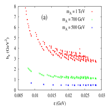
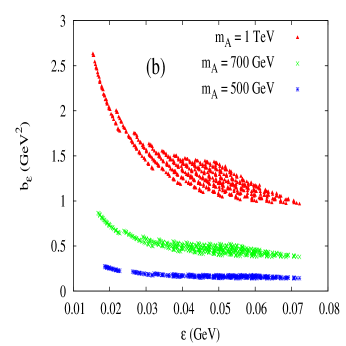
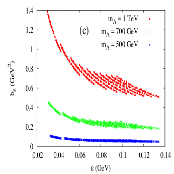
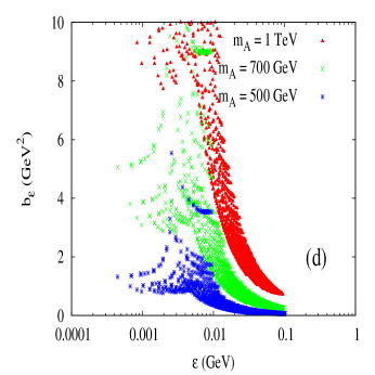
In Fig. 1(d) we have applied the constraint $R_{\gamma\gamma}\leq 1$, while in other plots of Fig. 1 the constraint $R_{\gamma\gamma}>1$ has been applied. In Fig. 1(a) $m_{L}$ has been kept to a very low value of 200 GeV, and in Figs. 1(b) and 1(c) $m_{L}=$ 300 and 400 GeV, respectively. As explained earlier, the allowed points in these plots are satisfied by the requirement $R_{\gamma\gamma}>1$. We have found that for $m_{L}=$ 150 GeV, the constraint $R_{\gamma\gamma}>1$ is not satisfied. From the plots of Fig. 1(a)$-$(c), we can notice that the most likely value of $\epsilon$ is $\mathrel{\raise 2.58334pt\hbox{$>$}\kern-7.7778pt\lower 2.79857pt\hbox{$\sim$}}$ 0.01 GeV. This value of $\epsilon$ is at least one order larger than its expected value from the neutrino masses, which is described at the end of Sec. 2.1. For $R_{\gamma\gamma}>1$, the lowest value of $\epsilon$ can be found in Fig. 1(a), which is $\approx$ 0.007 GeV, and at these points $M_{2}$ should be as low as 100 GeV. On the other hand, in future, if LHC has not found any excess in the Higgs to diphoton decay rate, then from Fig. 4(d) we can notice that we can satisfy the neutrino oscillation data for $\epsilon$ between about $10^{-4}$ to 0.1 GeV. In Fig. 4(d) we have fixed $m_{L}=$ 400 GeV. By decreasing $m_{L}$, the allowed space for $\epsilon$ and $b_{\epsilon}$ is slightly different from that of Fig. 4(d). Hence, from the measurement of Higgs to diphoton decay rate, if $R_{\gamma\gamma}>1$ then $\epsilon$ should be at least $\sim 10^{-2}$ GeV. Otherwise, if $R_{\gamma\gamma}\leq 1$ then $\epsilon$ can be as low as $\sim 10^{-4}$ GeV.

From the plots of Fig. 1(a)$-$(c), we can notice that when we increase $m_{L}$ by keeping $m_{A}$ fixed, the average value of $\epsilon$ is increasing. By increasing $m_{L}$, the lower limit on $\tan\beta$ and $\mu$ will increase in the case of $R_{\gamma\gamma}>1$, which we will describe below. As a result of this, the quantity $a_{0}$ of Eq. (8), which is inversely related to $\epsilon$, will decrease.

In Sec. 2.1, from the neutrino mass scale we have estimated that $b_{\epsilon}$ is $\sim$ 1 GeV². In the case of $R_{\gamma\gamma}>1$, from the plots of Fig. 1(a)$-$(c), we can notice that for $m_{A}\mathrel{\raise 2.58334pt\hbox{$>$}\kern-7.7778pt\lower 2.79857pt\hbox{$\sim$}}$ 700 GeV, $b_{\epsilon}$ can be in the range of 0.5 to 2 GeV². For $R_{\gamma\gamma}>1$, the lowest value of $b_{\epsilon}$ has been found to be about 0.05 GeV², which can be seen in Fig. 1(c). In Fig. 1(d) we have $R_{\gamma\gamma}\leq 1$, and the allowed value of $b_{\epsilon}$ can be around 1 GeV² by appropriately choosing the $m_{A}$. For instance, if we have to achieve $\epsilon\sim 10^{-3}$ GeV and $b_{\epsilon}\sim$ 1 GeV², then $m_{A}$ should be $\mathrel{\raise 2.58334pt\hbox{$<$}\kern-7.7778pt\lower 2.79857pt\hbox{$\sim$}}$ 500 GeV.

In Figs. 1(a)$-$(c), for a given value of $m_{L}$, $b_{\epsilon}$ is increasing with $m_{A}$. The reason for this is that $b_{\epsilon}$ is inversely related to $a_{1}$, and from Eq. (8) we can understand that $a_{1}$ decreases with $m_{A}$. Similarly, from Figs. 1(a)$-$(c), by keeping $m_{A}$ fixed, we can notice that the average value of $b_{\epsilon}$ is decreasing with $m_{L}$. We will shortly explain below that by increasing $m_{L}$ the lower limit on $\tan\beta$ and $\mu$ will increase in the case of $R_{\gamma\gamma}>1$. Hence, although the function $I_{4}$ of $a_{1}$ decreases with increasing $m_{L}$, the factor $\frac{1}{\cos^{2}\beta}$ in $a_{1}$ will compensate this decrease, and the net result is that $a_{1}$ increases with $m_{L}$.

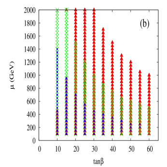
In Fig. 2 we have plotted allowed values of $\mu$ and $\tan\beta$. The points in Fig. 2(a) are allowed by the constraint $R_{\gamma\gamma}>1$, whereas the points in Fig. 2(b) satisfy $R_{\gamma\gamma}\leq 1$. In the plots of Fig. 2 there are no allowed points for $\tan\beta=5$. We have found that for such a low $\tan\beta$ the mass of light Higgs boson is below 123 GeV and hence do not satisfy the constraint (i).

Figure 2: Allowed values of $\mu$ and $\tan\beta$ for $m_{A}$ = 1 TeV. In plots (a) and (b) we have applied the constraints $R_{\gamma\gamma}>1$ and $R_{\gamma\gamma}\leq 1$, respectively. The red, green and blue points are for $m_{L}$ = 400, 300 and 200 GeV, respectively.

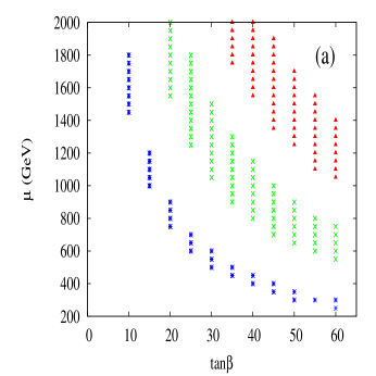
In Fig. 2(a), we can notice that by increasing the value of $m_{L}$, the lower limit on $\mu$ and $\tan\beta$ would increase. We may understand this from the fact that the stau masses should be as light as possible, and moreover, the mixing in the stau sector should be large in order to have $R_{\gamma\gamma}>1$ [17]. Hence, by increasing the soft mass $m_{L}$, the quantity $\mu\times\tan\beta$ should proportionately be increased in order to decrease the lightest stau mass and also to increase the mixing in the stau sector. From Fig. 2(a), we can notice that for a specific value of $\tan\beta$ the allowed value of $\mu$ lies in a certain range. We have seen that the lower and upper limits of this range are restricted by the constraints (ii) and (iii). For instance, for $m_{L}$ = 300 GeV and $\tan\beta$ = 30, the allowed range for $\mu$ is from 1050 to 1500 GeV. In this case, for $\mu<$ 1050 GeV we may not satisfy $R_{\gamma\gamma}>1$. On the other hand, for $\mu>$ 1500 GeV the lightest stau mass becomes less than 100 GeV. In Fig. 2(a) we have fixed $m_{A}$ = 1 TeV. By decreasing $m_{A}$, we have found that $\tan\beta$ is not restricted, however, for each $\tan\beta$ the corresponding lower limit on $\mu$ will increase. To illustrate this point, by considering the case of $m_{A}$ = 700 GeV, $m_{L}$ = 300 GeV and $\tan\beta$ = 30, the allowed range for $\mu$ has been found to be between 1150 to 1500 GeV. Hence, these results indicate that by decreasing $m_{A}$ the $R_{\gamma\gamma}$ value will decrease.

As stated before, in Fig. 2(b) we have applied the constraint $R_{\gamma\gamma}\leq 1$. In this plot we can see that $\mu$ can be as low as 100 GeV. Numerically, we have noticed that $R_{\gamma\gamma}$ increases with $\mu$ and hence after a certain large value of $\mu$, $R_{\gamma\gamma}\leq 1$ may not be satisfied. In the case of $m_{L}=$ 400 GeV, in Fig. 2(b), for $\tan\beta=$ 10 and 15, large values of $\mu$ are not allowed by the constraint (iv). In fact, allowed points in Fig. 2(b) indicate that $R_{\gamma\gamma}\leq 1$ can be satisfied for large $\tan\beta$ and relatively large $\mu$ values. For these large values of $\mu$ and $\tan\beta$, the calculated values of $\epsilon$ can be as high as 0.1 GeV, which can be seen in Fig. 1(d). For low $\tan\beta$ and moderate values of $\mu$, $\epsilon$ can be $\mathrel{\raise 2.58334pt\hbox{$<$}\kern-7.7778pt\lower 2.79857pt\hbox{$\sim$}}10^{-3}$ GeV.

In Fig. 3, we show the correlation between enhancement in the Higgs to diphoton decay rate ($R_{\gamma\gamma}$) and the bilinear parameter $\epsilon$.

Figure 3: Allowed values of $\epsilon$ versus $R_{\gamma\gamma}$. In the plots (a), (b) and (c), the value of $m_{L}$ = 200, 300 and 400 GeV, respectively. In these plots we have applied the constraint $R_{\gamma\gamma}>1$. In plot (d), $m_{L}=$ 400 GeV and the constraint $R_{\gamma\gamma}\leq 1$ has been applied. In each of these plots red, green and blue color points represent $m_{A}=$ 1000, 700 and 500 GeV, respectively.

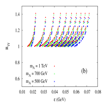
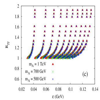
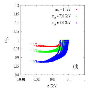
From Figs. 3(a)$-$(c), we can observe that for a low value of $m_{L}$ = 200 GeV, the maximum value for $R_{\gamma\gamma}$ is $\approx$ 1.1. As noted before, in the case of $R_{\gamma\gamma}>1$, the lowest value of $\epsilon$ is $\approx$ 0.007 GeV, which is found for $m_{L}=$ 200 GeV. For this lowest value of $\epsilon$ the $R_{\gamma\gamma}$ value is barely greater than 1.0. From Figs. 3(a)$-$(c), we can notice that the maximum value of $R_{\gamma\gamma}$ is increasing with $m_{L}$. We have stated before that by increasing $m_{L}$, the values of $\mu$ and $\tan\beta$ would increase. For large values of $\mu$ and $\tan\beta$, the coupling strengths of staus to the light Higgs boson would increase [17]. As a result of this, $R_{\gamma\gamma}$ is increasing with $m_{L}$. The maximum values of $R_{\gamma\gamma}$ in Figs. 3(b) and 3(c) are 1.41 and 1.92 respectively. We may increase $R_{\gamma\gamma}$ to more than 2.0 by increasing $m_{L}$ to 500 GeV. But in order to have large mixing and lower masses in the stau sector, we have to proportionately increase $\mu$ and $\tan\beta$. In this work we have scanned $\mu$ and $\tan\beta$ up to 2 TeV and 60, respectively, and have not considered cases of $m_{L}\geq$ 500 GeV. However, from the above mentioned arguments, for $R_{\gamma\gamma}>1$, we can speculate that by increasing $m_{L}$ to 500 GeV the value of $\epsilon$ would be around 0.1 GeV.

In Fig. 3(d), we have applied the constraint $R_{\gamma\gamma}\leq 1$. We can notice from this plot that for $\epsilon\sim 10^{-3}$ GeV, $R_{\gamma\gamma}$ is different for different values of $m_{A}$. From this perspective we can argue that, if $R_{\gamma\gamma}\leq 1$ is found to be true, then a precise measurement of $R_{\gamma\gamma}$ can be used to determine $\epsilon$ and $m_{A}$.

3.3 Smallness of $\epsilon$ and $b_{\epsilon}$

In this subsection, we try to motivate the smallness of $\epsilon$ and $b_{\epsilon}$ from a high scale physics. Essentially we will explore what the Higgs to diphoton decay rate can tell us about the high scale physics parameters. As it is noted in [14], by assuming supersymmetry breaking at an intermediate energy scale $\Lambda\sim 10^{11}$ GeV, we can explain the $\mu$-parameter, soft terms in scalar potential as well as $\epsilon$- and $b_{\epsilon}$- terms. Here we briefly describe important ingredients from Ref. [14]. By introducing SM gauge singlet superfields $\hat{S}$, $\hat{X}_{1}$ and $\hat{X}_{2}$, we may write the superpotential as

$$W=\Lambda^{2}\hat{S}+\frac{1}{M_{P}}\hat{X}_{1}^{3}\hat{X}_{2}+\frac{\hat{X}_{1}^{2}}{M_{P}}\hat{H}_{u}\hat{H}_{d}+\frac{\hat{X}_{2}^{3}}{M^{2}_{P}}\hat{L}\hat{H}_{u}+\cdots.$$ (31)

Here, $M_{P}=2.4\times 10^{18}$ GeV is the Planck scale. There can be ${\cal O}(1)$ couplings in the above terms, which we have neglected. In the above equation we have written only the necessary terms for our purpose, and these terms can be justified by introducing additional symmetries, say gauged $U(1)^{\prime}$. $\hat{S}$ must be singlet under this additional $U(1)^{\prime}$, but $\hat{X}_{1,2}$ can be charged under $U(1)^{\prime}$. The vevs of the scalar components of these SM gauge singlet superfields can be arranged as [14]: $\langle S\rangle\sim M_{P}$, $\langle X_{1,2}\rangle=\Lambda_{1,2}\sim\Lambda$. The first term of Eq. (31) breaks supersymmetry spontaneously by acquiring an auxiliary vev to $\hat{S}$ which is of the order of $\Lambda^{2}$. This axillary vev can generate soft terms in the scalar potential with mass parameters $m_{\rm soft}\sim\frac{\Lambda^{2}}{M_{P}}$. Here, the generation of soft terms in the scalar potential is based on the Polonyi mechanism [31]. The scalar vevs of $\hat{X}_{1,2}$ generate the $\mu$- and $\epsilon$-parameters which are $\mu\sim\frac{\Lambda_{1}^{2}}{M_{P}}$ and $\epsilon\sim\frac{\Lambda_{2}^{3}}{M_{P}^{2}}$. Here, we have followed the Kim-Nilles mechanism for the generation of $\mu$-term [32]. The auxiliary vevs of $\hat{X}_{1,2}$ can generate $b_{\mu}$ and $b_{\epsilon}$ which are $b_{\mu}\sim\frac{\Lambda_{1}^{3}\Lambda_{2}}{M_{P}^{2}}$ and $b_{\epsilon}\sim\frac{\Lambda_{1}^{3}\Lambda_{2}^{2}}{M_{P}^{3}}$.

In the previous paragraph, we have given motivation for the generation of $\epsilon$ and $b_{\epsilon}$ parameters as well as other supersymmetric parameters from a high scale physics. Now we have to fix the high scale physics parameters in order to fit the low energy data. Since we expect $m_{\rm soft}\sim\mu\sim$ TeV, for $\Lambda\sim\Lambda_{1}\sim 0.5\times 10^{11}$ GeV we can explain the TeV scale masses for supersymmetric fields. If we take $\Lambda_{2}\sim 10^{11}$ GeV we can get $\epsilon\sim 10^{-3}$ GeV. From Figs. 1 and 3, we can say that a value of $\epsilon\sim 10^{-3}$ GeV is consistent with $R_{\gamma\gamma}\leq 1$. In order to achieve $R_{\gamma\gamma}>1$, $\epsilon$ should be $\mathrel{\raise 2.58334pt\hbox{$>$}\kern-7.7778pt\lower 2.79857pt\hbox{$\sim$}}$ 0.01 GeV. Hence, by taking $\Lambda_{2}\sim 3.9\times 10^{11}$ GeV we can get $\epsilon\sim 10^{-2}$ GeV. So, if $R_{\gamma\gamma}>1$ then there is a little hierarchy between $\Lambda_{1}$ and $\Lambda_{2}$, otherwise, this hierarchy can be reduced.

In future, if LHC has found that $R_{\gamma\gamma}$ is significantly larger than 1.0, then from Figs. 3(a)$-$(c) we can say that $m_{L}$ should be larger than about 300 GeV. For $m_{L}$ between 300 to 400 GeV, from Figs. 1(b)and 1(c) we can have $b_{\epsilon}\sim$ 1 GeV², provided $m_{A}$ is $\mathrel{\raise 2.58334pt\hbox{$>$}\kern-7.7778pt\lower 2.79857pt\hbox{$\sim$}}$ 700 GeV. Now, for $\Lambda_{1}\sim 0.5\times 10^{11}$ GeV and $\Lambda_{2}\sim 3.9\times 10^{11}$ GeV, we can get $b_{\mu}\sim$ 8 TeV² and $b_{\epsilon}\sim$ 1 GeV². Hence, for the case of $R_{\gamma\gamma}>1$, we can motivate consistent supersymmetric mass spectrum and 0.1 eV scale for neutrino masses from a high scale physics by proposing two different intermediate scales. The hierarchy between these two scales should be at least 8.

If there is no enhancement in the Higgs to diphoton decay rate, from Fig. 1(d), we can notice that $\epsilon$ can be between $\sim 10^{-3}$ to 0.1 GeV. From the above discussion, to achieve $\epsilon\sim$ 0.1 GeV from high scale physics, there need to be little hierarchy between the intermediate scales $\Lambda_{1,2}$. This hierarchy can be minimal for $\epsilon\sim 10^{-3}$ GeV. For $\epsilon\sim 10^{-3}$ GeV, in Fig. 1(d), $b_{\epsilon}$ can be around 1 GeV² if $m_{A}\sim$ 500 GeV. For this set of values, from Fig. 3(d), we can notice that $R_{\gamma\gamma}$ is little less than 0.9. Hence, if we believe in the motivation of $\epsilon$ and $b_{\epsilon}$ from high scale physics, the high energy scales in this scenario depend on the value of $R_{\gamma\gamma}$. Moreover, in the above described analysis, we can also estimate $m_{L}$ and $m_{A}$ by knowing the $R_{\gamma\gamma}$. So the future runs at the LHC can give us clue about this scenario by precisely finding the $R_{\gamma\gamma}$.

We make short comments about measuring the parameters $\epsilon$ and $b_{\epsilon}$ in experiments. Since both these parameters indicate that R-parity is violated, a consequence of that is that the lightest supersymmetric particle (LSP) is unstable. Depending on the parameter space, either the lightest neutralino or the lightest charged slepton can be the LSP in this model [16]. The decay life time of LSP is determined by $\epsilon$ and $b_{\epsilon}$. Hence the signals of the decay of LSP in this model should give an indication about these bilinear parameters [16], from which we can verify the neutrino mass mechanism and also its correlation to the Higgs to diphoton decay rate.

4 Conclusions

Recently the LHC has discovered a Higgs-like particle whose mass is around 125 GeV. It has also been indicated that there is an enhancement in the Higgs to diphoton decay rate as compared to that in the SM. We have studied implications of these discoveries in the BRPVS model. This model is a minimal extension of the MSSM where the bilinear terms $\epsilon\hat{L}\hat{H}_{u}$ and $b_{\epsilon}\tilde{L}H_{u}$ are added to the superpotential and scalar potential of the model, respectively. The main objective of this model is to explain the smallness of neutrino masses, where the neutrino mass eigenvalues can be shown to be dependent on neutralino parameters, soft mass for charged sleptons ($m_{L}$) and CP-odd Higgs boson mass ($m_{A}$) [11, 12], apart from the bilinear parameters $\epsilon$ and $b_{\epsilon}$.

In our analysis, we have scanned over the neutralino parameters and varied $m_{L}$ and $m_{A}$ accordingly. We have also fixed the soft masses for third generation squarks, in order to have light Higgs boson mass to be around 125 GeV. We then have studied implications of enhancement in the Higgs to diphoton decay rate ($R_{\gamma\gamma}$) in the BRPVS model. Explicitly we have found that in order to be compatible with $R_{\gamma\gamma}>1$ and the neutrino oscillation data, the unknown bilinear parameter should be $\epsilon\mathrel{\raise 2.58334pt\hbox{$>$}\kern-7.7778pt\lower 2.79857pt\hbox{$\sim$}}10^{-2}$ GeV. We have also found that to achieve $R_{\gamma\gamma}$ between about 1.5 to 2.0, $m_{L}$ should be between 300 to 400 GeV, provided $\mu$ and $\tan\beta$ are scanned up to 2 TeV and 60 respectively. We have not obtained specific bounds on $m_{A}$. However, from the order of estimations we expect $b_{\epsilon}$ to be around 1 GeV² and to achieve this with the above mentioned $m_{L}$, $m_{A}$ can be in the range of 700 to 1000 GeV.

Since $R_{\gamma\gamma}>1$ is not yet confirmed by LHC, we have also analyzed the case of $R_{\gamma\gamma}\leq 1$. In this later case, we have found that $\epsilon$ can be between $\sim 10^{-3}$ to 0.1 GeV. The corresponding $b_{\epsilon}$ can be around 1 GeV² by appropriately choosing $m_{A}$ to be from 500 to 1000 GeV. Moreover, we have also found that $R_{\gamma\gamma}$ can be as low as 0.85.

From the above discussion, we can notice that $\epsilon$ and $b_{\epsilon}$ need to be very small in GeV units. We have motivated smallness of these two parameters from a high scale physics, and at the same time we have also explained the TeV scale masses for supersymmetric fields. We have found that to explain $\epsilon\sim 10^{-2}$ GeV and $b_{\epsilon}\sim$ 1 GeV² there need to be two different intermediate scales ($\sim 10^{11}$ GeV) with a hierarchy of factor of 8 between them.

References

- [1] G. Aad et al. [ATLAS Collaboration], Phys. Lett. B 716, 1 (2012) [arXiv:1207.7214 [hep-ex]]; S. Chatrchyan et al. [CMS Collaboration], Phys. Lett. B 716, 30 (2012) [arXiv:1207.7235 [hep-ex]].
- [2] F. Englert and R. Brout, Phys. Rev. Lett. 13, 321 (1964); P. W. Higgs, Phys. Lett. 12, 132 (1964); P. W. Higgs, Phys. Rev. Lett. 13, 508 (1964); G. S. Guralnik, C. R. Hagen and T. W. B. Kibble, Phys. Rev. Lett. 13, 585 (1964); P. W. Higgs, Phys. Rev. 145, 1156 (1966); T. W. B. Kibble, Phys. Rev. 155, 1554 (1967).
- [3] Please see the talk by F. Hubaut in the conference Rencontres de Moriond (EW Interactions and Unified Theories), https://indico.in2p3.fr/conferenceDisplay.py?confId=7411
- [4] Please see the talk by C. Ochando in the conference Rencontres de Moriond (QCD and High Energy Interactions), http://moriond.in2p3.fr/QCD/2013/qcd.html
- [5] H. P. Nilles, Phys. Rept. 110, 1 (1984); H. E. Haber and G. L. Kane, Phys. Rept. 117, 75 (1985); S. P. Martin, arXiv:hep-ph/9709356; M. Drees, R. Godbole and P. Roy, Theory and Phenomenology of Sparticles, (World Scientific, 2004); P. Binetruy, Supersymmetry (Oxford University Press, 2006); H. Baer and X. Tata, Weak Scale Supersymmetry: From Superfields to Scattering Events, (Cambridge University Press, 2006).
- [6] Y. Fukuda et al. [Kamiokande Collaboration], Phys. Rev. Lett. 77, 1683 (1996); W. Hampel et al. [GALLEX Collaboration], Phys. Lett. B 447, 127 (1999); J. N. Abdurashitov et al. [SAGE Collaboration], Phys. Rev. C 60, 055801 (1999) [astro-ph/9907113]; Q. R. Ahmad et al. [SNO Collaboration], Phys. Rev. Lett. 87, 071301 (2001) [nucl-ex/0106015]; K. Eguchi et al. [KamLAND Collaboration], Phys. Rev. Lett. 90, 021802 (2003) [hep-ex/0212021]; J. Hosaka et al. [Super-Kamiokande Collaboration], Phys. Rev. D 73, 112001 (2006) [hep-ex/0508053]; Y. Fukuda et al. [Super-Kamiokande Collaboration], Phys. Rev. Lett. 81, 1562 (1998) [hep-ex/9807003]; M. Ambrosio et al. [MACRO Collaboration], Phys. Lett. B 434, 451 (1998) [hep-ex/9807005].
- [7] E. Komatsu et al. [WMAP Collaboration], Astrophys. J. Suppl. 180, 330 (2009) [arXiv:0803.0547 [astro-ph]]; J. Dunkley et al. [WMAP Collaboration], Astrophys. J. Suppl. 180, 306 (2009) [arXiv:0803.0586 [astro-ph]].
- [8] C. .Kraus, B. Bornschein, L. Bornschein, J. Bonn, B. Flatt, A. Kovalik, B. Ostrick and E. W. Otten et al., Eur. Phys. J. C 40, 447 (2005) [hep-ex/0412056].
- [9] M. Hirsch and J. W. F. Valle, New J. Phys. 6, 76 (2004) [hep-ph/0405015].
- [10] M. Hirsch, M. A. Diaz, W. Porod, J. C. Romao and J. W. F. Valle, Phys. Rev. D 62, 113008 (2000) [Erratum-ibid. D 65, 119901 (2002)] [hep-ph/0004115]; M. A. Diaz, M. Hirsch, W. Porod, J. C. Romao and J. W. F. Valle, Phys. Rev. D 68, 013009 (2003) [Erratum-ibid. D 71, 059904 (2005)] [hep-ph/0302021].
- [11] S. Davidson and M. Losada, JHEP 0005, 021 (2000) [hep-ph/0005080], Phys. Rev. D 65, 075025 (2002) [hep-ph/0010325].
- [12] Y. Grossman and S. Rakshit, Phys. Rev. D 69, 093002 (2004) [hep-ph/0311310].
- [13] A. Masiero and J. W. F. Valle, Phys. Lett. B 251, 273 (1990); J. C. Romao, C. A. Santos and J. W. F. Valle, Phys. Lett. B 288, 311 (1992); J. C. Romao, A. Ioannisian and J. W. F. Valle, Phys. Rev. D 55, 427 (1997) [hep-ph/9607401].
- [14] R. S. Hundi, S. Pakvasa and X. Tata, Phys. Rev. D 79, 095011 (2009) [arXiv:0903.1631 [hep-ph]].
- [15] A. S. Joshipura and M. Nowakowski, Phys. Rev. D 51, 2421 (1995) [hep-ph/9408224]; R. Hempfling, Nucl. Phys. B 478, 3 (1996) [hep-ph/9511288]; S. Roy and B. Mukhopadhyaya, Phys. Rev. D 55, 7020 (1997) [hep-ph/9612447]; B. Mukhopadhyaya, S. Roy and F. Vissani, Phys. Lett. B 443, 191 (1998) [hep-ph/9808265]; S. Y. Choi, E. J. Chun, S. K. Kang and J. S. Lee, Phys. Rev. D 60, 075002 (1999) [hep-ph/9903465]; A. S. Joshipura, R. D. Vaidya and S. K. Vempati, Phys. Rev. D 62, 093020 (2000) [hep-ph/0006138]; A. S. Joshipura, R. D. Vaidya and S. K. Vempati, Nucl. Phys. B 639, 290 (2002) [hep-ph/0203182]; F. de Campos, O. J. P. Eboli, M. B. Magro, W. Porod, D. Restrepo, M. Hirsch and J. W. F. Valle, JHEP 0805, 048 (2008) [arXiv:0712.2156 [hep-ph]]; D. Restrepo, M. Taoso, J. W. F. Valle and O. Zapata, Phys. Rev. D 85, 023523 (2012) [arXiv:1109.0512 [hep-ph]]; F. Bazzocchi, S. Morisi, E. Peinado, J. W. F. Valle and A. Vicente, JHEP 1301, 033 (2013) [arXiv:1202.1529 [hep-ph]]; E. Peinado and A. Vicente, Phys. Rev. D 86, 093024 (2012) [arXiv:1207.6641 [hep-ph]]; A. Arhrib, Y. Cheng and O. C. W. Kong, arXiv:1210.8241 [hep-ph].
- [16] W. Porod, M. Hirsch, J. Romao and J. W. F. Valle, Phys. Rev. D 63, 115004 (2001) [hep-ph/0011248]; M. Hirsch, W. Porod, J. C. Romao and J. W. F. Valle, Phys. Rev. D 66, 095006 (2002) [hep-ph/0207334]; A. Bartl, M. Hirsch, T. Kernreiter, W. Porod and J. W. F. Valle, JHEP 0311, 005 (2003) [hep-ph/0306071]; F. de Campos, O. J. P. Eboli, M. B. Magro, W. Porod, D. Restrepo, S. P. Das, M. Hirsch and J. W. F. Valle, Phys. Rev. D 86, 075001 (2012) [arXiv:1206.3605 [hep-ph]]; D. Aristizabal Sierra, D. Restrepo and S. Spinner, arXiv:1212.3310 [hep-ph].
- [17] M. Carena, S. Gori, N. R. Shah and C. E. M. Wagner, JHEP 1203, 014 (2012) [arXiv:1112.3336 [hep-ph]]; M. Carena, S. Gori, N. R. Shah, C. E. M. Wagner and L. -T. Wang, JHEP 1207, 175 (2012) [arXiv:1205.5842 [hep-ph]].
- [18] J. Cao, Z. Heng, T. Liu and J. M. Yang, Phys. Lett. B 703, 462 (2011) [arXiv:1103.0631 [hep-ph]]; J. -J. Cao, Z. -X. Heng, J. M. Yang, Y. -M. Zhang and J. -Y. Zhu, JHEP 1203, 086 (2012) [arXiv:1202.5821 [hep-ph]]; J. Cao, Z. Heng, J. M. Yang and J. Zhu, JHEP 1210, 079 (2012) [arXiv:1207.3698 [hep-ph]].
- [19] A. Arbey, M. Battaglia, A. Djouadi and F. Mahmoudi, JHEP 1209, 107 (2012) [arXiv:1207.1348 [hep-ph]].
- [20] U. Ellwanger, JHEP 1203, 044 (2012) [arXiv:1112.3548 [hep-ph]]; K. Schmidt-Hoberg and F. Staub, JHEP 1210, 195 (2012) [arXiv:1208.1683 [hep-ph]].
- [21] A. Djouadi, Phys. Rept. 459, 1 (2008) [hep-ph/0503173].
- [22] T. Kitahara, JHEP 1211, 021 (2012) [arXiv:1208.4792 [hep-ph]]; T. Kitahara, T. Yoshinaga and , arXiv:1303.0461 [hep-ph].
- [23] J. Beringer et al. (Particle Data Group), Phys. Rev. D 86, 010001 (2012).
- [24] Y. Abe et al. [DOUBLE-CHOOZ Collaboration], Phys. Rev. Lett. 108, 131801 (2012) [arXiv:1112.6353 [hep-ex]]; F. P. An et al. [DAYA-BAY Collaboration], Phys. Rev. Lett. 108, 171803 (2012) [arXiv:1203.1669 [hep-ex]]; J. K. Ahn et al. [RENO Collaboration], Phys. Rev. Lett. 108, 191802 (2012) [arXiv:1204.0626 [hep-ex]].
- [25] D. V. Forero, M. Tortola and J. W. F. Valle, arXiv:1205.4018 [hep-ph].
- [26] P. F. Harrison, D. H. Perkins and W. G. Scott, Phys. Lett. B 530, 167 (2002) [hep-ph/0202074].
- [27] R. S. Hundi, Phys. Rev. D 83, 115019 (2011) [arXiv:1101.2810 [hep-ph]].
- [28] A. Djouadi, J. Kalinowski and M. Spira, Comput. Phys. Commun. 108, 56 (1998) [hep-ph/9704448].
- [29] For a review on the muon , see, Z. Zhang, arXiv:0801.4905 [hep-ph]; F. Jegerlehner and A. Nyffeler, Phys. Rept. 477, 1 (2009) [arXiv:0902.3360 [hep-ph]].
- [30] T. Moroi, Phys. Rev. D 53, 6565 (1996) [Erratum-ibid. D 56, 4424 (1997)] [hep-ph/9512396]; S. P. Martin and J. D. Wells, Phys. Rev. D 64, 035003 (2001) [hep-ph/0103067].
- [31] J. Polonyi, Hungary Central Research Institute Report No. KFKI-77-93, 1977 (unpublished).
- [32] J. E. Kim and H. P. Nilles, Phys. Lett. B 138, 150 (1984).