Two-channel Bose-Hubbard model of atoms at a Feshbach resonance

Abstract

Based on the analytic model of Feshbach resonances in harmonic traps described in Phys. Rev. A 83, 030701 (2011) a Bose-Hubbard model is introduced that provides an accurate description of two atoms in an optical lattice at a Feshbach resonance with only a small number of Bloch bands. The approach circumvents the problem that the eigenenergies in the presence of a delta-like coupling do not converge to the correct energies, if an uncorrelated basis is used. The predictions of the Bose-Hubbard model are compared to non-perturbative calculations for both the stationary states and the time-dependent wavefunction during an acceleration of the lattice potential. For this purpose, a square-well interaction potential is introduced, which allows for a realistic description of Feshbach resonances within non-perturbative single-channel calculations.

I Introduction

Since the creation of the first Bose-Einstein condensates Anderson et al. (1995); Davis et al. (1995), ultracold atoms have proven to be a versatile tool for many applications like precision measurement, quantum simulation, and quantum information processing. Two of the main techniques that made these achievements possible are the creation of various trapping potentials, like optical lattices (OLs) or wave guides and the precise control of the interatomic interaction by means of Feshbach resonances (FRs) Bloch et al. (2008); Chin et al. (2010).

An important tool for describing ultracold atoms in OLs is the Bose-Hubbard (BH) model. The model uses in its basic form a basis of single-particle Wannier states from the first Bloch band to formulate the many-body Hamiltonian. While for weak interactions the model is very accurate, it usually breaks down for larger scattering lengths. A way to extend its applicability at a broad FR is to introduce effective BH parameters especially for the onsite interaction strength $U$. These parameters can be obtained by using a corrected harmonic approximation of the lattice sites Schneider et al. (2009) or by full numerical calculations Büchler (2010, 2012).

The usual BH model allows via the onsite-interaction strength $U$ either for repulsively interacting atoms ($U>0$) or attractively interacting atoms ($U<0$). At a narrow FR, however, a relatively narrow avoided crossing with the resonant bound state leads to the appearance of both repulsively and attractively interacting states Schneider et al. (2011); Sanders et al. (2011). In this situation the resonant bound state must be explicitly included into the BH model. Several different kinds of these extended models have been introduced and debated Dickerscheid et al. (2005); Diener and Ho (2006); Dickerscheid et al. (2006); Sanders et al. (2011) and applied to map out the phase diagramm Dickerscheid et al. (2005); Carr and Holland (2005); Rousseau and Denteneer (2009) or to investigate lattice solitons Krutitsky and Skryabin (2006).

The above investigations consider the extended Hubbard model within a single-band approximation that is only applicable in the rare situation that the coupling energy to the resonant bound state is small compared to the band gap. In order to generalize the applicability one can introduce the notion of dressed molecules with effective bound-state energies and coupling strengths obtained from more elaborate calculations Wall and Carr (2012).

A convenient approach to generalize Hubbard models to describe broader FRs or systems with a large scattering length is to simply include more Bloch bands. For example, L.-M. Duan has derived an effective single-band Hubbard model for the case of interacting fermions at a broad FR starting from a multi-band Hubbard model in the Wannier basis and a zero-range coupling between atoms and molecules Duan (2005). However, as will be discussed in this work, severe numerical problems arise for the description of a system with a zero-range coupling, e.g., by expanding the solution in products of single-particle basis functions. Especially for large scattering lengths all of these basis functions behave completely differently for $r\rightarrow 0$ compared with the correct solution. This poses a problem especially for positive scattering lengths where the open channel supports a bound state. In fact, the obtained energies are lower than the correct ones so that an increase of the basis leads to an even larger disagreement. A similar problem also appears when replacing the interaction potential by the delta-like Fermi-Huang pseudo-potential Esry and Greene (1999). Also within analytical treatments of FRs in harmonic traps that use non-interacting basis states the eigenenergies do not converge Dickerscheid et al. (2005); Jachymski et al. (2013). In this case, after an infinite summation, the diverging terms can be absorbed by introducing a renormalized bound-state energy. In many numerical approaches the problem is circumvented by replacing the delta-like potential by a regularized short range potential Büchler (2010, 2012); Brouzos and Schmelcher (2012). In order to resolve the potential usually a large basis is necessary. For example, for an interaction with the range $d/N$ where $d$ is the lattice spacing more than $N$ Bloch bands have to be included to converge the energies Büchler (2010, 2012). Since for two atoms in a one dimensional lattice the number of basis functions scales quadratically with the number of Bloch bands and the number of sites the solution can quickly become numerically very demanding. Based on this corrected numerical approach, M.L. Wall and L.D. Carr were able to calculated the effective parameters of a Fermi Hubbard model that takes the coupling to a bosonic molecule explicitly into account Wall and Carr (2012).

In this work we introduce an extended BH model that avoids the numerical problems in the presence of a delta-like coupling without the need of regularization and inclusion of many Bloch bands. The model is derived from first principles on the basis of the analytic microscopic theory of FRs in a harmonic trap Schneider et al. (2011). This allows for defining dressed bound-state energies and couplings that correct for the problems due to the deficiency of the basis states.

Given the number of different proposals to describe FRs within a BH model one has to compare the predictions of the introduced BH model with non-perturbative calculations. In the standard description of FRs this requires to solve a two-channel problem of two interacting atoms in an optical lattice coupled at short distance to a molecular bound state. This problem is numerically very demanding. However, we show that one can largely simplify the problem by introducing a square-well interaction potential that realistically mimics the behavior at a FR. Using this single-channel interaction potential we apply an approach introduced in Grishkevich et al. (2011); Schneider et al. (2012) in order to obtain the correct energies and wave functions of two atoms in a small OL at a FR. The correct stationary and dynamic behavior of two atoms in a double-well potential is compared with the results of the introduced BH model. It is shown that with only a small number of Bloch bands included the BH model is able to accurately describe FRs of small and medium width with coupling energies up to the depth of the OL.

The work is organized as follows. First the analytic model of a FR in a harmonic introduced in Schneider et al. (2011) is briefly recapitulated. This sets the basis for the derivation of a general BH model of interacting atoms at a FR in Sec. III. The model is compared to the exact analytical solution in a harmonic trap in Sec. IV, revealing that the BH model does not converge toward the correct eigenenergies. To circumvent this problem dressed molecular states and a dressed coupling strength of the BH model are introduced in Sec. V on the basis of the analytically known eigenenergies in the harmonic trap. In Sec. VI the square-well interaction potential is discussed, which allows for finding within a non-perturbative approach both the stationary and the time-dependent wavefunctions of two atoms in a small OL at a FR perturbed by a time-dependent acceleration of the lattice. Finally, in Sec. VII the dressed and undressed BH model is compared to the non-perturbative calculations. We conclude in Sec. VIII.

II Feshbach resonance in a harmonic trap

Neutral atoms usually only interact at small distances $r$ on the order of $r_{\rm int}\sim 100\,$a.u. which is much smaller than typical length scales of the trapping potentials on the order of some $r_{\rm trap}\sim 10\,000\,$a.u. The collision energy in the ultracold regime is so small that partial waves with angular momentum $l>0$ are reflected by the centrifugal barrier. Therefore $s$-wave ($l=0$) scattering is largely dominant. For $r_{\rm int}\ll r\ll r_{\rm trap}$ the interaction leads to a phase shift $\varphi$ of the scattering wave function $\propto\sin(kr+\varphi)$ which is associated with the $s$-wave scattering length $a(k)=-\tan(\varphi)/k$.

If two atoms collide, the spin states of the scattering atoms are coupled at small distances $r\leq r_{\rm int}$ to other spin states in closed channels whose relative energy can be influenced by applying an external magnetic field $B$. The subspace of closed-channel spin states can support many bound states. For certain magnetic field strengths $B$ the energy of such a bound state $E_{b}(B)$ can be brought into resonance with the collision energy $E$ of the atoms, leading to a FR (see Fig. 1).

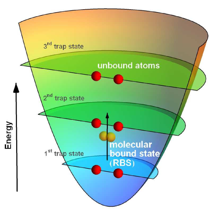
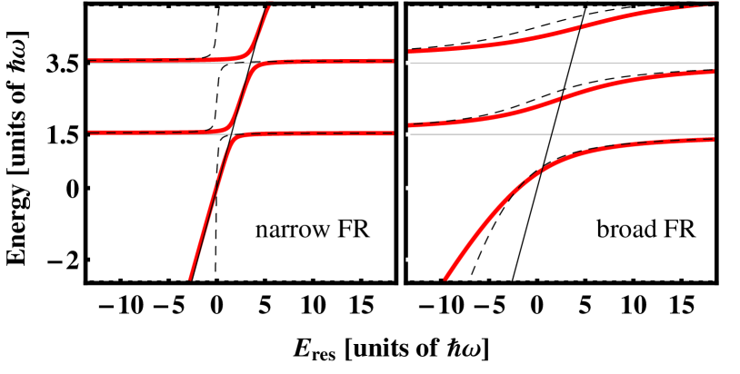
Figure 1: (Color online). Mechanism of broad and narrow FRs in the exemplary case of two atoms in isotropic harmonic confinement with frequency $\omega$. Top: Sketch of the relative-motion unbound trap states and the resonant molecular bound state (RBS) whose energy can be manipulated by an external magnetic field. Bottom: Relative-motion energy spectrum [solutions of Eq. (12)] using the energy-dependent scattering length $a(E,E_{\rm res})$ (thick red lines) and the energy-independent scattering length $a(0,E_{\rm res})$ (black dashed line) as a function of the resonance energy $E_{\rm res}=E_{b}+\delta E$ (black solid line). At a narrow FR (left: $a_{\rm bg}=0.04a_{\rm ho},\Delta E=1\hbar\omega$) the RBS couples only to the trap state that is in resonance, which leads to narrow avoided crossings. At a broad FR (right: $a_{\rm bg}=0.04a_{\rm ho},\Delta E=40\hbar\omega$) the RBS couples to many trap states and the energy spectrum changes globally with $E_{\rm res}$. In contrast to the narrow FR the eigenenergies for an energy-dependent and energy-independent scattering length agree reasonably for broad resonances.

In Schneider et al. (2011) an analytic model for a FR in isotropic and anisotropic harmonic traps was developed. Its starting point is the relative-motion (REL) Hamiltonian for radial momentum $l=0$ of two atoms in a spherical harmonic confinement with frequency $\omega$. The Hamiltonian for the radial wave function $\left|\Phi(r)\right>=\sqrt{4\pi}r\left|\Psi(r)\right>$, where $\left|\Psi(r\,)\right>$ is the REL wave function, is given as

$$\hat{\rm H}=-\frac{\hbar^{2}}{2\mu}\frac{d^{2}}{dr^{2}}+\frac{1}{2}\mu\omega^{2}r^{2}+\hat{\rm V}_{\rm ZH}+\hat{\rm V}_{\rm int}(r).$$ (1)

Here, $\mu$ is the reduced mass, $\hat{\rm V}_{\rm ZH}$ is the Zeeman and hyperfine energy of the atoms, and $\hat{\rm V}_{\rm int}(r)$ the electron-spin dependent interaction potential.

One assumes that the REL energy of the atoms is small enough so that only one spin configuration (the open channel) supports unbound states. All other spin configurations are closed, i.e. their wave function vanishes for large interatomic distances.

The analytic model is based on the two-channel description of an FR where one channel represents the unbound atoms and the other channel the subspace of closed channels. By introducing projectors $\hat{\rm P}$ and $\hat{\rm Q}$ onto the subspace of open and closed channels, respectively, one arrives at the coupled equations

$$(\hat{\rm H}_{P}-E)\left|\Phi_{P}\right>+\hat{\rm W}\left|\Phi_{Q}\right> = 0\,,$$ (2)

$$(\hat{\rm H}_{Q}-E)\left|\Phi_{Q}\right>+\hat{\rm W}^{\dagger}\left|\Phi_{P}\right> = 0\,,$$ (3)

with $\hat{\rm H}_{P}=\hat{\rm P}\hat{\rm H}\hat{\rm P}$, $\hat{\rm H}_{Q}=\hat{\rm Q}\hat{\rm H}\hat{\rm Q}$, $\hat{\rm W}=\hat{\rm P}\hat{\rm H}\hat{\rm Q}$, $\left|\Phi_{P}\right>=\hat{\rm P}\left|\Phi\right>$, $\left|\Phi_{Q}\right>=\hat{\rm Q}\left|\Phi\right>$, and $E$ the energy above the threshold of the open-channel interaction potential. Since the eigenenergies in the closed channel subspace are usually largely separated on the energy scale $\hbar\omega$ of the trap, one assumes that close to the FR $\left|\Phi_{Q}\right>$ is simply a multiple $A$ of a single bound eigenstate $\left|\phi_{b}\right>$ with eigenenergy $E_{b}$. We call this closed-channel state “resonant bound state” (RBS). To first order, the energy $E_{b}$ may be expanded linearly in the magnetic field $B$, i.e. $E_{b}(B)=\sigma(B-B_{0})$, where $\sigma$ is the relative magnetic moment that is known for many FRs Chin et al. (2010).

Introducing the normalized solution $\left|\phi_{E}\right>$ of the open channel with $\left|\Phi_{P}\right>=C\left|\phi_{E}\right>$ and a background eigenstate $\left|\phi_{\rm bg}\right>$ of $\hat{\rm H}_{P}$ with eigenenergy $E_{\rm bg}$ which is occupied for infinite detuning $|E-E_{b}|\rightarrow\infty$ one obtains the eigenenergy equation Schneider and Saenz (2009)

$$(E-E_{b})(E-E_{\rm bg})=\frac{\left<\phi_{\rm bg}\right|\hat{\rm W}\left|\phi_{b}\right>\left<\phi_{b}\right|\hat{\rm W}^{\dagger}\left|\phi_{E}\right>}{\left<\phi_{\rm bg}\vphantom{\phi_{E}}\right|\left.\phi_{E}\vphantom{\phi_{\rm bg}}\right>}\,.$$ (4)

In order to find simplified expressions for $\left<\phi_{\rm bg}\right|\hat{\rm W}\left|\phi_{b}\right>$, $\left<\phi_{b}\right|\hat{\rm W}^{\dagger}\left|\phi_{E}\right>$, and $\left<\phi_{\rm bg}\vphantom{\phi_{E}}\right|\left.\phi_{E}\vphantom{\phi_{\rm bg}}\right>$ one assumes that the interaction is only relevant in some small range $r<r_{\rm int}$ much smaller than the extension of the trap $r_{\rm trap}$. The extension of the harmonic trap is specified by the harmonic trap length $a_{\rm ho}=\sqrt{\hbar/(\mu\omega)}$. Denoting the long-range behavior of $\phi_{E}(r)$ by $\tilde{\phi}_{E}(r)$ one finds

$$\tilde{\phi}_{E}(r)\equiv\lim_{r\rightarrow\infty}\phi_{E}(r)=A_{\nu}D_{\nu}(\rho),$$ (5)

where $D_{\nu}(\rho)$ is the parabolic cylinder function, $\rho=\sqrt{2}r/a_{\rm ho}$, $\nu=E/(\hbar\omega)-1/2$, and $A_{\nu}$ is a normalization constant.

For $r\ll a_{\rm ho}$ the linear approximation of $D_{\nu}(\rho)$ yields Abramowitz and Stegun (1965)

$$\begin{split}\tilde{\phi}_{E}(r)&=\tilde{\phi}_{E}(0)+r\tilde{\phi}^{\prime}_{E}(0)+\mathcal{O}(r^{2})\\ &=\tilde{\phi}_{E}(0)\left(1-\frac{r}{a_{\rm ho}f(E)}\right)+\mathcal{O}(r^{2})\end{split}$$ (6)

with

$$f(E)=\frac{\Gamma\left(\frac{1}{4}-\frac{E}{2\hbar\omega}\right)}{2\Gamma\left(\frac{3}{4}-\frac{E}{2\hbar\omega}\right)},$$ (7)

where $\Gamma(x)$ is the Gamma function. In the range $r_{\rm int}\ll r\ll a_{\rm ho}$ the radial wavefunction with scattering length $a$ has the form $\phi_{E}(r)\propto 1-r/a$. Hence, one can directly determine the scattering length of the radial wave function with energy $E$ from Eq. (6). This yields

$$a=-\frac{\tilde{\phi}_{E}(0)}{\tilde{\phi}^{\prime}_{E}(0)}=a_{\rm ho}f(E)\,,$$ (8)

which is equivalent to the result in Busch et al. (1998).

In the spirit of a Taylor expansion we parametrize $\left<\phi_{E}\right|\hat{\rm W}\left|\phi_{b}\right>$ by a linear combination

$$\begin{split}\left<\phi_{b}\right|\hat{\rm W}^{\dagger}\left|\phi_{E}\right>&=\gamma\,\tilde{\phi}_{E}(0)+\beta\,\tilde{\phi}_{E}^{\prime}(0)\\ &=\gamma\,\tilde{\phi}_{E}(0)\left(1+\beta\,\frac{\tilde{\phi}_{E}^{\prime}(0)}{\gamma\,\tilde{\phi}_{E}(0)}\right)\\ &=\gamma\,\tilde{\phi}_{E}(0)\left(1-\frac{a^{*}}{a}\right)\end{split}$$ (9)

with $a^{*}=\beta/\gamma$. Be $\psi_{b}(r)=\phi_{b}(r)/(\sqrt{4\pi}r)$ the wave function describing the RBS then the expansion (9) can be interpreted as approximating the coupling to the bound state by $W(r)\psi_{b}(r)\approx\sqrt{4\pi}\gamma(r-a^{*})\delta(\vec{r}\,)$. For the long-range behavior of the wavefunction $\psi_{E}(r)$, i.e. $\lim_{r\rightarrow\infty}\psi_{E}(r)=\tilde{\psi}_{E}(r)=\tilde{\phi}_{E}(r)/(\sqrt{4\pi}r)$ one finds

$$\begin{split}\gamma\,\tilde{\phi}_{E}(0)&+\beta\,\tilde{\phi}_{E}^{\prime}(0)\\ &=\int dr\tilde{\phi}_{E}(r)\left[\gamma\delta(r)+\beta\delta^{\prime}(r)\right]\\ &=\int dr\sqrt{4\pi}\tilde{\psi}_{E}(r)\left[\gamma r-\beta\right]\delta(r)\\ &=\int r^{2}dr\,d\Omega\,\tilde{\psi}_{E}(r)\sqrt{4\pi}\gamma\left[r-a^{*}\right]\delta(\vec{r}).\end{split}$$ (10)

Here one uses $r\delta^{\prime}(r)=-\delta(r)$ and $\delta(r)=4\pi r^{2}\delta(\vec{r})$. Although only two parameters are used, the parametrization of the coupling is already quite general since higher order couplings like those proportional to $r^{2}\delta(\vec{r})$ automatically vanish. Within the approximation of a constant RBS $\gamma$ and $a^{*}$ must be constant. In reality, however, $\left<\phi_{b}\right|\hat{\rm W}^{\dagger}\left|\phi_{E}\right>$ depends on the nodal structure of the RBS and the open channel that are both not constant for a varying magnetic field. A comparison with complete coupled-channel calculations shows that it suffices to introduce a background coupling strength $\gamma_{\rm bg}$ for the parametrization of $\left<\phi_{\rm bg}\right|\hat{\rm W}\left|\phi_{b}\right>$ to account for slight variations of the nodal structure Schneider et al. (2011). Since the difference between $\gamma$ and $\gamma_{\rm bg}$ is only relevant for the RBS admixture but not for the eigenenergies of the system, we can ignore it for our purposes. Following the reasoning given in Schneider et al. (2011), the short-range approximation (9) then gives

$$E-E_{b}=\frac{2\gamma^{2}}{a_{\rm ho}\hbar\omega}\frac{\left(f(E)-\frac{a^{*}}{a_{\rm ho}}\right)\left(f(E_{\rm bg})-\frac{a^{*}}{a_{\rm ho}}\right)}{f(E)-f(E_{\rm bg})}\,.$$ (11)

The solutions of this equation determine the eigenenergies. One can rewrite this equation in the form of a matching condition: The scattering length $a(E,E_{b})$ due to the short-range coupling to the RBS must be equal to the product $a_{\rm ho}f(E)$ that is equal to the scattering length of the long-range wavefunction $\tilde{\phi}_{E}(r)$. This yields

$$a_{\rm ho}f(E)=a(E,E_{\rm res})=a_{\rm bg}(E)\left(1-\frac{\Delta E}{E_{\rm res}-E}\right)\,.$$ (12)

The right-hand side of the Eq. (12) describes the energy dependence of the scattering length with background scattering length $a_{\rm bg}$ and resonance width

$$\Delta E=\frac{2\gamma^{2}\mu a_{\rm bg}}{\hbar^{2}}\left(1-\frac{a^{*}}{a_{\rm bg}}\right)^{2}\,.$$ (13)

The resonance energy $E_{\rm res}=E_{b}+\delta E$ is shifted from the bound state energy $E_{b}$ by the resonance detuning

$$\delta E=\frac{a_{\rm bg}\Delta E}{a_{\rm bg}-a^{*}}\,.$$ (14)

In the limit $E\rightarrow 0$ the ratio of the resonance detuning and the resonance width is given as $\delta E/\Delta E=a_{0}/(a_{0}-a^{*})$, where $a_{0}=\lim_{E\rightarrow 0}a_{\rm bg}$ is the zero-energy background scattering length. Comparing this with the same ratio derived on the basis of a multi-channel quantum defect theory for $E\rightarrow 0$ Góral et al. (2004) allows for removing one free parameter $a^{*}$. One finds

$$a^{*}=\overline{a}\left(1+\frac{\overline{a}}{\overline{a}-a_{0}}\right)\,,$$ (15)

where the mean scattering length $\overline{a}$ is determined by the $C_{6}$ coefficient of the van der Waals interaction Gribakin and Flambaum (1993). Using Eqs. (13) and (15), the remaining parameter $\gamma$ can be directly related to the resonance width $\Delta E$.

The function $a_{\rm ho}f(E)$ which describes the scattering length of the wave function $\tilde{\phi}_{E}(r)$ is also known for anisotropic traps with $\omega_{y}=\omega_{z}=\eta\omega_{x}$. In this case the scattering length is given as $a=-\sqrt{\pi}d/\mathcal{F}(u,\eta)$ (with $d,u=u(E),$ and $\mathcal{F}$ defined in Idziaszek and Calarco (2006)) such that the eigenenergy relation

$$-\frac{\sqrt{\pi}d}{\mathcal{F}(u,\eta)}=a_{\rm bg}(E)\left(1-\frac{\Delta E}{E_{\rm res}-E}\right)\,$$ (16)

holds.

One generally distinguishes between narrow and broad FRs Chin et al. (2010). In the case of a broad FR the coupling strength to the bound state is relatively large such that it is admixed to unbound states in a large energy domain. If, as usual, the background scattering length $a_{\rm bg}$ is small compared to the trap length $a_{\rm ho}$, the ratio of the RBS admixture $|A|^{2}$ to the open-channel admixture $|C|^{2}$ for states above the first trap state is on the order of $a_{\rm ho}\hbar\omega/(a_{\rm bg}\Delta E)$ such that the RBS admixture can be neglected if $a_{\rm bg}\Delta E\gg a_{\rm ho}\hbar\omega$ Schneider et al. (2011). Furthermore, also the energy dependence of the scattering length becomes negligible if $a_{\rm bg}\Delta E\gg a_{\rm ho}\hbar\omega$ (see Fig. 1). Therefore, all details of the atomic interaction apart from the value of scattering length for $E\rightarrow 0$ are irrelevant. This situation is called universal. On the other hand, for narrow FRs the bound state couples only to a narrow energy range of scattering states or respectively to that unbound trap state which is in resonance. As shown in Fig. 1 in a harmonic trap this leads to narrow avoided crossings in the energy spectrum with an energy splitting on the order of $\sqrt{a_{\rm bg}\Delta E/(a_{\rm ho}\hbar\omega)}\hbar\omega$ Schneider et al. (2011). At the resonance the bound state is strongly admixed and the energy dependence of the scattering length cannot be neglected.

III Feshbach resonance in an optical lattice

In order to avoid unnecessary complexity, in the following an OL is considered, in which two directions of movement are effectively frozen out by using strong harmonic confinement. Nevertheless, the following discussions can be easily extended to 2D and 3D lattices.

A particle of mass $m$ in such an OL of depth $V_{\rm L}$ and periodicity $d=\pi/k_{0}$ in the spacial direction $x$ and transversal harmonic confinement with frequency $\omega_{\rm t}$ in $y$ and $z$ direction is described by the Hamiltonian

$$\hat{\rm\mathcal{H}}_{m}=\frac{\hat{p}^{2}}{2m}+V_{\rm L}\sin^{2}(k_{0}\hat{x})+\frac{1}{2}m\omega_{\rm t}^{2}(\hat{y}^{2}+\hat{z}^{2})\,.$$ (17)

Eigensolutions of this Hamiltonian with quasi momentum $k$ are given by

$$\Phi_{k,n,M_{y},M_{z}}(x,y,z)=e^{ikx}\phi_{n,k}(x)\,H_{M_{y}}(y)\,H_{M_{z}}(z)$$ (18)

where $\phi_{n,k}$ are analytically known Bloch solutions with band index $n=1,2,3,\dots$ and quasi momentum $k$ of the periodic lattice. $H_{M}$ is the $M$-th solution of the one-dimensional harmonic oscillator with transversal frequency $\omega_{\rm t}$.

In order to describe more than one particle in an OL, interactions have to be taken into account. Since neutral atoms interact only on short distances it is convenient to transform the basis (18) into localized functions. This is done by the usual transformation to Wannier functions Kohn (1959)

$$W_{i,n,M_{y},M_{z}}(x,y,z)=\mathcal{W}_{i,n}(x)\,H_{M_{y}}(y)\,H_{M_{z}}(z)\,.$$ (19)

Here, $\mathcal{W}_{i,n}$ denotes the Wannier function localized at lattice site $i$ and band $n$.

Due to the anharmonicity of the OL the relative-motion (REL) coordinates $\vec{r}=(x,y,z)^{T}=\vec{r}_{1}-\vec{r}_{2}$ and center-of-mass (COM) coordinates $\vec{R}=(X,Y,Z)^{T}=(\vec{r}_{1}+\vec{r}_{2})/2$ are coupled. Therefore, the Eqs. (2) and (3) for REL motion have to be extended to include also the COM energies of the two atoms and the resonant molecular state. To this end $\Psi_{P}(\vec{r}_{1},\vec{r}_{2}\,)$ shall describe the wave function of the two atoms in the open channel with kinetic and potential energies $\mathcal{H}_{m}(\vec{r}_{1})+\mathcal{H}_{m}(\vec{r}_{2})$ interacting via a short-range potential $V(r)$. The open channel is coupled by some real-valued short-range coupling $W(r)$ to the closed-channel wave function $\Psi_{Q}(\vec{R},\vec{r})$. One assumes that the RBS in REL motion has an extension small enough not to probe the external trapping potential. Therefore, the closed-channel wave function can be written as a product state $\Psi_{Q}(\vec{R},\vec{r})=\psi_{b}(\vec{r}\,)\Psi_{\rm COM}(\vec{R})$ of the RBS $\psi_{b}(\vec{r}\,)$ with binding energy $E_{b}$, which is equal to the one introduced in Sec. II, and the COM wave function $\Psi_{\rm COM}(\vec{R})$ that experiences the kinetic and potential energy of a particle of mass $2m$, $\mathcal{H}_{2m}(\vec{R}\,)$.

Consequently, two atoms in an OL at a Feshbach resonance are described by the coupled equations

$$\begin{split}&\begin{pmatrix}\mathcal{H}_{m}(\vec{r}_{1})+\mathcal{H}_{m}(\vec{r}_{2})+V(r)&W(r)\\ W(r)&\mathcal{H}_{2m}(\vec{R}\,)+E_{b}\end{pmatrix}\times\\ &\qquad\times\begin{pmatrix}\psi_{\rm P}(\vec{r}_{1},\vec{r}_{2}\,)\\ \psi_{b}(\vec{r})\Psi_{\rm COM}(\vec{R})\end{pmatrix}=E\begin{pmatrix}\psi_{\rm P}(\vec{r}_{1},\vec{r}_{2}\,)\\ \psi_{b}(\vec{r})\Psi_{\rm COM}(\vec{R})\end{pmatrix}\,.\end{split}$$ (20)

As is usually done for Hubbard models the Hamiltonian is reformulated in the basis of Wannier functions of the OL. However, in order to include effects of higher Bloch bands and their couplings due to the presence of the RBS the basis is not restricted to the first Bloch band. In the following the simplification of strong transversal confinement is considered, i.e. the ultracold atoms only occupy the ground state of transversal motion. Let $a_{i,n}^{\dagger}$ ($a_{i,n}$) be the creation (annihilation) operator of an atom with Wannier function $w_{i,n}\equiv W_{i,n,0,0}$ and $b_{i,n}^{\dagger}$ ($b_{i,n}$) the creation (annihilation) operator of the RBS with COM Wannier function $\tilde{w}_{i,n}\equiv\tilde{W}_{i,n,0,0}$ . The Hamiltonian in second quantization that is equivalent to the coupled equations (20) expanded in the Wannier basis is given as

$$\begin{split}\hat{\rm H}&=\sum_{i,j}\sum_{n,m}\left<w_{i,n}\right|\hat{\rm\mathcal{H}}_{m}\left|w_{j,m}\right>a_{i,n}^{\dagger}a_{j,m}\\ &+\frac{1}{2}\sum_{i,j,k,l}\sum_{n,m,p,q}\left<w_{i,n}w_{j,m}\right|\hat{\rm V}\left|w_{k,p}w_{l,q}\right>a_{i,n}^{\dagger}a_{j,m}^{\dagger}a_{k,p}a_{l,q}\\ &+\sum_{i,j}\sum_{n,m}\left(\left<\tilde{w}_{i,n}\right|\hat{\rm\mathcal{H}}_{2m}\left|\tilde{w}_{j,m}\right>+E_{b}\right)b_{i,n}^{\dagger}b_{j,m}\\ &+\frac{1}{\sqrt{2}}\sum_{i,j,k}\sum_{n,m,p}\left<w_{i,n}w_{j,m}\right|\hat{\rm W}\left|\tilde{w}_{k,p}\;\psi_{b}\right>\left(a_{i,n}^{\dagger}a_{j,m}^{\dagger}b_{k,p}+h.c.\right)\,.\end{split}$$ (21)

Note the factor $1/\sqrt{2}$ before the atom-molecule coupling, which has to be included to ensure that the matrix elements of the Hamiltonian are equal in first and second quantization Timmermans et al. (1999).

We want to emphasize that Eq. (20) and thus the second quantized Hamiltonian (21) are only valid if not more than two atoms interact. For more atoms important effects such as losses or the appearance of Efimov states cannot be correctly reproduced.

The following simplifications and approximations are introduced:

1. The Hamiltonians $\mathcal{H}_{m}$ and $\mathcal{H}_{2m}$ do not couple different Bloch bands, since the Bloch functions $w_{i,n}$ and $\tilde{w}_{i,n}$ are eigenstates of $\mathcal{H}_{m}$ and $\mathcal{H}_{2m}$, respectively. For example, for $\mathcal{H}_{m}$ holds $\left<w_{i,n}\right|\hat{\rm\mathcal{H}}_{m}\left|w_{j,k}\right>=\left<w_{i,n}\right|\hat{\rm\mathcal{H}}_{m}\left|w_{j,n}\right>\delta_{nk}$.

2. Only next-neighbor coupling is considered, i.e.

   $$\begin{split}&\sum_{i,j}\sum_{n}\left<w_{i,n}\right|\hat{\rm\mathcal{H}}_{m}\left|w_{j,n}\right>a_{i,n}^{\dagger}a_{j,n}\\ &+\sum_{i,j}\sum_{n,m}\left(\left<\tilde{w}_{i,n}\right|\hat{\rm\mathcal{H}}_{2m}\left|\tilde{w}_{j,m}\right>+E_{b}\right)b_{i,n}^{\dagger}b_{j,m}\\ &\approx\sum_{i}\sum_{n}\epsilon_{n}a_{i,n}^{\dagger}a_{i,n}-\sum_{\left<i,j\right>}\sum_{n}J_{n}a_{i,n}^{\dagger}a_{j,n}\\ &+\sum_{i}\sum_{n}\left(\mathcal{E}_{n}+E_{b}\right)b_{i,n}^{\dagger}b_{i,n}-\sum_{\left<i,j\right>}\sum_{n}\mathcal{J}_{n}b_{i,n}^{\dagger}b_{j,n}\end{split}$$

   where $\left<\cdots\right>$ denotes summation over nearest-neighbor lattice sites, $\epsilon_{n}=\left<w_{1,n}\right|\hat{\rm\mathcal{H}}_{m}\left|w_{1,n}\right>$, $\mathcal{E}_{n}=\left<\tilde{w}_{1,n}\right|\hat{\rm\mathcal{H}}_{2m}\left|\tilde{w}_{1,n}\right>$, $J_{n}=-\left<w_{1,n}\right|\hat{\rm\mathcal{H}}_{m}\left|\tilde{w}_{2,n}\right>$, and $\mathcal{J}_{n}=-\left<\tilde{w}_{1,n}\right|\hat{\rm\mathcal{H}}_{2m}\left|w_{2,n}\right>$.

3. The interaction potential is replaced by the Fermi-Huang pseudo potential $V(r)\rightarrow\frac{4\pi\hbar^{2}a_{\rm bg}}{m}\delta(\vec{r})\frac{\partial}{\partial r}r$ that reproduces the same background scattering length $a_{\rm bg}$ as the full open-channel interaction potential. For small background scattering length only onsite-interaction is taken into account, i.e.

   $$\begin{split}&\sum_{i,j,k,l}\sum_{n,m,p,q}\left<w_{i,n}w_{j,m}\right|\hat{\rm V}\left|w_{k,p}w_{l,q}\right>a_{i,n}^{\dagger}a_{j,m}^{\dagger}a_{k,p}a_{l,q}\\ &\qquad\approx\sum_{i}\sum_{n,m,p,q}U_{n,m,p,q}a_{i,n}^{\dagger}a_{i,m}^{\dagger}a_{i,p}a_{i,q}\end{split}$$

   with $U_{n,m,p,q}=\left<w_{1,n}w_{1,m}\right|\hat{\rm V}\left|w_{1,p}w_{1,q}\right>=\frac{4\pi\hbar^{2}a_{\rm bg}}{m}\int dx\;dy\;dz\;w_{0,n}\;w_{0,m}\;w_{0,p}\;w_{0,q}$.

4. The coupling to the molecule happens only at short distances, i.e. on the length scale of the lattice and the transverse harmonic confinement, thus one can replace

   $$W(\vec{r}\,)\psi_{b}(\vec{r}\,)\rightarrow g\delta(\vec{r}\,)\,,$$ (22)

   where the coupling strength $g$ has to be adapted to match the behavior of the system under consideration. Including only next-neighbor coupling leads to the simplification

   $$\begin{split}\sum_{i,j,k}\sum_{n,l,p}&\left<w_{i,n}w_{j,l}\right|\hat{\rm W}\left|\tilde{w}_{k,p}\;\psi_{b}\right>\left(a_{i,n}^{\dagger}a_{j,l}^{\dagger}b_{k,p}+h.c.\right)\\ &\approx\sum_{\left<i,j,k\right>}\sum_{n,l,p}g_{n,m,p}^{(i-k,j-k)}\left(a_{i,n}^{\dagger}a_{j,l}^{\dagger}b_{k,p}+h.c.\right)\,,\end{split}$$

   with

   $$g_{n,l,p}^{(i,j)}=g\int dx\;dy\;dz\;w_{i,n}\;w_{j,l}\;\tilde{w}_{0,p}\,.$$ (23)

   Due to the symmetry of the Wannier functions the onsite coupling obeys the selection rule

   $$g_{n,l,p}^{(0,0)}=0\quad\text{for}\quad n+l+p\quad\text{even.}$$

Employing the above simplifications and approximations the BH Hamiltonian reduced to the first $N$ Bloch bands is given as

$$\begin{split}\hat{\rm H}_{\rm BH}=&\sum_{i}\sum_{n=1}^{N}\epsilon_{n}\;a_{i,n}^{\dagger}a_{i,n}-\sum_{\left<i,j\right>}\sum_{n=1}^{N}J_{n}\;a_{i,n}^{\dagger}a_{j,n}\\ &+\frac{1}{2}\sum_{i}\sum_{n,l,p,q=1}^{N}U_{n,l,p,q}\;a_{i,n}^{\dagger}a_{i,l}^{\dagger}a_{i,p}a_{i,q}\\ &+\sum_{i}\sum_{n=1}^{N}\left(\mathcal{E}_{n}+E_{b}\right)\;b_{i,n}^{\dagger}b_{i,n}-\sum_{\left<i,j\right>}\sum_{n=1}^{N}\mathcal{J}_{n}\;b_{i,n}^{\dagger}b_{j,n}\\ &+\frac{1}{\sqrt{2}}\sum_{\left<i,j,k\right>}\sum_{n,l,p=1}^{N}g_{n,m,p}^{(i-k,j-k)}\left(a_{i,n}^{\dagger}a_{j,l}^{\dagger}b_{k,p}+h.c.\right)\,.\end{split}$$ (24)

IV Problem of representing a delta-like coupling within the Bose-Hubbard model

The coupling of the open channel to the bound state as described by Eq. (22) seems to be a crude approximation. Indeed, as discussed in Sec. II, a more general form of a short-range coupling to the bound state is of the form $W(\vec{r}\,)\psi_{b}(\vec{r}\,)=\sqrt{4\pi}\gamma(r-a^{*})\delta(\vec{r}\,)$. While one can associate $g$ with $\sqrt{4\pi}\gamma a^{*}$ the coupling $\sqrt{4\pi}\gamma r\delta(\vec{r}\,)$ automatically vanishes for the chosen single-atom basis states. In fact it vanishes for any basis that conforms to a scattering length $a=0$. Hence, the presented BH model can only conform to a FR with $\gamma=0$, $a^{*}\rightarrow\infty$, and $\gamma a^{*}=const.$ This is only the case for $a_{0}=\overline{a}$ [see Eq. (15)] and results according to Eqs. (13) and (14) in a resonance width $\Delta E=\frac{2\mu}{\hbar^{2}}\frac{(\gamma a^{*})^{2}}{a_{\rm bg}}=\frac{2\mu g^{2}}{4\pi\hbar^{2}a_{\rm bg}}$ and a resonance detuning $\delta E=0$. For FRs with $\gamma\neq 0$ one can easily account for the altered resonance parameters by introducing an effective coupling strength and an effective bound-state energy,

$$g \rightarrow g_{\rm eff}=\sqrt{\frac{4\pi\hbar^{2}a_{\rm bg}\Delta E}{2\mu}}$$ (25)

$$E_{b} \rightarrow E_{b,\rm eff}=E_{\rm res}=E_{b}+\delta E\,$$ (26)

that lead to the correct resonance width $\Delta E$ and resonance energy $E_{\rm res}$. In the following the index “eff” will be suppressed keeping however in mind that $g$ and $E_{b}$ are not equivalent to the physical coupling strength and the physical energy of the RBS.

Figure 2: (Color online). Energy spectrum as a function of the resonance energy $E_{\rm res}$ for $\eta=4$, $a_{\rm bg}=0.04a_{\rm ho}$ and from top to bottom $\Delta E=(1,4,16)\hbar\omega$. This results in the coupling energies $\chi$ [see Eqs. (22) and (27)] given in the graphs. The analytic eigenenergies (dots) obtained by Eq. (16) are compared to the eigenenergies of the BH model (lines) for two Bloch bands (left column) and four Bloch bands (right column) included. Including only two Bloch bands (left column) the analytic eigenstate with energy $\approx 12\hbar\omega$ is not reproduced by the BH model.

In Fig. 2 the energy spectra in an anisotropic harmonic trap of several FRs of different widths are compared to the corresponding result of the effective BH model. The trapping frequencies are $\omega_{y}=\omega_{z}=\eta\omega$, with $\eta=4$ and $\omega$ the trapping frequency in $x$ direction. In the harmonic trap the Wannier functions of the BH model are replaced by harmonic-oscillator eigenfunctions. On the left side two Bloch bands are included and the RBS appears in two different COM states while the unbound atoms can occupy three different trap states [(i) both atoms in the first band at $9\hbar\omega$, (ii) one atom in the first and one in the second band at $10\hbar\omega$ and (iii) two atoms in the second band $11\hbar\omega$]. On the right side four Bloch bands are included with correspondingly more molecular states and trap states.

As a measure for the coupling strength the energy

$$\chi=g_{1,1,1}^{(0,0)}$$ (27)

is introduced [see Eq. (23)]. The avoided crossing between the lowest bound state and the first trap state has a splitting energy of $\approx 2\chi$.

For a relatively narrow FR with an effective coupling strength $\chi=0.4\hbar\omega$ the agreement between the BH model and the analytic result is very good independently of the number of Bloch bands included. For the broader FRs with $\chi=0.8\hbar\omega$ and $\chi=1.6\hbar\omega$ one can make two observations: (i) Trap states (i.e. states above the bound state threshold of $9\hbar\omega$) quickly approach to the analytic results for an increasing number of Bloch bands. (ii) The disagreement between analytic and BH results of the bound states does not decrease with the number of Bloch bands.

Obviously, the variational principle does not hold for the bound state as an insufficient basis leads to an energy lower than the correct bound state energy. Moreover, by increasing the basis the already incorrect bound-state energy becomes even lower and the disagreement to the correct result increases. Though less severe, the same problem also appears for trap states. For example, the first trap state in the last row in Fig. 2 lies below the correct energy if four Bloch bands are included.

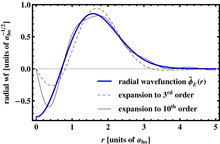
Figure 3: (Color online). The radial wave function $\tilde{\phi}_{E}(r)$ in a spherical harmonic trap introduced in Eq. (5) is compared for the REL energy $E=2.5\hbar\omega$ to its expansion $\phi_{\rm exp}=\sum_{n=0}^{N-1}\langle\phi_{n}|\phi_{E}\rangle\phi_{n}(r)$ to different orders $N$, where $\phi_{n}$ is the radial wave function of the non-interacting system with radial momentum $l=0$ and energy $(2n+\frac{3}{2})\hbar\omega$. Since all non-interacting radial basis functions are zero for $r=0$ the expansion cannot reproduce the behavior of $\tilde{\phi}_{E}(r)$ for $r\rightarrow 0$. This is important, since the coupling to the bound state is proportional to $\tilde{\phi}_{E}^{\prime}(0)$ or $\phi_{\rm exp}^{\prime}(0)$, respectively.

The reason for this insufficiency of the basis to conform to the behavior of a delta-like coupling is related to the problem of a missing coupling of the form $\sqrt{4\pi}\gamma r\delta(\vec{r}\,)$: the two-particle basis states are $a=0$ wave functions. However, $a=0$ basis functions can represent the full wave function only for $r>0$ but not for $r\rightarrow 0$ (see Fig. 3). While for ordinary interaction potentials the value of the wave function at $r=0$ is irrelevant, for zero-range potentials it is decisive. The problem is especially severe for the open-channel bound state, which appears for positive scattering lengths. For $E\rightarrow-\infty$ one has $|\tilde{\phi}_{E}(0)|\propto(-E)^{1/4}$ making its representation by $a=0$ basis functions for decreasing energy more and more problematic.

For weak coupling the problem is less severe as eigenstates that differ significantly from the background trap states are predominantly bound states with different COM excitations, which are well reproduced by the BH model. For strong coupling, however, the bound state is admixed to many states in the spectrum (see Sec. II). Since the bound-state admixture for a certain eigenstate is thus lower, a good representation of the open-channel wavefunction is important also for large scattering lengths.

The described problem does not only arise when using non-interacting $a=0$ basis states. For any finite expansion of the radial wave function $\phi_{\rm exp}(r)=\sum c_{n}\phi_{n}(r)$ in a superposition of basis functions with a specific scattering length $a_{b}$ [i.e. $a_{b}=-\phi_{n}(0)/\phi_{n}^{\prime}(0)$] the scattering length of the expansion yields

$$a_{\rm exp}=-\frac{\phi_{\rm exp}(0)}{\phi_{\rm exp}^{\prime}(0)}=\frac{\sum c_{n}a_{b}\phi_{n}^{\prime}(0)}{\sum c_{n}\phi_{n}^{\prime}(0)}=a_{b}\,.$$ (28)

Hence, the wave function $\phi_{\rm exp}(r)$ cannot adapt to a change of the scattering length induced by a short-range coupling. Especially, since the scattering length at a FR is energy dependent these expansions cannot reproduce the correct eigenenergies and eigenstates.

V Dressing of coupling strength and bound-state energy

To circumvent the problem of the wrong representation of a zero-range coupling one can replace it by a finite-range coupling. To this end one usually considers the Fourier transform of the problem and regularizes the delta-like interaction by introducing a high-momentum cut-off $\Lambda$. Thereupon the coupling parameter is renormalized Cavalcanti (1999). Taking the limit $\Lambda\rightarrow\infty$ the finite-range coupling converges towards a zero-range coupling. However, for an interaction with a range of $d/N$ where $d$ is the lattice spacing more than $N$ Bloch bands have to be included to converge the energies Büchler (2012).

Here we want to take a different approach with no need to include more Bloch bands to reproduce the correct bound-state energies. Provided with the analytic solution in the harmonic trap a dressed bound state is introduced, which reproduces the correct energy spectrum in the harmonic trap at least in the important energy range of the first Bloch band. We use the fact that the full bound state (the combination of the closed-channel and open-channel bound state) falls off rapidly for increasing internuclear separation. Hence, the bound state does hardly probe the anharmonic parts of the potential and the dressed bound state can be equally used for (anharmonic) OLs.

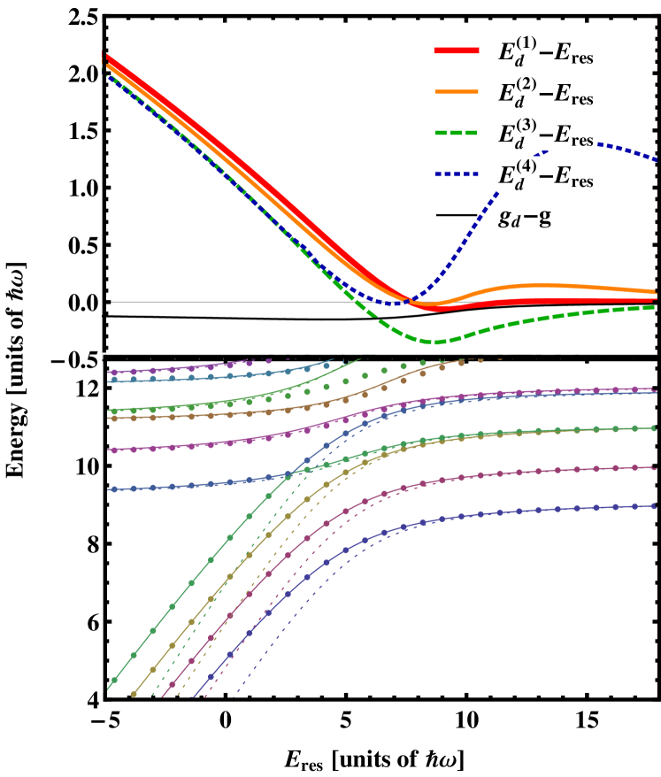
Figure 4: (Color online). Results of the dressed BH model for four Bloch bands with $a_{\rm bg}=0.04a_{\rm ho}$ and $\Delta E=16\hbar\omega$. Top: Dressed bound-state energies and dressed coupling strength as a function of $E_{\rm res}$. Bottom: Comparison of the analytic energy spectrum (dots) with the energies of the dressed BH model (solid lines) and the undressed BH model (dotted lines).

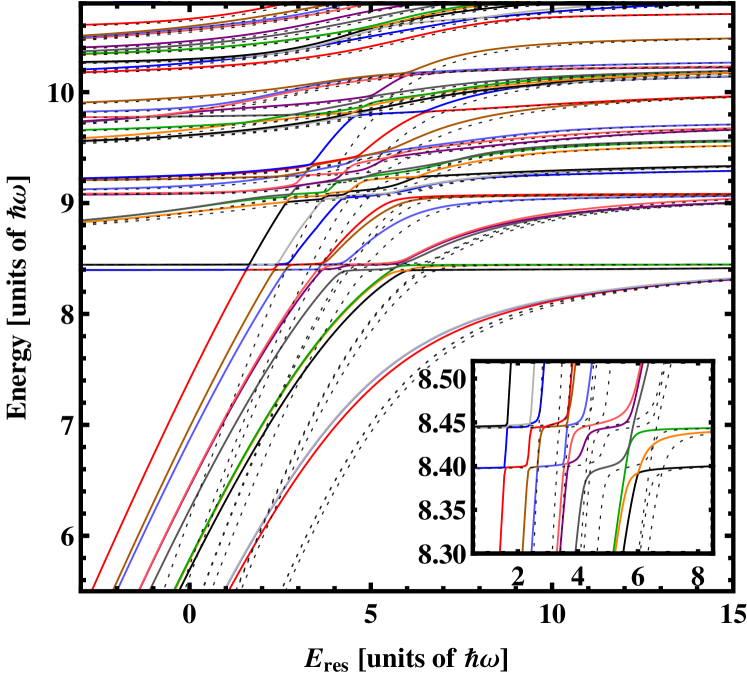
Figure 5: (Color online). Energy spectrum of two atoms in an OL with lattice depth $V_{\rm L}=5E_{r}=1.1\hbar\omega$ consisting of three lattice sites with periodic boundary conditions. Excitations in transversal direction are frozen out by choosing transversal trapping frequencies $\omega_{y}=\omega_{z}=3.8\omega$, where $\omega$ is the frequency of the harmonic approximation of a lattice site in $x$ direction. The resonance parameters are $a_{\rm bg}=85\,\text{a.u.}=9.0\cdot 10^{-3}d$, and $\Delta E=24.2\hbar\omega$ which corresponds to a coupling strength of $\chi=1.66\,\hbar\omega=1.48\,V_{\rm L}$ (See also the right graph in Fig. 9 with the same lattice parameters and resonance parameters). The comparison of the eigenenergies of the dressed BH model (solid lines) and the undressed BH model (dashed lines) each with four Bloch bands included, shows that again both models disagree especially for the bound states, while the differences for the trap states are small. The inset shows a magnification of the spectrum close to the crossing of excited bound states with the lowest Bloch band.

More concretely, the dressed bound state is introduced in the following way: The RBS in the first band (for which the COM wave function is a Wannier function of the first band) couples predominantly to two atoms in the first band leading to the lowest avoided crossing in the spectrum. The two corresponding eigenenergies are given by a sum of the lowest COM energy $E^{\rm\rm COM}_{1}$ [$E^{\rm\rm COM}_{n}=\hbar\omega(n-\frac{1}{2}+\eta)$] and the two lowest solutions $E_{1},E_{2}$ of the REL motion eigenenergy relation (16) which depend on the bound-state energy $E_{b}=E_{\rm res}$. In order to match the energies of this avoided crossing the bound-state energy $E_{b}$ and the coupling strength $g$ are replaced by dressed parameters $E_{b}\rightarrow E_{d}^{(1)}(E_{\rm res})$ and $g\rightarrow g_{d}$. The two parameters are determined by a least square fit to the energies $E_{1}+E_{0}^{\rm\rm COM}$ and $E_{2}+E_{0}^{\rm\rm COM}$.

To match the energies $E_{1}+E_{n}^{\rm\rm COM}$ with $n=2,3,\dots$ of bound states in higher Bloch bands, dressed bound-state energies $E_{d}^{(2)}(E_{\rm res}),E_{d}^{(3)}(E_{\rm res}),\dots$ are introduced, which are also determined by a least square fit. The upper branches of the avoided crossings with bound states in higher Bloch bands lay above the first Bloch band. Therefore, their correct representation is less relevant and we do not need to introduce also band-dependent dressed coupling strengths.

In Fig. 4 the dressed energies $E_{d}^{(1)},E_{d}^{(2)},E_{d}^{(3)},E_{d}^{(4)}$ and $g_{d}$ and the corresponding corrected spectrum are shown for the four-band BH model with $a_{\rm bg}=0.04a_{\rm ho}$ and $\Delta E=16\hbar\omega$ (same parameters as for right bottom graph in Fig. 2). Evidently, the dressing of the bound states becomes relevant for a resonance energy $E_{\rm res}<5\,\hbar\omega$, but is already visible for $E_{\rm res}<10\,\hbar\omega$ . Since only a band-independent dressed coupling strength was introduced, the repulsive branches above the first Bloch band with an energy above $10\hbar\omega$ are not fitted to the exact results. Correspondingly, slight deviations between the exact energies and the dressed BH energies appear for these states, while the first repulsive branch is correctly reproduced.

The introduced dressed parameters can now be used to determine the energy spectrum of two atoms in an OL. In Fig. 5 the spectrum of the dressed and undressed BH model of two atoms in a small OL consisting of three lattice sites are compared for a coupling energy of $\chi=1.66\,\hbar\omega=1.48\,V_{\rm L}$. In contrast to the purely harmonic trap, the energies of the bound states and the trap states split due to tunneling. If the molecular bound states are not in resonance, i.e. for $E_{\rm res}<0$, the trap-state energies form bands of increasing widths around $8.4\hbar\omega$, $9.1\hbar\omega$, $9.8\hbar\omega$, and $10.4\hbar\omega$. For resonance energies $E_{\rm res}>0$ the bound states cross with the trap states leading to a plethora of avoided crossings. In the ultracold regime especially the avoided crossings with the first band are of relevance. These appear due to the next-neighbor coupling of the molecular state with the atomic states von Stecher et al. (2011). As shown in the inset of Fig. 5 the width of these avoided crossings decreases with the COM excitation energy of the RBS. The comparison between the dressed and the undressed BH model shows that also in the OL the energies disagree especially for the bound states, while the energy differences for the trap states are small.

VI Non-perturbative determination of stationary and dynamical states

In the following the results of the BH model shall be compared to non-perturbative calculations for two atoms at a FR in an OL consisting of two lattice sites. In order to do so an approach described in Grishkevich et al. (2011) is used, which allows for finding the stationary solutions of the two-body problem with arbitrary isotropic single-channel interaction potentials. On the basis of the stationary solutions the method described in Schneider et al. (2012) is used to determine the time-dependent wavefunction during a perturbation of the lattice potential.

Since the lattice potential couples REL and COM motion and the interaction couples the motion in $x$, $y$ and $z$ direction all six coordinates of the problem are coupled. An extension to the coupling to an additional channel describing the COM and REL motion of the molecular bound state would make the solution very cumbersome. Instead, the freedom of the choice of the interaction potential is used to realistically mimic a two-channel problem by a square-well interaction potential. The potential supports bound states that are coupled by a barrier to the scattering states. In the following it is shown that this potential leads to an energy dependence of the scattering length, which is in very good agreement to the one of a two-channel description in Eq. (12). This is already sufficient to realistically mimic a FR since, as shown in Sec.II, the energy dependence of the scattering length fully determines the energy spectrum.

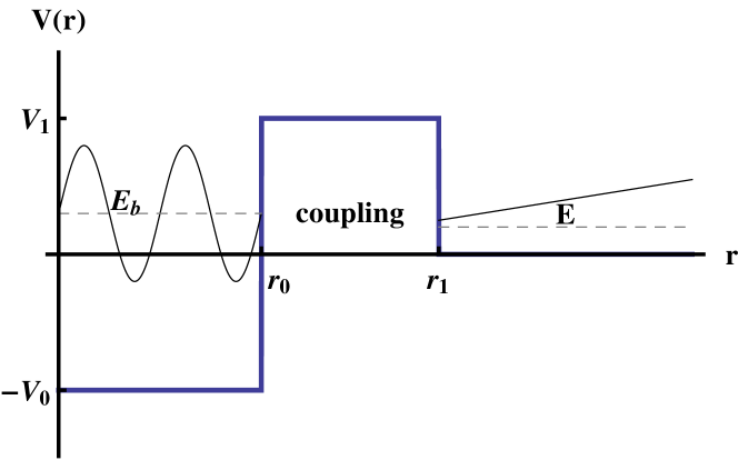
Figure 6: (Color online). Sketch of the square well potential (thick blue). The resonant character of the potential is due to the coupling of a bound state with energy $E_{b}$ (gray dashed) to an unbound state with energy $E$ (gray dashed). The according wave functions are sketched by black thin lines. For $E_{b}\approx E$ the scattering length changes resonantly.

The square-well potential is defined as

$$V(r)=\begin{cases}-V_{0}&\text{for }r\leq r_{0}\\ +V_{1}&\text{for }r_{0}<r\leq r_{1}\\ 0&\text{elsewhere}\\ \end{cases}$$ (29)

with $V_{0},V_{1}>0$ (see Fig. 6). This potential has also been used to study effects of the energy-dependence of the scattering length on the BEC-BCS crossover Jensen et al. (2006). For sufficiently large $V_{0}$ the potential supports a bound state behind a potential barrier of height $V_{1}$ and width $r_{1}-r_{0}$. An atom pair that collides with an energy $E=\hbar^{2}k^{2}/(2\mu)$ scatters resonantly, if $E$ is close to the bound-state energy.

Introducing dimensionless variables $\rho=r/r_{1}$, $d=r_{0}/r_{1}$, $\kappa=kr_{1}$, $v_{0}=V_{0}/E_{0}$, and $v_{1}=V_{1}/E_{0}$ with $E_{0}=\frac{\hbar^{2}}{2\mu r_{1}^{2}}$ the solution of the Schrödinger equation for $E>0$ is given as

$$\phi(\rho)=\begin{cases}C\sin(k_{0}\rho)&\text{ for }\rho<d\\ Ae^{k_{1}\rho}+Be^{-k_{1}\rho}&\text{ for }d\leq\rho<1\\ \sin\left(\kappa\rho+\varphi(k)\right)&\text{ elsewhere, }\end{cases}$$ (30)

with $k_{0}=\sqrt{v_{0}+\kappa^{2}}$ and $k_{1}=\sqrt{v_{1}-\kappa^{2}}$.

In the case of pure $s$-wave scattering one has $\kappa\ll 1$ so that one can make, e.g., the replacements $\sin(\kappa)\rightarrow\kappa$ and $\cos(\kappa)\rightarrow 1$. Eliminating $A,B,$ and $C$ by demanding that the wavefunction is continuous and differentiable the scattering length can be obtained as

$$\frac{a(\kappa^{2})}{r_{1}}\equiv-\frac{\tan\varphi}{\kappa}=\frac{1+\epsilon_{\rm res}}{\epsilon_{\rm res}-\kappa^{2}}$$ (31)

with

$$\epsilon_{\rm res} =k_{1}\frac{\alpha+\beta}{\alpha-\beta},$$ (32)

$$\alpha =e^{2dk_{1}}\left[k_{0}\cos(dk_{0})-k_{1}\sin(dk_{0})\right],$$ (33)

$$\beta =e^{2k_{1}}\left[k_{0}\cos(dk_{0})+k_{1}\sin(dk_{0})\right].$$ (34)

From the functional behavior of Eq. (31) one can determine the corresponding parameters of the FR, i.e. $E_{\rm res}$, $\Delta E$, and $a_{\rm bg}$. The resonance positions of $a(\kappa^{2})$ are given by the roots of $\kappa^{2}=\epsilon_{\rm res}(\kappa^{2})$. The smallest root shall be called $\kappa_{\rm res}^{2}=\epsilon(\kappa_{\rm res}^{2})$. Hence, the resonance position evaluates to

$$E_{\rm res}=E_{0}\kappa_{\rm res}^{2}.$$ (35)

According to Eq. (12) the scattering length is zero if $E=E_{\rm res}-\Delta E$. Be $\kappa_{0}$ the solution of $1+\epsilon_{\rm res}(\kappa_{0})=0$ that is closest to $\kappa_{\rm res}$ then

$$\Delta E=E_{0}(\kappa_{\rm res}^{2}-\kappa_{0}^{2}).$$ (36)

In order to determine the value of the background scattering length $a_{\rm bg}$, $\epsilon_{\rm res}$ is expanded linearly in $\kappa^{2}$ around the resonance position, yielding

$$\epsilon_{\rm res}(\kappa^{2}) \approx \kappa_{\rm res}^{2}+\delta(\kappa^{2}-\kappa_{\rm res}^{2})$$ (37)

$$\text{with}\quad\delta = \left.\frac{\partial\epsilon_{\rm res}}{\partial(\kappa^{2})}\right|_{\kappa=\kappa_{\rm res}}.$$ (38)

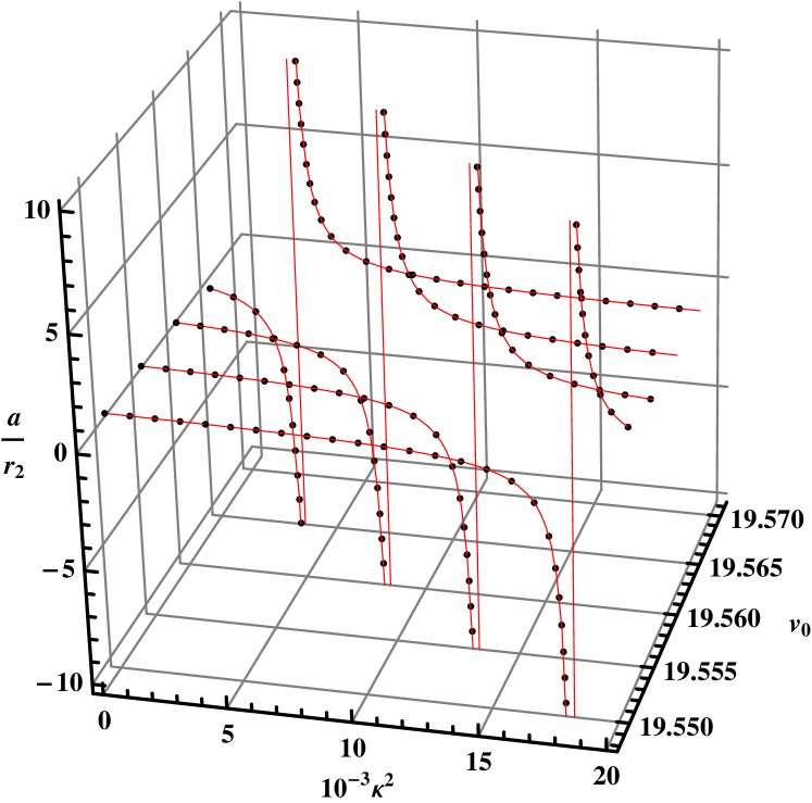
Figure 7: (Color online) Energy-dependent scattering length of the square-well potential (dots) and approximation according to Feshbach theory (thin red) for $v_{1}=70$ and $r_{0}/r_{1}=0.6$.

For $\kappa\rightarrow\kappa_{\rm res}$ the scattering length evaluates according to Eq. (31) and Eq. (37) to

$$\begin{split}\frac{a(\kappa^{2})}{r_{1}}&=\frac{\frac{1}{\delta-1}\left(\kappa_{\rm res}^{2}+1\right)}{\kappa_{\rm res}^{2}-\kappa^{2}}\end{split}$$ (39)

By comparing with the behavior of Eq. (12) for $E\rightarrow E_{\rm res}$, $a=a_{\rm bg}\Delta E/(E_{\rm res}-E)$, one finds

$$a_{\rm bg}=r_{1}\frac{E_{\rm res}+E_{0}}{\Delta E(\delta-1)}\,.$$ (40)

For non-resonant background scattering the wavefunction simply falls off exponentially for $r<r_{1}$. Therefore $a_{\rm bg}\lesssim r_{1}$. Since the potential mimics an $s$-wave resonance, the choice for $r_{1}$ is limited to $kr_{1}\ll 1$ and for energies $E\approx\hbar\omega$ to $r_{1}\ll a_{\rm ho}$, allowing only for rather small positive background scattering lengths. On the other hand, one can freely choose $E_{\rm res}$ and $\Delta E$ by an appropriate choice of the parameters $v_{0}$ and $v_{1}$, respectively. In order to also control the background scattering length one could add another square well with $V<0$ in front of the potential in Eq.(29). However, here the focus lies on the coupling to the RBS and not on the value of $a_{\rm bg}$.

In Fig. 7 $a(\kappa^{2})$ is shown for an exemplary square-well potential with $d=0.6$ and $v_{1}=70$. The values of $a(\kappa^{2})$ according to Eq. (31) and its approximation

$$a=a_{\rm bg}\left(1-\frac{\Delta E}{E_{\rm res}-E}\right)$$ (41)

with the parameters according to the equations (35), (36), and (40) agree almost perfectly, showing that the square-well potential reproduces very well the behavior of a FR.

VII Comparison of Bose-Hubbard model to non-perturbative calculations

VII.1 Energy spectrum

Equipped with the possibility to model FRs with a single-channel potential we can apply the ab-initio approach introduced in Grishkevich et al. (2011) to determine the energy spectrum of two atoms at an FR in a small OL with a lattice spacing of $d=500\;$nm. Within the numerical approach one can expand the OL potential in all directions to some arbitrary order. Again, to avoid unnecessary complexity the OL is expanded to harmonic order around $y=z=0$ in $y$ and $z$ direction and to 12-th order around $x=\pi/2$ in $x$ direction. The lattice depth in $y$ and $z$ direction is chosen sufficiently large ($\omega_{y}=\omega_{z}=3.8\omega$ where $\omega$ is the trap frequency of the harmonic approximation of the lattice wells in $x$ direction) such that excitations in these directions can be ignored. The resulting double-well potential in $x$ direction is shown in Fig. 8.

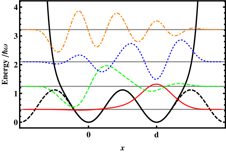
Figure 8: (Color online) Double-well potential (thick, solid) used in the ab initio calculations and corresponding full lattice potential $V_{\rm L}\sin^{2}(k_{0}x)$ (thick, dashed). The Wannier functions of the atoms in the BH model are depicted for bands one to four (red solid, green dashed, blue dotted and orange dot-dashed) alternately for the right and the left well. Already above the first band they clearly probe regions where the double-well potential significantly differs from the full lattice potential. Horizontal lines mark the onsite energies of bands one to four.

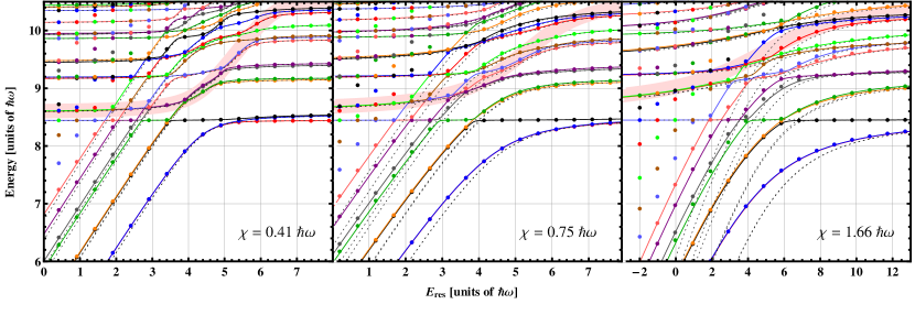
Figure 9: (Color online) Spectra of the ab-initio calculations (dots) and the BH model with usage of the dressed bound-state energies and coupling (lines). Also shown are the energies of the undressed BH model (dotted lines). The ab-initio calculations include the representation of bound states with many COM excitations. Not all of these bound states are present in the BH model that only includes four Bloch bands. For example, in the right graph all ab-initio energies for $7.4\hbar\omega<E<8.4\hbar\omega$ and $E_{\rm res}<0$ are not covered by the BH model. From left to right the parameters $a_{\rm bg}=(88,87,85)\,\text{a.u.}=(9.3,9.2,9.0)\cdot 10^{-3}d$, $\Delta E=(1.4,4.9,24.2)\hbar\omega$ are chosen. This corresponds to a coupling strength of $\chi=(0.41,0.75,1.66)\,\hbar\omega=(0.36,0.67,1.48)\,V_{\rm L}$. The red shading marks the energy of the repulsively interacting atoms within a single-band approximation. From left to right the energy of this state is significantly influenced by the bound state in the second, third and fourth Bloch band demonstrating that for stronger coupling bound states in more Bloch bands have to be included to obtain accurate eigenenergies.

For large lattice depths the spectrum converges to the one of two uncoupled harmonic traps. In order to probe the accuracy of the BH model a relatively small lattice depth of $V_{\rm L}=5E_{r}=1.1\hbar\omega$ is chosen in $x$ direction. For this low lattice depth excited states in higher Bloch bands probe parts of the potential that significantly deviate from an ordinary lattice potential $V_{\rm L}\sin^{2}(k_{0}x)$. Therefore, the correct single-atom states deviate significantly from ordinary Wannier functions. This insufficiency can be corrected for by replacing the ordinary Wannier basis by a basis constructed from single-atom eigenstates in the double well. For each band $p$ the left and right Wannier functions are constructed by superpositions of the $n$-th symmetric eigenstate with energy $E_{p}^{(\rm even)}$ and the $n$-th anti-symmetric eigenstate with energy $E_{n}^{(\rm odd)}$. The corresponding atomic Wannier functions of the first four Bloch bands are shown in Fig. 8. As one can see they are neither symmetric nor anti-symmetric so that any selection rule for the BH parameters (such as that of the coupling between the open and the closed channel) of the OL does not apply. The onsite energies are given as $\epsilon_{n}=\frac{1}{2}(E_{n}^{(\rm odd)}+E_{n}^{(\rm even)})$ and the hopping parameters as $J_{n}=\frac{1}{2}(E_{n}^{(\rm odd)}-E_{n}^{(\rm even)})$. Furthermore, to be sure that all errors are solely due to deficiencies of the representation of the Feshbach resonance in the BH model also next-neighbor (background) interaction is included.

In Fig. 9 the spectrum of the ab-initio calculation for three different coupling strengths is compared to the corresponding dressed and non-dressed BH spectrum. In contrast to Fig. 5 the trap states do not appear in energy bands due to the reduced size of the system. The bound states appear as duplets with one symmetric and one antisymmetric COM excitation in $x$ direction. Again, excited bound states in higher Bloch bands are able to couple to the first trap state (lowest horizontal line) by next-neighbor coupling, i.e. the bound state couples to a state of one atom in the same well and one in the neighboring well. For symmetry reasons only the lower bound state of each dublet can couple to the lowest symmetric trap state von Stecher et al. (2011).

Fig. 10 shows a detailed view onto two of these avoided crossings around $E=8.4\hbar\omega$ for a resonance energy of $E_{\rm res}=2.9\hbar\omega$ and $E_{\rm res}=3.9\hbar\omega$. Clearly, the splitting of the avoided crossing and hence also the next-neighbor coupling strength is well reproduced by the dressed BH model.

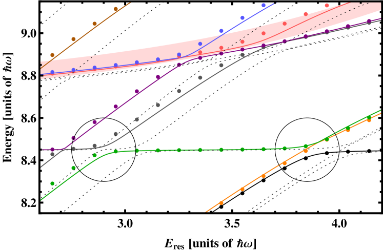
Figure 10: (Color online) Zoom on the resonance of the bound state in the second Bloch band (right circle) and third Bloch band (left circle) with the state of two separated atoms in the ground state for $\chi=0.75\hbar\omega$. The splitting energies of the left resonance ($0.04\hbar\omega$) and that of the right resonance ($0.06\hbar\omega$) are well reproduced by the dressed BH models.

Given the large degree of anharmonicity of the lattice potential the agreement between the ab-initio spectra and BH spectra in Figs. 9 and 10 is very good. The dressed bound-state energies are obtained from a harmonic approximation of the two lattice sites. Already in the second Bloch band the potential and therefore the states and energies differ significantly from their harmonic counterparts (see Fig. 8). Nevertheless, the dressed bound-state energies and the dressed coupling strength lead to a drastic improvement of the undressed results in all three cases shown in Fig. 9. In general, the dressed parameters should lead to an improvement as long as the couplings of the bound states to trap states that probe anharmonic parts of the potential, i.e. with energies above $E=V_{\rm L}$, is negligible. Approximately, for $\chi\geq V_{\rm L}$ this is not the case any more since at the avoided crossing of the lowest bound state with the lowest trap state an energy regime above $V_{\rm L}$ is entered. Indeed, considering the spectrum with the largest coupling energy $\chi=1.48V_{\rm L}=1.66\hbar\omega$, the lowest bound-state energy of the BH model is slightly lower than that of the ab-initio calculations. But still the disagreement is surprisingly small. As one can expect the correction of the bound-state energies in the third and fourth Bloch band is less accurate than that of the first and second Bloch band. Already for the lower coupling energies of $\chi=0.36V_{\rm L}=0.41\hbar\omega$ and $\chi=0.67V_{\rm L}=0.75\hbar\omega$ small disagreements between the corresponding eigenenergies of the ab-initio calculations and the corrected BH model appear.

The coupling of the two atoms in the lowest Bloch band to the bound state in the lowest Bloch band leads to the appearance of both attractively and repulsively interacting states. The energy of the repulsively interacting state is marked by the red shading in Figs. 9 and  10. As one can see for larger and larger coupling energy $\chi$ this state is strongly influenced by bound states in higher and higher Bloch bands. If this energy range shall be correctly reproduced this sets a lower limit for the number of Bloch bands that must be included in the BH model. In Fig. 10 one can see that the dressed BH model reproduces correctly the energy of the repulsively interacting state while the undressed model underestimates its energy.

As discussed above, the dressed BH model reproduces accurately the correct eigenenergies up to coupling energies $\chi\sim V_{\rm L}$. This corresponds usually to small up to medium FRs. As discussed in Sec. II a FR in a harmonic trap is broad if $a_{\rm bg}\Delta E\gg a_{\rm ho}\hbar\omega$. Since $\chi$ is a measure for the energy splitting of the avoided crossing of the lowest bound state with the first band, it is comparable to $\sqrt{a_{\rm bg}\Delta E/(a_{\rm ho}\hbar\omega)}\hbar\omega$ in the harmonic trap. Therefore, a broad resonance requires $[\chi/(\hbar\omega)]^{2}\gg 1$. Since the BH model is valid for $\chi\sim V_{\rm L}$ it can only accurately describe broad FRs in a very deep lattice with $(V_{\rm L}/(\hbar\omega))^{2}=V_{\rm L}/(4E_{r})\gg 1$.

However, for broad FRs all details of the interaction apart from the value of the scattering length for $E\rightarrow 0$ are irrelevant (see Sec. II). In this situation there is not required to explicitly include the bound state in the BH model. Instead, corrected BH models like the one introduced in Schneider et al. (2009) already provide accurate results.

VII.2 Time-dependent manipulations

In the following it is studied how well the BH model can predict the dynamic behavior of the system under the influence of some time-dependent perturbation

$$\hat{\rm V}_{\rm pert}(t)=\sum_{i=1}^{M}v_{\rm pert}(\vec{r}_{i}\,)f(t)\,,$$

which acts on each of $M$ identical atoms in the same way.

Normally, any external potential $v_{\rm pert}(\vec{r}_{i})$ is approximately constant on the length scale of the bound state. Hence, the perturbation cannot couple the orthogonal closed and open channel states. The matrix elements of the perturbation of the closed channel evaluate to

$$\begin{split}&\left<\psi_{b}\tilde{w}_{i,n}\right|\sum_{i=1}^{M}v_{\rm pert}(\vec{r}_{i}\,)\left|\tilde{w}_{j,m}\psi_{b}\right>=\int d\vec{R}\;\int d\vec{r}\;|\psi_{b}(\vec{r}\,)|^{2}\times\\ &\times\tilde{w}_{i,n}(\vec{R})\left[v_{\rm pert}\left(\vec{R}+\frac{1}{2}\vec{r}\right)+v_{\rm pert}\left(\vec{R}-\frac{1}{2}\vec{r}\right)\right]\tilde{w}_{j,m}(\vec{R})\\ &\approx\int d\vec{R}\;\tilde{w}_{i,n}(\vec{R})\int d\vec{r}\;|\psi_{b}(\vec{r}\,)|^{2}\;2v_{\rm pert}(\vec{R})\tilde{w}_{j,m}(\vec{R})\\ &=2\left<\tilde{w}_{i,n}\right|\hat{\rm v}_{\rm pert}\left|\tilde{w}_{j,m}\right>\end{split}$$

Hence, in second quantization the perturbation is expressed as

$$\begin{split}\hat{\rm V}_{\rm pert}(t)=f(t)\bigg{(}&\sum_{\left<i,j\right>}\sum_{n,m=1}^{N}\left<w_{i,n}\right|\hat{\rm v}_{\rm pert}\left|w_{j,m}\right>a_{i,n}^{\dagger}a_{j,m}\\ &+2\sum_{\left<i,j\right>}\sum_{n,m=1}^{N}\left<\tilde{w}_{i,n}\right|\hat{\rm v}_{\rm pert}\left|\tilde{w}_{j,m}\right>b_{i,n}^{\dagger}b_{j,m}\bigg{)}\end{split}$$

As usual, only next-neighbor coupling and on-site coupling are considered and the basis is restricted to the first $N$ Bloch bands.

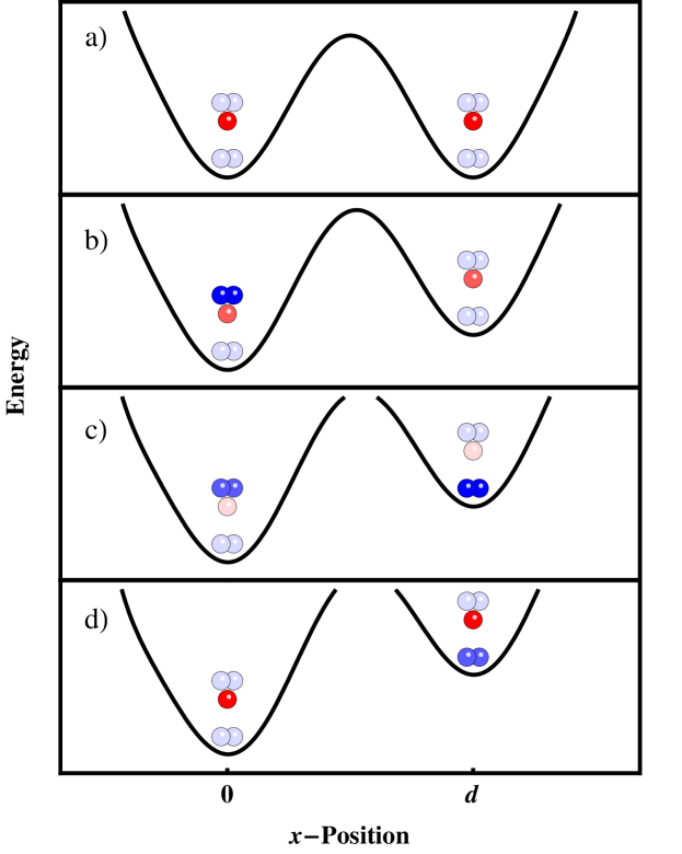
Figure 11: (Color online) Sketch of the dynamical behavior while accelerating (inclining) the double-well. a) The initial state consists of separated atoms (red disks) in the ground state of the left and right well. The four molecular states in the COM ground state (blue double disk below red disks) and in the first excited COM state (blue double disk above red disks) are not in resonance. b) Upon inclining the potential the energy of an excited molecular state in the left well (dark blue) comes in resonance with the energy of the separated atoms. The molecular state is occupied and the COM of the system moves to the left. c) After a further inclination the energy of the excited molecule in the left well comes into resonance with the ground-state molecule in the right well. By occupying this state the COM of the system moves to the right. d) Finally, the molecule on the right well comes into resonance with the initial state of two separated atoms and the COM of the system moves again to the left.

In the following, the case of a linear perturbation with increasing strength,

$$\hat{\rm V}_{\rm pert}(t)=\sum_{i=1}^{N}\hat{x}_{i}\lambda t\quad,$$

is considered, which corresponds to an increasing acceleration of the lattice Schneider et al. (2012). The dynamical behavior due to $\hat{\rm V}_{\rm pert}$ is governed mainly by two effects: (i) The linear perturbation leads to a coupling between Wannier functions of odd and even symmetry, i.e. between bands with odd and even quantum numbers. (ii) The energy of the states at each lattice site are shifted proportionally to the product $\lambda dj$ and thus depend on the site number $j$.

Of course, the dynamical behavior also strongly depends on the value of the resonance energy $E_{\rm res}$. For the dynamical studies a resonance energy is chosen such that an inclination leads to the resonant next-neighbor coupling of two separated atoms in the ground state to a bound state in the first and second Bloch band. The corresponding dynamical behavior is sketched in Fig. 11. As one can see the COM movement of the system upon accelerating the lattice depends crucially on the resonance energy, i.e. the energy of the RBS. Depending on the bound state and its COM excitation that comes into resonance the system can move against the direction or in direction of the acceleration. A precise representation of the system is thus necessary to predict the mobility behavior of two atoms at a Feshbach resonance.

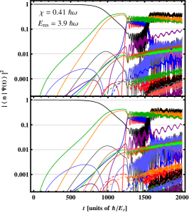
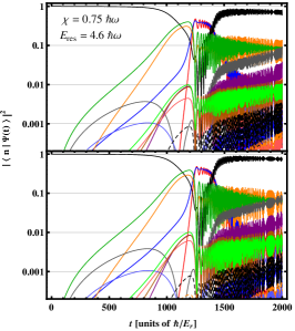
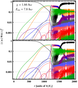
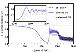
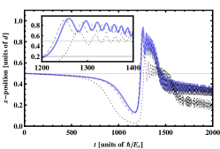
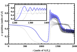
Figure 12: (Color online) Dynamic behavior of two separated atoms in the ground state of the double-well potential during an inclination of the lattice for different coupling energies $\chi$ and resonance energies $E_{\rm res}$. At $t=t_{\rm end}=2000\hbar/E_{r}$ each atom experiences a perturbation of $\hat{\rm W}=0.7\hbar\omega\hat{x}/d$ which suffice to bring both the first and second bound state into resonance (see Fig. 11). The projection of the time-dependent wave function $\left|\Psi(t)\right>$ onto the eigenstates $\left|n\right>$ of the unperturbed system is shown in the first row (ab-initio results) and the second row (results of the dressed BH model) using the same color coding as in Figs. 9 and 10. In the lowest row the mean COM position $\left<\Psi(t)\right|\hat{X}\left|\Psi(t)\right>$ is shown for the ab initio results and the dressed and undressed BH model. The insets show a magnified region of the beginning of the fast oscillations between $1200\hbar/E_{r}$ and $1400\hbar/E_{r}$.

Fig. 12 shows the projections $|\left<n\vphantom{\Psi(t)}\right|\left.\Psi(t)\vphantom{n}\right>|^{2}$ of the time-dependent wavefunctions $\left|\Psi(t)\right>$ onto the eigenstates $\left|n\right>$ of the unperturbed system for a slow inclination with $\lambda=0.0003\frac{E_{r}}{\hbar}\frac{\hbar\omega}{d}$. If the perturbation would be suddenly switched off, the projections give the probability of finding the system in the corresponding eigenstate. For the same three coupling energies as shown in Fig. 9 the qualitative agreement between the result of the ab-initio approach (upper row) and the dressed BH model (middle row) is very good. As is visible in Fig. 11, initially the bound state in the second Bloch band is slowly occupied. After $t\approx 1300\hbar/E_{r}$ this bound state gets into resonance with the bound state in the first Bloch band which is then occupied. After $t\approx 1500\hbar/E_{r}$ the main occupation moves back to the initial state. Additionally to the behavior described in Fig. 11 the inclination leads to a strong coupling of the bound states in the first and second Bloch bands on each lattice site. Due to the large energy separation of these states this coupling leads to fast oscillations of the population of the eigenstates.

In order to examine the quantitative agreement between the ab-initio and dressed BH results the time-dependent COM motion of the system $\left<\Psi(t)\right|\hat{X}\left|\Psi(t)\right>$ has been determined. As one can see in the lower row in Fig. 11 the quantitative agreement is very good for the smallest coupling energy $\chi=0.41\hbar\omega$. For the larger coupling energies especially the fast oscillations appearing after $t\approx 1200\hbar/E_{r}$ are less accurately reproduced by the dressed BH model. The phase shift and altered frequency of the oscillations is mainly due to a small underestimation by about 1% of the coupling strength between the stationary eigenstates within the dressed BH model. In contrast to the dressed BH model, the undressed BH model leads even for small coupling energies to a dynamical behavior significantly disagreeing from the one of the ab-initio calculations.

VIII Conclusion

We have introduced a Bose-Hubbard model with dressed bound states and a dressed coupling strength, which can be used to accurately determine the stationary and dynamical wavefunctions of two atoms in an optical lattice at a Feshbach resonance. The dressed parameters, which can be straightforwardly obtained from the analytically known solution of a Feshbach resonance in a harmonic trap, allow one to obtain an accurate solution with including only a small number of Bloch bands. The dressing avoids the problem that the eigenenergies, obtained by a finite expansion of the solution in single-atom basis states, do not converge to the correct eigenenergies in the presence of a delta-like coupling to the bound state. Hence, the introduced method permits to determine accurate solutions without a regularization of the potential and a numerically demanding expansion of the solution, e.g., in Bloch functions or Wannier functions of many Bloch bands. The solution of this problem should be relevant to many approaches that seek to describe strongly interacting atoms via a multi-band Hubbard model.

Comparisons to eigenenergies and time-dependent wavefunctions obtained from a non-perturbative approach have shown that the method is accurate as long as the coupling energy is smaller or comparable to the lattice depth. Furthermore, we have described a possibility to realistically mimic FRs within non-perturbative single-channel approaches by using a square-well interaction potential.

We believe that the approach is applicable not only to optical lattices but to various kinds of anharmonic trapping potentials. The introduced methods should be therefore a valuable tools for investigating the exciting physics of Feshbach-interacting atoms in various potentials and to interpret corresponding experimental findings.