Probability-constrained Power Optimization for Multiuser MISO Systems with Imperfect CSI: A Bernstein Approximation Approach

Abstract

We consider power allocations in downlink cellular wireless systems where the basestations are equipped with multiple transmit antennas and the mobile users are equipped with single receive antennas. Such systems can be modeled as multiuser MISO systems. We assume that the multi-antenna transmitters employ some fixed beamformers to transmit data, and the objective is to optimize the power allocation for different users to satisfy certain QoS constraints, with imperfect transmitter-side channel state information (CSI). Specifically, for MISO interference channels, we consider the transmit power minimization problem and the max-min SINR problem. For MISO broadcast channels, we consider the MSE-constrained transmit power minimization problem. All these problems are formulated as probability-constrained optimization problems. We make use of the Bernstein approximation to conservatively transform the probabilistic constraints into deterministic ones, and consequently convert the original stochastic optimization problems into convex optimization problems. However, the transformed problems cannot be straightforwardly solved using standard solver, since one of the constraints is itself an optimization problem. We employ the long-step logarithmic barrier cutting plane (LLBCP) algorithm to overcome difficulty. Extensive simulation results are provided to demonstrate the effectiveness of the proposed method, and the performance advantage over some existing methods.

I Introduction

The multiuser multiple-input single-output (MISO) system can be used to model a communication system where there is an asymmetry between the transmitters and the receivers in terms of the number of antennas employed. For example, in a cellular system, typically the basestation can be equipped with multiple antennas, whereas the mobile users are equipped with single-antennas. Then for the downlink transmission, when a single cell is considered, we have a MISO broadcast channel; whereas when multiple cells are considered, we have a MISO interference channel. Such multiuser MISO channels have been extensively studied in the literature. In particular, the achievable rate regions of the MISO interference channels have been investigated in [1] [2]. In [3] [4], the problem of maximizing the sum rate of the MISO broadcast channel is treated. The same problem is also considered in [5], with the additional max-min fairness constraint. Moreover, bargaining based game-theoretic solutions are given in [6] for a two-user MISO interference channel, and in [7] for the general $K$-user case. All these works assume that perfect channel state information (CSI) is available at the transmitters.

However, in practice, due to various reasons, such as estimation/quantization errors, delayed estimation, and limited feedback rate, the assumption of perfect CSI at the transmitter is unrealistic. In the case of imperfect CSI, the naive approach of treating the imperfect CSI as if it was perfect gives rise to non-robust design, which leads to rapid performance degradation with the increasing error levels [8]. Motivated by this fact, a number of efforts have addressed robust approaches that can cope with uncertainties in the channel knowledge. Convex optimization techniques are important tools for obtaining computationally efficient (exact or approximate) solutions to the robust design problems [9].

Current robust design schemes can be classified into the worst-case and stochastic approaches. In the worst-case analysis [10][11][12][13] [14], the channel uncertainty is considered as deterministic and norm bounded. The worst-case-based optimization approaches provide robustness against CSI imperfections. However, the actual worst case may occur with a very low probability. Hence, the worst-case approach may be overly pessimistic and therefore, may lead to unnecessary performance degradation. The resulting optimization problem sometimes does not even have a feasible solution. Even if the problem is feasible, the resource utilization is inefficient as most system resources must be dedicated to provide guarantees for the worst-case scenarios.

To provide more flexibility than the worst-case designs, the outage-probability-constrained robust designs have also been recently developed [15] [16] [17][18] [19] [20][21][22][23] where the convex optimization tools are employed to solve the resulting stochastic optimization (also referred to as probabilistic programming) problems. In these less conservative approaches the channel state and channel uncertainty are considered as random processes. Compared to the worst-case approach, the stochastic approach achieves better average performance while keeping the probability of the worst performance low. Unfortunately, probability-constrained stochastic optimization are known to be computationally intractable except for a few special cases. In general, such optimizations are difficult to solve as their feasible sets are often nonconvex. In fact, finding feasible solutions to a generic probability-constrained program is itself a challenging research problem in the operations research community.

In this paper, we consider several power allocation problems in multiuser MISO channels with imperfect CSI. We assume that the multi-antenna transmitters employ some fixed beamformers to transmit the data and we focus on optimizing the transmit powers of different users. In particular, for MISO interference channels, we treat two closely related optimization problems: one is to minimize the total transmit power subject to the SINR outage constraints, and the other is to maximize the achievable SINR margin under the power constraint. For MISO broadcast channels, we treat the MSE-constrained power minimization problem. All these problems are formulated as probability-constrained stochastic optimization problems. The major challenge in the stochastic optimization based method is to replace the probabilistic constraints with deterministic ones. We make use of the Bernstein approximation technique, which is a recent advance in the field of probability-constrained programming [24], to transform the probabilistic constraints into deterministic constraints that are conservative. The stochastic optimization problems are then transformed into convex optimization problems.

The remainder of this paper is organized as follows. In Section II, we formulate the Probability-constrained power optimization problems in MISO interference channels. In Section III, we propose solutions to the stochastic optimization problems based on the Berstein approximation technique and the long-step logarithmic barrier cutting plane (LLBCP) algorithm. In Section IV, we treat the MSE-constrained stochastic power optimization problem for MISO broadcast channels. Section IV presents the simulation results and finally, conclusions are drawn in Section V.

II Power Control for MISO Interference Channels with Imperfect CSI

II-A System Model

We consider a MISO interference channel with K transmitters and K receivers. Each transmitter employs $M$ transmit antennas and each receiver is equipped with a single receive antenna. We assume that all receivers treat co-channel interference as noise, i.e., they make no attempt to decode the interference. Assuming a narrowband channel model, the received signal at receiver $k$ is given by

$$y_{k}=\mbox{\boldmath$h$}_{kk}^{H}\mbox{\boldmath$x$}_{k}+\sum_{j\neq k}\mbox{\boldmath$h$}_{kj}^{H}\mbox{\boldmath$x$}_{j}+n_{k}$$ (1)

where $\mbox{\boldmath$x$}_{k}\in{\mathbb{C}}^{M}$ is the transmitted signal vector by the $k$-th transmitter, $\mbox{\boldmath$h$}_{kj}\in{\mathbb{C}}^{M}$ is the vector of complex channel gains between the j-th transmitter and the k-th receiver, $n_{k}\sim{\cal N}_{c}(0,\eta_{k}^{2})$ is the complex Gaussian noise sample.

We assume that each transmitter employs the beamforming technique to transmit information; that is, we have $\mbox{\boldmath$x$}_{k}=\mbox{\boldmath$w$}_{k}s_{k}$, where $\mbox{\boldmath$w$}_{k}\in{\mathbb{C}}^{M}$ is the transmit beamformer for the link between the k-th transmitter and the k-th receiver, and $s_{k}\in{\mathbb{C}}$ denotes the complex data symbol intended for the k-th receiver.

In practice, the channel state information (CSI) at the receiver or transmitter is imperfect, especially for the transmitter-side CSI. In this paper, we assume that the transmitter only has access to the imperfect CSI to form the beamforming vectors. Specifically, we have the following uncertainty model for the channel vectors

$$\mbox{\boldmath$h$}_{kj}=\mbox{\boldmath$\hat{h}$}_{kj}+{\mbox{\boldmath$\delta$}}_{kj}$$ (2)

where $\mbox{\boldmath$\hat{h}$}_{kj}=\left[{\hat{h}_{kj}^{1},...,\hat{h}_{kj}^{M}}\right]^{T}$ denotes the imperfect estimate of the actual channel vector $\mbox{\boldmath$h$}_{kj}$, and $\mbox{\boldmath$\delta$}_{kj}=\left[{\delta_{kj}^{1},...,\delta_{kj}^{M}}\right]^{T}$ denotes the channel error vector, where

$$\delta_{kj}^{m}\stackrel{{\scriptstyle\mbox{\small{i.i.d.}}}}{{\sim}}\mathcal{N}_{c}\left(0,\sigma_{kj}^{2}\right).$$ (3)

In order to obtain robust solutions that are less sensitive to channel uncertainties, we need to explicitly take into account the impefect CSI. However, the mathematical problem arising from the robust beamformer design is in general much more complicated than the conventional non-robust design. Thus some simplifications are needed to make the problem tractable. In this paper, following [17, 10], we assume that the transmit beamformer is of the form $\mbox{\boldmath$w$}_{k}=p_{k}\mbox{\boldmath$g$}_{k}$, where $p_{k}\in{\mathbb{R}}^{+}$ denotes transmit power, and $\mbox{\boldmath$g$}_{k}=[g_{k}^{1},...g_{k}^{M}]^{T}\in{\mathbb{C}^{M}}$ denotes the unit-norm beamforming vector, i.e., $||\mbox{\boldmath$g$}_{k}||_{2}=1$. Here $\mbox{\boldmath$g$}_{k}$ depends only on the estimated channels and it is designed in a non-robust way. For example, in the channel-matching approach, we have $\mbox{\boldmath$g$}_{k}=\mbox{\boldmath$\hat{h}$}_{kk}$. On the other hand, the design of the power allocation $p_{k}$ is much more sophisticated and it depends not only on the channel estimates, but also on the channel error statistic. In this paper, we assume that the beam directions $\{\mbox{\boldmath$g$}_{k}\}$ are fixed and focus on the power allocation problem.

II-B Problem Formulations

We next formulate the robust power allocation problem based on the outage probability. Our goal is to optimize the system performance through power allocation. The system performance is usually quantified by its quality of service (QoS) and the resources it uses. The most common QoS metrics are the symbol error rate or the achievable data rate, both of which are functions of the output SINRs. The system resources include the transmit power and bandwidth. We consider two probability-constrained optimization problems as follows.

II-B1 SINR-constrained power minimization

The first strategy seeks to minimize the average transmit power subject to the QoS constraints. Given an acceptable SINR level $\alpha_{k}$ and the outage probability $\varepsilon_{k}$ for the k-th transmitter and receiver pair, we aim to minimize the average transmit power while meeting the SINR outage constraints of all users, i.e.,

$$\mathop{\min}\limits_{\left\{{{p_{k}}}\right\}_{k=1}^{K}} \sum\limits_{k=1}^{K}{{p_{k}}}$$

$${\rm s.t.}\ \ \Pr\left({{\Gamma_{k}}\leqslant{\alpha_{k}}}\right)\leqslant{\varepsilon_{k}},\ \ k=1,...,K$$

$${p_{k}}\geqslant 0,\ k=1,...,K$$

where $\mathrm{Pr}(A)$ denotes the probability of the event $A$, and ${\Gamma_{k}}$ denotes the SINR at the k-th receiver, given by

$${\Gamma_{k}}=\frac{{{p_{k}}{{\left|{{\mbox{\boldmath$h$}_{kk}^{H}}{\mbox{\boldmath$g$}_{k}}}\right|}^{2}}}}{{\eta_{k}^{2}+\sum\limits_{j\neq k}{{p_{j}}{{\left|{{\mbox{\boldmath$h$}_{kj}^{H}}{\mbox{\boldmath$g$}_{j}}}\right|}^{2}}}}}$$

The design parameters $\varepsilon_{k}$ ensures that receiver $k$ is served with an SINR no less than $\alpha_{k}$ at least $(1-\varepsilon_{k})\times 100\%$ of the time.

II-B2 Max-Min SINR optimization

The second strategy is to maximize the minimum SINR among all receivers, subject to the SINR outage constraints, and the individual transmit power constraints. We have the following optimization problem.

$$\mathop{\max\min}\limits_{\left\{{{p_{k},\alpha_{k}}}\right\}_{k=1}^{K}} {\alpha_{k}}$$

$${\rm s.t.} \Pr\left({{\Gamma_{k}}\leqslant\alpha_{k}}\right)\leqslant{\varepsilon_{k}},\ k=1,...,K$$

$$0\leqslant{p_{k}}\leqslant{{\bar{p}}_{k}},\ k=1,...,K$$

where ${\bar{p}}_{k}$ is the given power constraint for the k-th transmitter.

Note that the problem in (II-B2) involves the individual power constraint. Alternatively we can also consider the total power constraint to have the following optimization problem.

$$\mathop{\max\min}\limits_{\left\{{{p_{k},\alpha_{k}}}\right\}_{k=1}^{K}} {\alpha_{k}}$$

$${\rm s.t.} \Pr\left({{\Gamma_{k}}\leqslant\alpha_{k}}\right)\leqslant{\varepsilon_{k}},\ k=1,...,K$$

$${p_{k}}\geqslant 0,\ k=1,...,K$$

$$\sum_{k=1}^{K}{p_{k}}\leqslant{{\bar{p}}_{tot}}$$

where ${\bar{p}}_{tot}$ is the maximum allowable total transmit power.

II-C Background on Bernstein Approximation

In problems (II-B1), (II-B2), and (II-B2), the probabilistic constraints make the optimization highly intractable. The main reason is that the convexity of the feasible set corresponding to the probabilistic constraints is difficult to verify. To circumvent the above hurdles, we make use of the Bernstein approximation technique [24] to convert the probabilistic constraints to convex constraints. Next we briefly introduce the Bernstein approximation.

Suppose that $F(\mbox{\boldmath$z$},\mbox{\boldmath$\zeta$}):\mathbb{R}^{n}\times\mathbb{R}^{d}\rightarrow\mathbb{R}$ is a function of $\mbox{\boldmath$z$}\in\mathbb{R}^{n}$ and $\mbox{\boldmath$\zeta$}\in\mathbb{R}^{d}$. Then the probabilistic constraint

$$\mathrm{Pr}\{F(\mbox{\boldmath$z$},\mbox{\boldmath$\zeta$})\geq 0\}\leq\ \varrho$$ (7)

can be conservatively approximated by the following

$$\mathrm{inf}_{t>0}\;\;\{t{\mathbb{E}}\{\psi[t^{-1}F(\mbox{\boldmath$z$},\mbox{\boldmath$\zeta$})]\}-t\varrho\}\leq 0,$$ (8)

or

$$\mathrm{inf}_{t>0}\;\;\{t\log{\mathbb{E}}\{\psi[t^{-1}F(\mbox{\boldmath$z$},\mbox{\boldmath$\zeta$})]\}-t\log\varrho\}\leq 0.$$ (9)

where $\psi:\mathbb{R}\rightarrow\mathbb{R}$ be a nonnegative valued, nondecreasing, convex function satisfying $\psi(z)>\psi(0)=1$ for any $z>0$. For example, $\psi(z)=\exp(z)$. Moreover, assume that for every $\mbox{\boldmath$\zeta$}\in\mathbb{R}^{d}$ the function $F(\cdot,\mbox{\boldmath$\zeta$})$ is convex. Then $t{\mathbb{E}}\{\psi[t^{-1}F(\mbox{\boldmath$z$},\mbox{\boldmath$\zeta$})]\}-t\varrho$ is convex, and thus (8) is convex. Indeed, since $\psi(\cdot)$is nondecreasing and convex and $F(\cdot,\mbox{\boldmath$\zeta$})$is convex, it follows that $(z,t)\rightarrow t\psi(t^{-1}F(z,\mbox{\boldmath$\zeta$}))$ is convex. This, in turn, implies convexity of the expected value function ${\mathbb{E}}\{\psi[t^{-1}F(\mbox{\boldmath$z$},\mbox{\boldmath$\zeta$})]\}$, and hence convexity of $t{\mathbb{E}}\{\psi[t^{-1}F(\mbox{\boldmath$z$},\mbox{\boldmath$\zeta$})]\}-t\varrho$. Similarly, $t\log{\mathbb{E}}\{\psi[t^{-1}F(\mbox{\boldmath$z$},\mbox{\boldmath$\zeta$})]\}-t\log\varrho$ is convex, and thus (9) is convex.

As an important special case, suppose that $\zeta$ is a random vector whose components are independent and nonnegative. $F(\mbox{\boldmath$z$},\mbox{\boldmath$\zeta$})$ is affine in $\zeta$, i.e.,

$$F(\mbox{\boldmath$z$},\mbox{\boldmath$\zeta$})=f_{0}(\mbox{\boldmath$z$})+\sum_{j=1}^{d}\zeta_{j}f_{j}(\mbox{\boldmath$z$}),$$ (10)

and the functions $f_{j}(\mbox{\boldmath$z$}),j=0,1,...,d$, are well defined and convex on $\mathbb{R}^{n}$. Then the probabilistic constraint (7) can be conservatively approximated by (11).

$$\mathrm{inf}_{t>0}\;\;\{t\log{\mathbb{E}}\{\exp[t^{-1}F(\mbox{\boldmath$z$},\mbox{\boldmath$\zeta$})]\}-t\log\varrho\}=\mathrm{inf}_{t>0}\;\;\{f_{0}(\mbox{\boldmath$z$})+\sum_{j=1}^{d}t\log\mathbb{E}\{\exp[t^{-1}\zeta_{j}f_{j}(\mbox{\boldmath$z$})]\}-t\log\varrho\}\leq 0.$$ (11)

Furthermore, the constraint in (11) is convex. To see this, define

$$\begin{gathered}\Psi(\mbox{\boldmath$\gamma$})\triangleq\log(\mathbb{E}[\exp\{\gamma_{0}+\sum_{j=1}^{d}\zeta_{j}\gamma_{j}\}])\hfill\\ \;\;\;\;\;\;\;\;\;=\gamma_{0}+\sum_{j=1}^{d}\log\mathbb{E}[\exp(\zeta_{j}\gamma_{j})].\hfill\\ \end{gathered}$$ (15)

Then (8) can be written as

$$\mathrm{inf}_{t>0}\;\;\{t\Psi(t^{-1}\mbox{\boldmath$f$}(\mbox{\boldmath$z$}))-t\log\varrho\}\leq 0.$$ (16)

The function $G(\mbox{\boldmath$\gamma$},t)\triangleq t\Psi(t^{-1}\mbox{\boldmath$\gamma$})-t\log\varrho$ is convex in $(\mbox{\boldmath$\gamma$},t>0)$ (since $\Psi(\mbox{\boldmath$\gamma$})$ is convex) and is nondecreasing in $\gamma_{0}$ and every $\gamma_{j},j=1,2,...,d$ (since $\zeta_{j}>0$). Since all $f_{j}(\mbox{\boldmath$z$}),j=0,1,...,d$ are convex, then $G(\mbox{\boldmath$f$}(\mbox{\boldmath$z$}),t)$ is convex. Due to preservation of convexity by minimization over $t>0$, (11) is convex.

Note that by using the Bernstein approximation, we can convert the intractable optimization problem with probabilistic constraint into an explicit convex optimization.

III Robust Power Optimization for MISO Interference Channels

In this section, we apply the Bernstein approximation to obtain the convex approximations to the probabilistic constraints in problems (II-B1), (II-B2), and (II-B2), and then solve the resulting convex problems using the long-step logarithmic barrier cutting plan (LLBCP) algorithm.

III-A Robust SINR-constrained Power Minimization

The major difficulty in the robust power optimization design is to convert the probabilistic constraint into a deterministic one. To that end we apply the Bernstein approximation to obtain the following result. The proof is given in Appendix A.

Proposition 1 The following optimization problem (III-A) is a convex conservative approximation to the optimization problem in (II-B1):

$$\mathop{\min}\limits_{\left\{{{p_{k}}}\right\}_{k=1}^{K}} \sum\limits_{k=1}^{K}{{p_{k}}}$$

$${\rm s.t.} \mathop{\inf}\limits_{{t_{k}}>\rho_{k}}{G_{k}}\left({{\mbox{\boldmath$p$}},{t_{k}}}\right)\leqslant 0,\ k=1,...,K$$ (17)

$${p_{k}}\geqslant 0,\ k=1,...,K$$

where ${G_{k}}\left({{\mbox{\boldmath$p$}},{t_{k}}}\right)$ is defined in (III-A)

$${\text{ }}{G_{k}}\left({{\mbox{\boldmath$p$}},{t_{k}}}\right) \triangleq {\alpha_{k}}\eta_{k}^{2}+{t_{k}}\sum\limits_{j\neq k}{{\left[{\frac{{t_{k}^{-1}{\alpha_{k}}{p_{j}}{{\left|{\mbox{\boldmath$\hat{h}$}_{kj}^{H}\mbox{\boldmath$g$}_{j}}\right|}^{2}}}}{{1-t_{k}^{-1}{\alpha_{k}}{p_{j}}{\sigma_{kj}^{2}}{{\left|{\bm{1}^{T}\mbox{\boldmath$g$}_{j}}\right|}^{2}}}}-\log\left({1-t_{k}^{-1}{\alpha_{k}}{p_{j}}\sigma_{kj}^{2}{{\left|{\bm{1}^{T}\mbox{\boldmath$g$}_{j}}\right|}^{2}}}\right)}\right]}}\hfill$$

$$-{{\frac{{{p_{k}}{{\left|{\mbox{\boldmath$\hat{h}$}_{kk}^{H}\mbox{\boldmath$g$}_{k}}\right|}^{2}}}}{{1+t_{k}^{-1}{p_{k}}\sigma_{kk}^{2}{{\left|{\bm{1}^{T}\mbox{\boldmath$g$}_{k}}\right|}^{2}}}}-{t_{k}}\log\left({1+t_{k}^{-1}{p_{k}}\sigma_{kk}^{2}{{\left|{\bm{1}^{T}\mbox{\boldmath$g$}_{k}}\right|}^{2}}}\right)}}-{t_{k}}\log\left({{\varepsilon_{k}}}\right)$$

, and

$$\ \ \ {\rho_{k}} \triangleq \alpha_{k}\max_{j\neq k}\{\sigma^{2}_{kj}p_{j}|{\bm{1}^{T}\mbox{\boldmath$g$}_{j}}|^{2}\}$$ (19)

III-B Long-step Logarithmic Barrier Cutting Plane (LLBCP) Algorithm

Notice that the first constraint in (III-A) is itself in terms of an optimization problem. Hence, although the optimization problem (III-A) is convex, it cannot be straightforwardly solved using a standard convex optimization solver. We will employ the long-step logarithmic barrier cutting plane (LLBCP) algorithm to solve it.

The detailed development of the LLBCP algorithm is found in [25][26]. Here we outline the basic ideas of this method. Suppose that we would like to find a solution $p$ that is feasible for (III-A) and satisfies $\|\mbox{\boldmath$p$}-\mbox{\boldmath$p$}^{*}\|<\epsilon$ for some optimal solution $\mbox{\boldmath$p$}^{*}$ to (III-A), where $\epsilon>0$ is the error tolerance parameter. At the beginning of each iteration, the feasible set, if exists, is contained in a bounded polytope. Then, we generate a trial point by constructing the analytic center inside the bounded polytope, and test whether or not the trial point belongs to the feasible set. If this trial point is not feasible, a hyperplane through the trial point is introduced to cut off the violated constraint(s), so that the remaining polytope contains the feasible set. When the trial point is feasible but not optimal, by updating the lower bound on the optimal objective function value of problem (III-A) and reducing the barrier parameter, the new optimality constraint(s) is generated to update the polytope. Furthermore, if the hyperplanes currently in the polytope are deemed “unimportant” according to some criteria, they are dropped. We can then proceed to the next iteration with the new polytope until the termination condition is satisfied.

Assuming that there exist the set of feasible solutions to (III-A), as shown in [25][26], there are three termination conditions in the LLBCP algorithm:

1. Termination 1: The number of hyperplanes exceeds a certain level, so that the volume of the current polytope would be too small to contain a small enough ball.

2. Termination 2: The smallest slack is smaller than a certain number, so that the polytope would be too narrow to contain a small enough ball.

3. Termination 3: The duality gap is enough small, so that the algorithm may be terminated with optimality.

In terms of convergence, as shown in [25][26], the LLBCP algorithm terminates with a solution $p$ that is feasible for (III-A) and satisfies $\|\mbox{\boldmath$p$}-\mbox{\boldmath$p$}^{*}\|<\epsilon$ for some optimal solution $\mbox{\boldmath$p$}^{*}$ to (III-A) after at most $\mathcal{O}(K(\log_{2}(1/\epsilon))^{2})$ iterations, where $K$ is the number of variables. Note that although the LLBCP algorithm has the same order of complexity as the algorithm in [27],[28], in practice it is computationally much more efficient [25].

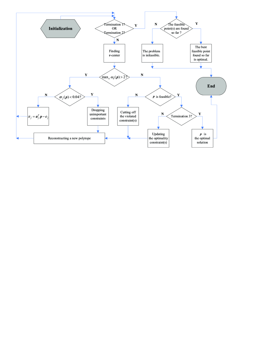
Figure 1: Flow chart of the LLBCP algorithm.

In Fig. 1 we give a detailed flow chart of the LLBCP algorithm; and in Algorithm 1, we give the step-by-step description of the algorithm. The key components of the LLBCP algorithm are then elaborated next.

Algorithm 1 : LLBCP Algorithm

1:Initialization

2:Set $\epsilon>0$, $\tau=\frac{1}{\epsilon}$, $i=0$;

3:According to (III-A), set $\mbox{\boldmath$A$}=[\mbox{\boldmath$I$}_{K}\;\;-\mbox{\boldmath$I$}_{K}\;\;\mbox{\boldmath$1$}_{K}]^{T}$, $\mbox{\boldmath$c$}=[-\frac{1}{\epsilon}\mbox{\boldmath$1$}_{K}^{T}\;\;-\frac{1}{\epsilon}\mbox{\boldmath$1$}_{K}^{T}\;\;-\frac{1}{\epsilon}\sqrt{K}]^{T}$, $\mbox{\boldmath$p$}=\mbox{\boldmath$0$}_{K}$, and $\mbox{\boldmath$s$}=\mbox{\boldmath$A$}\mbox{\boldmath$p$}-\mbox{\boldmath$c$}$;

4:Set $\pi_{k}=\frac{1}{\epsilon},k=1,...,2K,\pi_{2K+1}=\frac{1}{\epsilon}\sqrt{K};$

5:If necessary, find approximate $\tau$-center.

6:The Iterative step

7:if Termination 1: $N\geq 4093K\log_{2}(1/\epsilon)$                                                                                                                            or Termination 2: $\min_{k}({\mbox{\boldmath$a$}^{T}_{k}\mbox{\boldmath$p$}-c_{k}})<\;\;\;10^{-5}\epsilon^{3}/[2K^{1.5}\log_{2}(1/\epsilon)]$ then

8:     STOP: the best feasible point found so far is optimal. Otherwise, no feasible point is found.

9:else

10:     Find a new approximate $\tau$-center $\mbox{\boldmath$p$}=\mbox{\boldmath$p$}^{i}$;

11:     Calculate $\omega_{k}(\mbox{\boldmath$p$})=\frac{\mbox{\boldmath$a$}^{T}_{k}\mbox{\boldmath$p$}-c_{k}}{\pi_{k}},\forall k$.

12:     Set $\omega_{k}(\mbox{\boldmath$p$})=1$ if $k$ indexes the lowerbound constraint that get added in Subcase 2.2.

13:     If $\omega_{\tilde{j}}(\mbox{\boldmath$p$})>2$, calculate $\varpi_{\tilde{j}}(\mbox{\boldmath$p$})$ as in (21).

14:     if  $\max_{k}(\omega_{k}(\mbox{\boldmath$p$}))>2$ then

15:         Case 1 :

16:         if for some $\tilde{j}$, we have $\varpi_{\tilde{j}}(\mbox{\boldmath$p$})<0.04$ then

17:              Subcase 1.1:

18:              Drop the hyperplane $\mbox{\boldmath$a$}_{\tilde{j}}$;

19:              Find a new approximate $\tau$-center.

20:         else

21:              Subcase 1.2:

22:              Reset $\pi_{\tilde{j}}=\mbox{\boldmath$a$}^{T}_{\tilde{j}}\mbox{\boldmath$p$}-c_{\tilde{j}}$, where $\tilde{j}$ be an index such that $\omega_{\tilde{j}}(\mbox{\boldmath$p$})>2$.

23:         end if

24:     end if

25:     if  $\max_{k}(\omega_{k}(\mbox{\boldmath$p$}))\leq 2$ then

26:         Case 2 :

27:         if $p$ is not feasible in the problem (III-A) then

28:              Subcase 2.1:

29:              For $\tilde{k}\in\tilde{\mbox{\boldmath$K$}}$, generate hyperplane(s) as in (22).

30:              Set $\pi_{N+\tilde{k}}=(\frac{\mbox{\boldmath$\nabla$}_{\mathrm{drop}}^{i,\tilde{k}}}{\|\mbox{\boldmath$\nabla$}_{\mathrm{drop}}^{i,\tilde{k}}\|})^{T}\mbox{\boldmath$p$}^{i}-(\frac{\mbox{\boldmath$\nabla$}_{\mathrm{drop}}^{i,\tilde{k}}}{\|\mbox{\boldmath$\nabla$}_{\mathrm{drop}}^{i,\tilde{k}}\|})^{T}\mbox{\boldmath$p$}$.

31:              Set $N\leftarrow N+|\tilde{\mbox{\boldmath$K$}}|$.

32:              Find a new approximate $\tau$-center.

33:         else

34:              Subcase 2.2:

35:              if Termination 3: $1.25N\tau<\epsilon$ then

36:                  $\mbox{\boldmath$p$}_{i}$ is the optimal solution, and STOP.

37:              else

38:                  set the lower bound $l=\mbox{\boldmath$1$}_{K}^{T}\mbox{\boldmath$p$}-1.25N\tau$ on optimal objective function of (III-A).

39:                  Let $l_{prev}$ denote previous lower bound. If $l_{prev}<l$, replace $\mbox{\boldmath$1$}_{K}^{T}\mbox{\boldmath$p$}\geq l_{prev}$ by $\mbox{\boldmath$1$}_{K}^{T}\mbox{\boldmath$p$}\geq l$.

40:                  Set $\tau\leftarrow\theta\tau$, where $\theta\in(0.5,1)$.

41:                  Find a new approximate $\tau$-center.

42:              end if

43:         end if

44:     end if

45:end if

III-B1 Finding $\tau$-center

(Lines 5, 10, 19, 32, 41 in Algorithm 1)

In each iteration i, we need to generate a trial point inside the polytope $\mathcal{{P}}^{i}=\{\mbox{\boldmath$p$}\in\mathbb{R}^{K}:{\mbox{\boldmath$A$}^{i}\mbox{\boldmath$p$}\geq\mbox{\boldmath$c$}^{i}}\}$. Here, we will generate the so-called $\tau$-center of the polytope $\mathcal{{P}}^{i}$ as the trial point. First we need to define the so-called logarithmic barrier function

$$f(\mbox{\boldmath$p$},\tau)=\frac{\mbox{\boldmath$1$}_{K}^{T}\mbox{\boldmath$p$}}{\tau}-\sum_{n}\log(s_{n})$$ (20)

where $s_{n}=\mbox{\boldmath$a$}_{n}^{T}\mbox{\boldmath$p$}-c_{n}$, and $\mbox{\boldmath$a$}_{n}^{T}$ is the n-th row of $A$. $\tau>0$ is the barrier parameter. For a given value of $\tau^{i}$, $\mbox{\boldmath$p$}^{i}(\tau^{i})$ denotes the unique minimizer of this barrier function. We refer this unique point as the $\tau$-center. Notice that an approximate $\tau$-center is sufficient to serve as a trial point. An approximate $\tau$-center for the $(i+1)$-th iteration can be obtained from an approximate $\tau$-center for the $i$-th iteration by applying $\mathcal{O}(1)$ Newton steps[29].

III-B2 Dropping unimportant constraints

(Lines 14-20 in Algorithm 1)

The $j$-th constraint (i.e., hyperplane) is dropped only if its slack $\mbox{\boldmath$a$}_{j}^{T}\mbox{\boldmath$p$}-c_{j}$ has doubled since $\omega_{j}$ was last reset (Line 14 in Algorithm 1) and its variational quantity $\varpi_{j}$ is small (Line 16 in Algorithm 1).

The variational quantity $\varpi_{j}$ is defined as:

$$\varpi_{j}=\frac{\mbox{\boldmath$a$}_{j}^{T}(\nabla^{2}f(\mbox{\boldmath$p$},\tau))^{-1}\mbox{\boldmath$a$}_{j}}{s_{j}^{2}},\;\;j=1,...,N,$$ (21)

where $N$ denote the number of the rows of $A$. The variational quantities give an indication of the relative importance of the constraint $\mbox{\boldmath$a$}_{j}^{T}\mbox{\boldmath$p$}\geq c_{j}$.

If $k$ indexes the lower bound, $\omega_{k}(\mbox{\boldmath$p$})=1$ (Line 12 in Algorithm 1). Otherwise, $\omega_{k}(\mbox{\boldmath$p$})=\frac{\mbox{\boldmath$a$}^{T}_{k}\mbox{\boldmath$p$}-c_{k}}{\pi_{k}}$ (Line 11 in Algorithm 1), where $\pi_{k}$ is initialized as $\pi_{k}=\frac{1}{\epsilon},k=1,...,2K,\pi_{2K+1}=\frac{1}{\epsilon}\sqrt{K}$ (Line 4 in Algorithm 1), and is updated as $\pi_{k}=\mbox{\boldmath$a$}^{T}_{k}\mbox{\boldmath$p$}-c_{k}$ (Line 22 in Algorithm 1) if $\max_{k}(\omega_{k}(\mbox{\boldmath$p$}))>2$(Line 14 in Algorithm 1) and $\varpi_{k}(\mbox{\boldmath$p$})\geqslant 0.04$ (Line 16 in Algorithm 1).

III-B3 Checking feasibility

Given a trial point $\mbox{\boldmath$p$}^{i}\in\mathcal{{P}}^{i}$, we can verify its feasibility for problem (III-A) by checking if it satisfies the first constraint $\mathop{\inf}\limits_{{t_{k}}>\rho_{k}}{G_{k}}\left({{\mbox{\boldmath$p$}}^{i},{t_{k}}}\right)\leqslant 0,\forall k$. This requires solving a minimization problem over $t_{k}>\rho_{k}$. Due to the unimodality of ${G_{k}}\left({{\mbox{\boldmath$p$}}^{i},{t_{k}}}\right)$ in $t_{k}$, we can simply take a line search procedure to find the minimizer $t_{k}^{*}$.

III-B4 Cutting off the violated constraint(s)

(Lines 29-31 in Algorithm 1)

If the trial point $\mbox{\boldmath$p$}^{i}\in\mathcal{{P}}^{i}$ is infeasible, then a hyperplane is generated at $\mbox{\boldmath$p$}^{i}$ as follows:

$$\Big{(}\frac{\mbox{\boldmath$\nabla$}_{\mathrm{drop}}^{i,\tilde{k}}}{\|\mbox{\boldmath$\nabla$}_{\mathrm{drop}}^{i,\tilde{k}}\|}\Big{)}^{T}\mbox{\boldmath$p$}\leq\Big{(}\frac{\mbox{\boldmath$\nabla$}_{\mathrm{drop}}^{i,\tilde{k}}}{\|\mbox{\boldmath$\nabla$}_{\mathrm{drop}}^{i,\tilde{k}}\|}\Big{)}^{T}\mbox{\boldmath$p$}^{i},\;\;\;\tilde{k}\in\tilde{\mbox{\boldmath$K$}}$$ (22)

where $\tilde{\mbox{\boldmath$K$}}=\{k:{G_{k}}\left({{\mbox{\boldmath$p$}}^{i},{t_{k}^{*}}}\right)>0,\;k=1,...,K\}$, and $\mbox{\boldmath$\nabla$}_{\mathrm{drop}}^{i,\tilde{k}}$ is the gradient of ${G_{k}}\left({{\mbox{\boldmath$p$}},{t_{k}^{*}}}\right)$ with respect to $p$ at $\mbox{\boldmath$p$}^{i}$, with the k-th component given by

$$\nabla_{\mathrm{drop},k}^{i,\tilde{k}}=\frac{\partial{G_{\tilde{k}}\left({{\mbox{\boldmath$p$}},{t_{\tilde{k}}^{*}}}\right)}}{\partial{p_{k}}}|_{p_{k}={p_{k}^{i}}}$$ (23)

III-B5 Updating lower bound and reducing barrier parameter

(Lines 38-40 in Algorithm 1) If the point $\mbox{\boldmath$p$}^{i}$ is feasible but not optimal, the lower bound $l=\mbox{\boldmath$1$}_{K}^{T}\mbox{\boldmath$p$}-1.25N\tau$ to the optimal objective function value of problem (III-A) is updated (Lines 38-39 in Algorithm 1), and the value of the barrier parameter $\tau$ is reduced (Line 40 in Algorithm 1). Notice that according to the definition of (20), for a fixed value of $\tau>0$, it is desirable to minimize $f(\mbox{\boldmath$p$},\tau)$, leading to a balance between the objective function and centrality. When we need to drive the objective function value down, we just reduce the value of the barrier parameter $\tau$, leading to increasing emphasis on the objective function . When $\tau$ is driven to zero, we have the convergence to an optimal solution.

III-C Robust Max-Min SINR Optimization

We next consider the max-min SINR optimization problem in (II-B2). Since it is difficult to verify directly whether problem (II-B2) is convex, we use the similar method in [14] to solve (II-B2). Specifically, by introducing a slack variable $a>0$, the epigraph form of the robust max-min SINR optimization problem with individual power constraints (II-B2) is given by

$$\mathcal{S}({\mbox{\boldmath$p$}})\triangleq\left\{\begin{gathered}\mathop{\max}\limits_{\left\{{{p_{k}}}\right\}_{k=1}^{K},a}{\text{ }}a\hfill\\ {\rm s.t.}{\text{ }}\Pr\left({{\Gamma_{k}}\leqslant a}\right)\leqslant{\varepsilon_{k}},\ k=1,...,K\hfill\\ {\text{ }}0\leqslant{p_{k}}\leqslant{{\bar{p}}_{k}},\ k=1,...,K\hfill\\ \end{gathered}\right.$$ (24)

We demonstrate that solving $\mathcal{S}({\mbox{\boldmath$p$}})$ can be facilitated via solving a power optimization problem defined as

$$\mathcal{P}({\mbox{\boldmath$p$}},a)\triangleq\left\{\begin{gathered}\mathop{\min}\limits_{\left\{{{p_{k}}}\right\}_{k=1}^{K},b}{\text{ }}b\hfill\\ {\rm s.t.}{\text{ }}\Pr\left({{\Gamma_{k}}\leqslant a}\right)\leqslant{\varepsilon_{k}},\ k=1,...,K\hfill\\ {\text{ }}0\leqslant{p_{k}}\leqslant b{{\bar{p}}_{k}},\ k=1,...,K\hfill\\ \end{gathered}\right.$$ (25)

which can be solved using the similar method for solving the robust power minimization problem given in (II-B1). The connection between $\mathcal{S}({\mbox{\boldmath$p$}})$ and $\mathcal{P}({\mbox{\boldmath$p$}},a)$ is given by the following result, and the proof is given in Appendix B.

Proposition 2 $\mathcal{P}({\mbox{\boldmath$p$}},a)$ is strictly increasing and continuous in $a$ at any strictly feasible region and is related to $\mathcal{S}({\mbox{\boldmath$p$}})$ via $\mathcal{P}({\mbox{\boldmath$p$}},\mathcal{S}({\mbox{\boldmath$p$}}))=$1.

Since $\mathcal{P}({\mbox{\boldmath$p$}},a)$ is strictly increasing and continuous in $a$ at any strictly feasible region, there exists a unique $a^{*}$ satisfying $\mathcal{P}({\mbox{\boldmath$p$}},a^{*})$ = 1. It follows from Proposition 2 that solving $\mathcal{S}({\mbox{\boldmath$p$}})$ boils down to finding $a^{*}$ that satisfies $\mathcal{P}({\mbox{\boldmath$p$}},a)=1$. Due to monotonicity and continuity of $\mathcal{P}({\mbox{\boldmath$p$}},a)=1$, $a^{*}$ can be obtained by a simple bi-section search.

Finally we note that using the same approach, we can solve the problem of robust max-min SINR optimization problem with total power constraints given in (II-B2).

IV Robust Power Optimization for MISO Broadcast Channels

In this section, we treat a related power allocation problem for a MISO broadcast system with outage constraints on receiver MSE. Specifically, we consider the MSE-constrained power minimization problem in the downlink multiuser MISO system with Gaussian channel mismatch. We adopt the Bernstein approximation approach to convert the probablistic constraint into a deterministic convex constraint. Note that the similar problem has been considered in [17], where the Vysochanskii-Petunin inequality (VPI) is employed to obtain the conservative approximations to the probablistic constraints. We will demonstrate in Section IV the superiority of the Bernstein approach to the VPI method.

We consider a downlink multiuser MISO system with one base station (BS) equipped with $M$ antennas and $K$ single-antenna users. The BS transmits a symbol vector $\mbox{\boldmath$s$}=[s_{1},\ldots,s_{K}]^{T}\in\mathbb{C}^{K}$, where the symbol $s_{k}$ is intended for the $k$-th user. We denote the complete downlink channel as $\mbox{\boldmath$H$}\in\mathbb{C}^{K\times M}$. The BS is provided only with an estimate $\hat{\mbox{\boldmath$H$}}$ of $H$, where $\hat{\mbox{\boldmath$H$}}$ has full row rank. The CSI error matrix is given by $\mbox{\boldmath$\Delta$}=\mbox{\boldmath$H$}-\hat{\mbox{\boldmath$H$}}$, which is assumed to contain i.i.d. complex Gaussian entries, i.e.,

$$\delta_{k,j}\stackrel{{\scriptstyle\rm i.i.d.}}{{\sim}}{\cal N}_{c}(0,\sigma_{k,j}^{2}),k=1,...,K,j=1,...,M.$$ (26)

We assume that the beamforming matrix $\mbox{\boldmath$G$}\in\mathbb{C}^{M\times K}$ is set as the Moore-Penrose pseudoinverse of the available imperfect CSI, i.e., $\mbox{\boldmath$G$}=\hat{\mbox{\boldmath$H$}^{{\dagger}}}$. Our objective is to design the diagonal power allocation matrix $\mbox{\boldmath$Q$}^{1/2}=\mathrm{diag}(\sqrt{q_{1}},\ldots,\sqrt{q_{K}})$.

The $k$-th user equalizes its received signal using a one-tap equalizer with coefficient $q_{k}^{-1/2}$. Thus the symbol estimate at the equalizer output is given by

$$\hat{s}_{k}=q_{k}^{-1/2}\mbox{\boldmath$H$}[k,:]\mbox{\boldmath$G$}\mbox{\boldmath$Q$}^{1/2}\mbox{\boldmath$s$}+v_{k},\ \ \ k=1,\ldots,K$$ (27)

where $\mbox{\boldmath$H$}[k,:]$, denoting the $k$-th row of $H$, is the $k$-th user’s MISO channel; $v_{k}$ denotes the noise sample at the $k$-th user. We assume that $\mathbb{E}\{\mbox{\boldmath$ss$}^{H}\}=\mbox{\boldmath$I$}$, and $\mathbb{E}\{\mbox{\boldmath$vv$}^{H}\}=\mathrm{diag}(\eta_{1}^{2},\ldots,\eta_{K}^{2})$, where $\mbox{\boldmath$v$}=[v_{1},\ldots,v_{K}]^{T}$.

We use the mean-squared error (MSE) between the transmitted symbol and the receiver equalizer output as the QoS metric, i.e.,

$$\mathrm{MSE}_{k}=\mathbb{E}\{|s_{k}-\hat{s}_{k}|^{2}\},\ \ \ k=1,\ldots,K$$ (28)

We consider the following MSE-constrained power minimization problem. The objective is to minimize the total transmit power, subject to constraint that the probability of $\mathrm{MSE}_{k}$ being below a target value $\mu_{k}$ is no less than $\phi_{k}\in(0,1)$. That is,

$$\begin{gathered}\mathop{\min}\limits_{\mbox{\boldmath$Q$}\succeq{\bf 0}}\ \ \mathrm{tr}(\mbox{\boldmath$GQG$}^{H})\hfill\\ {\rm s.t.}\ \ \ \mathrm{Pr}\left(\mathrm{MSE}_{k}\leq\mu_{k}\right)\geq\phi_{k},\ k=1,...,K\hfill\\ \end{gathered}$$ (32)

Now using the Bernstein approximation we can convert (32) into a convex optimization problem, as stated in the following result. The proof is given in Appendix C.

Proposition 3 The following optimization problem (36) is a convex conservative approximation to the optimization problem in (32):

$$\begin{gathered}\mathop{\min}\limits_{\mbox{\boldmath$Q$}\succeq{\bf 0}}\ \ \mathrm{tr}(\mbox{\boldmath$GQG$}^{H})\hfill\\ {\rm s.t.}\ \ \ \mathop{\inf}\limits_{{t_{k}}>0}{G_{k}^{\mathrm{MSE}}}\left({\mbox{\boldmath$Q$},{t_{k}}}\right)\leqslant 0,\ k=1,...,K\hfill\\ \end{gathered}$$ (36)

where $G_{k}^{\mathrm{MSE}}\left({\mbox{\boldmath$Q$},{t}_{k}}\right)$ is defined in (37)

$$G_{k}^{\mathrm{MSE}}\left({\mbox{\boldmath$Q$},{t}_{k}}\right) \triangleq (\eta_{k}^{2}-q_{k}\mu_{k})-\frac{{t}_{k}}{2}\log\det\Big{(}\mbox{\boldmath$I$}-\frac{2}{{t}_{k}}\mathbf{\Lambda}_{k}\mbox{\boldmath$GQG$}^{H}\Big{)}-t_{k}\log(1-\phi_{k}),$$ (37)

with $\mbox{\boldmath$\Lambda$}_{k}\triangleq{\rm diag}(\sigma_{k,1}^{2},...,\sigma_{k,M}^{2})$.

We can solve problem (36) using the LLBCP algorithm discussed in Section III-B.

V Simulation Results

In this section, we present extensive simulation results to illustrate the performance of proposed Bernstein approximation approach to probability-constrained power optimization in wireless networks. First we illustrate the performance in MISO interference channels. Then we illustrate the performance in MISO broadcast channels and compare it with that of the VPI-based approach given in [17].

V-A SINR-constrained Power Minimization in MISO Interference Channels

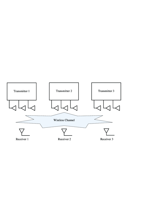
Figure 2: The simulated MISO interference channel.

We consider a MISO interference channel shown in Fig. 2, where the distance from a transmitter to the corresponding receiver is 200m, and the distance between the adjacent transmitters or receivers is 400m. The channel from the $j$-th transmitter to the $k$-th receiver is modeled as

$${\mbox{\boldmath$h$}}_{k,j}=\left(\frac{200}{d_{k,j}}\right)^{3.5}l_{k,j}\bar{\mbox{\boldmath$h$}}_{k,j}$$ (38)

where $d_{k,j}$ is the distance from the $j$-th transmitter to the $k$-th receiver; $10\log_{10}l_{k,j}\sim{\cal N}(0,8)$ is a real Gaussian random variable accounting for the large scale log-normal shadowing; $\bar{\mbox{\boldmath$h$}}_{k,j}\sim\mathcal{N}_{c}(\mbox{\boldmath$0$}_{M},\mbox{\boldmath$I$}_{M})$ is a circularly symmetric complex Gaussian random vector accounting for Rayleigh fast fading.

We define

$$\kappa_{k,j}^{m}\triangleq\frac{{\rm Var}({\hat{h}_{k,j}^{m}})}{{\rm Var}(\delta_{k,j}^{m})}\times 100\%$$ (39)

where ${\rm Var}({\hat{h}_{k,j}^{m}})$ and ${\rm Var}(\delta_{k,j}^{m})$ are the standard deviations of the channel ${h}_{k,j}^{m}$ and the channel error $\delta_{k,j}^{m}$, respectively. For simplicity, we assume $\kappa_{k,j}^{m}=\kappa,\forall k,j,m$, and consider cases of $\kappa\in\{1\%,5\%,10\%,15\%\}$ in the following simulations. Moreover, we assume that all receivers have the same SINR level $\alpha$.

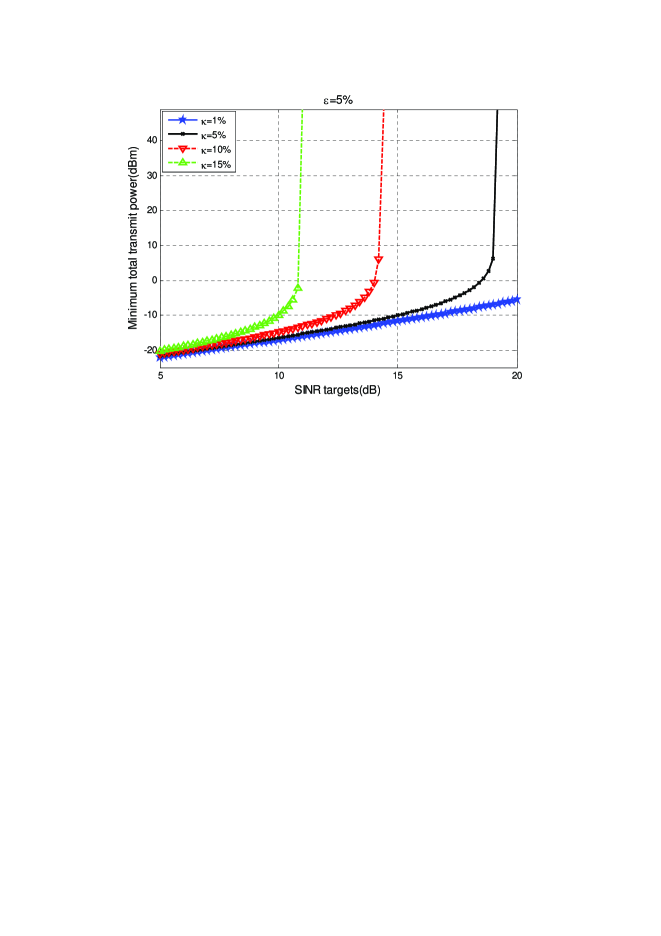
Figure 3: Minimum total transmit power versus SINR level $\alpha$, for different values of $\kappa$ and for $\varepsilon=5\%$ in a MISO interference channel.

We consider the SINR-constrained power minimization problem in MISO interference channels, given by (II-B1). We solve this problem by using the Bernstein approximation and the LLBCP algorithm, as discussed in Section III.A-B. First we consider the impact of channel error variance on the power control performance. Fig. 3 shows the minimum total transmit power, $P_{T}^{\min}(\alpha)=\sum_{k}p_{k}(\alpha)$ versus the required SINR level $\alpha$ for the fixed outage probability $\varepsilon=5\%$ and for the different channel uncertainty levels $\kappa$. It is seen that when the channel uncertainty increases, it takes more power to meet the SINR outage requirement. For a fixed channel uncertainty level $\kappa$, as the target SINR value $\alpha$ increases, it becomes exceedingly difficult to meet the outage requirement; and moreover, the transmit power increases drastically near some limiting SINR value. This limiting value is the one which makes the optimization problem infeasible. Therefore the effect of imperfect CSI is more difficult to cope with when target SINR is high. As the channel uncertainty increases, the maximum feasible SINR value $\alpha$ also decreases.

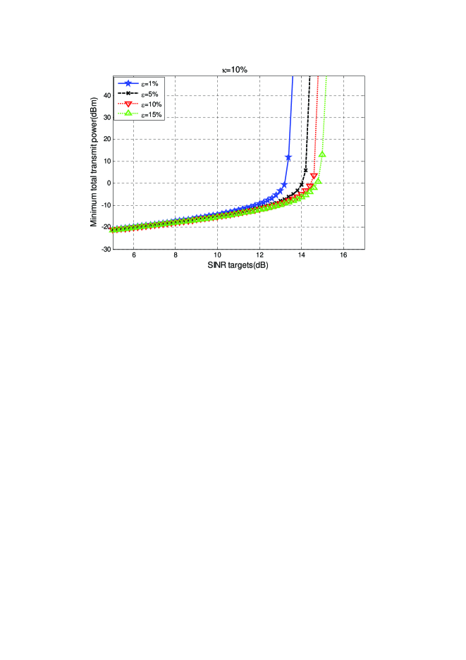
Figure 4: Minimum total transmit power versus SINR level $\alpha$, for different values of $\varepsilon$ and for $\kappa=10\%$ in a MISO interference channel.

We next consider the impact of the outage probability requirement on the power control performance. Fig. 4 illustrates $P_{T}^{\min}(\alpha)$ versus the target SINR level $\alpha$ for the fixed channel uncertainty $\kappa=10\%$ and for different outage probability values $\varepsilon$. It is seen that as the outage requirement becomes more stringent, i.e., when $\varepsilon$ becomes smaller, it takes more power to meet the SINR outage requirement, and the maximum feasible SINR value $\alpha$ becomes smaller.

V-B Max-Min SINR Optimization in MISO Interference Channels

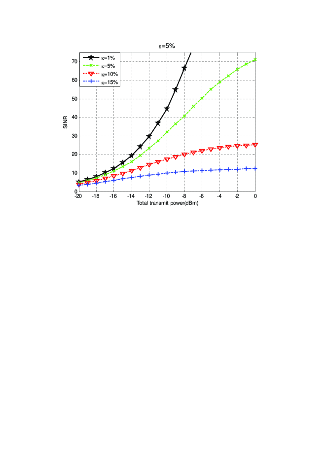
Figure 5: Maximum achievable SINR versus maximum allowable total transmit power, for different values of $\kappa$ and for $\varepsilon=5\%$, in a MISO interference channel.

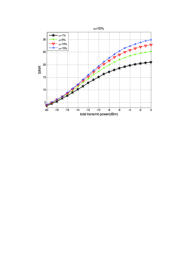
Figure 6: Maximum achievable SINR versus maximum allowable total transmit power, for different values of $\varepsilon$ and for $\kappa=10\%$, in a MISO interference channel.

We now consider the max-min SINR optimization problems in MISO interference channels under either individual or total transmit power constraint, given by (II-B2)-(II-B2). Again the Berinstein approximation and the LLBCP algorithm are employed to solve the problems, as outlined in Section III.C. In Fig. 5, we plot the maximum achievable SINR versus the maximum allowable total transmit power for fixed outage probability $\varepsilon=5\%$ and for different values of the mismatched error variance $\kappa$. In Fig. 6, we plot the maximum achievable SINR versus the maximum allowable total transmit power for fixed $\kappa=10\%$ and for different $\varepsilon$. It is seen that for a given maximum allowable total transmit power, the maximum achievable SINR decreases as the channel uncertainty $\kappa$ increases, or as the outage probability $\varepsilon$ decreases.

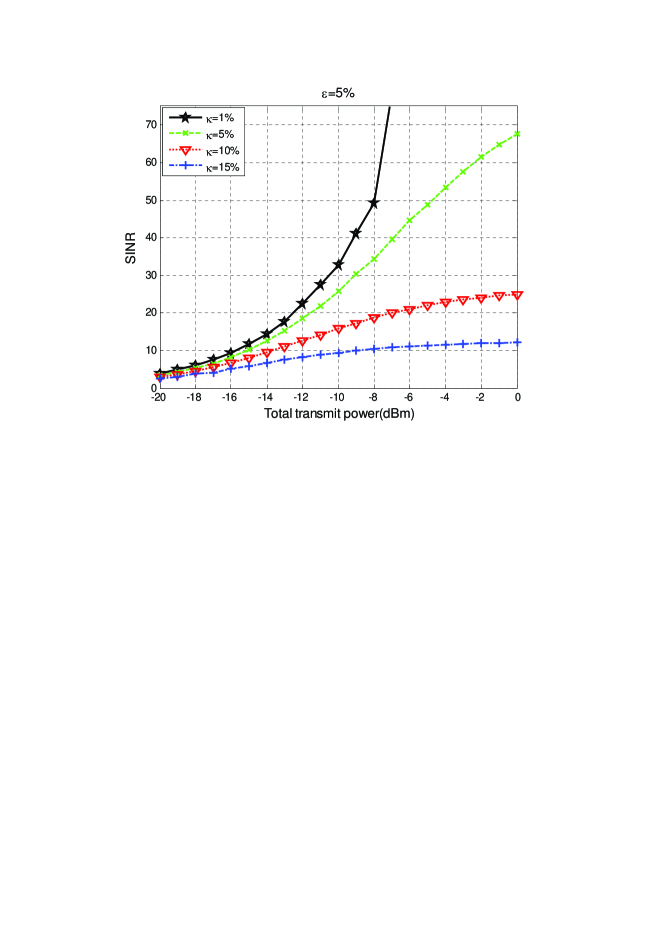
Figure 7: Maximum achievable SINR versus maximum allowable total transmit power, under individual power constraints, for different values of $\kappa$ and for $\varepsilon=5\%$, in a MISO interference channel.

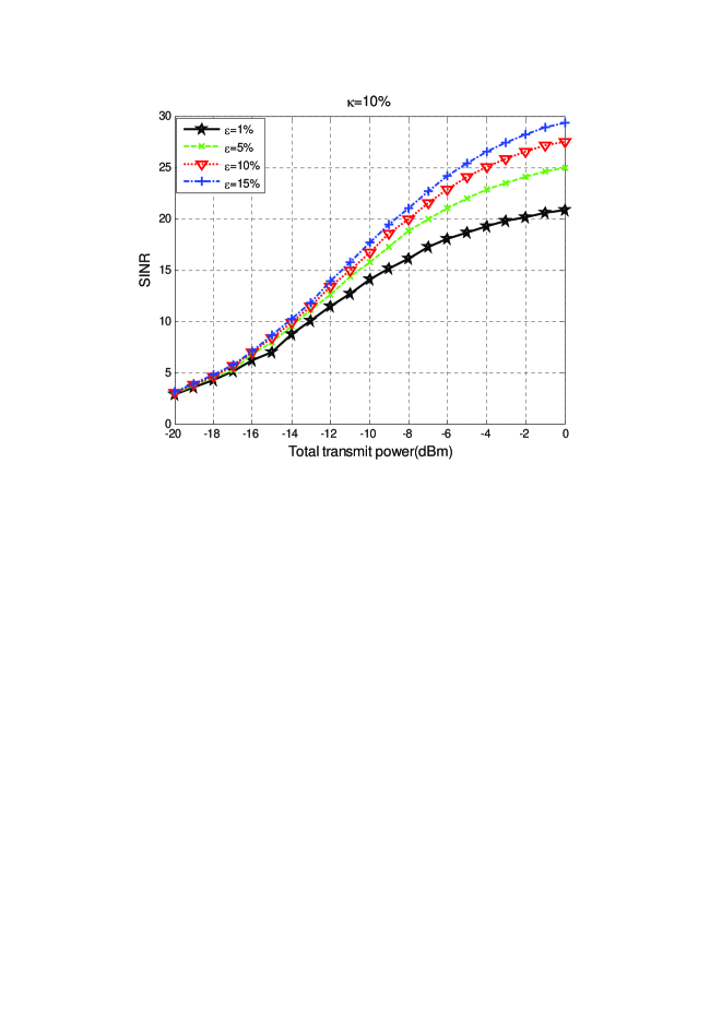
Figure 8: Maximum achievable SINR versus maximum allowable total transmit power, under individual power constraints, for different values of $\varepsilon$ and for $\kappa=10\%$, in a MISO interference channel.

Next we consider the case where the individual transmit powers are constrained. We assume that the transmitters have the same maximum allowable individual transmit power $\bar{p}_{k}=\bar{p}_{total}/K$, where $\bar{p}_{total}$ denotes the total transmit power. Fig. 7 shows the maximum achievable SINR versus the total transmit power, for fixed $\varepsilon=5\%$ and for different values of $\kappa$. Fig. 8 illustrates the maximum achievable SINRs versus the total transmit power, for fixed $\kappa=10\%$ and for different outage probability $\varepsilon$. It is seen that the maximum achievable SINR under the individual transmit power constraint suffers an SINR loss as compared to that under the total transmit power constraint.

V-C MSE-constrained Power Minimization in MISO Broadcast Channels

In this section, we illustrate the performance of the proposed Bernstein approximation approach to the MSE-constrained power minimization in a downlink MISO system, as discussed in Section IV, with comparison with the VPI-based approach proposed in [17].

We consider a downlink MISO system with $K=3$ users and the basestation is equipped with $M=3$ transmit antennas. We set a same MSE target for all users and choose $\mu_{1}=\mu_{2}=\mu_{3}=\mu$ from -15dB to -5dB. The channel coefficients are generated as i.i.d. complex Gaussian random variables with zero mean and unit variance. The channel error matrix is set as $\mbox{\boldmath$\Delta$}[k,:]=\sigma_{k}\mbox{\boldmath$\overline{\Delta}$}[k,:],k=1,...,K$, where $\mbox{\boldmath$\overline{\Delta}$}[k,:]\sim{\cal N}_{c}(\mbox{\boldmath$0$}_{M},\mbox{\boldmath$I$}_{M})$.

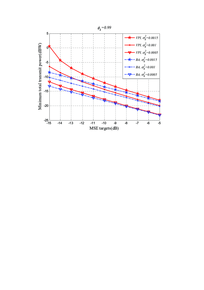
Figure 9: Minimum total transmit power versus the target MSE, for different values of $\sigma_{k}^{2}$ and for $\phi=0.99$, in a MISO broadcast channel.

First, we compare the total transmit power of the Bernstein approximation approach and that of the VPI-based method. In Fig. 9, the minimum total transmit power against the target MSE is plotted, for three channel error values $\sigma_{k}^{2}$=$1.5\times 10^{-3}$, $\sigma_{k}^{2}$=$10^{-3}$ and $\sigma_{k}^{2}$=$0.5\times 10^{-3}$, at the probabilistic guarantee $\phi_{k}=0.99$. It is seen that the proposed Bernstein approximation approach outperforms the VPI-based method in that it achieves lower total transmit power in all cases. Additional simulations show that the Bernstein approximation approach significantly outperforms the VPI-based method when the channel uncertainly is high (i.e., larger $\sigma_{k}^{2}$), and/or the targe MSE is low (i.e., small $\mu_{k}$), and/or the probabilistic guarantee is stringent (i.e., high $\phi_{k}$). For instance, we can see from Fig. 9 that for $\sigma_{k}^{2}$=$1.5\times 10^{-3}$, $\mu=$-15dB, and $\phi_{k}$=0.99, the transmit power difference between the two approaches is about 7dBW.

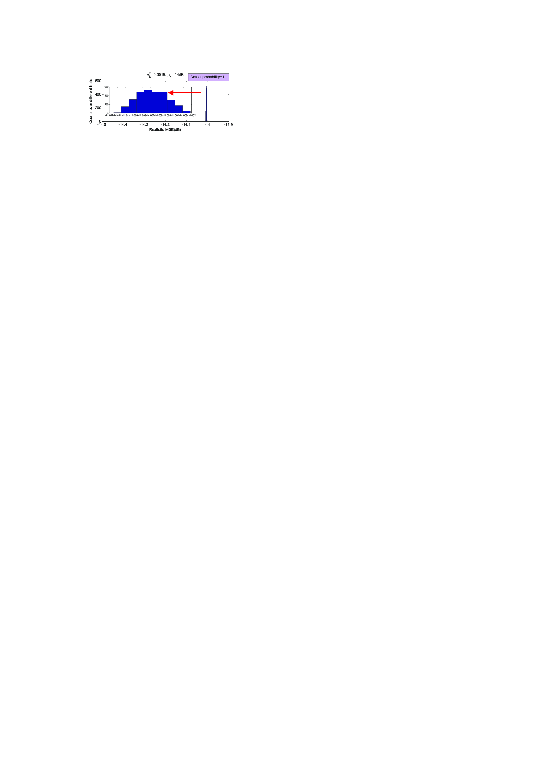
(a) Bernstein approximation approach

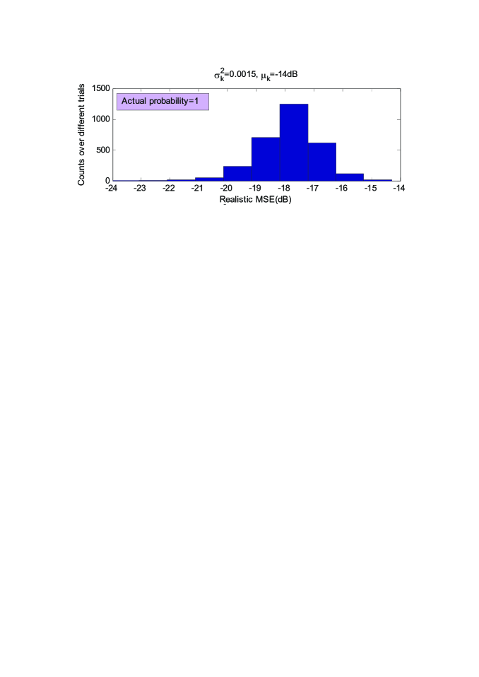
(b) VPI based approach

Figure 10: Histograms of the MSE under the Bernstein approximation approach and the VPI-based method. $\mu_{k}=-14$dB, and $\phi_{k}=0.99.$

In order to get more insight into the behavior of these two approaches, we verify the actual probabilistic guarantees by plotting the histograms of the MSE in Fig. 10(a)-10(b). The system parameters are $\sigma_{k}^{2}=1.5\times 10^{-3}$, $\mu_{k}=-14$dB, and $\phi_{k}=0.99.$ The results show that under both approaches, the probabilistic constraints are met. In fact, the actual probability is larger than the target probability, corroborating that both approaches provide conservative approximations to the original probabilistic constraints. However, it is seen that the histogram of the VPI-based method is much more spread than that of the Bernstein approximation approach. In particular, the MSE realizations under the Bernstein approximation approach concentrate sharply around the target MSE value $\mu$, whereas the MSE realizations under the VPI-based approach spread around an MSE value that is much lower than the target value $\mu$. Hence the VPI-based method provides a more conservative approximation to the original probabilistic constraint, and thus needs more transmit power to meet the resulting more stringent MSE constraint than the actual target constraint.

VI Conclusions

We have treated the problems of robust power allocation in multiuser MISO systems with imperfect transmitter-side CSI. The multi-antenna transmitters are assumed to employ some fixed beamformers to transmit data and the transmit powers need to be optimized to satisfy certain QoS constraints, taking into account the uncertainty in the available CSI. Specifically, for MISO interference channels, we have considered the transmit power minimization problem and the max-min SINR problem, subject to the constraints on the SINR outage probabilities. For MISO broadcast channels, we have considered the transmit power minimization problem subject to the constraints on the MSE outage probabilities. Our key contribution is to employ the Bernstein approximation to conservatively transform the probabilistic constraints into deterministic ones, and consequently convert the original stochastic optimization problems into convex optimization problems. We have provided extensive simulation results to demonstrate the effectiveness of the proposed robust power optimization techniques.

Appendix

VI-A Proof of Proposition 1

Proof: We have

$${\Gamma_{k}}=\frac{{{p_{k}}{{\left|{{\mbox{\boldmath$h$}_{kk}^{H}}{\mbox{\boldmath$g$}_{k}}}\right|}^{2}}}}{{\eta_{k}^{2}+\sum\limits_{j\neq k}{{p_{j}}{{\left|{{\mbox{\boldmath$h$}_{kj}^{H}}{\mbox{\boldmath$g$}_{j}}}\right|}^{2}}}}}\leqslant{\alpha_{k}}$$ (40)

$$\Longleftrightarrow{\alpha_{k}}\eta_{k}^{2}+{\alpha_{k}}\sum\limits_{j\neq k}{{p_{j}}{{\left|{{\mbox{\boldmath$h$}_{kj}^{H}}{\mbox{\boldmath$g$}_{j}}}\right|}^{2}}}-{p_{k}}{\left|{{\mbox{\boldmath$h$}_{kk}^{H}}{\mbox{\boldmath$g$}_{k}}}\right|^{2}}\geqslant 0$$ (41)

Plugging (2) into (41), we obtain (42),

$${F_{k}}\left({{\mbox{\boldmath$p$}},{{\mbox{\boldmath$\xi$}}_{k}}}\right) \triangleq {{\alpha_{k}}\eta_{k}^{2}+{\alpha_{k}}\sum\limits_{j\neq k}{{{p_{j}}\underbrace{{{\left|{\mbox{\boldmath$\hat{h}$}_{kj}^{H}\mbox{\boldmath$g$}_{j}+\mbox{\boldmath$\delta$}_{kj}^{H}\mbox{\boldmath$g$}_{j}}\right|}^{2}}}_{{\xi}_{kj}}}}}-{{p_{k}}\underbrace{{{\left|{\mbox{\boldmath$\hat{h}$}_{kk}^{H}\textbf{g}_{k}+\mbox{\boldmath$\delta$}_{kk}^{H}\mbox{\boldmath$g$}_{k}}\right|}^{2}}}_{{\xi}_{kk}}}$$ (42)

$$= {{\alpha_{k}}\eta_{k}^{2}+{\alpha_{k}}\sum\limits_{j\neq k}{{{p_{j}}{{\xi}_{kj}}}}}-{{p_{k}}{{\xi}_{kk}}}\geqslant 0$$

where ${\bm{\xi}_{k}}\triangleq\left[{{\xi_{k1}},{\xi_{k2}},...,{\xi_{kK}}}\right]^{T}$. Note that ${F_{k}}\left({{\mbox{\boldmath$p$}},{{\mbox{\boldmath$\xi$}}_{k}}}\right)$ in (42) is in the form of (10).

Since $\mbox{\boldmath$\delta$}_{kj},\forall j$ are independent, $\xi_{kj},\forall j$ are independent random variables. Furthermore, from (3), it follows that $\mbox{\boldmath$\delta$}_{kj}^{H}\mbox{\boldmath$g$}_{j}+\mbox{\boldmath$\hat{h}$}_{kj}^{H}\mbox{\boldmath$g$}_{j}\stackrel{{\scriptstyle\mbox{\small{i.i.d.}}}}{{\sim}}\mathcal{N}_{c}\left({\mbox{\boldmath$\hat{h}$}_{kj}^{H}\mbox{\boldmath$g$}_{j},\sigma^{2}_{kj}{{\left|{\bm{1}^{T}\mbox{\boldmath$g$}_{j}}\right|}^{2}}}\right)$. Then by normalizing $\xi_{kj}$ by the variance $\frac{\sigma^{2}_{kj}}{2}\left|{\bm{1}^{T}\mbox{\boldmath$g$}_{j}}\right|^{2}$ of the real or imaginary component, we obtain the following noncentral $\chi^{2}$ random variable with two degrees of freedom

$$\frac{\xi_{kj}}{\frac{\sigma^{2}_{kj}}{2}\left|{\bm{1}^{T}\mbox{\boldmath$g$}_{j}}\right|^{2}} \sim \chi_{2}^{2}\Big{(}\frac{|\mbox{\boldmath$\hat{h}$}_{kj}^{H}\mbox{\boldmath$g$}_{j}|^{2}}{\frac{\sigma^{2}_{kj}}{2}|{\bm{1}^{T}\mbox{\boldmath$g$}_{j}}|^{2}}\Big{)}.$$ (43)

Thus can write the logarithm of the moment generating function of ${F_{k}}\left({{\mbox{\boldmath$p$}},{\bm{\xi}_{k}}}\right)$ as (44)

$$\log\mathbb{E}\left[{\exp\left({{t_{k}^{-1}}{F_{k}}\left({{\mbox{\boldmath$p$}},{\bm{\xi}_{k}}}\right)}\right)}\right]=\log{\mathbb{E}}\left[{\exp\left({t_{k}^{-1}}{\alpha_{k}}\eta_{k}^{2}+{t_{k}^{-1}}{\alpha_{k}}\sum\limits_{j\neq k}{{{p_{j}}\xi_{kj}}}-{{t_{k}^{-1}}{p_{k}}\xi_{kk}}\right)}\right]$$ (44)

$$= {{t_{k}^{-1}}{\alpha_{k}}\eta_{k}^{2}}+\sum\limits_{j\neq k}\log{\mathbb{E}}\Big{\{}\exp\Big{[}\underbrace{\Big{(}\frac{\sigma^{2}_{kj}}{2}|{\bm{1}^{T}\mbox{\boldmath$g$}_{j}}|^{2}t_{k}^{-1}\alpha_{k}p_{j}\Big{)}}_{t}\underbrace{\Big{(}\frac{\xi_{kj}}{\frac{\sigma_{kj}^{2}}{2}{|{\bm{1}^{T}\mbox{\boldmath$g$}_{j}}|}^{2}}\Big{)}}_{X}\Big{]}\Big{\}}$$

$$+\log{\mathbb{E}}\Big{\{}\exp\Big{[}{-\Big{(}\frac{\sigma^{2}_{kk}}{2}|{\bm{1}^{T}\mbox{\boldmath$g$}_{k}}|^{2}t_{k}^{-1}p_{k}\Big{)}}{\Big{(}\frac{\xi_{kk}}{\frac{\sigma_{kk}^{2}}{2}{|{\bm{1}^{T}\mbox{\boldmath$g$}_{k}}|}^{2}}\Big{)}}\Big{]}\Big{\}}$$

$$= {{t_{k}^{-1}}{\alpha_{k}}\eta_{k}^{2}}+\sum\limits_{j\neq k}{{\left[{\frac{{t_{k}^{-1}{\alpha_{k}}{p_{j}}{{\left|{\mbox{\boldmath$\hat{h}$}_{kj}^{H}\mbox{\boldmath$g$}_{j}}\right|}^{2}}}}{{1-t_{k}^{-1}{\alpha_{k}}{p_{j}}{\sigma_{kj}^{2}}{{\left|{\bm{1}^{T}\mbox{\boldmath$g$}_{j}}\right|}^{2}}}}-\log\left({1-t_{k}^{-1}{\alpha_{k}}{p_{j}}\sigma_{kj}^{2}{{\left|{\bm{1}^{T}\mbox{\boldmath$g$}_{j}}\right|}^{2}}}\right)}\right]}}$$

$$-{{\frac{{{t_{k}^{-1}p_{k}}{{\left|{\mbox{\boldmath$\hat{h}$}_{kk}^{H}\mbox{\boldmath$g$}_{k}}\right|}^{2}}}}{{1+t_{k}^{-1}{p_{k}}\sigma_{kk}^{2}{{\left|{\bm{1}^{T}\mbox{\boldmath$g$}_{k}}\right|}^{2}}}}-\log\left({1+t_{k}^{-1}{p_{k}}\sigma_{kk}^{2}{{\left|{\bm{1}^{T}\mbox{\boldmath$g$}_{k}}\right|}^{2}}}\right)}}$$

where (44) follows from the fact that for $X\sim\chi_{2}^{2}\left(\lambda\right)$, we have

$${\mathbb{E}}\left\{{\exp\left({tX}\right)}\right\}=\frac{{\exp\left({\frac{{\lambda t}}{{1-2t}}}\right)}}{\left({1-2t}\right)},\ \ \ {\rm with}\ \ t<\frac{1}{2}.$$ (45)

Now using (9), we obtain the Bernstein approximation (46) to the probabilistic constraint $\Pr\left({{\Gamma_{k}}\leqslant\alpha_{k}}\right)\leqslant{\varepsilon_{k}}$ in (II-B2).

$${\inf}_{{t_{k}}>\rho_{k}}{G_{k}}\left({{\mbox{\boldmath$p$}},{t_{k}}}\right)\triangleq t_{k}\log\mathbb{E}\left[{\exp\left({{t_{k}^{-1}}{F_{k}}\left({{\mbox{\boldmath$p$}},{\bm{\xi}_{k}}}\right)}\right)}\right]-t_{k}\log\varepsilon_{k}\ \leqslant 0.$$ (46)

Substituting (44) into (46), we obtain (III-A). Note that in order to meet the condition $t<\frac{1}{2}$ in (45), we should have

$$\;\;\frac{\sigma^{2}_{kj}}{2}|{\bm{1}^{T}\mbox{\boldmath$g$}_{j}}|^{2}t_{k}^{-1}\alpha_{k}p_{j} < \frac{1}{2},\ \ \ j\neq k$$ (47)

Hence we have

$$t_{k}>\alpha_{k}\max_{j\neq k}\{\sigma^{2}_{kj}p_{j}|{\bm{1}^{T}\mbox{\boldmath$g$}_{j}}|^{2}\}\triangleq\rho_{k}.$$ (48)

$\Box$

VI-B Proof of Proposition 2

The proof follows the similar line as that in [14]. Let us denote the set of powers obtained from solving $\mathcal{S}({\mbox{\boldmath$\bar{p}$}})$ by $\left\{{p_{k}^{*}}\right\}$ and their corresponding minimal SINR by $\alpha_{k}^{*}$. From the definition of $S({\mbox{\boldmath$\bar{p}$}})$ we have ${p_{k}}\leqslant{\bar{p}_{k}},\forall k$ and $\mathop{\min}\limits_{k}\left\{{\alpha_{k}^{*}}\right\}=\mathcal{S}({\mbox{\boldmath$\bar{p}$}})\Rightarrow\alpha_{k}^{*}\geqslant\mathcal{S}({\mbox{\boldmath$\bar{p}$}}),\forall k$. As a result from the definition of $\mathcal{P}({\mbox{\boldmath$\bar{p}$}},a)$ we find that for the choice of $\left\{{p_{k}^{*}}\right\}$, the choice of $b=1$ is achievable for $\mathcal{P}({\mbox{\boldmath$\bar{p}$}},\mathcal{S}({\mbox{\boldmath$\bar{p}$}}))$ and therefore $\mathcal{P}({\mbox{\boldmath$\bar{p}$}},\mathcal{S}({\mbox{\boldmath$\bar{p}$}}))\leqslant 1$.

Next we show that $\mathcal{P}({\mbox{\boldmath$\bar{p}$}},\mathcal{S}({\mbox{\boldmath$\bar{p}$}}))$ cannot be less than one. Let us denote the set of powers obtained by solving $\mathcal{P}({\mbox{\boldmath$\bar{p}$}},\mathcal{S}({\mbox{\boldmath$\bar{p}$}}))$ by $\left\{{p_{k}^{**}}\right\}$. From the definition of $\mathcal{P}({\mbox{\boldmath$\bar{p}$}},\mathcal{S}({\mbox{\boldmath$\bar{p}$}}))$ we clearly have $\alpha_{k}^{**}\geqslant\mathcal{S}({\mbox{\boldmath$\bar{p}$}}),\forall k$. If $\mathcal{P}({\mbox{\boldmath$\bar{p}$}},\mathcal{S}({\mbox{\boldmath$\bar{p}$}}))<1$, i.e., if $\mathop{\max}\limits_{k}\frac{{p_{k}^{**}}}{{{{\bar{p}}_{k}}}}=c<1$, then we define the set of powers $\left\{{{{\hat{p}}_{k}}}\right\}=\left\{{{{p_{k}^{**}}\mathord{\left/{\vphantom{{p_{k}^{**}}c}}\right.\kern-1.2pt}c}}\right\}$. $\left\{{{{\hat{p}}_{k}}}\right\}$ clearly satisfy the power constraints and we have their corresponding SINRs satisfying

$$\begin{array}[]{l}\hat{\Gamma}_{k}=\frac{{\hat{p}_{k}\left|{\mbox{\boldmath$h$}_{kk}\mbox{\boldmath$g$}_{k}}\right|^{2}}}{{\sigma_{k}^{2}+\sum\limits_{j\neq k}{\hat{p}_{j}\left|{\mbox{\boldmath$h$}_{kj}\mbox{\boldmath$g$}_{j}}\right|^{2}}}}=\frac{{\frac{{p_{k}^{**}}}{c}\left|{\mbox{\boldmath$h$}_{kk}\mbox{\boldmath$g$}_{k}}\right|^{2}}}{{\sigma_{k}^{2}+\sum\limits_{j\neq k}{\frac{{p_{j}^{**}}}{c}\left|{\mbox{\boldmath$h$}_{kj}\mbox{\boldmath$g$}_{j}}\right|^{2}}}}\\ \;\;\;\;\;=\frac{{p_{k}^{**}\left|{\mbox{\boldmath$h$}_{kk}\mbox{\boldmath$g$}_{k}}\right|^{2}}}{{c\sigma_{k}^{2}+\sum\limits_{j\neq k}{p_{j}^{**}\left|{\mbox{\boldmath$h$}_{kj}\mbox{\boldmath$g$}_{j}}\right|^{2}}}}>\frac{{p_{k}^{**}\left|{\mbox{\boldmath$h$}_{kk}\mbox{\boldmath$g$}_{k}}\right|^{2}}}{{\sigma_{k}^{2}+\sum\limits_{j\neq k}{p_{j}^{**}\left|{\mbox{\boldmath$h$}_{kj}\mbox{\boldmath$g$}_{j}}\right|^{2}}}}\\ \end{array}$$

Since $c<1$, ${\hat{\Gamma}_{k}}>\Gamma_{k}^{**}$. Therefore, we have found a set of powers which satisfy the power constraints and yet yield a strictly larger minimal SINR compared to what the powers $\left\{{p_{k}^{**}}\right\}$ obtain. This contradicts the optimality of $\left\{{p_{k}^{**}}\right\}$ and therefore $\mathcal{P}({\mbox{\boldmath$\bar{p}$}},\mathcal{S}({\mbox{\boldmath$\bar{p}$}}))=1$. The strict monotonicity and continuity of $\mathcal{P}({\mbox{\boldmath$\bar{p}$}},a)$ in $a$, at any strictly feasible region, follows from a similar line of argument. $\Box$

VI-C Proof of Proposition 3

Proof: To be consistent with (7), we rewrite the constraint $\mathrm{Pr}\left(\mathrm{MSE}_{k}\leq\mu_{k}\right)\geq\phi_{k}$ as $\mathrm{Pr}\left(\mathrm{MSE}_{k}\geq\mu_{k}\right)\leq 1-\phi_{k}.$ Using (27) and (28) we have

$$\mathrm{MSE}_{k}=q_{k}^{-1}\mbox{\boldmath$\Delta$}[k,:]\mbox{\boldmath$GQG$}^{H}\mbox{\boldmath$\Delta$}[k,:]^{H}+q_{k}^{-1}\eta_{k}^{2}.$$ (49)

Thus the condition $\mathrm{MSE}_{k}\geq\mu_{k}$ becomes

$$F_{k}(\mbox{\boldmath$Q$},\mbox{\boldmath$\Delta$}[k,:])\triangleq\mbox{\boldmath$\Delta$}[k,:]\mbox{\boldmath$GQG$}^{H}\mbox{\boldmath$\Delta$}[k,:]^{H}+\eta_{k}^{2}-q_{k}\mu_{k}\geq 0.$$ (50)

Note that $\mbox{\boldmath$\Delta$}[k,:]$ is a zero-mean complex Gaussian random vector with a diagonal covariance matrix $\mbox{\boldmath$\Lambda$}_{k}\triangleq{\rm diag}(\sigma_{k,1}^{2},...,\sigma_{k,M}^{2})$. Thus we have (51) [30].

$$\mathbb{E}\Big{\{}\exp\Big{(}t_{k}^{-1}\mbox{\boldmath$\Delta$}[k,:]\mbox{\boldmath$GQG$}^{H}\mbox{\boldmath$\Delta$}[k,:]^{H}\Big{)}\Big{\}}=\frac{1}{\sqrt{\det(\mbox{\boldmath$I$}-\frac{2}{{t}_{k}}\mbox{\boldmath$\Lambda$}_{k}\mbox{\boldmath$GQG$}^{H})}}.$$ (51)

Then the Bernstein approximation to the probabilistic constraint $\mathrm{Pr}\left(\mathrm{MSE}_{k}\geq\mu_{k}\right)\leq 1-\phi_{k}$ becomes $\inf_{t_{k}>0}G_{k}^{\mathrm{MSE}}\left({\mbox{\boldmath$Q$},{t}_{k}}\right)\leq 0$, where $G_{k}^{\mathrm{MSE}}\left({\mbox{\boldmath$Q$},{t}_{k}}\right)$ is defined in (52)

$$G_{k}^{\mathrm{MSE}}\left({\mbox{\boldmath$Q$},{t}_{k}}\right) \triangleq t_{k}\log\mathbb{E}\left[{\exp\left({{t_{k}^{-1}}{F_{k}}\left({\mbox{\boldmath$Q$}},{\bm{\Delta}}[k,:]\right)}\right)}\right]-t_{k}\log(1-\phi_{k})$$ (52)

$$= (\eta_{k}^{2}-q_{k}\mu_{k})-\frac{{t}_{k}}{2}\log\det\Big{(}\mbox{\boldmath$I$}-\frac{2}{{t}_{k}}\mathbf{\Lambda}_{k}\mbox{\boldmath$GQG$}^{H}\Big{)}-t_{k}\log(1-\phi_{k}).$$

$\Box$

References

• [1] S. Shafiee and S. Ulukus, โ€œAchievable rates in Gaussian MISO channels with secrecy constraints,โ€ in Proc. IEEE ISIT, 2007, pp.2466-2470, Nice, France, June 2007.
• [2] E.A. Jorswieck, E.G. Larsson, and D. Danev, โ€œComplete characteriza- tion of the Pareto boundary for the MISO interference channel,โ€IEEE Trans. Sig. Proc., 56(10):5292-5296, Oct. 2008.
• [3] M.T. Ivrlac and J.A. Nossek. โ€œIntercell-interference in the Gaussian MISO broadcast channel,โ€ in Proc. IEEE GLOBECOM, 2007, pp.3195-3199, Washington D.C., Nov. 2007.
• [4] M. Castaneda, A. Mezghani, and J.A. Nossek, โ€œOn maximizing the sum network MISO broadcast capacity,โ€ in Proc. Intโ€™l ITG Workshop on Smart Antennas (WSAโ€™08), pp. 254-261, Vienna, Austria, Feb. 2008.
• [5] B. Song, Y.-H. Lin, and R.L. Cruz, โ€œ Weighted max-min fair beamforming, power control, and scheduling for a MISO downlink,โ€ IEEE Trans. Wireless Commun., 7(2):464-469, Feb. 2008.
• [6] E.G. Larsson and E.A. Jorswieck, โ€œCompetition versus cooperation on the MISO interference channel,โ€ IEEE J. Select. Areas Commun., 26(7):1059-1069, 2008.
• [7] M. Nokleby and A.L. Swindlehurst, โ€œBargaining and the MISO interference channel,โ€ EURASIP J. Advances Sig. Proc., vol. ID 368547, 13 pages, 2009.
• [8] N. Jindal, โ€œMIMO broadcast channels with finite-rate feedback,โ€ IEEE Trans. Inform. Theory, 52(11):5045-5060, Nov 2006.
• [9] A.B. Gershman, N.D. Sidiropoulos, S. Shahbazpanahi, M. Bengtsson, and B. Ottersten, โ€œConvex optimization-based beamforming: From receive to transmit and network designs,โ€ IEEE Sig. Proc. Mag., 27(3):62-75, May 2010.
• [10] M. Payaro, A. Pascual-Iserte, M.A. Lagunas, โ€œRobust power allocation designs for multiuser and multiantenna downlink communication systems through convex optimization,โ€ IEEE J. Select. Areas Commun., 25(7):1390-1401, 2007.
• [11] M.B. Shenouda and T.N. Davidson, โ€œConvex conic formulations of robust downlink precoder designs with quality of service constraints,โ€ IEEE J. Select. Topics Sig. Proc., 1(4):714-724, Dec. 2007.
• [12] N. Vucic and H. Boche, โ€œ Robust QoS-constrained optimization of downlink multiuser MISO systems,โ€ IEEE Trans. Sig. Proc., 57(2):714-725, Feb. 2009.
• [13] J. Wang and M. Payaro, โ€œOn the robustness of transmit beamforming,โ€ IEEE Trans. Sig. Proc., 58(11):5933-5938, Nov. 2010.
• [14] A. Tajer, N. Prasad, and X. Wang, โ€œRobust linear precoder design for multi-cell downlink transmission,โ€ IEEE Trans. Sig. Proc. 59(1):235-251, Jan. 2011.
• [15] V. Havary-Nassab, S. Shahbazpanahi, A. Grami, and Z. Luo, โ€œDistributed beamforming for relay networks based on second-order statistics of the channel state information,โ€ IEEE Trans. Sig. Proc., 56(9):4306-4316, Sept. 2008.
• [16] M.B. Shenouda and T.N. Davidson, โ€œOutage-based designs for multi-user transceivers,โ€ in Proc. IEEE ICASSP, 2009, pp: 2389-2392, Taipei, Taiwan, April 2009.
• [17] N. Vucic and H. Boche, โ€œA tractable method for chance-constrained power control in downlink multiuser MISO systems with channel uncertainty,โ€ IEEE Sig. Proc. Lett., 16(5):346-349, May 2009.
• [18] Y. Rong, S.A. Vorobyov, and A.B Gershman, โ€œRobust linear receivers for multi-access space-time block-coded MIMO systems: a probabilistically constrained approach,โ€ IEEE J. Select. Areas Commun., 24(8):1560-1570, Aug. 2006.
• [19] B.K. Chalise, S. Shahbazpanahi, A. Czylwik, and A.B. Gershman, โ€œRobust downlink beamforming based on outage probability specifications,โ€ IEEE Trans. Wireless Commun., 6(10):3498-3505, Oct. 2007.
• [20] V. Ntranos, N.D. Sidiropoulos, and L. Tassiulas, โ€œOn multicast beamforming for minimum outage,โ€ IEEE Trans. Wireless Commun., 8(6):3172-3181, June 2009.
• [21] G. Zheng, K.K. Wong, and T.S. Ng, โ€œEnergy-efficient multiuser SIMO: Achieving probabilistic robustness with Gaussian channel uncertainty,โ€ IEEE Trans. Commun., 57(7):1866-1878, July 2009.
• [22] M. Ding and S.D. Blostein, โ€œMaximum mutual information design for MIMO systems with imperfect channel knowledge,โ€ IEEE Trans. Inform. Theory, 56(10):4793-4801, Oct. 2010.
• [23] X. Zhang, D.P. Palomar, and B. Ottersten, โ€œStatistically robust design of linear MIMO transceivers,โ€ IEEE Trans. Sig. Proc., 564(8):3678-3689, Aug. 2008.
• [24] A. Nemirovski and A. Shapiro, โ€œConvex approximations of chance constrained programs,โ€ SIAM Journal on Optimization, 17(4):969-996, 2006.
• [25] J.E. Mitchell and S. Ramaswamy, โ€œA long-step cutting plane algorithm for linear and convex programming,โ€ Annals of Operations Research, 99(1):95-122, 2000.
• [26] J.E. Mitchell, โ€œPolynomial interior point cutting plane methods,โ€ Optimization Methods and Software, 18(5):507-534, 2003.
• [27] D.S. Atkinson and P.M. Vaidya, โ€œA cutting plane algorithm for convex programming that uses analytic centers,โ€ Mathematical Programming, 69(1-3):1-43, 1995.
• [28] W.W. Li, Y.J. Zhang, A.M. So, and M.Z. Win, โ€œSlow adaptive OFDMA systems through chance constrained programming,โ€ IEEE Trans. Sig. Proc., 58(7):3858-3869, July 2010.
• [29] J.-L. Goffin and J.-P. Vial, โ€œConvex nondifferentiable optimization: a survey focussed on the analytic center cutting plane method,โ€ Optimization Methods and Software, 17(5):805-867, 2002.
• [30] K. B. Petersern and M. S. Pedersern, The Matrix Cookbook. http://matrixcookbook.com, Nov. 2008.
Refer to caption