Photometric follow-up of the transiting planetary system TrES-3: transit timing variation and long-term stability of the system

Abstract

We present new observations of the transiting system TrES-3 obtained from 2009 to 2011 at several observatories. The orbital parameters of the system were re- determined and a new linear ephemeris was calculated. The best quality light curve was used for light curve analysis, and other datasets were used to determine mid-transit times ($T_{C}$) and study transit time variation (TTV). For planet parameter determination we used two independent codes and finally, we concluded that our parameters are in agreement with previous studies. Based on our observations, we determined 14 mid-transit times. Together with published $T_{C}$ we found that the timing residuals showed no significant deviation from the linear ephemeris. We concluded that a periodic TTV signal with an amplitude greater than 1 minute over a 4-year time span seems to be unlikely. Our analysis of an upper mass limit allows us to exclude an additional Earth-mass planet close to inner 3:1, 2:1, and 5:3 and outer 3:5, 1:2, and 1:3 mean-motion resonances. Using the long-term integration and applying the method of maximum eccentricity, the region from 0.015 au to 0.05 au was found unstable and the region beyond the 0.05 au was found to have a chaotic behaviour and its depletion increases with increasing values of the initial eccentricity as well as inclination.

1 Introduction

Since the first discovery of a transiting planet around HD 209458 (Charbonneau et al., 2000), 235 transiting extrasolar systems have already been confirmed up to December 4th, 2012. Whilst transiting exoplanets offer unique scientific possibilities, their study involves several complications. In general, it is impossible to measure the mass and radius of a planet based on a dataset obtained with one observational technique. Transit light curves allow us to determine just the relative size of a star and planet, the orbital inclination and the stellar limb-darkening coefficients. By combining this with radial-velocity measurements, the observations offer the opportunity to measure the precise stellar and planetary parameters. In order to obtain such parameters, some constraints are needed, and are usually provided by forcing the properties of the host stars to match theoretical expectations (Southworth, 2010). Significant uncertainties remain in the stellar mass and radius determinations of many systems. In some cases, this is due to poorly determined photospheric properties (i.e. effective temperature and metallicity), and in other cases due to a lack of an accurate luminosity estimate (Sozzetti et al., 2009). In addition, the different methods used for these determinations as well as different approaches toward systematic errors are leading to rather inhomogeneous set of planet properties. Because of such inhomogenities, recently a few papers were published where authors re-analyzed a large subset of known transiting planets, and applied a uniform methodology to all systems (e.g. Torres et al., 2008; Southworth, 2010, 2012).

In this paper we focus on the transiting system TrES-3. The system consists of a nearby G-type dwarf and a massive hot Jupiter with an orbital period of 1.3 days. It was discovered by O’Donovan et al. (2007) and also detected by the SuperWASP survey (Collier Cameron et al., 2007). Later, Sozzetti et al. (2009) presented new spectroscopic and photometric observations of the host star. A detailed abundance analysis based on high-resolution spectra yields [Fe/H] = $-$0.19 $\pm$ 0.08, $T_{\rm eff}$ = 5650 $\pm$ 75 K and log $g$ = 4.0 $\pm$ 0.1. The spectroscopic orbital solution was improved with new radial velocity measurements obtained by Sozzetti et al. (2009). Moreover, these authors redetermined the stellar parameters (i.e. $M_{*}$ = 0.928${}^{+0.028}_{-0.048}$ $M_{\odot}$ and $R_{*}$ = 0.829${}^{+0.015}_{-0.022}$ $R_{\odot}$) and finally, the new values of the planetary mass and radius were determined (see Tab 3). They also studied the transit timing variations (TTVs) of TrES-3 and noted significant outliers from a constant period. In the same year, Gibson et al. (2009) presented the follow-up transit photometry. It consisted of nine transits of TrES-3, taken as part of transit timing program using the RISE instrument on the Liverpool Telescope. These transits, together with eight transit times published before (Sozzetti et al., 2009), were used to place upper mass limit as a function of the period ratio of a potential perturbing planet and transiting planet. It was shown that timing residuals are sufficiently sensitive to probe sub-Earth mass planet in both interior and exterior 2:1 resonances, assuming that the additional planet is in an initially circular orbit. Christiansen et al. (2011) has observed TrES-3 as a part of the NASA EPOXI Mission of Opportunity. They detected a long-term variability in the TrES-3 light curve, which may be due to star spots. They also confirmed that the planetary atmosphere does not have a temperature inversion. Later, Turner et al. (2013) observed nine primary transits of the hot Jupiter TrES-3b in several optical and near-UV photometric bands from June 2009 to April 2012 in an attempt to detect its magnetic field. Authors determined an upper limit of TrES-3b’s magnetic field strength between 0.013 and 1.3 G using a timing difference of 138 s derived from the Nyquist–Shannon sampling theorem. They also presented a refinement of the physical parameters of TrES-3b, an updated ephemeris and its first published near-UV light curve. The near-UV planetary radius of $R_{p}$ = 1.386${}^{+0.248}_{-0.144}$ $R_{J}$ was also determined. This value is consistent with the planet’s optical radius. Recently, Kundurthy et al. (2013) observed eleven transits of TrES-3b over a two year period in order to constrain system parameters and look for transit timing and depth variations. They also estimated the system parameters for TrES-3b and found consistency with previous estimates. Their analysis of the transit timing data show no evidence for transit timing variations and timing measurements are able to rule out Super-Earth and Gas Giant companions in low order mean motion resonance with TrES-3b.

The main aims of this study can be summarized in the following items: (i) determination of the system parameters for TrES-3b (two independent codes will be used) and comparison with previous studies (i.e. O’Donovan et al., 2007; Sozzetti et al., 2009; Gibson et al., 2009; Colón et al., 2010; Southworth, 2010, 2011; Lee et al., 2011; Christiansen et al., 2011; Sada et al., 2012; Turner et al., 2013; Kundurthy et al., 2013). (ii) based on the obtained transits, we will determine the mid-transit times ($T_{C}$) and with following analysis of transit time variation (TTV) we will discuss possible presence of a hypothetical additional planet (perturber). We will try to estimate its upper-mass limit as a function of orbital periods ratio of transiting planet and the hypothetical perturber. (iii) Finally, using the long-term integration and applying the method of maximum eccentricity we will search for stability of regions inside the TrES-3b planet in context of additional planet(s).

The remainder of this paper is organized as follows. In the Section 2, we describe observations and data reduction pipelines used to produce the light curves. Section 3 presents the methods for analysis of transit light curves as well as discussion and comparison of the parameters of TrES-3 system. Section 4 and 5 are devoted to TTV and long-term stability of the system, respectively. Finally, in Section 6 we summarize and discuss our results.

2 Observations and data reduction

We obtained our data using several telescopes with different instruments. This allowed us to obtain many light curves since this strategy can effectively cope with the weather problems. On the other hand, this approach results in rather heterogeneous data. We used most of the data in average quality for the TTV analysis which is not very demanding on homogeneity of the data. Only the best quality light curve was used for the planet parameter determination.

Observations used in this paper were carried out at the several observatories in Slovakia (Stará Lesná Observatory; 49°09’ 10”N, 20°17’ 28”E), Poland (Piwnice Observatory; 53°05’ 43”N, 18°13’ 46”E), Germany (Grossschwabhausen Observatory; 50°55’ 44”N, 11°29’ 03”E; Volkssternwarte Kirchheim Observatory, 50°55’44”N, 11°29’ 03”E and Michael Adrian Observatory, 49°55’27”N, 08°24’ 33”E) and Spain (Calar Alto Observatory; 37°13’25”N, 02°32’ 46”E). We collected 14 transit light curves obtained between May 2009 and September 2011. The transits on May 12, 2009 and August 20, 2010 were observed simultaneously at two different observatories. The telescope diameters of 0.5 to 2.2 m allowed us to obtain photometry with 1.2 – 7.8 mmag precision, depending on observing conditions. Observations generally started $\sim$ 1 hour before the expected beginning of a transit and ended $\sim$ 1 hour after the event. Unfortunately, weather conditions and schedule constraints meant that we were not able to fit this scheme in all cases.

All instruments are equipped with CCD cameras with the Johnson-Cousins ($UBVR_{C}I_{C}$) standard filter system. The information from individual observatories and instruments as well as the summary of observing runs are given in Table 1 and Table 2. The standard correction procedure (bias, dark and flat field correction) and subsequently aperture photometry was performed by IRAF and task chphot (Raetz et al., 2009) (GSH and VK), C-munipack package (G1) and Mira_Pro_7 (MA). Data from remaining telescopes (P and CA) were reduced with the software pipeline developed for the Semi–Automatic Variability Search sky survey (Niedzielski, Maciejewski & Czart, 2003). To generate an artificial comparison star, at least 20–30 per cent of stars with the lowest light–curve scatter were selected iteratively from the field stars brighter than 2.5–3 mag below the saturation level (e.g. Broeg et al., 2005; Raetz et al., 2009). To measure instrumental magnitudes, various aperture radii were used. The aperture which was found to produce light curve with the smallest overall scatter was applied to generate final light curve. The linear trend in the out-of-transit parts was also removed.

Table 1: Overview of the telescopes and instruments/detectors used to obtain photometry of TrES-3. FoV is the field of view of the instrument and N_tr is the number of observed transits. Abbreviations of the observatories: G1 – Stará Lesná Observatory, GSH – Großschwabhausen observing station of the Jena University (CTK – Cassegrain Teleskop Kamera; STK – Schmidt Teleskop Kamera, see Mugrauer, 2009; Mugrauer & Berthold, 2010), MA – Michael Adrian Observatory in Trebur, VK – Volkssternwarte Kirchheim Observatory (RCT – Ritchie Chrétien Telescope), P – Piwnice Observatory and CA – Calar Alto Observatory (RCF – Ritchie Chrétien Focus).

Obs.	Telescope	Detector	Ntr
		CCD size	FoV [arcmin]
G1	Newton	SBIG ST10-MXE	5
	508/2500	2184 $\times$ 1472, 6.8 $\mu$m	20.4 $\times$ 13.8
MA	Cassegrain	SBIG STL-6303E	2
	1200/9600	3072 $\times$ 2048, 9 $\mu$m	10 $\times$ 7
GSH	CTK	SITe TK1024	1
	250/2250	1024 $\times$ 1024, 24 $\mu$m	37.7 $\times$ 37.7
	STK	E2V CCD42-10	1
	600/1758	2048 $\times$ 2048, 13.5 $\mu$m	52.8 $\times$ 52.8
VK	RCT	STL-6303E	2
	600/1800	3072 $\times$ 2048, 9 $\mu$m	71 $\times$ 52
P	Cassegrain	SBIG STL-1001	1
	600/13500	1024 $\times$ 1024, 24$\mu$m	11.8 $\times$ 11.8
CA	RCF	SITe CCD	2
	2200/17037	2048 $\times$ 2048, 24$\mu$m	18.1 $\times$ 18.1

Table 2: Summary of the observing runs: Obs. – Observatory according to Table 1, $N_{exp}$ – number of useful exposures, $t_{exp}$ – exposure times. The dates are given for the beginning of nights.

Obs.	Date	Filter	$N_{exp}$	$t_{exp}$ (s)
G1	2009 May 12	$R$	319	40
	2009 Aug 01	$R$	345	45
	2010 Apr 27	$R$	180	35
	2010 Jun 30	$R$	238	40
	2010 Aug 07	$R$	168	35
MA	2010 July 13	$R$	349	25
	2010 Aug 20	$R$	296	20
GSH (CTK)	2009 May 25	$I$	138	80
(STK)	2011 Mar 22	$R$	131	60
VK	2009 Aug 14	$Clear$	103	120
	2010 Aug 20	$Luminance$	320	30
P	2009 May 12	$R$	120	55
CA	2010 Sep 06	$R$	158	30-35
	2011 Sep 12	$R$	128	45

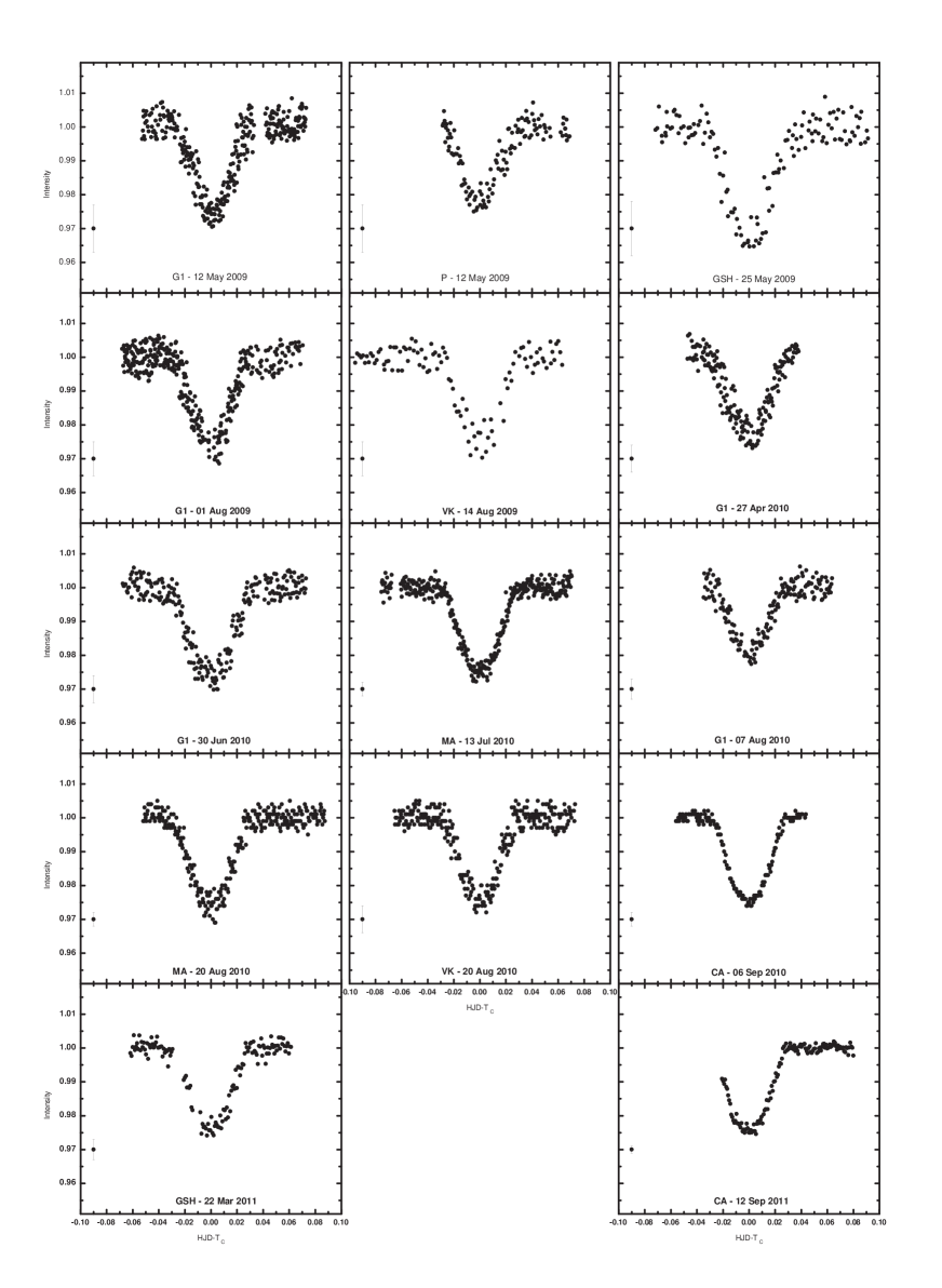
Figure 1: The light curves of the system TrES-3 obtained at individual observatories between May 2009 and September 2011. The best light curve (obtained at Calar Alto, Sep 2010) was used to determine system parameters. The data from other observatories were used for $T_{C}$ determination and TTV analysis. The typical error bar is plotted next to each light curve.

3 Light curve analysis

Our photometric observations of the TrES-3 system consist of data from different instruments and are of different photometric quality. For the purpose of radius determination, we decided to analyse only a light curve with the lowest scatter and the best rms = 1.2 mmag. We choose data obtained at Calar Alto observatory on September 06, 2010 (see Figs. 1 and 2). We first refined the light-curve system parameters and subsequently determined the individual times of transit as described below in order to improve ephemeris.

For the calculation of synthetic light curves we used two independent approaches: the first one is based on the routines from (Mandel & Agol, 2002) and the Monte Carlo simulations (described in Section 3.1), the second one uses JKTEBOP code (Southworth, Maxted & Smalley, 2004) (see Section 3.2).

3.1 SOLUTION 1

First we used the downhill simplex minimization procedure (implemented in routine AMOEBA, Press et al., 1992) to determine $4$ system parameters $R_{\mathrm{p}}/R_{*}$ (planet to star radius ratio), $i$ (inclination), $T_{C}$ (mid-transit time) and $R_{*}/a$ (star radius to semi-major axis ratio). The model light curve itself was computed via the analytic expressions from Mandel & Agol (2002). The quadratic limb darkening law was assumed and corresponding limb darkening coefficients $c_{1}$, $c_{2}$ were linearly interpolated from Claret (2000) assuming the stellar parameters from Sozzetti et al. (2009): $T_{\mathrm{eff}}$ = 5 650 K, $\log$ (g) = 4.4 and [Fe/H] = $-$0.19. As a goodness of the fit estimator we used the $\chi^{2}$ function:

$$\chi^{2}=\sum_{i=1}^{N}\left(\frac{m_{i}-d_{i}}{\sigma_{i}}\right)^{2},$$ (1)

where $m_{i}$ is the model value and $d_{i}$ is the measured value of the flux, $\sigma_{i}$ is the uncertainty of the $i^{\mathrm{th}}$ measurement and the sum is taken over all measurements. The orbital period and the limb darkening coefficients were fixed through the minimization procedure. The transit duration $T_{\mathrm{D}}$ was determined assuming the semi-major axis $a$ = 0.02282${}^{+0.00023}_{-0.00040}\,$au (Sozzetti et al., 2009). The parameters and the corresponding light curve for which we found the minimum value of $\chi^{2}$ function, are in Table 3 and Figure 2, respectively (SOLUTION 1).

To estimate the uncertainties of the calculated transit parameters, we employed the Monte Carlo simulation method (Press et al., 1992). We produced 10 000 synthetic data sets with the same probability distribution as the residuals of the fit in Figure 2. From each synthetic data set obtained by this way we estimated the synthetic transit parameters. The minimum $\chi^{2}_{\mathrm{min}}$ value corresponding to each set of Monte Carlo parameters was calculated as:

$$\chi^{2}_{\mathrm{min}}=\sum_{i=1}^{N}\left(\frac{m_{i}-s_{i}}{\sigma_{i}}\right)^{2},$$ (2)

where $m_{i}$ is the original best fit model value and $s_{i}$ is the ’Monte–Carlo simulated’ value. Figure 3 shows the dependence of the parameters $R_{\mathrm{p}}/R_{*}$ and $i$ on the reduced $\chi^{2}_{\mathrm{r}}$. This quantity is defined as:

$$\chi^{2}_{\mathrm{r}}=\frac{\chi^{2}_{\mathrm{min}}}{N-M},$$ (3)

where $N$ is the number of data points and $M$ is the number of fitted parameters. To fully understand the errors of the system parameters we constructed confidence intervals in 2-dimensional space. Figure 4 depicts the confidence regions for 2 parameters ($R_{\mathrm{p}}/R_{*}$ vs. $i$) as a projection of the original 4-dimensional region. The gray-colored data points stand for the $1\sigma$, $2\sigma$ and $3\sigma$ region with corresponding value of $\Delta\chi^{2}=\chi^{2}_{\mathrm{min}}-\chi^{2}_{\mathrm{m}}=4.72$, $9.7$ and $16.3$, respectively ($\chi^{2}_{\mathrm{m}}$ is the $\chi^{2}$ of the original best fit model value). From the shape of the dependence it could be seen that these two parameters correlate (see Section 3.3).

Finally, we took into account the uncertainty of the stellar mass and semi-major axis according to the simple error propagation rule. The results from the first analysis are shown in the Table 3 as SOLUTION 1.

3.2 SOLUTION 2 (JKTEBOP code)

We have modelled the light curve using the JKTEBOP code (Southworth, 2011) as well. JKTEBOP grew out of the original EBOP program written for eclipsing binary systems (Etzel, 1981; Popper & Etzel, 1981) via implementing the NDE (Nelson & Davis, 1972) model. JKTEBOP uses biaxial spheroids to model the component stars (or star and planet) and performs a numerical integration in concentric annuli over the surface of each body to obtain the flux coming from the system. This feature of the code allows us to avoid small and spherical planet approximations which are used in analytic light-curve generators based on Mandel & Agol (2002), and hence to derive planet’s oblateness. A model is fitted to the data by the Levenberg-Marquardt least-square procedure. The code converges rapidly toward a reliable solution and diminishes the correlation between fitted parameters (Southworth, 2008).

Figure 2: Top: The light curve obtained at Calar Alto on September 06, 2010, and the best fit corresponding by SOLUTION 1. Middle: Residuals from the best fit mentioned above. Bottom: Difference from the fits corresponding by SOLUTION 1 and SOLUTION 2.

The main parameters of a JKTEBOP fit are the orbital inclination $i$, and the fractional radii of the host star and planet, $r_{A}$ and $r_{b}$. The fractional radii are defined as:

$$r_{A}=\frac{R_{*}}{a},~{}~{}~{}~{}~{}~{}~{}~{}r_{b}=\frac{R_{p}}{a},$$ (4)

where $R_{*}$ and $R_{\mathrm{p}}$ are the stellar and planetary radii and $a$ is the orbital semi-major axis. Parameters $r_{A}$ and $r_{b}$ correspond to radii of spheres of the same volume as the biaxial spheroids. In JKTEBOP the fractional radii are reparametrized as their sum and ratio:

$$r_{A}+r_{b},~{}~{}~{}~{}~{}~{}~{}~{}k=\frac{r_{b}}{r_{A}}=\frac{R_{p}}{R_{*}},$$ (5)

because these are only weakly correlated with each other (Southworth, 2008). The directly fitted orbital inclination, $i$, allows the transit impact parameter $b$ = $\frac{a}{R_{*}}$ cos $i$ to be calculated. The initial values of parameters listed above were taken from Sozzetti et al. (2009). Because of different quality of data, the synthetic light curve was calculated only for the best light curve obtained at Calar Alto on September 06, 2010 (the same like in SOLUTION 1). A value of $a$ = 0.02282${}^{+0.00023}_{-0.00040}$ au (Sozzetti et al., 2009) was used in subsequent calculations. The best-fit model was used as a template and fitted to other light curves for which only the mid-transit time was allowed to vary. The resulting mid-transit times together with $T_{C}$ obtained from literature (Sozzetti et al., 2009; Gibson et al., 2009) are analysed in details in the Section 4. The determined parameters obtained by JKTEBOP code are presented in Table 3 as SOLUTION 2.

The errors of derived parameters were determined in two ways for each combination of data set and adopted LD law (we have used the same coefficients like in the case of SOLUTION 1). Firstly, we ran 1000 Monte Carlo (MC) simulations, a spread range of a given parameter within 68.3% was taken as its error estimate. Secondly, the prayer-bead method (e.g. Désert et al., 2011; Winn et al., 2009) was used to check whether red noise was present in our data. MC errors were found to be 2 – 3 times smaller than the values returned by the prayer bead method. This indicates that the light curve is affected not only by Poisson noise but also by additional correlated noise. Therefore, our prayer-bead error estimates were taken as our final errors.

Table 3: Parameters of the extrasolar system TrES-3 from this work (This work: SOLUTION 1 and SOLUTION 2) compared with the results from the previous studies. $R_{*}/a$ is the star radius to semi-major axis ratio, $R_{p}/R_{*}$ is the planet to star radius ratio, $i$ is the inclination of the orbit, $T_{D}$ is the transit duration assuming the semi-major axis of $a$ = 0.02282${}^{+0.00023}_{-0.00040}$ au (Sozzetti et al., 2009) and $P_{orb}$ is the orbital period. The orbital period in this work was fixed during analysis. The errors of the orbital periods are in parenthesis.

Source	$R_{*}/a$	$R_{p}/R_{*}$	$i$	$T_{D}$	$P_{orb}$
			$[\degr]$	[min]	[days]
O’Donovan et al. (2007)	0.1650 $\pm$ 0.0027	0.1660 $\pm$ 0.0024	82.15 $\pm$ 0.21	–	1.30619(1)
Sozzetti et al. (2009)	0.1687${}^{+0.0140}_{-0.0410}$	0.1655 $\pm$ 0.0020	81.85 $\pm$ 0.16	–	1.30618581(51)
Gibson et al. (2009)	–	0.1664${}^{+0.0011}_{-0.0018}$	81.73${}^{+0.13}_{-0.04}$	79.92${}^{+1.44}_{-0.60}$	1.3061864(5)
Colón et al. (2010)	–	0.1662${}^{+0.0046}_{-0.0048}$	–	83.77${}^{+1.15}_{-2.79}$	–
Southworth (2010)	–	–	82.07 $\pm$ 0.17	–	1.3061864(5)
Lee et al. (2011)	–	0.1603 $\pm$ 0.0042	81.77 $\pm$ 0.14	–	1.30618700(15)
Christiansen et al. (2011)	0.1664 $\pm$ 0.0204	0.1661 $\pm$ 0.0343	81.99 $\pm$ 0.30	81.9 $\pm$ 1.1	1.30618608(38)
Southworth (2011)	–	–	81.93 $\pm$ 0.13	–	1.30618700(72)
Sada et al. (2012)	–	–	–	77.9 $\pm$ 1.9	1.3061865(2)
Kundurthy et al. (2013)
Solution_1	0.1675 $\pm$ 0.0008	0.1652 $\pm$ 0.0009	81.95 $\pm$ 0.06	–	1.3062132(2)
Kundurthy et al. (2013)
Solution_2	0.1698 $\pm$ 0.0014	0.1649 $\pm$ 0.0015	81.51 $\pm$ 0.14	–	1.3062128(2)
Turner et al. (2013)	0.1721${}^{+0.0054}_{-0.0052}$	0.1693${}^{+0.0087}_{-0.0069}$	81.35${}^{+0.63}_{-0.51}$	81.30 $\pm$ 0.23	1.306 1854(1)
This work
Solution_1	0.1682 $\pm$ 0.0032	0.1644 $\pm$ 0.0047	81.86 $\pm$ 0.28	79.20 $\pm$ 1.38	1.306186
This work
Solution_2	0.1696${}^{+0.0024}_{-0.0027}$	0.1669${}^{+0.0027}_{-0.0025}$	81.76${}^{+0.14}_{-0.15}$	79.08 $\pm$ 0.72	1.306186

3.3 Light curve analysis results

The resulting values of the parameters together with their uncertainties are given in Table 3. For comparison, the parameters from previous studies are added there as well. Figure 2 shows the resulting best fit obtained by SOLUTION 1. In order to compare both solutions, we also plotted differences from the fit obtained by routines resulting from SOLUTION 1 and SOLUTION 2.

Figure 3: Top: Reduced $\chi^{2}_{\mathrm{r}}$ representing global minimum solution for calculated parameter $R_{\mathrm{p}}/R_{*}$. Bottom: Reduced $\chi^{2}_{\mathrm{r}}$ representing global minimum solution for calculated parameter $i$.

The final parameters are in good agreement with already published values. The output from SOLUTION 1, in particular $R_{\mathrm{p}}$ and $R_{*}$, correspond a bit better to parameters of Sozzetti et al. (2009) and Christiansen et al. (2011). The radii determined by JKTEBOP are also within the range of errors. Based on these two parameters we also inferred the critical value of inclination for total transit of TrES-3b as:

$${\rm cos}~{}i=\frac{R_{*}}{a}-\frac{R_{p}}{a}\Rightarrow i=81.9\degr.$$ (6)

As listed in Table 3, all values of inclination including uncertainties are in agreement with critical inclination calculated above. This is an evidence of grazing transit of TrES-3b.

We used MC simulations to produce of 10000 synthetic data sets with the same probability distribution as the residuals of the fit. From each synthetic data set we estimated the synthetic transit parameters. Using the results of the simulation, the dependence of the inclination versus the planet to star radius ratio is plotted in Figure 4. The figure demonstrates that there is a correlation between the parameters and that solution for the system TrES-3 is not unique and can be located in a relatively wide range (degeneracy of the parameters). This fact is also caused by grazing transit and by subsequent sensitivity of the solution to the determination of LD coefficients.

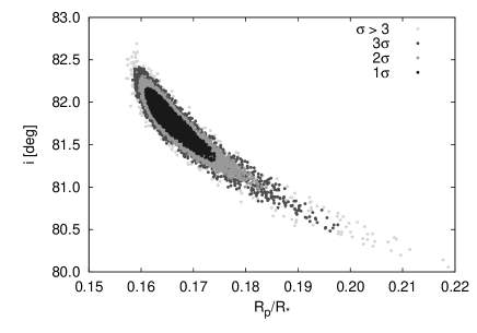
Figure 4: Confidence region depicted as a projection of the 4-dimensional region into 2-dimensional parameter space (inclination and ratio of the planet to star radius). Regions of $1\sigma$, $2\sigma$ and $3\sigma$ corresponding to $\Delta\chi=4.72$, $9.7$ and $16.3$, respectively, are marked with different gray colors.

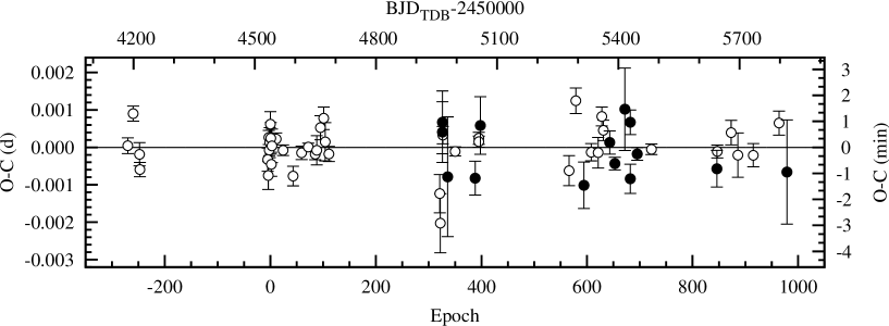
Figure 5: Observation minus calculation $O-C$ diagram for transit timing of TrES-3 b, plotted according to the new linear ephemeris. Open circles denote re-analysed mid-transit times from the literature. Filled symbols mark new mid-transit times reported in this paper.

For determination of our mid-transit times, the best-fit model was used as a template and fitted to other light curves for which only the mid-transit time was allowed to vary. In order to have homogeneous analysis of TTV, we collected the data points of transit light curves published in previous studies (see Figure 5). Transit light curve data of Sozzetti et al. (2009) and Colón et al. (2010) were available on-line and the remaining tabulated data were obtained from mentioned authors by e-mail. We re-analysed all transit light curves and derived mid-transit times by the same procedure (the code JKTEBOP) to get a homogeneous dataset for TTV analysis (see Section 4).

We also re-analysed all light curves under consideration with $k=r_{b}/r_{A}$ as a free parameter and tried to search for any variation. All determinations of $k$ were consistent within error bars with a mean value, so we did not detect any transit depth variation. We also saw no significant signal in periodograms.

4 Transit Timing Variation

Our new 14 mid-transit times and 42 redetermined literature values were used to refine the transit ephemeris. The mid-transit times were transformed from JD or HJD (based on UTC) into BJD (based on Barycentric Dynamical Time – TDB) using the on-line converter by Eastman, Siverd & Gaudi (2010). As a result of fitting a linear function of the epoch, we obtained the mid-transit time for the initial epoch $T_{0}=2454538.58144\pm 0.00007$ BJD_TDB and the orbital period $P_{\rm{b}}=1.30618599\pm 0.00000023$ d. The individual mid-transit errors were taken as weights. The linear fit yields reduced $\chi^{2}$ of $2.5$ that is similar to a value of 2.3 reported by Gibson et al. (2009). These values, noticeable greater than 1 might suggest the existence of an additional planet which perturbs the orbital motion of TrES-3 b (Sozzetti et al., 2009; Gibson et al., 2009).

Table 4: Results of transit timing. Obs. codes an observatory and instrument according to Table  1. $T_{0}$ denotes the mid-transit times given as BJD (based on Barycentric Dynamical Time, TDB). Errors of mid-transit times are in days. The $O-C$ values were calculated according to the new ephemeris.

Date	Obs.	Epoch	$T_{0}$ $(\rm{BJD_{\rm{TDB}}})$	$T_{0}$ error	$O-C$ (d)
2009 May 12	P	326	2454964.39885	0.00084	$+0.00077$
2009 May 12	G1	326	2454964.39859	0.00081	$+0.00051$
2009 May 25	GSH (CTK)	336	2454977.4593	0.0016	$-0.0007$
2009 Aug 01	G1	388	2455045.38091	0.00045	$-0.00070$
2009 Aug 14	VK	398	2455058.44418	0.00077	$+0.00071$
2010 Apr 27	G1	594	2455314.45510	0.00062	$-0.00082$
2010 Jun 30	G1	643	2455378.45937	0.00031	$+0.00034$
2010 July 13	MA	653	2455391.52067	0.00017	$-0.00022$
2010 Aug 07	G1	672	2455416.3397	0.0011	$+0.0012$
2010 Aug 20	MA	682	2455429.40118	0.00033	$+0.00090$
2010 Aug 20	VK	682	2455429.3997	0.0004	$-0.0006$
2010 Sep 06	CA	695	2455446.38075	0.00017	$+0.00005$
2011 Mar 22	GSH (STK)	846	2455643.6145	0.0005	$-0.0003$
2011 Sep 12	CA	979	2455817.3372	0.0014	$-0.0003$

Results for new mid-transit times are shown in Table 4. The observed minus calculated (O–C) diagram, plotted in Fig. 5, shows no significant deviation from the linear ephemeris. All our data points deviated by less than $3\sigma$. We also searched for a periodicity that could be a sign of an additional body in the system. We generated a Lomb–Scargle periodogram (Lomb, 1976; Scargle, 1982) for the residuals in a frequency domain limited by the Nyquist frequency and found the highest peak at $\sim$30 d and peak-to-peak amplitude of $70\pm 20$ s. This period could coincide with a stellar rotation period which is roughly estimated to be $\sim$28 d. Examples of such TTV signals induced by the stellar activity are observed in the Kepler data (e.g. Mazeh et al., 2013). However, the false alarm probability (calculated empirically by a bootstrap resampling method with $10^{5}$ trials) of the putative signal is disqualifying with a value of 18.2%. In addition, the amplitude is close to the mean 1-$\sigma$ timing error of our observations. These findings allow us to conclude that a strictly periodic TTV signal with the amplitude greater than $\sim$1 minute over a 4-year time span seems to be unlikely.

Following Gibson et al. (2009), we put upper constraints on a mass of a potential perturbing planet in the system with refined assumptions. We adopted a value of 1 min for the maximal amplitude of the possible TTV signal. We also increased the sampling resolution to probe resonances other than inner and outer 1:2 commensurabilities studied in detail by Gibson et al. (2009). We simplified the three-body problem by assuming that the planetary system is coplanar and initial orbits of both planets are circular. The masses of both the star and the transiting planet, as well as its semi-major axis were taken from Sozzetti et al. (2009). The orbital period of the hypothetical perturber was varied in a range between 0.2 and 5 orbital periods of TrES-3 b. We produced 2800 synthetic O–C diagrams based on calculations done with the Mercury code (Chambers, 1999). We applied the Bulirsch–Stoer algorithm to integrate the equations of motion.

Figure 6: The upper-mass limit of a hypothetical additional planet that could perturb the orbital motion of TrES-3b as a function of ratio of orbital periods of transiting planet, $P_{\rm{b}}$, and the hypothetical perturber, $P_{\rm{p}}$. Orbits located in a grey area were found to be unstable due to close encounters of both planets.

The most important feature of the Bulirsch-Stoer algorithm for N-body simulations is that it is capable of keeping an upper limit on the local errors introduced due to taking finite time-steps by adaptively reducing the step size when interactions between the particles increase in strength. Calculations covered 1500 days, i.e. a total time span of available transit observations. The results of simulations are presented in Fig. 6. Our analysis allows us to exclude an additional Earth-mass planet close to inner 1:3, 1:2, and 3:5 and outer 5:3, 2:1, and 3:1 mean-motion resonances (MMRs).

5 Long-term stability of the system

In this section, we investigated the long-term gravitational influence of TrES-3b planet on a potential second planet in the system. Thus, we performed numerical simulation for studying the stability of orbits and checking their chaotic behavior using the method of maximum eccentricity (e.g. Dvorak et al., 2003).

We used long-term integration of small-mass (Earth-mass) planet orbits for inspecting the stability regions in the TrES-3b system. The time span of the integration was around 140000 revolutions of the planet around the star. For the integration of this system we again applied an efficient variable-time-step algorithm (Bulirsch-Stoer integration method). The parameter $\epsilon$ which controls the accuracy of the integration was set to $10^{-8}$, in this case.

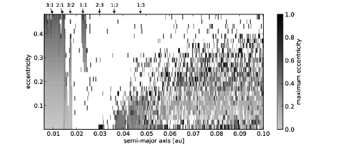
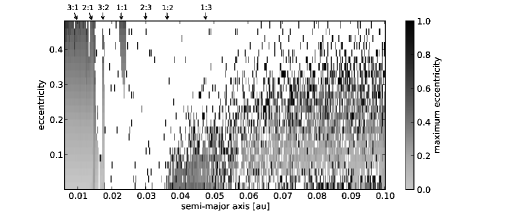
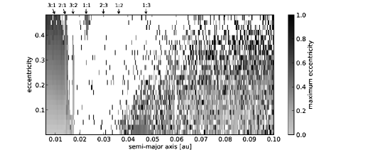
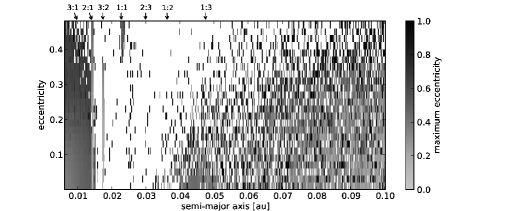
Figure 7: Stability plot in the $a-e$ plane showing the maximum eccentricity. From top left to bottom right: $i=5\degr$, $i=20\degr$, $i=35\degr$ and $i=50\degr$. The mean-motion resonances with TrES-3b planet are also marked. The minimal value of semi-major axis is 0.00625 au.

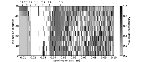
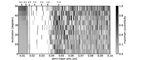
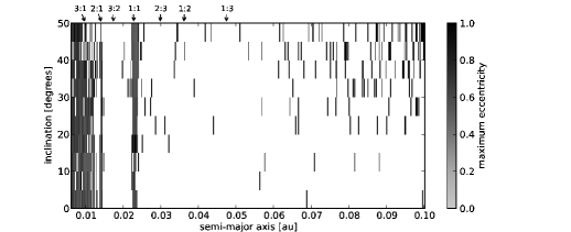
Figure 8: Stability plot in the $a-i$ plane showing the maximum eccentricity. From top left to bottom right: $e=0.001$, $e=0.1$, $e=0.3$ and $e=0.5$. The mean-motion resonances with TrES-3b planet are also marked. The minimal value of semi-major axis is 0.00625 au.

We have generated $10^{5}$ mass-less particles for representing small planets in this system. We assumed that semi-major axis ranges from 0.00625 au to 0.1 au. The inner border of the generated system of small planets is around 1.5 times star radius. This value of inner border is approximately at the location of Roche limit for a Earth-like planet and includes also the region in the vicinity of 3:1 MMR (0.01 au for this case) in our analysis. The step-size in semi-major axis was $\Delta\,a$ = 0.00025 au, in eccentricity $\Delta\,e$ = 0.02 and $\Delta\,i$ = 5$\degr$ in inclination. The upper limit of the grid in eccentricity was 0.5 and 50$\degr$ in inclination. We integrated the orbits of the small planets for the time-span of 500 years (about 140 000 revolutions of TrES-3b around the parent star). We obtained orbital evolution of each small planet in the system and also were able to study the stability regions at the end of the integration using the method of maximum eccentricity, mentioned above. The maximum eccentricity that the potential perturber of TrES-3b reached over the time of the integration is plotted on the $a-e$ ($a-i$) stability map in the Fig. 7 (Fig. 8).

Figure 7 shows the stability maps in $a-e$ plane for selected values of inclinations: $i=5\degr$, $i=20\degr$, $i=35\degr$ and $i=50\degr$ (from top left to bottom right). Also the MMRs with TrES-3b planet are marked in these plots. We can see a stable region inside the 2:1 MMR for each value of inclination. Outside the 2:1 MMR the gravitational influence of the TrES-3b planet is very strong and leads to depletion of these regions. Only the MMRs 2:1, 3:2 and 1:1 are moderately populated but the population decreases with the increase of the inclination. For completeness, we note that 5:3 ($a\approx$ 0.016 au) and 3:5 ($a\approx$ 0.032 au) MMRs are depleted and thus not stable for additional Earth-mass planet in their vicinity. In Fig. 8 we present the stability maps in $a-i$ plane for several values of eccentricities: $e=0.001$, $e=0.1$, $e=0.3$ and $e=0.5$. One can see the stable region inside the 2:1 MMR with TrES-3b planet, which we found stable also in the $a-e$ plane. Considering the region beyond the 1:3 MMR, the depletion of the planet population is not so strong than in the region between 2:1 and 1:3 MMR. This feature is in a good agreement with the weaker gravitational influence of the TrES-3b planet.

Based on our results, we showed that the region inside the TrES-3b planet orbit (especially inside the 2:1 up to 3:1 MMR) can be stable on longer timescales (hundreds of years or hundred thousands of revolutions of TrES-3b around the star) from the dynamical point of view. The region from 0.015 au (near 2:1 MMR) to 0.05 au (near 1:3 MMR) was found unstable apart from moderately populated MMRs located in this area (see figures Fig. 7 and Fig. 8). The relatively small increase of population in the mentioned MMRs depends on the initial values of semi-major axis, eccentricity and inclination. The region beyond the 0.05 au was found to have a chaotic behavior and the depletion of the planet population increases with increasing values of initial eccentricity as well as inclination.

6 Discussion and Conclusion

Based on the transit light curves obtained at several observatories between May 2009 and September 2011 we redetermined orbital parameters and the radius of the transiting planet TrES-3b. The best light curve (obtained at Calar Alto, Sep 2010) was used for light curve analysis, and the data from the other observatories were used for $T_{C}$ determination and TTV investigation. We used two independent solutions for parameters determination and finally, we concluded that our values are consistent with previous results of Sozzetti et al. (2009) and Christiansen et al. (2011).

The aim of this present paper was also to discuss possible presence of a second planet in the extrasolar system TrES-3. For this purpose we used our new 14 mid-transit times and the individual determinations from Sozzetti et al. (2009) and Gibson et al. (2009). The resulting $O-C$ diagram showed no significant deviation of data points from the linear ephemeris. In addition, we tried to search for a periodicity that could be caused by an additional body in the system. We can conclude that a strictly periodic TTV signal with the amplitude greater than 1 minute over a 4-year time span seems to be unlikely. This result, together with refined assumptions of Gibson et al. (2009) allow us to put upper constraints on the mass of a potential perturbing planet. The additional Earth-mass planet close to inner 3:1, 2:1, and 5:3 and outer 3:5, 1:2, and 1:3 MMRs can be excluded.

Finally, we used the long-term integration of the theoretical set of massless particles generated in TrES-3 system for studying the dynamical stability of potential second planet in the system (influenced by TrES-3b gravitation). From our analysis we found that the region inside the TrES-3b planet orbit (especially inside the 2:1 MMR) up to 3:1 MMR can be stable on longer timescales (hundreds of years or hundred thousands of revolutions of TrES-3b around the star) from the dynamical point of view. The region from 0.015 au (near 2:1 MMR) to 0.05 au (near 1:3 MMR) was found to be unstable apart from moderately populated MMRs located in this area. The relatively small increase of population in these MMRs depends on the initial values of semi-major axis, eccentricity and inclination. The region beyond 0.05 au was found to have a chaotic behavior and depletion of the planet population increases with increasing values of initial eccentricity as well as inclination.

References

- Broeg et al. (2005) Broeg C., Fernández M., Neuhäuser R. 2005, AN, 326, 134
- Chambers (1999) Chambers J.E. 1999, MNRAS, 304, 793
- Charbonneau et al. (2000) Charbonneau D., Brown T. M., Latham D. W., Mayor M. 2000, ApJ, 529, L45