A toy model to test the accuracy of cosmological N-body simulations

The evolution of an isolated over-density represents a useful toy model to test the accuracy of a cosmological N-body code in the non linear regime as it is approximately equivalent to that of a truly isolated cloud of particles, with same density profile and velocity distribution, in a non expanding background. This is the case as long as the system size is smaller than the simulation box side, so that its interaction with the infinite copies can be neglected. In such a situation, the over-density rapidly undergoes to a global collapse forming a quasi stationary state in virial equilibrium. However, by evolving the system with a cosmological code (GADGET) for a sufficiently long time, a clear deviation from such quasi-equilibrium configuration is observed. This occurs in a time $t_{LI}$ that depends on the values of the simulation numerical parameters such as the softening length and the time-stepping accuracy, i.e. it is a numerical artifact related to the limited spatial and temporal resolutions. The analysis of the Layzer-Irvine cosmic energy equation, confirms that this deviation corresponds to an unphysical dynamical regime. By varying the numerical parameters of the simulation and the physical parameters of the system we show that the unphysical behaviour originates from badly integrated close scatterings of high velocity particles.We find that, while the structure may remain virialized in the unphysical regime, its density and velocity profiles are modified with respect to the quasi-equilibrium configurations, converging however to well defined shapes, the former characterised by a Navarro Frenk White-type behaviour.

1 Introduction

In order to control the numerical integration accuracy of a finite self-gravitating system evolution in a static background one may use total energy and angular momentum conservation (Aarseth, 2003). In the cosmological case, instead of being conserved, the total (peculiar) energy decreases with time. Indeed, the cosmic energy equation, known as the Layzer-Irvine (LI) equation, describes the change of the total peculiar energy of a system due to the adiabatic expansion of the background (Peebles, 1980). The quantification of the deviations from the LI equation is one of the very first tests made in all cosmological codes (see, e.g., Teyssier (2001); Miniati & Colella (2007)). However, when typical initial conditions of standard models of structure formation are considered, the application of the LI test is limited by several reasons. First of all, high redshift initial conditions of typical cosmological N-body simulations are very uniform and cold, so that both the initial peculiar potential and kinetic energies are close to zero: this makes difficult the numerical estimation of the cosmic energy equation. In addition, at low redshifts, the density field is typically characterised by a great variety of non linear structures of different sizes and by low density regions still in the linear regime. Structures of different sizes and in different physical regimes give very different contributions to total the peculiar potential and kinetic energies so that it is not straightforward to estimate which error in the cosmic energy equation maybe tolerated and/or which constraints on the accuracy of the simulation maybe placed (see also discussion in Joyce & Sylos Labini (2013) and references therein).

For this reason several authors have developed convergence tests to explore the role of the various physical and numerical parameters that characterise a given simulation with the aim of establishing the reliability of the results (see e.g., Power et al. (2003)). Alternatively there are studies that compare different algorithms (see e.g., Knebe, Green & Benney (2003); Iannuzzi & Dolag (2011) and references therein). However, it is not a simple issue to control the numerical accuracy of the non-linear gravitational clustering in a cosmological simulation; for instance the question of determining the optimal spatial resolution, i.e. the best value for the gravitational force softening length, is still an open problem (see e.g., Splinter et al. (1988); Power et al. (2003); Romeo et al. (2008); Joyce, Marcos & Baertschiger (2009)).

In this paper, following the work of Joyce & Sylos Labini (2013), we consider the evolution of a very simple system, namely an isolated over-density in an expanding background, as a toy model to control the accuracy of the numerical integration and to test the correctness of a cosmological simulations.

The evolution of this kind of structure in a static background, has been studied since the earliest numerical N-body experiments (Hénon, 1964; van Albada, 1982; Aarseth et al., 1988; David & Theuns, 1989; Theuns & David, 1990; Bertin, 2000; Heggie & Hut, 2003; Boily & Athanassoula, 2006; Joyce, Marcos & Sylos Labini, 2009a; Sylos Labini, 2012). Briefly, driven by its own mean field, it collapses in a time scale $\tau_{c}\approx\sqrt{G\rho}^{-1}$, forming a virialized quasi-stationary state (QSS), i.e. a collision-less configuration that is not in thermodynamical equilibrium but that has a finite lifetime fixed by the collisional relaxation time-scale

$$\tau_{2}\approx\kappa N\tau_{c}\;,$$ (1)

where $N$ is the system particles number and $\kappa$ is a numerical factor that takes into account the “Coulomb logarithm” (Chandrasekhar, 1943; Theis & Spurzem, 1999; Diemand et al., 2004; Gabrielli et al., 2010).

Joyce & Sylos Labini (2013) have shown that an isolated over-density in a cosmological simulation should in principle evolve, in physical coordinates, just as if it were in a non-expanding space with open boundary conditions. This corresponds to the fact that such a structure is in the stable clustering regime. Namely, it evolves as it were truly isolated from the rest of universe. While the stable clustering regime is assumed to approximately describe the evolution of a structure in the strongly non-linear regime (Peebles, 1980), in the case of a single over-density with periodic boundary conditions and negligible finite size effects it must be precisely followed: the stable clustering regime thus corresponds to a QSS for a structure in a static background.

Indeed, in a cosmological simulation, where periodic boundary conditions are used, a single over-density can be considered isolated if finite size effects are negligible. Such mass distribution is isolated but for the interaction with its “copies” included in the infinite system over which the force is summed. It is easy to show that the copies contribute to the force with terms that represent perturbations suppressed by positive powers of $R_{0}/L$, where $R_{0}$ is the over-density size and $L$ is the side of the periodic box (Gabrielli et al., 2006; Joyce & Sylos Labini, 2013). When the latter condition is satisfied, the only difference in the evolution between the expanding and the static case can arise from the smoothing of the gravitational force.

Beyond the comparison of the expanding case with the template given by the static background evolution, one may consider the the analysis of the LI equation. In fact, Joyce & Sylos Labini (2013) found that is a useful diagnostic to control the accuracy of cosmological simulations when the evolution of a single over-density is considered. In this case, the breakdown of the LI test occurs when the structure leaves the stable clustering regime: this is due to the difficulty of numerically integrating the system evolution with sufficient accuracy because hard two-body collisions take place.

We consider in this paper the evolution of an initially spherical and uniform cloud of particles with a velocity dispersion such that the initial virial ratio is in the range $b_{0}\in[-1,0]$. When the system is warm enough, i.e. $b_{0}\approx-1$, it approximately maintains its original size and shape during and after the collapse. Instead, when the system is cold enough, i.e. $b_{0}\approx 0$, it undergoes to a stronger contraction so that its size is considerably reduced during the collapse forming thereafter a virialized structure with a density profile decaying as $r^{-4}$ (Joyce, Marcos & Sylos Labini, 2009a; Sylos Labini, 2012). Our goal is to study the collapse of such a single cloud of particles in an expanding universe: by monitoring the LI equation and the stability of the clustering (in real space) we may understand to which accuracy the cosmic energy equation must be satisfied, in the strongly non linear regime, so that the simulation still provides with physically meaningful results. In particular we will study the accuracy of the numerical integration by changing the numerical and physical parameters that characterise a simulation.

The paper is organised as follows. In Sect.2 we recall the main results of the evolution of an isolated over-density in a static background. Then we summarise the results of Joyce & Sylos Labini (2013) concerning the approximate equivalence of an isolated cloud of particles in a static background with open boundary conditions and the same cloud when it is placed alone in a box of an infinite periodic system with space expansion — i.e., when the simulation is run in cosmological conditions. In Sect.3 we discuss the preparation of the initial conditions, the choice of the parameters that control the numerical integration and we briefly recall the LI test. The comparison between the evolution of an isolated over-density in a static and expanding background is presented in Sec.4. A series of systematic tests to determine the role of the integration parameters such as the gravitational force softening length and the accuracy of the time-stepping is presented in Sect.5. Then in Sect.6 we discuss several tests performed by changing the physical parameters of the initial conditions, such as the number of particles, the system size and the velocity dispersion. Finally in Sect.7 we discuss the principal results and then we draw our main conclusions.

2 Isolated over-density in a cosmological and a static background

Firstly we briefly recall the main features of the collapse of an isolated over-density in a static background with open boundary conditions (hereafter STAT case). Then we discuss the equivalence of the evolution of an isolated structure in STAT case and in an expanding background with periodic boundary conditions (EXP case).

2.1 Isolated over-densities in a static background

In the STAT case, the global collapse of an isolated and spherical cloud of self-gravitating particles, of density $\rho$, is determined by its mean gravitational field and it is characterised by the time scale

$$\tau_{c}=\sqrt{\frac{3\pi}{32G\rho}}\;.$$ (2)

When the initial velocity dispersion is such that the virial ratio is $b_{0}=2K_{0}/W_{0}\approx-1$ (where $K_{0}/W_{0}$ is the system initial kinetic/potential energy) the collapse consists in a few oscillations that drive the system to a virialized QSS: this maintains approximately the size $R_{0}$ and shape of the initial configuration (Sylos Labini, 2012).

On the other hand, when the initial velocity dispersion is small enough (or zero), the system undergoes to a stronger contraction reducing its size by a large factor. In this case the features of the virialized QSS depend explicitly on the number of system particles (at constant density): for instance, when particles are initially Poisson distributed, the intrinsic characteristic size in Eq.3 scales as $r_{c}\approx N^{-1/3}$ (Aarseth et al., 1988; Joyce, Marcos & Sylos Labini, 2009a). Other noticeable features are: (i) during the collapse a fraction of particles gain enough kinetic energy to escape from the system; (ii) the density profile after the collapse is characterised by the power law decay described by

$$n(r)=\frac{n_{c}}{1+(r/r_{c})^{4}}\;,$$ (3)

(that we denominate the quasi equilibrium profile — QEP) where $r_{c}$ and $n_{c}$ are two constants.

The key to understand the formation of this density profile is represented by the physics of the ejection mechanism. The main characteristics of the virialized QSS that can be framed in a simple physical model introduced by Sylos Labini (2012) are

$$n(r)\sim r^{-4}\;,$$ (4)

$$\sigma^{2}_{r}(r)\equiv\langle v_{r}^{2}\rangle\sim r^{-1}\;,$$ (5)

$$\Phi(r)\equiv\frac{n(r)}{\sigma^{3}_{r}(r)}\sim\frac{r^{3/2}}{r^{4}}\sim r^{-5/2}\;,$$ (6)

where $v_{r}$ is the radial velocity and $\Phi(r)$ is the so-called pseudo phase-space density. Note that, once the QSS is formed, its potential and kinetic energy reach a constant value: this fact represents one of the diagnostics to numerically detect the quasi stationarity of the particle configuration (Joyce, Marcos & Sylos Labini, 2009a; Sylos Labini, 2012; Joyce & Sylos Labini, 2013).

2.2 Equivalence of the evolution in a static and in an expanding background

Joyce & Sylos Labini (2013) have shown that when a cosmological code is used to simulate an isolated structure (of size $R_{0}$) in an expanding universe, it should reproduce the same results, in physical coordinates, as that obtained for the same structure in open boundary conditions without expansion. Let us briefly recall in which limit this equivalence is verified.

Dissipation-less cosmological N-body simulations solve numerically the equations (Peebles, 1980)

$$\frac{d^{2}{\bf x}_{i}}{dt^{2}}+2H\frac{d{\bf x}_{i}}{dt}=-\frac{1}{a^{3}}Gm\sum^{copies}\sum_{j\neq i}^{j=1,..N}\frac{{\bf x}_{i}-{\bf x}_{j}}{|{\bf x}_{i}-{\bf x}_{j}|^{3}}$$ (7)

where ${\bf x}_{i}$ are the comoving particle coordinates of the $i=1,...,N$ particles of equal mass $m$, enclosed in a cubic box of side $L$, and subject to periodic boundary conditions, $a(t)$ is the appropriate scale factor for the cosmology considered, and $H(t)={\dot{a}}/{a}$ is the Hubble constant. Note that the force on a particle is that due to the $N-1$ other particles and to all their copies. The leading non-zero term of the force due to the copies is a repulsive “dipole”; by neglecting the quadrupole and higher multipole terms, that are convergent and suppressed by positive powers of $(R_{0}/L)$ compared to the dipole term (Gabrielli et al., 2006; Joyce & Sylos Labini, 2013), we can rewrite Eq.7 as

$$\frac{d^{2}{\bf x}_{i}}{dt^{2}}+2H\frac{d{\bf x}_{i}}{dt}=-\frac{Gm}{a^{3}}\sum_{j\neq i}^{j=1,..N}\frac{{\bf x}_{i}-{\bf x}_{j}}{|{\bf x}_{i}-{\bf x}_{j}|^{3}}+\frac{4\pi G\rho_{0}}{3}{\bf x}_{i}$$ (8)

where the sum is now only over the $N-1$ particles in the simulation box. Assuming for simplicity an Einstein-de Sitter (EdS) cosmology, for which

$$\frac{\ddot{a}}{a}=-\frac{4\pi G\rho_{0}}{3a^{3}}\,,$$ (9)

Eq.7 may be written, in physical coordinates ${\bf r}_{i}\equiv a(t){\bf x}_{i}$, simply as

$$\frac{d^{2}{\bf r}_{i}}{dt^{2}}=-Gm\sum_{j\neq i}^{j=1,..N}\frac{{\bf r}_{i}-{\bf r}_{j}}{|{\bf r}_{i}-{\bf r}_{j}|^{3}}\;.$$ (10)

These are the equations of motion of $N$ purely self-gravitating particles. Therefore, up to finite size corrections that vanish in the limit $R_{0}/L\rightarrow 0$, the equations of motion (in physical coordinates) in an expanding universe are the same of those describing the evolution of the same finite structure in a static background with open boundary conditions.

We stress that Eq.10 represents an important approximation that justifies the analogy between the same cloud of self-gravitating particles in STAT and EXP conditions. This is not a trivial approximation as it consists in replacing the sum in Eq.7 on a infinite periodic system, i.e. with infinite terms, with the sum on a finite system in Eq.10. The periodic sum can be written as a local sum on $N$ particles and a non-local term which takes into account the contribution of the infinite copies: this latter term can be neglected for the system considered, i.e. for $R_{0}<L$. Only in this situation the evolution of a single over-density in a periodic system, i.e., an infinite number of over-densities one in each of the infinite boxes of the periodic system, in an expanding background is equivalent to the evolution of a truly isolated over-density in a static background with open boundary conditions.

Note that the simulations are run, as usual, in comoving coordinates. In what follows we present analyses both in comoving and in physical coordinates because the stable clustering regime should manifest itself in physical coordinates, i.e. the structure remains almost invariant only in these coordinates (Joyce & Sylos Labini, 2013).

3 The simulations

3.1 Initial conditions

We have considered a system with total mass $M$ in a spherical volume $V=4\pi/3R_{0}^{3}$: this can be discretized by using $N$ randomly distributed particles of mass $m$ such that

$$\rho=\frac{M}{V}=\frac{3Nm}{4\pi R_{0}^{3}}=\mbox{const.}$$ (11)

We have used $10^{3}\leq N<10^{4}$ (series S), $N=10^{4}$ (series M) and $10^{4}<N\leq 10^{5}$ (series L). Details of the simulations are reported in Table 1: all length scales are given in units of the box side $L$. Note that the results we report require only choice of units for length and energy: for the former we will take units defined by $L=1$, and for the latter units in which $W_{0}=3GM^{2}/(5R_{0})=-1$, i.e. in which the initial continuum limit gravitational potential energy is minus unity.

Name	$N$	$|b_{0}|$	$R_{0}$	$\varepsilon$	$\varepsilon/\ell$	$\eta$
S1a	1E3	0	1.0E-1	3.7 E-6	4.2E-4	2.5E-2
S4a	1E3	0	1.0E-1	3.7 E-5	4.2E-3	2.5E-2
S4b	2E3	0	1.0E-1	3.7 E-5	5.3E-3	2.5E-2
S4c	4E3	0	1.0E-1	3.7 E-5	6.6E-3	2.5E-2
S4d	6E3	0	1.0E-1	3.7 E-5	7.6E-3	2.5E-2
S4e	8E3	0	1.0E-1	3.7 E-5	8.3E-3	2.5E-2
S4f	1E3	0	1.0E-1	3.7 E-5	8.3E-3	2.5E-3
S4g	1E3	0	1.0E-1	3.7 E-5	8.3E-3	5.0E-4
S6a	1E3	0	1.0E-1	3.7 E-4	4.2E-2	2.5E-2
M1a	1E4	0	1.0E-1	3.7 E-6	9.0E-4	2.5E-2
M1b	1E4	0	1.0E-1	3.7 E-6	9.0E-4	5.0E-3
M1c	1E4	0	1.0E-1	3.7 E-6	9.0E-4	1.3E-2
M1d	1E4	0	1.0E-1	3.7 E-6	9.0E-4	2.5E-2
M1e	1E4	0	1.0E-1	3.7 E-6	9.0E-4	1.3E-1
M1f	1E4	0	1.0E-1	3.7 E-6	9.0E-4	2.5E-1
M2a	1E4	0	1.0E-1	7.4 E-6	1.8 E-3	2.5E-3
M3a	1E4	0	1.0E-1	1.0 E-5	2.4 E-3	2.5E-2
M4a	1E4	0	1.0E-1	3.7 E-5	9.0 E-3	2.5E-2
M4b	1E4	0	1.0E-1	3.7 E-5	9.0 E-3	2.5E-2
M4c	1E4	0	1.0E-1	3.7 E-5	9.0 E-3	2.5E-2
M4d	1E4	0.25	1.0E-1	3.7 E-5	9.0 E-3	2.5E-2
M4e	1E4	0.5	1.0E-1	3.7 E-5	9.0 E-3	2.5E-2
M4f	1E4	0.75	1.0E-1	3.7 E-5	9.0 E-3	2.5E-2
M4g	1E4	1.0	1.0E-1	3.7 E-5	9.0 E-3	2.5E-2
M4h	1E4	0	2.5E-2	3.7 E-5	3.7 E-2	2.5E-2
M4k	1E4	0	5.0E-2	3.7 E-5	1.7 E-2	2.5E-2
M4i	1E4	0	2.0E-1	3.7 E-5	4.4 E-3	2.5E-2
M4j	1E4	0	3.0E-1	3.7 E-5	3.0 E-3	2.5E-2
M4l	1E4	0	1.0E-1	3.7 E-5	9.0 E-3	2.5E-3
M4m	1E4	0	1.0E-1	3.7 E-5	9.0 E-3	5.0E-3
M4n	1E4	0	1.0E-1	3.7 E-5	9.0 E-3	5.0E-2
M4o	1E4	0	1.0E-1	3.7 E-5	9.0 E-3	1.0E-1
M5a	1E4	0	1.0E-1	7.4 E-5	1.8 E-2	2.5E-2
M6a	1E4	0	1.0E-1	3.7 E-4	9.0 E-2	2.5E-2
M6b	1E4	0	2.5E-2	3.7 E-4	3.7 E-1	2.5E-2
M6c	1E4	0	5.0E-2	3.7 E-4	1.8 E-1	2.5E-2
M6d	1E4	0	2.0E-1	3.7 E-4	4.5 E-2	2.5E-2
M6e	1E4	0	3.0E-1	3.7 E-4	3.0 E-2	2.5E-2
M7a	1E4	0	1.0E-1	7.4 E-4	1.8 E-1	2.5E-2
M8a	1E4	0	1.0E-1	3.7 E-3	9.0 E-1	2.5E-2
L4a	2E4	0	1.0E-1	3.7 E-5	1.1 E-2	2.5E-2
L4b	4E4	0	1.0E-1	3.7 E-5	1.4 E-2	2.5E-2
L4c	6E4	0	1.0E-1	3.7 E-5	1.6 E-2	2.5E-2
L4d	8E4	0	1.0E-1	3.7 E-5	1.8 E-2	2.5E-2
L4e	1E5	0	1.0E-1	3.7 E-5	1.9 E-2	2.5E-2

Table 1: Details of the N-body simulations: $N$ is the number of particles in the spherical over-density, $|b_{0}|$ is the absolute value of its initial virial ratio, $R_{0}$ is its initial radius, $\varepsilon$ is the softening length, $\ell$ is the initial average distance between nearest neighbours and $\eta$ is the parameter that control the accuracy of the time-stepping. Only in the case of the simulation M4b (M4c) we have changed the parameter $\theta$ from 0.7 to 0.1 (the parameter $\phi$ from $5\times 10^{-3}$ to $5\times 10^{-4}$). (See Sect.3.2 for a discussion of the various numerical parameters of the code, i.e. $\varepsilon,\eta,\theta,\phi$).

Note that the system radius $R_{0}$ is chosen to be $R_{0}<L/4$ so to minimise, as discussed above, the effect of the periodic boundary conditions. In particular, the distance between any pair of structure particle $i,j$ is less than that separating $i$ from any particle of the copies in the infinite periodic system.

The spherical cloud corresponds, in a cosmological simulation, to an over-density with initial mass density contrast

$$\delta=\frac{\rho}{\rho_{0}}=\frac{3L^{3}}{4\pi R_{0}^{3}}\;,$$ (12)

where $\rho=3M/(4\pi R_{0}^{3})$ is the cloud density and $\rho_{0}=M/L^{3}$ is the mean mass density of the universe (see Tab.2). Particles mass is such that $\rho_{0}$ is equal to the critical density.

$R_{0}$	$\delta$	$4/(3\pi)\sqrt{\delta}$	$\ell$
0.025	15360	52.6	1.0E-3
0.05	1920	18.6	2.1E-3
0.1	240	6.6	4.1E-3
0.2	30	2.3	8.2E-3
0.3	8.9	1.1	1.2E-2

Table 2: Parameters of the spherical clouds with different initial radius $R_{0}$ and with over-density $\delta$ (Eq.12). The third column reports the pre-factor of Eq.14. The average distance between nearest neighbours $\ell$ is computed for $N=10^{4}$, i.e. $\ell\approx 4.12\times 10^{-2}R_{0}$.

The scale factor in an EdS universe obeys to (Peebles, 1980)

$$a(t)=a_{0}\left(\frac{t}{t_{0}}\right)^{2/3}\;,$$ (13)

where $t_{0}=1/\sqrt{6\pi G\rho_{0}}$. Assuming $a_{0}=1$ from Eqs.12-13 we find (Joyce & Sylos Labini, 2013)

$$t-t_{0}=[a^{3/2}-1]t_{0}=\frac{4}{3\pi}\sqrt{\delta}\,[a^{3/2}-1]\tau_{c}$$ (14)

where $\tau_{c}$ is given by Eq.2. Note that from Eq14 we find that only for very high values of the over-density, i.e. $\delta>10^{4}$, at moderate expansion factors $a\approx 10$, $(t-t_{0})/\tau_{c}$ is of the order of a thousand i.e. of the order of $\tau_{2}$ for $N=10^{3}$ (see Eq.2).

3.2 Numerical integration parameters

We have used the publicly available tree-code GADGET (Springel et al., 2001; Springel, 2005). In this code one may choose the values of a number of parameters and we have followed the prescriptions of the user guide for GADGET-2 to fix the basic ones.

The gravitational potential used by GADGET has the exact Newtonian potential above a separation of $2.8\varepsilon$ while for smaller separations the potential first derivative vanishes . The different values of $\varepsilon$ used are reported in Tab.1. Note that we have chosen a softening length that is fixed in comoving coordinates and thus it varies in physical ones.

Further we have set, following Power et al. (2003); Springel (2005) a Barnes-Hut opening criterion with an opening angle of the tree algorithm $\theta=0.7$ for the first force computation and a dynamical updating criterion thereafter . The accuracy of the relative cell-opening criterion (i.e., the parameter ErrTolForceAcc)  is set to $\phi=5\times 10^{-3}$. Finally, we have chosen the time-stepping criterion 0 of GADGET where the value of the parameter controlling its accuracy $\eta$ (i.e., the parameter ErrTolIntAccuracy) is reported in Tab.1.

3.3 Basic definitions

Let us introduce some basic definitions that will be useful in what follows. The kinetic energy in physical coordinates is

$$K_{p}=\frac{1}{2}\sum_{i=1,N}m\left(\frac{d{\bf r}_{i}}{dt}\right)^{2}$$ (15)

and the potential energy in physical coordinates is

$$W_{p}=\frac{1}{2}\sum_{i=1,N}m_{i}\Phi({\bf r}_{i})$$ (16)

where

$$\Phi({\bf r}_{i})=-G\sum_{j=1,N}^{j\neq i}m_{j}g(|{\bf r}_{i}-{\bf r}_{j}|)$$ (17)

and where $g(r)$ is the exact GADGET pair potential (Springel, 2005). The virial ratio is defined as

$$b=\frac{2K_{p}}{W_{p}}\;.$$ (18)

Note that the initial virial ratio is $b_{0}=2K_{0}/W_{0}$, where $K_{0},W_{0}$ are respectively the initial kinetic and potential energy. We define the potential energy in comoving coordinates

$$W_{c}=\frac{1}{2}\sum_{j}m_{j}\Phi({\bf x}_{i})=W_{p}\times a$$ (19)

and the GADGET gravitational potential energy

$$W_{g}=\frac{1}{2}\sum_{j=1,N}^{copies}m_{j}\Phi({\bf x}_{i})\;,$$ (20)

i.e., the two-body potential is calculated by using periodic boundary conditions. As mentioned above, in the limit $R_{0}\ll L$, we have $W_{g}\approx W_{c}$.

The peculiar kinetic energy is

$$K_{c}=\frac{1}{2}\sum_{i}m_{i}|{\bf v}_{i}|^{2}$$ (21)

where

$${\bf v}_{i}=a(t)\frac{d{\bf x}_{i}}{dt}=\frac{d{\bf r}_{i}}{dt}-H(t){\bf r}_{i}\;.$$ (22)

If the system is virialized in a region of size $R_{0}\ll L$ then

$$\left(\frac{d{\bf r}_{i}}{dt}\right)^{2}\sim\frac{GM}{R_{0}}\gg H^{2}(t){\bf r}_{i}^{2}\approx G\rho_{0}R_{0}^{2}\;.$$ (23)

In this approximation

$$\frac{d{\bf r}_{i}}{dt}\approx{\bf v}_{i}$$ (24)

so that the kinetic energy in physical coordinates (Eq.15) is well approximated by the peculiar kinetic energy (Eq.21), i.e. $K_{p}\approx K_{c}$.

3.4 The Layzer-Irvine equation

Let us briefly recall the expression of the LI equation. By defining the total peculiar energy as $\tilde{E}=(K_{c}+W_{p})$ the LI equation can be written as

$$\frac{d(a\tilde{E})}{da}=-K_{c}\;.$$ (25)

Integrating Eq.25 we find

$$A(a)=\ \frac{|a\tilde{E}(a)-a_{0}\tilde{E}(a_{0})|}{\int_{a_{0}}^{a}K_{c}(a)da}=1\;.$$ (26)

In order to test whether the LI equation is numerically satisfied during the time integration, one may measure the deviation of $A(a)$ from 1. In particular, we will determine the expansion factor $a_{LI}$ such that

$$|A(a_{LI})-1|<0.1\;\;\mbox{for}\;\;a<a_{LI}\;,$$ (27)

and larger than 0.1 for $a>a_{LI}$. This allows us to quantitatively determine the range of redshifts in which the LI equation is well approximated in the simulations, i.e. in which the LI test is satisfied. Note that at very early times, when the initial velocities are close (or equal) to zero the denominator of Eq.26 approaches zero and thus $A(a)$ is difficult to be precisely determined. Otherwise for long enough times there is not any particular numerical problem in the determination of Eq.26.

4 Comparison between the evolution in a static and expanding background

We first compare the evolution of an isolated and uniform over-density in an expanding background with periodic boundary conditions (EXP) with the evolution of the same system in a static background and with open boundary conditions (STAT). We consider here the simulation M4a (see Tab.1), which we have chosen as a reference for the reasons illustrated below. Results for the other simulations are discussed in the next sections.

Note that the difficulty of integrating the cold collapse occurs only around the strongest collapse phase of the system, i.e. at $t\approx\tau_{c}$, a time scale which is much smaller than any relevant value of the expansion factor considered in the what follows.

4.1 Short time evolution

Fig.1 (upper panel) shows the potential and kinetic energy in physical coordinates (normalised to the initial potential energy $W_{0}$). As for the STAT case the potential (kinetic) energy decreases (increases) to reach its minimum (maximum) at $t\approx\tau_{c}$, i.e. at the strongest phase of the collapse. For $t>\tau_{c}$ the bounded structure is stationary, i.e. $W_{p}\approx$ const., and it satisfies the virial equilibrium (Fig.1 — bottom panel). A fraction of about $f_{p}\approx 25\%$ of the particles gain kinetic energy so that, after the collapse, they are ejected from the system moving as free particles thereafter.

Energy conservation for the STAT case can easily be controlled to a precision better than $\approx 0.01\%$ (see, e.g., Aarseth (2003) and references therein). From the LI test (Fig.1 — bottom panel) in the EXP case we find $A(t)\approx 1$ with relatively large fluctuations up to the maximum contraction phase. However, these fluctuations are damped after the collapse: we thus conclude that in this range of time the system is still in the regime $a<a_{LI}$ (see Eq.27).

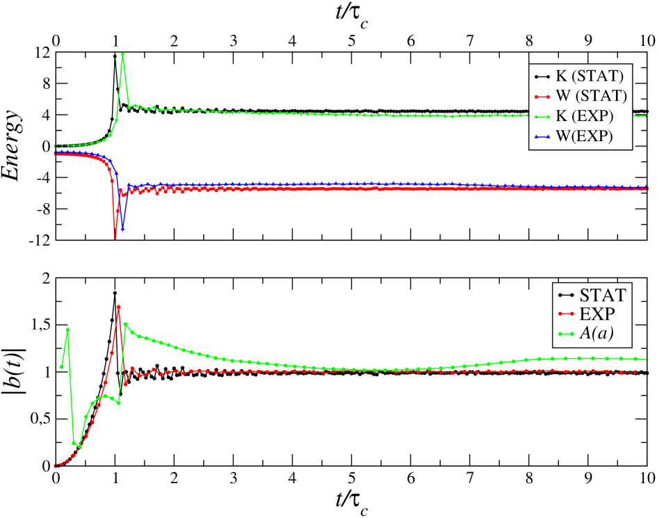
Figure 1: Upper panel: Energy in physical coordinates ($K_{p}$ Eq.15 and $W_{p}$ Eq.16) normalised to the initial total energy as a function of time (computed by using Eq.14 for the EXP case), together with the corresponding behaviour of the same system in the STAT case. Bottom panel: virial ratio $|b(t)|$, together with the LI test (Eq.26) for the EXP case.

The density profile (Fig.2 — upper panel) is well fitted by Eq.3 both in the EXP and STAT case. The radial velocity dispersion (Fig.2 — bottom panel) shows the Keplerian behaviour described by Eq.5 Therefore the pseudo phase-space density obeys to Eq.6, i.e. it decays as $\Phi(r)\sim r^{-5/2}$.

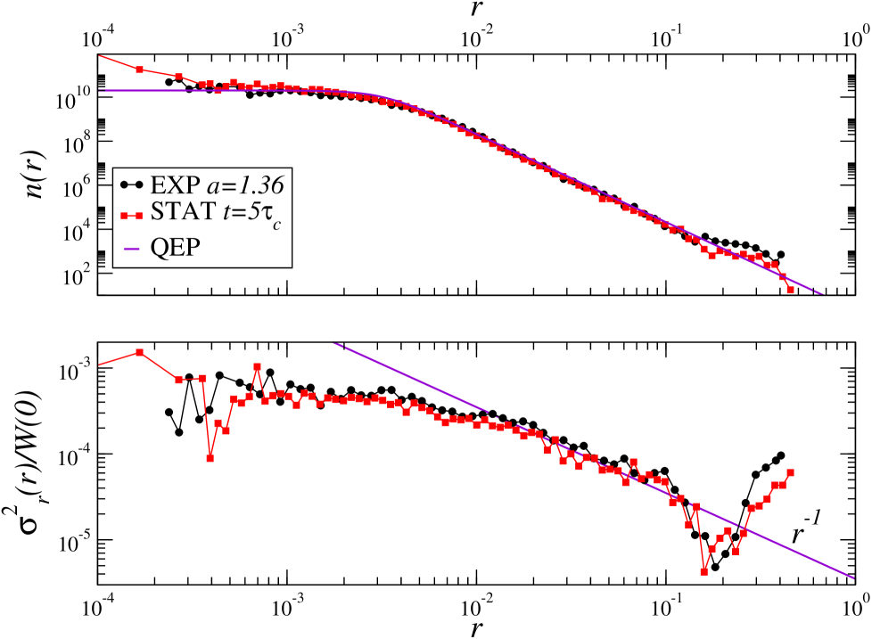
Figure 2: Comparison of the density (upper panel) and velocity (bottom panel) profiles of the same system evolved in an expanding background (EXP at $a=1.36$ — black circles) and in a static background with open boundary conditions (STAT at $t=5\tau_{c}$ — red squares). The best fit with Eq.3 (QEP) and a line with slope $-1$ are shown as references (see Eq.5).

4.2 Long time evolution

The situation discussed in Sect.4.1 drastically changes at longer times in the EXP simulation. Indeed, already for moderate values of the expansion factor, the evolution of the system rapidly deviates from the short-time behaviour, and correspondingly the properties of the QSS become different from Eqs.4-6.

We find that $W_{p}\approx$ const., i.e. the structure is in a QSS and in the stable clustering regime, only for $a<a_{LI}\approx 6$ (see Fig.3). Instead, for $a>a_{LI}$ we find that $|W_{p}|\sim 1/a$ (and thus $W_{c}\approx$ const). Thus the breakdown of the LI test corresponds to a departure from the stable clustering regime.

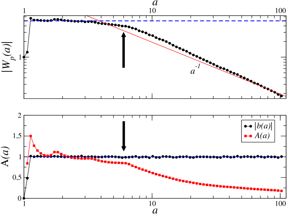
Figure 3: Upper panel: Absolute value of the potential energy in physical coordinates $W_{p}(a)$ (Eq.16) as a function of the scale factor. The approximate value of $a_{LI}$, separating the regime where $W_{p}\approx$ const. from the one where $|W_{p}|\sim a^{-1}$, is reported as reference. Bottom panel: LI test (Eq.26) and virial ratio (absolute value) for particles with negative energy.

Indeed, the density profile in comoving coordinates for $a>a_{LI}$ stabilises to an almost “asymptotic” shape which does not change anymore at small radii and slowly changes at large ones (see Fig.4). This is characterised by an approximate $x^{-3}$ decay extending over about three decades, i.e. from $\sim 10^{-3}L$ to $L$.

Note that the softening length is fixed in comoving coordinates and thus in physical coordinates it increases as $\varepsilon_{p}=a\varepsilon$. When the structure is in the stable clustering regime, its size in physical coordinates $R_{p}$ is constant, and thus $R_{p}/\varepsilon_{p}\propto 1/a$: if the stable clustering regime persists long enough then the size of the structure will become of the order of, or even smaller than, the softening length. However, we noticed that beyond a certain time the structure becomes stable in comoving coordinate and thus its size in physical coordinates scales as $R^{*}_{p}=aR^{*}_{cc}$, where $R^{*}_{cc}$ is the constant size in comoving coordinates. Therefore for $a>a_{LI}$ one approximately finds that $R^{*}_{p}/\varepsilon_{p}\approx R^{*}_{cc}/\varepsilon\approx const.$

The length scale $R^{*}_{cc}$ can be estimated, for instance, by measuring the radius $R(0.4)$ ($R(0.8)$) including the 40% (80%) of the mass of the virialized structure. As shown in inset panel of Fig.4, for $a>a_{LI}$, $R(0.4)$ and $R(0.8)$ remain respectively larger than 10 and 100 times the scale beyond which the force is exactly Newtonian, i.e. 2.8$\varepsilon$. In this condition the virial ratio fluctuates around -1 at all times (see Fig.3). This implies that the Newtonian value of the mean field potential is well approximated by the smoothed potential and thus the softening length does not perturb the mean field dynamics. (Note that this result is confirmed by the behaviours measured by using other values of the softening length, as well as by an analysis of the gravitational potential energy in function of $\varepsilon$ — see discussion in Sect.5.1).

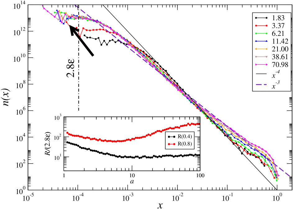
Figure 4: Evolution of the density profile in comoving coordinates. Two reference lines with slope -4 and -3 are reported as a reference. The arrow shows the direction of the density profile evolution. Inset panel: behaviours in function of the scale factor of the length scale $R(0.4)$ ($R(0.8)$), including the $40\%$ ($80\%$)of the mass of the virialized structure, normalised to $2.8\varepsilon$.

Coherently with the behaviour of the energy, the density profile in physical coordinates (see Fig.5) does not change for $a<a_{LI}$, and it is well fitted by Eq.3: this situation corresponds to the QSS in the stable clustering regime. Note that, as time passes, the spatial extension of the halo, i.e. the range of radii where $n(r)\sim r^{-4}$, increases. Indeed, as time passes particles with energy $e_{p}\mathrel{\hbox to0.0pt{\lower 3.0pt\hbox{$\mathchar 536\relax$}\hss}\raise 2.0pt\hbox{$\mathchar 316\relax$}}0$ may go asymptotically far from the structure core (Sylos Labini, 2012).

On the other hand, for $a>a_{LI}$, we find that $n(r)$ continues to evolve: at large radii it decays as $\sim r^{-3}$ and at small radii the density does not flatten as for the STAT case. A Navarro, Frenk & White (1997) (NFW) profile

$$n(r)=\frac{n_{c}}{(r/r_{c})(1+(r/r_{c}))^{2}}\;.$$ (28)

gives a reasonable fit for $a>a_{LI}$ (bottom panels of Fig.5): in particular the large scale tail shows a well-defined $r^{-3}$ decay. Therefore only when stability in physical coordinates is observed, the density profile is consistent with the expected one, i.e. Eq.3; when stability in physical coordinates is broken then the density profile changes its functional behaviour approaching the NFW one.

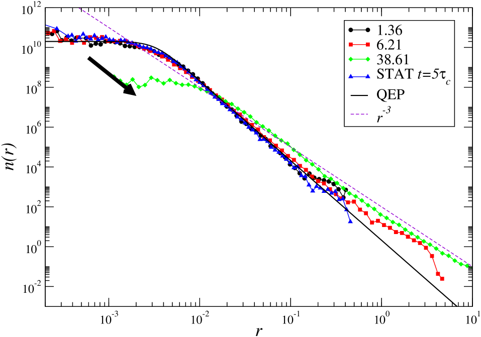
Figure 5: Density profile in physical coordinates for the simulation M4a at different scale factors $a$ (see labels) together with the density profile for the STAT case. The arrow shows the direction of the density profile evolution in the cosmological case. Further it is shown the best fit given by Eq.3 (QEP) and a reference line with slope -3.

Similarly, the radial velocity dispersion profile in physical coordinates (Fig.6) shows an approximated Keplerian decay at large scale as in the STAT case. However, while for $a<a_{LI}$ the different curves collapse on each other, implying that the virialized structure is in the stable clustering regime, for $a>a_{LI}$ the velocity profile marks as well a breaking of the stable clustering regime. In particular, the slope remains $-1$, i.e. halo particles are still orbiting in a central gravitational potential but with an amplitude that decreases with time. This is consistent with the fact that the potential energy in physical coordinates $W_{p}$ increases with the scale factor for $a>a_{LI}$ (as $W_{c}\approx$ const.): as time passes $R^{*}_{p}\propto a$ and thus $W_{p}$ increases proportionally to $-1/a$.

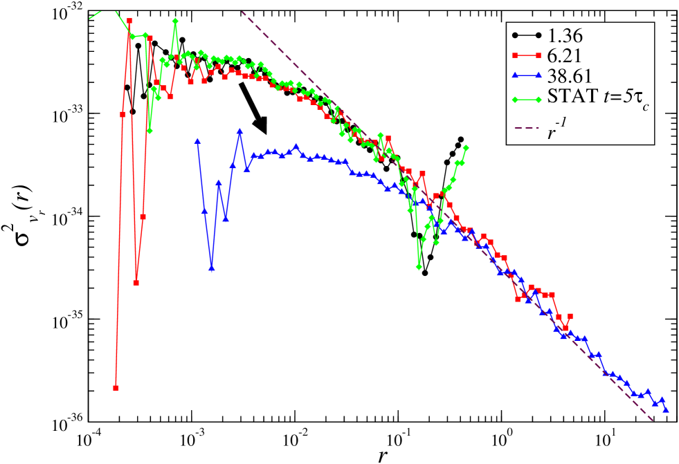
Figure 6: Radial velocity dispersion profile in physical coordinates at different scale factors $a$ (see labels) together with the profile for the STAT case. The arrow shows the direction of the density profile evolution in the cosmological case. A line with slope $r^{-1}$ (see Eq.5) is reported as reference.

Thus for $a>a_{LI}$ there is an energy injection into the system which causes an increase of the total energy: this occurs slowly enough that the system can rearrange its phase space configuration to satisfy the virial theorem (see the bottom panel of Fig.3). Therefore the energy increase corresponds to decrease of the kinetic energy: as $b\approx-1$ we have $\Delta E=-\Delta K_{p}$. Note the physical size of the structure increases almost simultaneously with the violation of the LI equation: this implies that the energy injection is spurious as otherwise the LI test should be verified.

The decrease of the kinetic energy corresponds to the fact that high velocity particles are slowed down. This is shown in Fig.7 (upper panel) where it is reported the evolution of the probability distribution function (PDF) $f(v)$ of the absolute value of the velocity. While for $a<a_{LI}$ we find that $f(v)$ remains almost stable, for $a>a_{LI}$ high velocity particles are slowed down and correspondingly the high velocity tail of $f(v)$ is significantly reduced. However the shape of $f(v)$ remains almost the same for $a>a_{LI}$. The failure of the LI test and consequent breakdown of the stable clustering regime is thus induced by the difficulty of integrating high velocity particles.

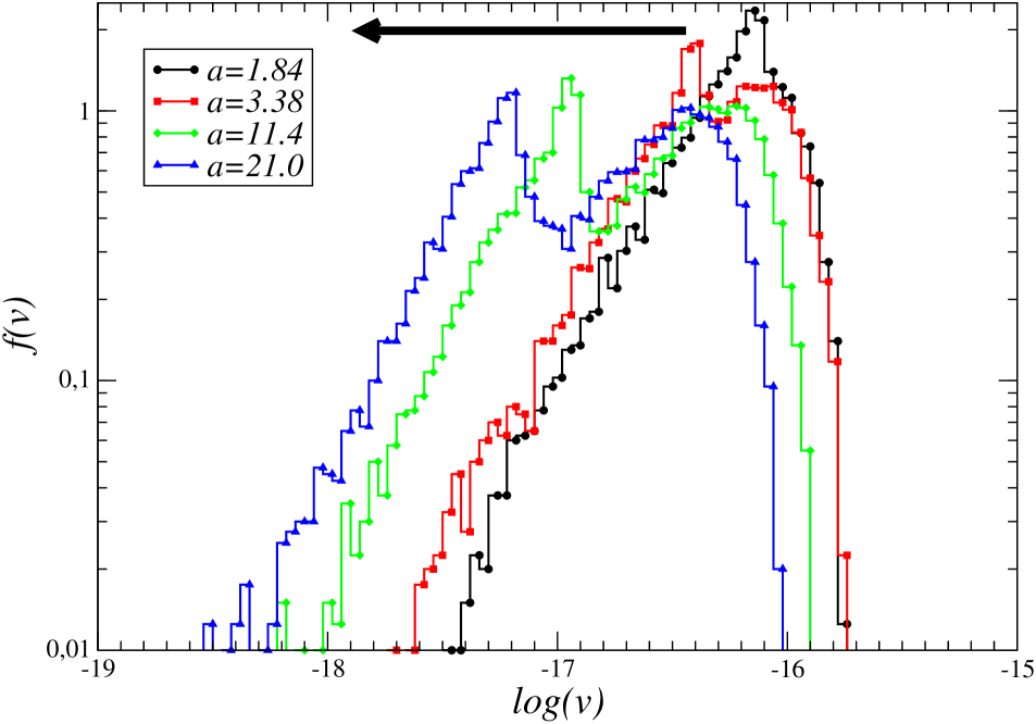
Figure 7: Evolution of the probability distribution function (PDF) of the absolute value of the velocity at different scale factors (see labels). The arrow shows the direction of the evolution.

High velocities are typically associated with close scatterings and the limited ability to resolve hard scattering between close neighbours, through which particles can increase their velocity, can also be traced by looking at the evolution of the nearest neighbour distribution $\omega(x)$ in comoving coordinates (see Fig.7): indeed, one may note that while for $a<a_{LI}$ $\omega(x)$ shows a peak that is shifted at smaller and smaller scale, corresponding to the fact that the structure is stable in physical coordinates, for $a>a_{LI}$ $\omega(x)$ does not change anymore reaching an “asymptotic” shape. This is a clear effect of the limited small scale resolution of the numerical code.

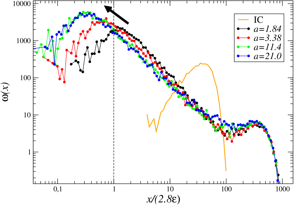
Figure 8: Evolution of the nearest neighbour distribution in comoving coordinates at different scale factors (see labels). The arrow shows the direction of the evolution. The initial distribution (IC) is also shown for comparison.

Finally we note that from the behaviours of the density profile and of the radial velocity dispersion, we can easily find that the pseudo phase-space density, for $a<a_{LI}$ and for $r>r_{c}$, scales as $\Phi(r)\sim r^{-5/2}$, i.e., the behaviour expected for the QEP (see Eq.6). On the other hand, for $a>a_{LI}$, at large radii, we find $\Phi(r)\sim r^{-3}\times r^{3/2}\sim r^{-1.5}$.

4.3 Summary

Let us summarise the situation in the two regimes that we have identified., i.e. $a<a_{LI}$ and $a>a_{LI}$.

1. For $a<a_{LI}$ the structure is in a QSS (i.e., $|W_{p}|\approx$ const.) and the density and velocity profiles are described by the collision-less equilibrium behaviours (Eqs.4-6). This situation corresponds to the stable clustering regime: the physical size and shape of the structure remains invariant during time evolution, modulo a marginal spatial extension of the power-law tail due to high velocity, but bounded, particles.

2. For $a>a_{LI}$ the structure is (almost) frozen in comoving coordinates and therefore its size in physical coordinates increases and its potential energy tends to zero as $W_{p}\propto-1/a$. The breakdown of the IL test marks a problem in the numerical integration of the particles equations of motion in this regime: this occurs because there is an injection of energy which causes the expansion of the structure in physical space. Correspondingly the density profile develops a $r^{-3}$ tail, approaching a NFW profile. The velocity dispersion profile still decays in a Keplerian way but with an amplitude that decreases with time equilibrating the smaller potential energy (in absolute value) of the structure, so that the virial ratio remains $b\approx-1$.

The decrease of the system kinetic energy for $a>a_{LI}$ corresponds to the fact that high velocity particles are slowed down and the PDF of the particles velocity $f(v)$ shifts toward smaller velocity values. This is indeed the consequence of the inaccurate integration of two-body collisions: it becomes more difficult to numerically resolve high velocity particles. As shown by the behaviour of the nearest neighbour distribution $\omega(x)$ these high velocity particles are also close neighbours. Indeed, $\omega(x)$ does not evolve anymore for $a>a_{LI}$, as it should if stable clustering were satisfied. We thus conclude that the inaccurate integration of hard collisions induces the change of regime at $a_{LI}$.

Note that $a_{LI}\approx 6$ corresponds to a time (see Eq.14) $(t_{break}-t_{0})/\tau_{c}\approx 50$ that is much smaller than the collisional relaxation time scale (see Eq.1) $\tau_{2}\approx 10^{4}\tau_{c}$ for a system with $N=10^{4}$ particles. This implies that the break-down of the QSS is not related to the expected evaporation due to two-body collisions for $t>\tau_{c}$.

Finally we note that the breakdown of the QSS, if physically originated, should not be associated with the breakdown of the LI test as we find. This shows that such a breakdown is induced by spurious reasons that we identify in the role of the inaccurate integration of high velocities particles and thus of hard scatterings. We will return on this important point in Sect.5.1.

5 Role of numerical integration parameters

In this section we study the effect of varying some of the most relevant numerical parameters that characterise the numerical integration: the softening length $\varepsilon$, the parameter that controls the time-stepping accuracy $\eta$, the opening angle $\theta$ of the tree algorithm and the accuracy of the relative cell-opening criterion $\phi$ .

5.1 Softening length

The softening length  has been varied in a range such that: (i) $\varepsilon<R_{0}$, i.e. it is smaller than the initial size of the structure so that the gravitational mean field force is well approximated at least at early times and (ii) the lower limit to $\varepsilon$ is due to numerical constraints: $\varepsilon>10^{-6}$ otherwise the integration time rapidly becomes too long and the simulation becomes unfeasible.

The potential energy in physical coordinates $W_{p}$ and the IL test (Fig.9) for simulations of the same system with $N=10^{4}$ particles and with different values of $\varepsilon$ (see Tab.1) — changed by a factor $10^{4}$ — show behaviours coherent with those discussed in Sect.4.2. Namely the two regimes found above, corresponding to $W_{p}\approx$ const. for $a<a_{LI}$ and $|W_{p}|\sim a^{-1}$ for $a>a_{LI}$, still characterise the temporal evolution. However, the transition between them depends on the softening length, i.e., $a_{LI}=a_{LI}(\varepsilon)$.

In particular, we find that $a_{LI}\approx 6$ for $\varepsilon\in[3.7\times 10^{-5},3.7\times 10^{-4}$], while outside this range $a_{LI}\approx 1$. This result is in agreement with Joyce & Sylos Labini (2013) who concluded that at most in that narrow range of $\varepsilon$ can the behaviour required, a QSS in the stable clustering regime, be reproduced by the N-body method.

Figure 9: Behaviour of $A(a)$ (Eq.26) for simulations with different $\varepsilon$ (see Tab.1 for details).

In order to understand the effect of a softening length which is too large with respect to the size of the structure, we have computed the gravitational potential energy of the structure with density profile described by Eq.3, in the case in which the pair potential is the GADGET one with different values $\varepsilon$. We find that the gravitational potential energy is very well approximated by the Newtonian value when $R(0.4)/(2\varepsilon)\approx 10$ and/or $R(0.8)/(2\varepsilon)\approx 100$, where $R(0.4)$ and $R(0.8)$ are the radii in comoving coordinates including respectively the 40% and 80% of the mass of the virialized structure.

The behaviours of $R(0.8)/(2\varepsilon)$ as a function of the expansion factor and for different values of the softening length are reported in Fig.10 (see the bottom panel). For $\varepsilon\geq 3.7\times 10^{-4}$ we have that $R(0.4)/(2.8\varepsilon)<10$: in this situation the effective mean field force due to all particles is different from Newtonian, i.e. the smoothening length is too large with respect to the size of the system. The effect of a too large softening thus corresponds to a deviation of the virial ratio from -1 (see the upper panel of Fig.10).

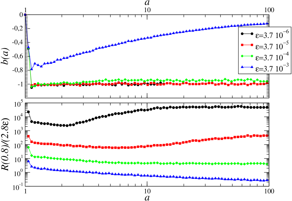
Figure 10: Upper panel: virial ratio as a function of the scale factor in simulations with different $\varepsilon$. Bottom panel: Length scale $R(0.8)$, including the $80\%$ of the mass of the virialized structure, normalised to $2.8\varepsilon$.

Instead, for $\varepsilon\leq 3.7\times 10^{-5}$ we find that, because the system remains stable in comoving coordinates $R(0.8)/(2.8\varepsilon)$ is larger than 100 for all values of the scale factor considered, and thus the virial ratio fluctuates around -1 at all times. Therefore we conclude that the relevant characteristic size of the structure remains large enough with respect to the force softening and that in this situation the Newtonian value of the mean field potential is well approximated by the smoothed potential.

The behaviour of the density profile is also coherent with what we have already found in Sect.4: for $a<a_{LI}$, the density profile obeys to Eq.3.

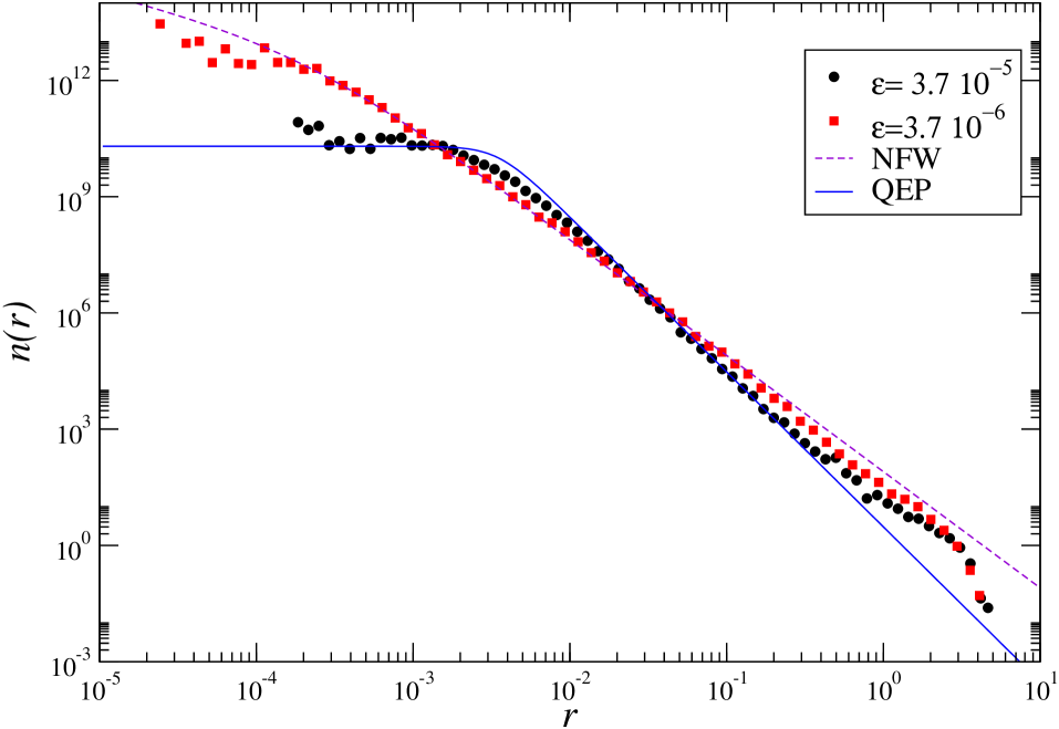
Figure 11: Density profile in physical coordinates at $a=4.6$ for the simulations M4a and M1a. The best fit with the NFW and QEP profiles are also reported.

Then, for $a>a_{LI}$, we observe a breaking of the stable clustering regime, and the density profile rapidly changes shape. In particular, it firstly deviates at small radii, displaying a power-law behaviour, and then at large ones where the slope tends to $-3$. The whole density profile can be fitted by a NFW behaviour (see Fig.11).

The evolution of the the velocity PDF $f(v)$ and the nearest neighbours distribution $\omega(x)$ for different values of $\varepsilon$ are coherent with the behaviours previously discussed. Namely, for large enough scale factors, i.e. $a\geq 10$, the simulation which behaves better according to the LI test (i.e., $\varepsilon=3.7\times 10^{-5}$) shows a more extended tail of $f(v)$ at high velocities than the others. This means a better ability of the code to follow high velocity particles. Correspondingly also $\omega(x)$ is peaked at smaller separations i.e. close particles can be better resolved for that value of the softening length. Both these facts point toward a better spatial (i.e., close neighbours) and temporal (i.e., high velocity particles) resolution when $\varepsilon=3.7\times 10^{-5}$.

Similarly to the behaviour of the density profile, whose small scale properties depend on $\varepsilon$ the nearest neighbour distribution and its peak shown an $\varepsilon$ dependence implying that the small scale properties of the system are determined by the spatial resolution used in the simulation.

5.2 Time-stepping accuracy

The accuracy of the time-stepping in the GADGET code is controlled by the parameter $\eta$: in particular, the time-stepping is fixed by

$$\Delta t=\sqrt{\frac{2\eta\varepsilon}{\mathcal{A}_{acc}}}\;,$$ (29)

where $\mathcal{A}_{acc}$ is the particle acceleration. It thus depends both on the softening length $\varepsilon$ and on the parameter $\eta$, i.e. the spatial and temporal resolution are strongly entangled. In order to determine the role of $\eta$ we consider a set of simulations in which all physical ($N,R_{0},b_{0}$) and numerical parameters ($\varepsilon$, $\theta$, $\phi$) are fixed and the time-stepping accuracy $\eta$ is varied by a factor $10^{2}$ (see Tab.1 for details).

From the LI test (see Fig.12) we find $a_{LI}=a_{LI}(\eta)$. Note that, as previously found, the LI test is verified in about the same range of scale factors where the potential energy is roughly constant and the structure is in the stable clustering regime.

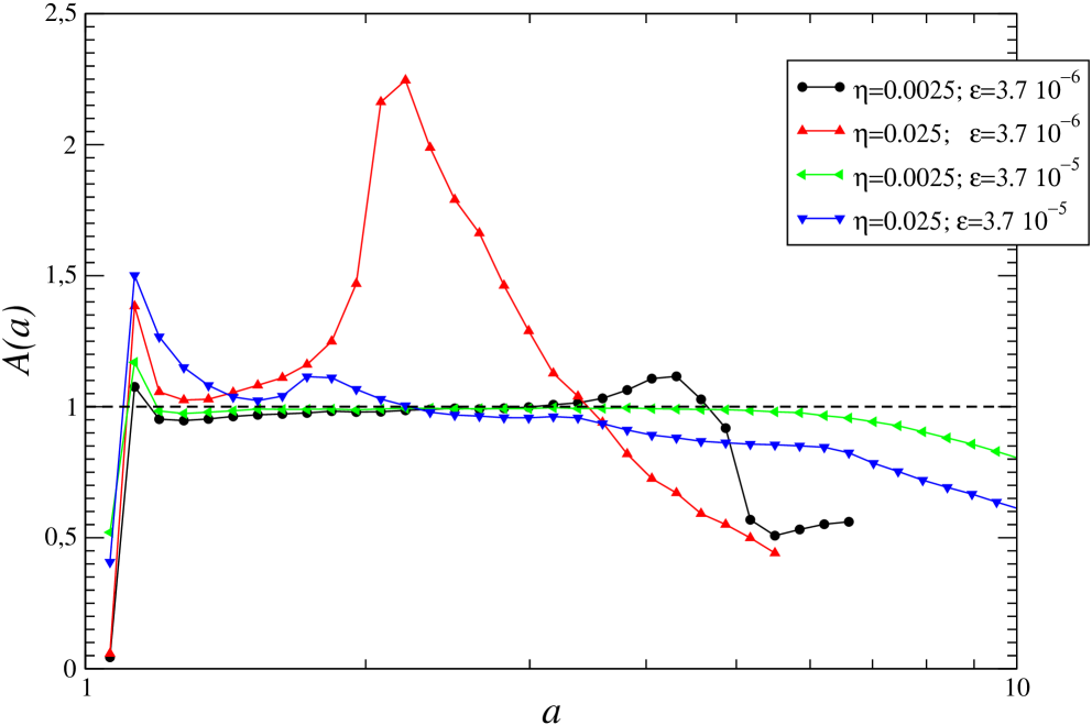
Figure 12: Behaviour of $A(a)$ (Eq.26) for simulations with different $\eta$ and $\varepsilon$ (see labels)

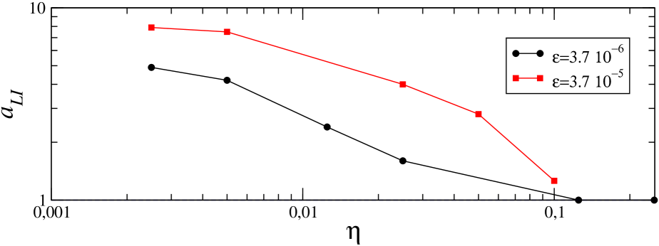
Figure 13: Behaviour of $a_{LI}$ as a function of $\eta$ for different values of the softening length $\varepsilon$.

The behaviour of $a_{LI}$ for different values of $\varepsilon$ and $\eta$ is reported in Fig.13: the larger is $\eta$ and the sooner occurs (i) the breakdown of the LI test, (ii) the departure from the stable clustering regime, (iii) the deviation from the QSS with the profile given by Eq.3. That is, at fixed $\varepsilon$, the larger is $\eta$ the smaller is $a_{LI}$. In agreement with the results discussed above, we find that the NFW profile provides a very good fit of the density profile for $a>a_{LI}$ (see Fig.14).

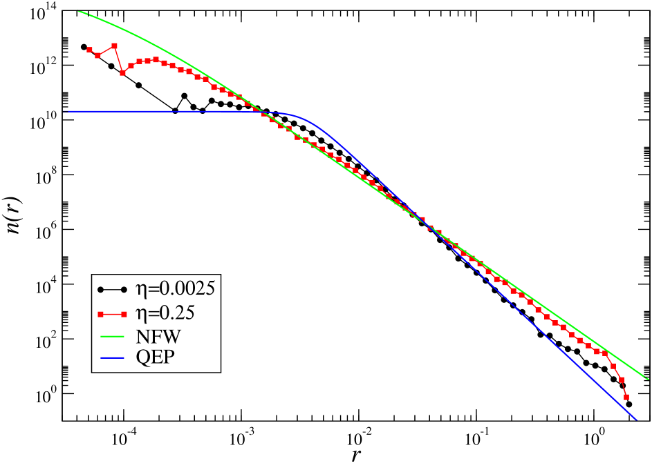
Figure 14: Density profile in physical coordinates at $a=2.5$ respectively for $\eta=0.0025$ and $\eta=0.25$. In both the cases the softening length is $\varepsilon=3.7\times 10^{-5}$.

The behaviours of the velocity $f(v)$ and of the nearest neighbours $\omega(x)$ distributions show that the smaller is $\eta$ and the better is the resolution of close neighbours and of high velocity particles. In addition, the high velocity tail of $f(v)$ is substantially reduced in the regime $a>a_{LI}$, in agreement with the results obtained by changing the softening length.

5.3 Other numerical parameters

Results obtained by varying the opening angle $\theta$ of the tree algorithm from 0.7 to 0.1 and the accuracy of the relative cell-opening criterion $\phi$, i.e. the parameter denominated ErrTolForceAcc, from $5\times 10^{-3}$ to $5\times 10^{-4}$ do not show sensible differences. This fact gives us reasonable confidence that the results we have presented are quite well converged with respect to these parameters.

5.4 Summary

The two main parameters that control the spatial and temporal resolution of the numerical integration, namely the softening length $\varepsilon$ and the time-stepping accuracy $\eta$, determine the range of time in which a simulation is well performing, i.e., the structure is a QSS and $W_{p}\approx$ const., the evolution is in agreement with stable clustering and the LI test is reasonably well satisfied. Thus the scale factor at which the breakdown of the LI test occurs is such that $a_{LI}=a_{LI}(\varepsilon,\eta)\;.$ We note that most of the discussion in the literature has focused the attention on the role of the softening length (see e.g. Splinter et al. (1988); Heitmann et al. (2005); Romeo et al. (2008); Joyce, Marcos & Baertschiger (2009); Power et al. (2003)): here we have found that a crucial parameter is also represented by the time-stepping accuracy.

Coherently with these results we found that the velocity PDF $f(v)$ and nearest neighbour distribution $\omega(x)$ depends on both the two parameters $\varepsilon$ and $\eta$. In particular the high velocity tail of $f(v)$ remains stable for $a<a_{LI}$ while there is a sensible deficit of high velocity particles for larger scale factors, due to the limited temporal resolution. Similarly $\omega(x)$ does not change anymore for $a>a_{LI}$, implying the departure from the stable clustering regime. In this situation the peak of $\omega(x)$ is determined by the values of both parameters $\varepsilon,\eta$.

In summary, tests performed by varying the softening parameter show that at fixed $\varepsilon<\ell$ the smaller is $\eta$ and the larger is $a_{LI}$. Our interpretation of this behaviour is that at a given level of numerical accuracy, determined by the choice of $\varepsilon,\eta$, hard scattering between particles can be resolved only up to a certain scale factor. Finally we note that the results of the evolution of the density profile are coherent with the ones found in Sect.4, namely for $a<a_{LI}$ this is well approximated by the QEP shape, while for $a>a_{LI}$ the profile shows the NFW behaviour.

We have discussed that there is an artificial injection of energy into the system during time evolution. We now conjecture that this is due to an inaccurate integration of two-body scatterings. When an hard scattering occurs the acceleration can be huge for a very short time interval $\delta\tau$: however if the time stepping is larger than $\delta\tau$ then the particle velocity will be overestimated by a large factor: this is a known numerical problem discussed in detail by, e.g., Knebe et al. (2000). Indeed, when $\eta$ decreases the amplitude of the time stepping (see Eq.29) gets shorter allowing a better sampling of the change of velocity during hard scatterings.

Instead, the change of particle velocity is $\Delta v=\Delta t\times\mathcal{A}_{acc}$ so that for hard scatterings $\mathcal{A}_{acc}\propto\varepsilon^{-2}$ we have $\Delta v\propto\sqrt{\eta/\varepsilon}$: the over-estimation of the velocity change increases when $\varepsilon$ gets smaller. Therefore we may conclude that the measured dependence of $a_{LI}$ on $\varepsilon,\eta$ and $N$ is coherent with the interpretation that there is a numerical problem in the integration of hard scatterings. Collisionality for the smaller softenings we use manifests itself most clearly in the breakdown of the LI test that represents a useful tool to study these effects.

It is interesting to note that collisional effects in cosmological simulations have been documented in previous studies by considering the comparison of different codes. In particular, Knebe et al. (2000) very explicitly demonstrates the effects of poor integration of hard two body collisions at small softenings. They showed that two-body scattering have effects which can be greatly amplified by inaccuracies of time integration and that the effects of such poorly integrated hard collisions is to lead to an artificial injection of energy into the system which causes an increasing its size. These results are indeed fully compatible with our results and interpretation (see also the discussion in Joyce & Sylos Labini (2013)).

6 Role of the physical parameters

In this section we first study the evolution of systems with same physical and numerical parameters but different particles number. That is, we discretize the system with a different number $N$ of particles taking fixed the total mass $M=m\times N$, with $m\propto 1/N$. Then we consider systems of different size $R_{0}$ but with the number of particles, their mass and the numerical parameters $[\varepsilon,\eta,\theta,\phi]$ fixed: this corresponds to change only the value of $\delta$ in Eq.12. Finally we change only the initial velocity dispersion and thus the initial virial ratio $b_{0}$.

6.1 Scaling with particles number

When the number of particles is small enough, i.e. $N<N^{*}\approx 10^{4}$ we observe that during the collapse phase the LI test always fails as $A(a)$ presents relatively large deviations from unity since $a\mathrel{\hbox to0.0pt{\lower 3.0pt\hbox{$\mathchar 536\relax$}\hss}\raise 2.0pt\hbox{$\mathchar 318\relax$}}1$ which persist at all times (see Fig.15). This can be interpreted as due to the fact that a few hard collisions occurring in the collapse phase substantially perturb the integration of the equation of motions. Note that according to the results obtained in Sect.5 the value of $N^{*}$ should in general depend on $\varepsilon,\eta$.

In simulations with $N>N^{*}\approx 10^{4}$ we find instead that $A(a)\approx 1$ soon after the collapse phase, with smaller fluctuations for larger $N$ values. The scale factor signing the break of the LI test weakly depends on $N$, i.e. $a_{LI}=a_{LI}(N)$: indeed it is found to be almost independent on $N$. This latter result seems surprising as from Eq.1 the collisional relaxation time should increase with $N$ so that one would naively expect that larger is $N$ and larger is $a_{LI}$.

To interpret this behaviour we recall that the density of the core after the collapse, $n_{c}$ in Eq.3, scales with the number of particles as $n_{c}\propto N^{2}$: at fixed mass density, by increasing the number of particles, the density of the core increases as $\rho_{c}=n_{c}\times m\propto N$, given that particles mass scales as $m\propto N^{-1}$ (Joyce, Marcos & Sylos Labini, 2009a). From Eq.1 we thus find that $\tau_{2}=\kappa N\tau_{c}\propto\kappa\sqrt{N}$, as $\tau_{c}\approx 1/\sqrt{G\rho_{c}}$. Given that $\kappa$ is weakly dependent on $N$, i.e. $\kappa\propto 1/\log(N)$, we thus find that $\tau_{2}$ is almost independent on $N$, at least for the limited range of $N$ we considered, i.e. $N=10^{4}\div 10^{5}$.

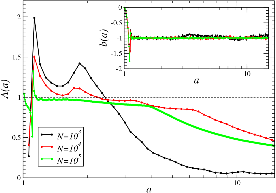
Figure 15: Behaviour of $A(a)$ (Eq.26) for simulations with different $N$ (see Tab.1) Insert panel: Behaviour of the virial ratio for the same simulations

In Fig.16 it is shown the density profile in physical coordinates for simulations with $N=10^{3},10^{5}$ particles: note that $n(r)$ has been normalised by recalling the results of Joyce, Marcos & Sylos Labini (2009a) where it was shown that the two parameters in Eq.3 scale as $r_{c}\approx N^{-1/3}$ and $n_{c}\approx N^{2}$. As we found in the previous sections, the breakdown of the stable clustering regime corresponds to a deformation of the profile.

Figure 16: Density profile in physical coordinates for simulations with $10^{3}$ and $10^{6}$ particles, at $a=4.9$, renormalised as explained in the text at different values of the expansion factor. The best fit with Eq.28 (NFW) and Eq.3 (QEP), respectively for $N=10^{3}$ and $N=10^{5}$ are reported as reference.

In the case shown in Fig.16, while for $N=10^{5}$ the simulation is still in the QSS regime, for the $N=10^{3}$ case the density profile is already well fitted by the NFW shape (see Fig.16).

6.2 Finite size effects

By considering the behaviours of the gravitational potential energy and of the LI test for simulations with different initial size $R_{0}$ we can conclude that $a_{LI}=a_{LI}(R_{0}).$ In particular, the smaller is $R_{0}$ and the smaller is $a_{LI}$.

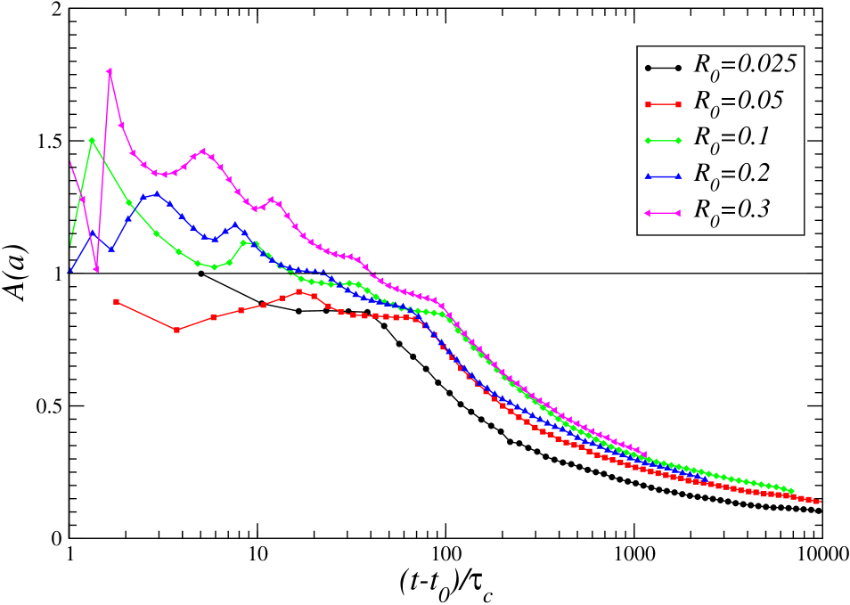
Figure 17: Behaviour of $A(a)$ (Eq.26) for simulations with different initial size $R_{0}$ as a function of time (normalised to $\tau_{c}(R_{0})$).

This fact can be simply interpreted by considering that when the system size decreases, the amplitude of the over-density $\delta=\delta(R_{0})$ increases and so the value of the characteristic time scale $\tau_{c}=\tau_{c}(R_{0})$ (see Tab.2). Thus, to compare the behaviours for different $R_{0}$ we plot (see Fig.17 — bottom panels) $W_{p}(a)$ and $A(a)$ as a function of time in units, for each value of $R_{0}$, of the corresponding value of $\tau_{c}=\tau_{c}(R_{0})$. The residual difference in the observed behaviours is due to the effect of the different ratio $R_{0}/L$: when $R_{0}>1/10L$ finite size corrections, i.e. the terms neglected in approximating Eq.7 with Eq.10 become important (Joyce & Sylos Labini, 2013).

The evolution of the density profile in physical coordinates for the systems with different $R_{0}$ (see Fig.18) shows that they firstly reach the QEP behaviour; then the density profile approaches the $r^{-3}$ behaviour, at different values of the scale factor for different $R_{0}$ and in a coherent way with the behaviour of $A(a)$.

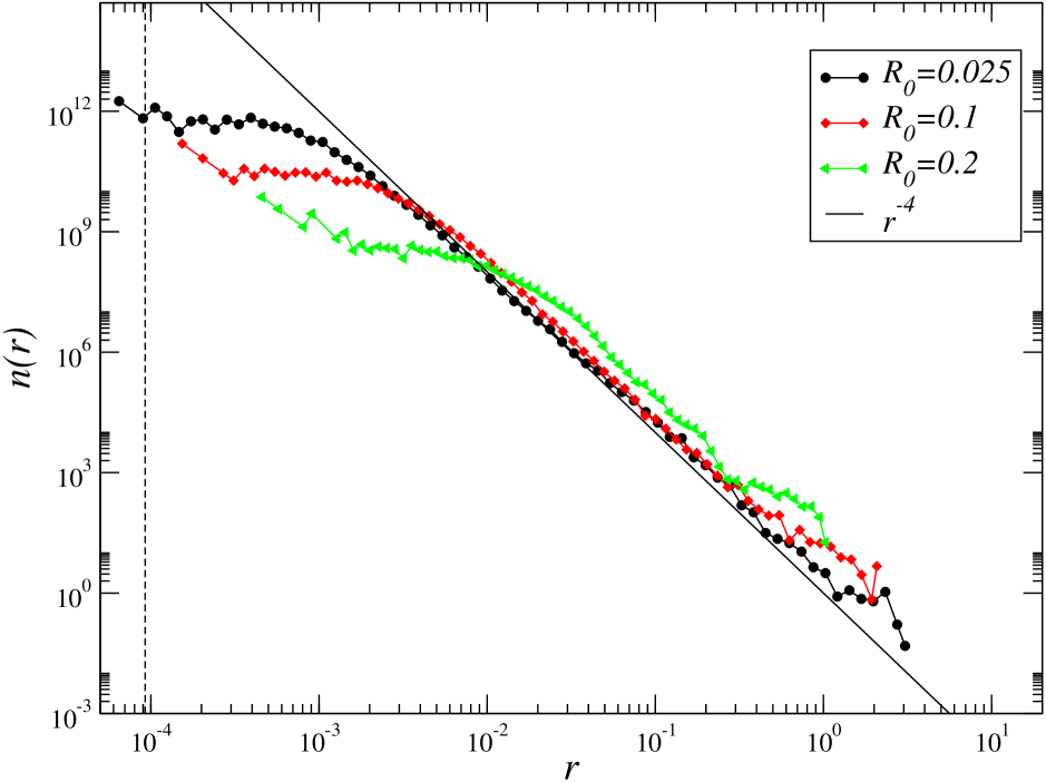
Figure 18: Density profile in physical coordinates at $a=2.5$ for different values of $R_{0}$ (see labels). The vertical dashed line correspond to $a\times\varepsilon$. A reference line with slope $-4$ is plotted as reference.

Finally we note that for long enough values of the scale factor the density profile for different $R_{0}$ converges precisely to the same behaviour characterised by a $x^{-3}$ decay. As discussed in Sect.5, at fixed time-stepping accuracy, the small scale properties of the distributions are determined by the value of the softening length. Indeed, independently on the initial value of $R_{0}$, for long enough times, all curves collapse on each other.

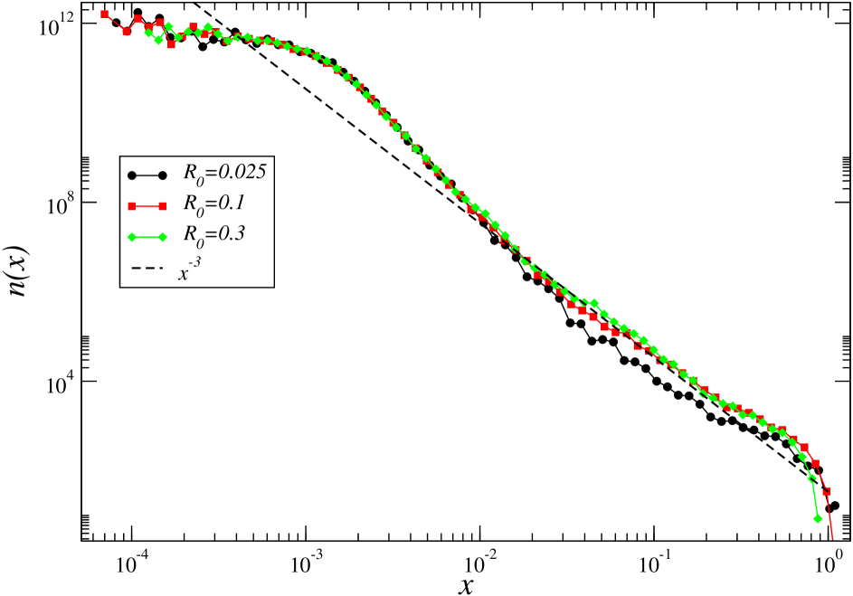
Figure 19: Density profile in comoving coordinates at $a=70$ for the simulations with $\varepsilon=3.7\times 10^{-4}$ and a different value of the initial radius $R_{0}$ (see labels). A reference line with slope $-4$ is plotted as reference.

6.3 Role of the initial velocity dispersion

The initial conditions we have considered can be thought to represent an halo which virializes in a relatively short time and which then evolve in isolation from the rest of the mass of the universe. Indeed, when $b_{0}\rightarrow-1$ the halo is already almost virialized while when $b_{0}\rightarrow 0$ the halo is far from such a configuration. However for $b_{0}\in[-1,0]$ the structure undergoes to a collapse, which can be less or more violent, that drives the system, in about the same time-scale $\tau_{c}$ (see Eq.2), into a virialized quasi-stationary state that can be well described as a collision-less equilibrium configuration (Sylos Labini, 2012).

Fig.20 shows the behaviour of $A(a)$ for simulations with different initial virial ratio $b_{0}\in[-1,0]$, i.e. with different initial velocity dispersion. We find that $a_{LI}=a_{LI}(b_{0})$: in particular, the smaller is $b_{0}$ the larger is $a_{LI}$. This behaviour is easily explained by considering that the closer the system is initially to the virial configuration and the less violent is the dynamics that drives the system into the virialized QSS (Sylos Labini, 2012): the larger is $b_{0}$ at the higher is the density of the core reached after the collapse.

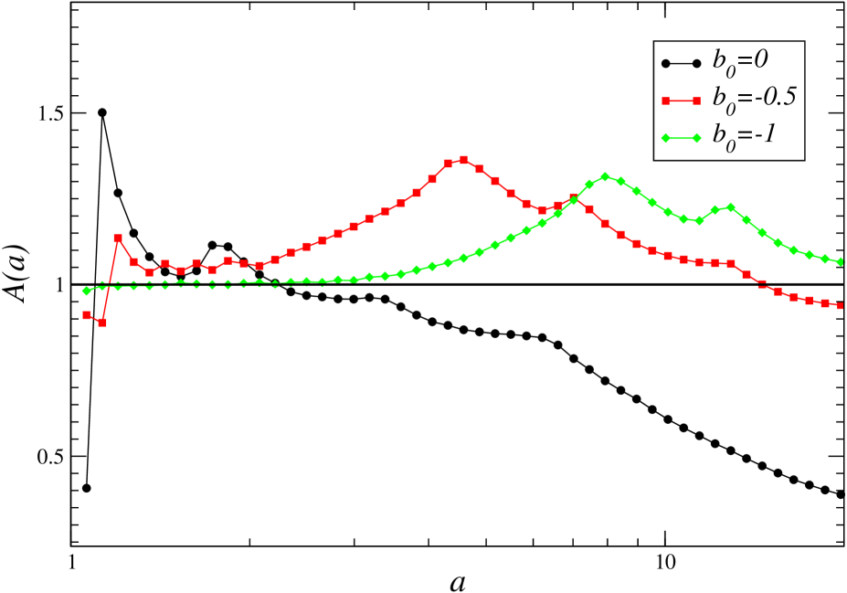
Figure 20: Behaviour of $A(a)$ (Eq.26) for for simulations with different initial size $b_{0}$.

We recall that, in the STAT case, the formation of the $r^{-4}$ is observed only when the collapse is violent enough that a fraction of the initial mass and energy is ejected from the system at the formation of the QSS: in Sylos Labini (2012) it was found that this occurs for $b_{0}>-1/2$. In this situation the system evolution is very similar to the $b_{0}=0$ case: at the beginning the density profile is well approximated by the QEP and then, for $a>a_{LI}$ it develops a $r^{-3}$ tail approaching the NFW shape also at small radii. Thus, although the $b_{0}=0$ is peculiar because the collapse is instantaneous in the continuous limit, it does not represent a pathological case and the $r^{-4}$ tail is formed as long as the collapse is violent enough that part of the mass and energy is ejected from the virialized structure.

For values of the initial virial ratio $b_{0}<-1/2$ the virialized structure after the collapse does not present a density profile with a $1/r^{4}$ tail. However for long enough times the density profile approaches the $1/r^{3}$ behaviour for any value of $b_{0}$. This shows that the $1/r^{3}$ is formed through the dynamical process and that it is thus independent on the initial conditions.

In Fig.21 it is shown the comparison of the density profile, in comoving coordinates, for simulations with different initial virial ratio and at different expansion factors: this confirms that the smaller is $b_{0}$ and the slower is the evolution. In particular, the smaller $b_{0}$ the longer it takes to form the $1/r^{3}$ tail, a behaviour that is approached at long enough times for any value of $b_{0}$.

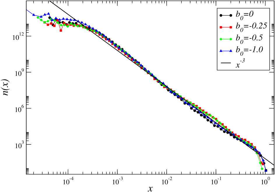
Figure 21: Comparison of the density profile in comoving coordinates for simulation with different initial virial ratio a $a=70$.

6.4 Summary

In summary we found that $a_{LI}=a_{LI}(R_{0},N,b_{0})$, i.e. the regime in which the system evolution is correctly numerically integrated depends on the physical parameters of the initial conditions.

For what concerns the dependence of $a_{LI}$ on $N$, we have noticed that: (i) for relatively small particles number, i.e. $N<N^{*}\approx 10^{4}$, the system never reaches the quasi-stationary state in the stable clustering regime. We have interpreted this behaviour as due the fact that a few hard scatterings are enough to perturb the macroscopic dynamics. (ii) On the other hand for large enough particles number, i.e., $N\in[10^{4},10^{5}]$, we find that the deviation from the QSS slowly depends on $N$. This occurs because when initial conditions are cold, the system contracts more for larger $N$ values, so that the virialized state has a core mass density $\rho_{c}\propto N$ and thus the typical time scale for crossing is $\tau_{c}\propto 1/\sqrt{N}$: in this situation the collisional time scale $\tau_{2}$ (see Eq.1) is very weakly dependent on $N$.

By decreasing the system size $R_{0}$ we find that $a_{LI}$ decreases as well: this is coherent with the fact that the smaller is $R_{0}$ and the smaller is the average distance between nearest neighbour particles in the core, and thus the higher the probability of hard collisions. However when we renormalize the behaviours to the proper characteristic time $\tau_{c}=\tau_{c}(R_{0})$ we find that the differences in the departure from the stable clustering regime become smaller: these residual differences are due to finite size effects.

In addition we have found that for long enough times all systems with initially different $R_{0}$ converge to the same density profile characterised by a $r^{-3}$ decay. This convergence is obtained because the numerical integration is badly performed, as shown by the LI test.

Finally, by increasing the initial velocity dispersion, the breakdown scale factor $a_{LI}$ is found to increase. This behaviour can be simply explained by considering that when $b_{0}\rightarrow 0$ the collapse is much more violent than for $b_{0}\rightarrow-1$; thus in the former case the core may reach higher densities sooner, then having a similar evolution to the cold case. In addition, when the initial velocity dispersion is high enough, the system remains in the stable clustering regime longer and until the softening length, that increases in physical coordinates, becomes large enough to perturb the evolution. At later times the system shows an evolution that is again similar to the cold case.

7 Discussion and Conclusion

In this paper we have tested a cosmological code (GADGET) by choosing very simple and idealised initial conditions. While we do not claim that this choice can be justified by any physical argument, i.e. the toy model does not represent any realistic physical system, we stress that in this way we have been able to make a series of controlled tests on the accuracy of a cosmological code. Given what we have learnt from this case, we discuss here some general ideas for the testing of a cosmological code in the case of more realistic initial conditions, as those predicted by standard models of galaxy formation. In order to consider separately these two different but, as we argue below, probably related issues, we first discuss the results of the simulations we have presented in this paper and then we briefly comment on the more complicated problem that requires more tests and work to be properly explored.

7.1 The control of the accuracy of a cosmological code: a toy model

The evolution of an isolated over-density in a cosmological N-body simulation is approximately equivalent, in physical coordinates, to the evolution of the same structure in an open system without expansion (Joyce & Sylos Labini, 2013). This equivalence is strictly verified in the limit of vanishing force smoothing and when the size of the over-density is much smaller than the size of the simulating box. When these conditions are satisfied, the evolution of the open system can be used as a template to compare the evolution in an expanding background with the aim of determining the accuracy of a cosmological simulation. The open system evolution is such that it relaxes to a virialized quasi stationary state (QSS) in a time $\tau_{c}$ (see Eq.2) (van Albada, 1982; Aarseth et al., 1988; Joyce, Marcos & Sylos Labini, 2009a; Sylos Labini, 2012) and it evaporates, due to collisional effects, in a time $\tau_{2}\gg\tau_{c}$ (see Eq.1). The QSS corresponds, in a cosmological N-body simulation, to an isolated structure in the stable clustering regime.

Joyce & Sylos Labini (2013) considered the evolution of an isolated over-density initially close to virial equilibrium: for this reason during the collapse its size and density vary a little. In this paper we considered a more general case, namely an isolated over-density with initial virial ratio in the range $b_{0}-\in[-1,0]$. When $b_{0}\rightarrow-1$ the initial conditions are warm enough that the collapse consists in a relatively small modification of system size. Instead when initial velocities are cold, i.e. $b_{0}\rightarrow 0$, the system largely contracts during the collapse, reducing considerably its size and shape and thus rapidly reaching, in its central core, a very high density (Sylos Labini, 2012).

Note that an initially cold, i.e. $b_{0}=0$, and spherical over-density does not represent a pathological case from the dynamical point of view: indeed, as firstly noticed by Stiavelli & Bertin (1987), a density profile with a $r^{-4}$ tail is a generic property of systems formed by a violent relaxation process. For instance, recently Sylos Labini (2012, 2013) found that this profile is formed also in the collapse of an initially spherical and isolated cloud of particles with a small enough velocity dispersion, with a uniform or power-law density profiles.

We found that, for $b_{0}\rightarrow 0$, once the system has reached a virialized configuration, its evolution can be characterised by two different regimes:

• (i) for scale factors $a<a_{LI}$ the potential energy in physical coordinates $W_{p}$ is approximately constant, the Layzer Irvine (LI) equation, describing the energy change in an expanding background, is well satisfied, the density profile is characterised by a $r^{-4}$ tail, characteristic of the quasi equilibrium profile (QEP) in the open case (see Eq.3), and the system is in the stable clustering regime, which means that it remains stable in physical coordinates.

• (ii) On the other hand for $a>a_{LI}$ we find that $|W_{p}|\sim a^{-1}$, there is a breakdown of the LI equation, the density profile becomes stable in comoving coordinates, which corresponds to the breakdown of the stable clustering regime, it develops a $r^{-3}$ tail and it can reasonably be fitted by the NFW profile.

In principle, the QSS has a lifetime $\tau_{2}$ that diverges with the number $N$ of system particles because of collisional effects. However we found that the time scale corresponding to $a_{LI}$ is (i) $t_{LI}<\tau_{2}$ and (ii) it depends on the numerical parameters of the simulation. Therefore this time scale is a numerical artifact: the relevant question is what determines it.

In order to answer to this question, we have performed various series of simulations by varying the integration parameters, such as the softening length of the gravitational force $\varepsilon$ (which, in the simulations we have performed, is fixed in comoving coordinates during the evolution) and the accuracy of the time-stepping $\eta$. We found that

$$a_{LI}=a_{LI}(\varepsilon,\eta).$$

In particular, we found that there is a narrow range of $\varepsilon$ (at fixed $\eta$) for which the simulation behaves “well” (i.e. regime (i) above). When $\varepsilon$ is much smaller than the initial inter-particle distance $\ell$ the integration is more difficult and $a_{LI}$ decreases: this fact can be interpreted as due the effect of hard collisions which require a high numerical accuracy to be correctly integrated. On the other hand, when $\varepsilon$ is of the order of the characteristic scale of the virialized system the mean field potential is no longer Newtonian so that the system deviates from the virialized configuration and from the quasi equilibrium profile.

That there is a problem in the accuracy of the numerical integration is confirmed by varying $\eta$ at fixed $\varepsilon$ (with $\varepsilon<\ell$): in particular when $\eta$ decreases $a_{LI}$ increases. This fact can be again interpreted in terms of a better accuracy of the numerical integration and in particular a more accurate integration of high velocity particles, which require a smaller time-stepping to be properly followed. Both tests by varying $\varepsilon$ and $\eta$ are thus consistent with the interpretation outlined above, that confirms the results by Joyce & Sylos Labini (2013): two-body scatterings perturb the accuracy of the simulation evolution. Thus the temporal and spatial resolution of the simulation are entangled and both must be considered for the determination of the optimal values of the numerical parameters.

Note that codes with adaptive spatial resolution (see e.g., Knebe et al. (2000); Teyssier (2001); Miniati & Colella (2007)) may perform much better than the fixed resolution case which we have considered in this paper. Indeed, it is clear such codes will, by construction, avoid respect. The tests we have discussed in this paper can be easily applied to other codes and a detailed study of codes with an adaptive mesh refinement is postponed to a forthcoming work.

Because of the violation of the LI, for $a>a_{LI}$, the system expands in physical coordinates, thus increasing its potential energy: this is due to an injection of energy into the system. From the tests performed by varying the softening length and the time-stepping parameter we conclude it is the effects of poor integrated hard two body collisions that leads to an artificial injection of energy into the system. This same conclusion was drawn by Knebe et al. (2000) by considering a comparison of different N-body codes. In summary we find, in agreement with Joyce & Sylos Labini (2013), that given a certain choice of numerical parameters, one may follow structure formation in the non linear regime, for a limited time which depends on several physical properties of the system. The results obtained here clearly show the role of the numerical (in)accuracy in the determination of the shape of the density profile structure.

In order to further test the result that the numerical integration becomes inaccurate because of collisional effects, we have, at fixed numerical parameters, changed the physical parameters of the initial conditions. Namely we have varied the number of particles $N$ (at fixed density), the size of the structure $R_{0}$ and the initial velocity dispersion (and thus the initial virial ratio $b_{0}$). As result we found that

$$a_{LI}=a_{LI}(N,R_{0},b_{0})\;.$$

When decreasing $R_{0}$ we find that $a_{LI}$ decreases: the initial inter-particle distance gets smaller, as $\ell\propto R_{0}$, and thus hard scatterings are more probable. The dependence of $a_{LI}$ on the particle number clearly shows the effect of two-body collisions. For small particle number, i.e. $N<10^{4}$, the system never reaches a QSS and the LI test fails at all times. We then find that, at fixed $\varepsilon$ and $\eta$, and for $N\in[10^{4},10^{5}]$ the breakdown expansion factor $a_{LI}$ is almost independent with $N$. This behaviour can be interpreted as due to the fact that the larger is $N$, the larger the core mass density and thus the characteristic time $\tau_{c}$: in this situation the collisional time scale $\tau_{2}$ in Eq.1 becomes almost independent on $N$.

Finally by increasing the initial velocity dispersion, i.e. decreasing $b_{0}$, we find that $a_{LI}$ increases: indeed, as shown in Sylos Labini (2012), when the initial configuration is closer to the virial equilibrium, i.e. $b_{0}=-1$, the collapse is less violent so that the size and density of the structure after the collapse are not largely changed as it occurs when $b_{0}=0$. In this latter case the core of the structure after the collapse may reach very high densities, i.e. a more favourable condition for the occurrence of two-body scatterings. However, we have found that for $b_{0}\in[-1,0]$ the density profile, in the long time evolution, approaches the same NFW shape. Thus, the density profile, for long enough times, approaches the $1/r^{3}$ behaviour for any value of $b_{0}$ a fact that shows that this tail is formed by the same dynamics process, independent on the initial conditions, in all cases.

While the origin of the $r^{-4}$ can be understood by considering that the energy of particles orbiting around the core is conserved Sylos Labini (2012), the effect of inaccurately integrated two-body scatterings is indeed that of perturbing such energy conservation. The energy injection, is especially efficient for the fastest particles, i.e. those that form the tail of the density profile. A quantitative study of this effect is postponed to a forthcoming work, but qualitatively we may conclude that the deformation of the density profile is related to the inability to resolve numerically high velocity particles and thus to conserve their energy properly.

7.2 Some comments on more complex initial conditions

The simplicity of the system considered as initial conditions has let us to develop systematic tests to control the accuracy of a cosmological code. The principal result that we have obtained is that the range of redshifts where the numerical integration of a certain structure is reliable, i.e. it follows the stable clustering regime and it passes the LI test, is in general limited to narrow one that is dependent on the various physical (number of particles, velocity dispersion, density and amplitude of the over-density) and numerical (softening length, time-stepping) parameters of a given simulation. Therefore, our results suggest that the limited numerical resolution of a given simulation can be not sufficient to integrate the formation of structures with a wide range in size and mass as those formed in the currently favoured cosmological models structures through a hierarchical aggregation. A more detailed study of the more complex cosmological case is thus required.

Here we note that, if one is not able to integrate correctly the evolution of this simplified system, one will encounter more difficult problems if one wants to properly simulate the formation of structures of different sizes, with different particle numbers and in a complex environment as that occurring in the case of typical initial conditions of structure formation models. On the other hand the choice of the physical and numerical parameters adopted in this paper could be completely unrealistic and thus irrelevant for the case of a cosmological simulations that uses initial conditions as those predicted by standard models of galaxy formation.

In this respect, we note that the numerical parameters have been varied in a relatively large range, i.e. $\varepsilon\in[10^{-6},10^{-3}]$ and $\eta\in 2.5\times[10^{-3},10^{-1}]$. In addition, the number of particles used, ranging in $N\in[10^{3},10^{5}]$, is comparable to the number of particles which form a single halo in a typical cosmological simulation (Springel et al., 2005). Thus the system we considered, once it reaches a virialized state, can be though to represent a simplified toy model approximating a virialized cosmological halo at its formation time. This structure, however then evolves as if it were isolated from the rest of the universe. Thus, such a self-gravitating system presents several differences with respect to the halos formed in typical cosmological simulations: it is spherical and isolated so that it has initially a simple geometry, it is not subjected neither to mass accretion nor to tidal interactions with the neighbouring structures, it does not fragment into (macroscopic) substructures during its evolution and it does not collide with structures of comparable size.

A possible method to control both the role of the physical and the numerical parameters in a more complex cosmological simulations was presented in Joyce & Sylos Labini (2013), where it was outlined a sort of recipe that can be simply implemented and that can furnish a general manner for testing the accuracy of a simulation of halos containing $N$ particles. This is simply based on the testing of whether an halo formed in a complex environment, once it is isolated, evolves in agreement with stable clustering and represents a quasi-stationary configuration, given the same numerical parameter of the numerical integration (softening length, time-stepping, etc.) and the same physical parameters of the structure (number of particles, size and velocity dispersion). The implementation of this test is postponed to a forthcoming work.

As a final remark, we stress that we have observed that the density profile of the virialized structure formed from the simple initial conditions we have considered converges, for a wide range the numerical and physical parameters of the simulation, to the NFW profile, i.e. the same profile observed in cosmological N-body simulations that start from the typical initial conditions predicted by standard models of galaxy formation. Whether this is a coincidence or whether also standard cosmological halos are seriously affected by the numerical (in)accuracy of the numerical integration is an open problem that will explored in full details in forthcoming works

I thank Michael Joyce for useful discussions and comments, Roberto Ammendola and Nazario Tantalo for the valuable assistance in the use of the Fermi supercomputer where the simulations have been performed. I also would like to thank Alessandro Romeo for a number of very useful comments and suggestions that have allowed to improve the presentation of the paper.

References

- Aarseth et al. (1988) Aarseth S., Lin D., Papaloizou J., 1988, Astrophys. J., 324, 288
- Aarseth (2003) Aarseth S. J., 2003,Gravitational N-Body Simulations: Tools and Algorithms, Cambridge University Press
- Bertin (2000) Bertin G., 2000, Dynamics of Galaxies, Cambridge University Press
- Boily & Athanassoula (2006) Boily C., Athanassoula E., 2006, Mon. Not. R. Astr. Soc., 369, 608
- Chandrasekhar (1943) Chandrasekhar S., 1943, Rev. Mod. Phys., 15, 1
- David & Theuns (1989) David M., Theuns T., 1989, Mon. Not. R. Astr. Soc., 240, 957
- Diemand et al. (2004) Diemand J., Moore B., Stadel J., Kazantzidis S., 2004, Mon. Not. R. Astron. Soc., p. 977
- Gabrielli et al. (2006) Gabrielli A., Baertschiger T., Joyce M., Marcos B., Sylos Labini F., 2006, Phys. Rev., E74, 021110
- Gabrielli et al. (2010) Gabrielli A., Joyce M., Marcos B., 2010, Phys. Rev. Lett., 105, 210602
- Heggie & Hut (2003) Heggie D., Hut P., 2003, The Gravitational Million-Body Problem: A Multidisciplinary Approach to Star Cluster Dynamics. Cambridge
- Hénon (1964) Hénon M., 1964, Ann. Astrophys., 27, 1
- Heitmann et al. (2005) Heitmann K., Ricker P. M., Warren M. S., Habib S., 2005, Astrophy. J. Supp, 160, 28
- Knebe, Green & Benney (2003) Knebe A., Green A., Binney J, 2001, Mon.Not.Roy.Astron.Soc., 325, 845
- Knebe et al. (2000) Knebe A., Kravtsov A.V., Gottlober S., Klypin, A.A., 2000 Mon.Not.Roy.Astron.Soc., 317, 630
- Iannuzzi & Dolag (2011) Iannuzzi F., Dolag K., 2011, Mon.Not.Roy.Astron.Soc., 417, 2846
- Joyce, Marcos & Baertschiger (2009) Joyce M., Marcos B., Baertschiger T., 2009, Mon. Not. R. Astr. Soc., 394, 751
- Joyce, Marcos & Sylos Labini (2009a) Joyce M., Marcos B., Sylos Labini F., 2009, Mon. Not. R. Astr. Soc., 397, 775
- Joyce, Marcos & Sylos Labini (2009b) Joyce M., Marcos B., Sylos Labini F., 2009, Journal of Statistical Mechanics, P04019