Classification of Stochastic Runge–Kutta Methods for the Weak Approximation of Stochastic Differential Equations

Abstract

In the present paper, a class of stochastic Runge–Kutta methods containing the second order stochastic Runge–Kutta scheme due to E. Platen for the weak approximation of Itô stochastic differential equation systems with a multi–dimensional Wiener process is considered. Order one and order two conditions for the coefficients of explicit stochastic Runge–Kutta methods are solved and the solution space of the possible coefficients is analyzed. A full classification of the coefficients for such stochastic Runge–Kutta schemes of order one and two with minimal stage numbers is calculated. Further, within the considered class of stochastic Runge–Kutta schemes coefficients for optimal schemes in the sense that additionally some higher order conditions are fulfilled are presented.

and

1 Introduction

Recently, the development of numerical schemes for strong as well as weak approximation of stochastic differential equations (SDEs) has focused amongst others on Runge–Kutta type schemes [1, 2, 5, 6, 7, 8, 9, 10, 11, 12, 13]. This is due to the increasing complexity of stochastic Taylor expansions and the desire to avoid derivatives in higher order approximation schemes. In section 2, a class of stochastic Runge–Kutta (SRK) methods due to Rößler [10, 11, 12] for the weak approximation of Itô SDE systems with a multi–dimensional Wiener process is considered. This class contains as a special case the second order SRK scheme proposed by Platen [5] as well as the class of SRK methods proposed by Tocino and Vigo-Aguiar [13]. Order conditions for coefficients of the SRK methods have been calculated by applying the multi-colored rooted tree analysis due to Rößler [10, 11, 12]. In contrast to earlier work on this topic, the aim of the present paper is to analyze these order conditions with the objective to determine a full classification of the coefficients for this class of SRK methods. A full classification for order one SRK schemes with $s=1$ stage and for order one SRK schemes with deterministic order two for $s=2$ stages as well as for second order SRK schemes with $s=3$ stages is calculated in section 3. Further, some optimal schemes are derived from this classification in section 4 by taking into account additional higher order conditions. Their performance is studied by some numerical examples in section 5.

We denote by $(X_{t})_{t\in I}$ the solution of the $d$-dimensional Itô SDE defined by

$${\mathrm{d}}X_{t}=a(t,X_{t})\,{\mathrm{d}}t+b(t,X_{t})\,{\mathrm{d}}W_{t},\qquad X_{t_{0}}=x_{0},$$ (1)

with an $m$-dimensional Wiener process $(W_{t})_{t\geq 0}$ and $I=[t_{0},T]$. We assume that the Borel-measurable coefficients $a:I\times\mathbb{R}^{d}\rightarrow\mathbb{R}^{d}$ and $b:I\times\mathbb{R}^{d}\rightarrow\mathbb{R}^{d\times m}$ satisfy a Lipschitz and a linear growth condition such that the Existence and Uniqueness Theorem [5] applies. In the following, let $b^{j}(t,x)=(b^{i,j}(t,x))_{1\leq i\leq d}\in\mathbb{R}^{d}$ denote the $j$th column of the diffusion matrix $b(t,x)$ for $j=1,\ldots,m$.

Let a discretization $I_{h}=\{t_{0},t_{1},\ldots,t_{N}\}$ with $t_{0}<t_{1}<\ldots<t_{N}=T$ of the time interval $I=[t_{0},T]$ with step sizes $h_{n}=t_{n+1}-t_{n}$ for $n=0,1,\ldots,N-1$ be given. Further, define $h=\max_{0\leq n<N}h_{n}$ as the maximum step size. Let $C_{P}^{l}(\mathbb{R}^{d},\mathbb{R})$ denote the space of all $g\in C^{l}(\mathbb{R}^{d},\mathbb{R})$ fulfilling a polynomial growth condition and let $g\in C_{P}^{k,l}(I\times\mathbb{R}^{d},\mathbb{R})$ if $g(\cdot,x)\in C^{k}(I,\mathbb{R})$ and $g(t,\cdot)\in C_{P}^{l}(\mathbb{R}^{d},\mathbb{R})$ for all $t\in I$ and $x\in\mathbb{R}^{d}$ [5].

Definition 1.1

A time discrete approximation $Y=(Y_{t})_{t\in I_{h}}$ converges weakly with order $p$ to $X$ as $h\rightarrow 0$ at time $t\in I_{h}$ if for each $f\in C_{P}^{2(p+1)}(\mathbb{R}^{d},\mathbb{R})$ exist a constant $C_{f}$ and a finite $\delta_{0}>0$ such that

$$|\operatorname{E}(f(X_{t}))-\operatorname{E}(f(Y_{t}))|\leq C_{f}\,h^{p}$$ (2)

holds for each $h\in\,]0,\delta_{0}[\,$.

2 Stochastic Runge–Kutta Methods

We consider stochastic Runge–Kutta methods as proposed in [10, 11, 12] for the weak approximation of SDE (1). Therefore, the $d$-dimensional approximation process $Y$ of an explicit $s$-stage SRK method is defined by $Y_{t_{0}}=x_{0}$ and

$$\begin{split}Y_{t_{n+1}}=Y_{t_{n}}&+\sum_{i=1}^{s}\alpha_{i}\,a(t_{n}+c_{i}^{(0)}h_{n},H_{i}^{(0)})\,h_{n}\\ &+\sum_{i=1}^{s}\sum_{k=1}^{m}\beta_{i}^{(1)}\,b^{k}(t_{n}+c_{i}^{(1)}h_{n},H_{i}^{(k)})\,\hat{I}_{(k)}\\ &+\sum_{i=1}^{s}\sum_{k=1}^{m}\beta_{i}^{(2)}\,b^{k}(t_{n}+c_{i}^{(1)}h_{n},H_{i}^{(k)})\,\tfrac{\hat{I}_{(k,k)}}{\sqrt{h_{n}}}\\ &+\sum_{i=1}^{s}\sum_{\begin{subarray}{c}k,l=1\\ k\neq l\end{subarray}}^{m}\beta_{i}^{(3)}\,b^{k}(t_{n}+c_{i}^{(2)}h_{n},\hat{H}_{i}^{(l)})\,\hat{I}_{(k)}\\ &+\sum_{i=1}^{s}\sum_{\begin{subarray}{c}k,l=1\\ k\neq l\end{subarray}}^{m}\beta_{i}^{(4)}\,b^{k}(t_{n}+c_{i}^{(2)}h_{n},\hat{H}_{i}^{(l)})\,\tfrac{\hat{I}_{(k,l)}}{\sqrt{h_{n}}}\end{split}$$ (3)

for $n=0,1,\ldots,N-1$ with stage values

$$H_{i}^{(0)} = \,\,Y_{t_{n}} +\sum_{j=1}^{i-1}A_{ij}^{(0)}\,a(t_{n}+c_{j}^{(0)}h_{n},H_{j}^{(0)})\,h_{n}$$

$$+\sum_{j=1}^{i-1}\sum_{r=1}^{m}B_{ij}^{(0)}\,b^{r}(t_{n}+c_{j}^{(1)}h_{n},H_{j}^{(r)})\,\hat{I}_{(r)}$$

$$H_{i}^{(k)} = \,\,Y_{t_{n}} +\sum_{j=1}^{i-1}A_{ij}^{(1)}\,a(t_{n}+c_{j}^{(0)}h_{n},H_{j}^{(0)})\,h_{n}$$

$$+\sum_{j=1}^{i-1}B_{ij}^{(1)}\,b^{k}(t_{n}+c_{j}^{(1)}h_{n},H_{j}^{(k)})\,\sqrt{h_{n}}$$

$$\hat{H}_{i}^{(k)} = \,\,Y_{t_{n}} +\sum_{j=1}^{i-1}A_{ij}^{(2)}\,a(t_{n}+c_{j}^{(0)}h_{n},H_{j}^{(0)})\,h_{n}$$

$$+\sum_{j=1}^{i-1}B_{ij}^{(2)}\,b^{k}(t_{n}+c_{j}^{(1)}h_{n},H_{j}^{(k)})\,\sqrt{h_{n}}$$

for $i=1,\ldots,s$ and $k=1,\ldots,m$. Here, $\alpha,\beta^{(1)},\dots,\beta^{(4)},c^{(q)}\in\mathbb{R}^{s}$ and $A^{(q)}$, $B^{(q)}\in\mathbb{R}^{s\times s}$ for $0\leq q\leq 2$ with $A_{ij}^{(q)}=B_{ij}^{(q)}=0$ for $j\geq i$ are the vectors and matrices of coefficients of the SRK method. We choose $c^{(q)}=A^{(q)}e$ for $0\leq q\leq 2$ with a vector $e=(1,\ldots,1)^{T}$ [10]. In the following, the product of column vectors is defined component-wise. The coefficients of the SRK method (3) are determined by the following Butcher tableau:

$c^{(0)}$	${A}^{(0)}$	$B^{(0)}$
$c^{(1)}$	${A}^{(1)}$	$B^{(1)}$
$c^{(2)}$	${A}^{(2)}$	$B^{(2)}$
	$\alpha^{T}$	${\beta^{(1)}}^{T}$	${\beta^{(2)}}^{T}$
		${\beta^{(3)}}^{T}$	${\beta^{(4)}}^{T}$

The random variables of the SRK method are defined by three-point distributed random variables with $\operatorname{P}(\hat{I}_{(r)}=\pm\sqrt{3\,h_{n}})=\frac{1}{6}$ and $\operatorname{P}(\hat{I}_{(r)}=0)=\frac{2}{3}$. Further, $\hat{I}_{(k,l)}=\frac{1}{2}(\hat{I}_{(k)}\,\hat{I}_{(l)}+V^{k,l})$. The $V^{k,l}$ are independent two-point distributed random variables with $\operatorname{P}(V^{k,l}=\pm h_{n})=\frac{1}{2}$ for $l=1,\ldots,k-1$, $V^{k,k}=-h_{n}$ and $V^{k,l}=-V^{l,k}$ for $l=k+1,\ldots,m$ and $k=1,\ldots,m$ [5].

By the application of the multi–colored rooted tree analysis [10, 12], order conditions for the coefficients of the SRK method (3) can be easily determined. As a result of this, the following Theorem 2.1 due to Rößler [12] gives order conditions for the SRK method (3) up to order two.

Theorem 2.1

Let $a^{i},b^{ij}\in C_{P}^{2,4}(I\times\mathbb{R}^{d},\mathbb{R})$ for $1\leq i\leq d$, $1\leq j\leq m$. If the coefficients of the SRK method (3) fulfill the equations

$$1 .\quad\alpha^{T}e=1\qquad\qquad 2.\quad {\beta^{(4)}}^{T}e=0\qquad\qquad 3.\quad {\beta^{(3)}}^{T}e=0$$

$$4 .\quad({\beta^{(1)}}^{T}e)^{2}=1\qquad\qquad 5.\quad {\beta^{(2)}}^{T}e=0\qquad\qquad 6.\quad {\beta^{(1)}}^{T}{B^{(1)}}e=0$$

$$7 .\quad{\beta^{(3)}}^{T}{B^{(2)}}e=0$$

then the SRK method converges with order 1 in the weak sense. In addition, if $a^{i},b^{ij}\in C_{P}^{3,6}(I\times\mathbb{R}^{d},\mathbb{R})$ for $1\leq i\leq d$, $1\leq j\leq m$ and if the equations

$$8 .\quad\alpha^{T}A^{(0)}e=\tfrac{1}{2}\qquad\qquad 9.\quad \alpha^{T}(B^{(0)}e)^{2}=\tfrac{1}{2}$$

$$10 .\quad({\beta^{(1)}}^{T}e)(\alpha^{T}B^{(0)}e)=\tfrac{1}{2}\qquad\qquad 11.\quad ({\beta^{(1)}}^{T}e)({\beta^{(1)}}^{T}A^{(1)}e)=\tfrac{1}{2}$$

$$12 .\quad{\beta^{(3)}}^{T}A^{(2)}e=0\qquad\qquad 13.\quad {\beta^{(2)}}^{T}B^{(1)}e=1$$

$$14 .\quad{\beta^{(4)}}^{T}B^{(2)}e=1\qquad\qquad 15.\quad ({\beta^{(1)}}^{T}e)({\beta^{(1)}}^{T}(B^{(1)}e)^{2})=\tfrac{1}{2}$$

$$16 .\quad({\beta^{(1)}}^{T}e)({\beta^{(3)}}^{T}(B^{(2)}e)^{2})=\tfrac{1}{2}\qquad 17.\quad {\beta^{(1)}}^{T}(B^{(1)}(B^{(1)}e))=0$$

$$18 .\quad{\beta^{(3)}}^{T}(B^{(2)}(B^{(1)}e))=0\qquad 19.\quad {\beta^{(3)}}^{T}(A^{(2)}(B^{(0)}e))=0$$

$$20 .\quad{\beta^{(1)}}^{T}(A^{(1)}(B^{(0)}e))=0\qquad 21.\quad \alpha^{T}(B^{(0)}(B^{(1)}e))=0$$

$$22 .\quad{\beta^{(2)}}^{T}A^{(1)}e=0\qquad 23.\quad {\beta^{(4)}}^{T}A^{(2)}e=0$$

$$24 .\quad{\beta^{(1)}}^{T}((A^{(1)}e)(B^{(1)}e))=0\qquad 25.\quad {\beta^{(3)}}^{T}((A^{(2)}e)(B^{(2)}e))=0$$

$$26 .\quad{\beta^{(4)}}^{T}(A^{(2)}(B^{(0)}e))=0\qquad 27.\quad {\beta^{(2)}}^{T}(A^{(1)}(B^{(0)}e))=0$$

$$28 .\quad{\beta^{(2)}}^{T}(A^{(1)}(B^{(0)}e)^{2})=0\qquad 29.\quad {\beta^{(4)}}^{T}(A^{(2)}(B^{(0)}e)^{2})=0$$

$$30 .\quad{\beta^{(3)}}^{T}(B^{(2)}(A^{(1)}e))=0\qquad 31.\quad {\beta^{(1)}}^{T}(B^{(1)}(A^{(1)}e))=0$$

$$32 .\quad{\beta^{(2)}}^{T}(B^{(1)}e)^{2}=0\qquad 33.\quad {\beta^{(4)}}^{T}(B^{(2)}e)^{2}=0$$

$$34 .\quad{\beta^{(4)}}^{T}(B^{(2)}(B^{(1)}e))=0\qquad 35.\quad {\beta^{(2)}}^{T}(B^{(1)}(B^{(1)}e))=0$$

$$36 .\quad{\beta^{(1)}}^{T}(B^{(1)}e)^{3}=0\qquad 37.\quad {\beta^{(3)}}^{T}(B^{(2)}e)^{3}=0$$

$$38 .\quad{\beta^{(1)}}^{T}(B^{(1)}(B^{(1)}e)^{2})=0\qquad 39.\quad {\beta^{(3)}}^{T}(B^{(2)}(B^{(1)}e)^{2})=0$$

$$40 .\quad\alpha^{T}((B^{(0)}e)(B^{(0)}(B^{(1)}e)))=0$$

$$41 .\quad{\beta^{(1)}}^{T}((A^{(1)}(B^{(0)}e))(B^{(1)}e))=0$$

$$42 .\quad{\beta^{(3)}}^{T}((A^{(2)}(B^{(0)}e))(B^{(2)}e))=0$$

$$43 .\quad{\beta^{(1)}}^{T}(A^{(1)}(B^{(0)}(B^{(1)}e)))=0$$

$$44 .\quad{\beta^{(3)}}^{T}(A^{(2)}(B^{(0)}(B^{(1)}e)))=0$$

$$45 .\quad{\beta^{(1)}}^{T}(B^{(1)}(A^{(1)}(B^{(0)}e)))=0$$

$$46 .\quad{\beta^{(3)}}^{T}(B^{(2)}(A^{(1)}(B^{(0)}e)))=0$$

$$47 .\quad{\beta^{(1)}}^{T}((B^{(1)}e)(B^{(1)}(B^{(1)}e)))=0$$

$$48 .\quad{\beta^{(3)}}^{T}((B^{(2)}e)(B^{(2)}(B^{(1)}e)))=0$$

$$49 .\quad{\beta^{(1)}}^{T}(B^{(1)}(B^{(1)}(B^{(1)}e)))=0$$

$$50 .\quad{\beta^{(3)}}^{T}(B^{(2)}(B^{(1)}(B^{(1)}e)))=0$$

are fulfilled then the stochastic Runge–Kutta method (3) converges with order 2 in the weak sense.

In the case of $m>1$ one has to solve 50 non-linear equations in order to calculate coefficients for an order two SRK method (3). However, in the case of $m=1$ these conditions are reduced to 28 equations which have to be solved [11]. Thus, the analysis of the space of all admissible coefficients is not an easy task. It turns out that explicit order one SRK methods need at least $s=1$ stage while order two SRK methods need $s\geq 3$ stages. This is due to e.g. conditions 6. and 15., which can not be fulfilled in the case of $s\leq 2$ stages for explicit order two SRK methods. In the following, we distinguish between the stochastic and the deterministic order of convergence. Let $p_{S}=p$ denote the order of convergence of the SRK method if it is applied to an SDE and let $p_{D}$ with $p_{D}\geq p_{S}$ denote the order of convergence of the SRK method if it is applied to a deterministic ordinary differential equation (ODE), i.e., SDE (1) with $b\equiv 0$. We also write $(p_{D},p_{S})$ in the following [11, 12].

3 Parameter Families for SRK Methods

3.1 Coefficients for SRK Methods of Order (1,1)

First, we analyze explicit SRK methods (3) of order $p_{D}=p_{S}=1$ with $s=1$ stage. Considering the order one conditions 1.–7. in Theorem 2.1, the corresponding coefficients are uniquely determined for $c_{1}\in\{-1,1\}$ by

$$\alpha_{1}=1,\qquad\beta_{1}^{(1)}=c_{1},\qquad\beta_{1}^{(2)}=0,\qquad\beta_{1}^{(3)}=0,\qquad\beta_{1}^{(4)}=0.$$ (4)

The resulting class of SRK schemes coincides with the well-known Euler-Maruyama scheme.

3.2 Coefficients for SRK Methods of Order (2,1)

Next, we consider the case of $s=2$ stage explicit SRK methods (3). As already mentioned in Section 2, it is not possible to attain order $p_{S}=2$. However, we can find some SRK methods of order $p_{D}=2$ and $p_{S}=1$ corresponding to the following parameter family: From condition 1. of Theorem 2.1 follows $\alpha_{1}=1-\alpha_{2}$ and taking into account the order 2 condition 8. we obtain $\alpha_{2}=\frac{1}{2A^{(0)}_{21}}$ for $A^{(0)}_{21}\neq 0$. Further, condition 2. yields $\beta^{(4)}_{1}=-\beta^{(4)}_{2}$, condition 3. results in $\beta^{(3)}_{1}=-\beta^{(3)}_{2}$ and condition 5. is fulfilled if $\beta^{(2)}_{1}=-\beta^{(2)}_{2}$ while condition 4. holds for $\beta^{(1)}_{1}=c_{1}-\beta^{(1)}_{2}$ with $c_{1}\in\{-1,1\}$. Finally, considering condition 6. we need that $\beta^{(1)}_{2}=0$ or $B^{(1)}_{21}=0$ and for condition 7. analogously that $\beta^{(3)}_{2}=0$ or $B^{(2)}_{21}=0$ hold. Thus, this class of SRK methods is determined by

$$\alpha^{T} =\begin{bmatrix}1-\frac{1}{2c_{2}}&&\frac{1}{2c_{2}}\end{bmatrix}, \quad\quad{\beta^{(1)}}^{T} =\begin{bmatrix}c_{1}-c_{4}&&c_{4}\end{bmatrix}, \quad\quad{\beta^{(2)}}^{T} =\begin{bmatrix}c_{5}&&-c_{5}\end{bmatrix},$$

$${\beta^{(3)}}^{T} =\begin{bmatrix}c_{6}&&-c_{6}\end{bmatrix}, \quad{\beta^{(4)}}^{T} =\begin{bmatrix}c_{7}&&-c_{7}\end{bmatrix},$$

$$A^{(0)} =\begin{bmatrix}0&&0\\ c_{2}&&0\end{bmatrix}, \quad A^{(1)} =\begin{bmatrix}0&&0\\ c_{8}&&0\end{bmatrix}, \quad A^{(2)} =\begin{bmatrix}0&&0\\ c_{9}&&0\end{bmatrix},$$

$$B^{(0)} =\begin{bmatrix}0&&0\\ c_{3}&&0\end{bmatrix}, \quad B^{(1)} =\begin{bmatrix}0&&0\\ c_{10}&&0\end{bmatrix}, \quad B^{(2)} =\begin{bmatrix}0&&0\\ c_{11}&&0\end{bmatrix},$$ (5)

for $c_{1}\in\{-1,1\}$ and $c_{2},\ldots,c_{11}\in\mathbb{R}$ with $c_{2}\neq 0$, $c_{4}\,c_{10}=0$ and $c_{6}\,c_{11}=0$.

3.3 Coefficients for SRK Methods of Order (2,2)

Now, we consider explicit SRK methods (3) of order $p_{D}=p_{S}=2$ with $s=3$ stages. Then, the SRK schemes of the class under consideration are completely characterized by the following families of coefficients which follow from the order conditions in Theorem 2.1: Due to conditions 13. and 32. we need $B^{(1)}_{21}\neq 0$ and from conditions 15. and 36. follows $\beta^{(1)}_{3}\neq 0$. Thus, there exist no SRK schemes of the considered class attaining order $p_{D}=p_{S}=2$ with less than 3 stages. Now, by condition 17. follows that $B^{(1)}_{32}=0$ and we deduce from 6., 15. and 36. that $B^{(1)}_{31}=-B^{(1)}_{21}\neq 0$. Analyzing the weights, we calculate from conditions 5., 13. and 32. that $\beta^{(2)}_{2}=\tfrac{1}{2B^{(1)}_{21}}$, $\beta^{(2)}_{3}=-\tfrac{1}{2B^{(1)}_{21}}$ and $\beta^{(2)}_{1}=0$. For $c_{1}\in\{-1,1\}$ we obtain from conditions 4., 6. and 15. the weights $\beta^{(1)}_{1}=c_{1}-\tfrac{c_{1}}{2(B^{(1)}_{21})^{2}}$ and $\beta^{(1)}_{2}=\beta^{(1)}_{3}=\tfrac{c_{1}}{4(B^{(1)}_{21})^{2}}$. Now, due to 24. and 11. we need that $A^{(1)}_{21}=(B^{(1)}_{21})^{2}$ and $A^{(1)}_{31}=(B^{(1)}_{21})^{2}-A^{(1)}_{32}$. Applying now conditions 3., 7., 16. and 37. we conclude that $B^{(2)}_{21}+B^{(2)}_{31}+B^{(2)}_{32}=0$, $B^{(2)}_{21}\neq 0$, $B^{(2)}_{21}\neq B^{(2)}_{31}+B^{(2)}_{32}$ and that $\beta^{(3)}_{1}=-\tfrac{c_{1}}{2(B^{(2)}_{21})^{2}}$, $\beta^{(3)}_{2}=\tfrac{c_{1}}{4(B^{(2)}_{21})^{2}}$ and $\beta^{(3)}_{3}=\tfrac{c_{1}}{4(B^{(2)}_{21})^{2}}$. Further, we can now determine the remaining weights as $\beta^{(4)}_{1}=0$, $\beta^{(4)}_{2}=\tfrac{1}{2B^{(2)}_{21}}$ and $\beta^{(4)}_{3}=-\tfrac{1}{2B^{(2)}_{21}}$ from conditions 2., 14. and 33., and we have $\alpha_{1}=1-\alpha_{2}-\alpha_{3}$ due to condition 1. Then, we can consider condition 18. which needs $B^{(2)}_{32}=0$ and we thus get with the previous considerations that finally $B^{(2)}_{21}=-B^{(2)}_{31}$ has to be fulfilled. Now, we obtain from conditions 12. and 23. that $A^{(2)}_{21}=0$ and that $A^{(2)}_{32}=-A^{(2)}_{31}$ has to be fulfilled. Continuing in this manner, we have to distinguish the following cases:

1. For $\alpha_{3}=0$, the parameter family is given by $\alpha_{1}=\alpha_{2}=\tfrac{1}{2}$ and $B^{(0)}_{21}=c_{1}$, which follows from conditions 1., 9. and 10. Further, we calculate from condition 8. that $A^{(0)}_{21}=1$, from 20. that $A^{(1)}_{32}=0$ and from condition 19. that $A^{(2)}_{32}=0$.

2. For $\alpha_{3}\neq 0$, condition 21. yields now that $B^{(0)}_{32}=0$ and we have to consider the following cases:

   1. For $B^{(0)}_{21}=0$ it follows from conditions 9. and 10. that $B^{(0)}_{31}=c_{1}$ and $\alpha_{3}=\tfrac{1}{2}$. Thus, by condition 1. it follows immediately that $\alpha_{1}=\tfrac{1}{2}-\alpha_{2}$.

      1. If $A^{(0)}_{21}=0$ then condition 8. implies that in this case $A^{(0)}_{32}=1-A^{(0)}_{31}$ has to be fulfilled.

      2. If $A^{(0)}_{21}\neq 0$ then condition 8. yields that $\alpha_{1}=\tfrac{1}{2}-\tfrac{1-A^{(0)}_{31}-A^{(0)}_{32}}{2A^{(0)}_{21}}$ and $\alpha_{2}=\tfrac{1-A^{(0)}_{31}-A^{(0)}_{32}}{2A^{(0)}_{21}}$.

   2. For $B^{(0)}_{21}\neq 0$, we calculate from condition 20. that $A^{(1)}_{32}=0$ and from condition 19. that $A^{(2)}_{32}=0$ which implies that also $A^{(2)}_{31}=0$ due to $A^{(2)}_{32}=-A^{(2)}_{31}$. Now, with $\kappa=\alpha_{2}\,\alpha_{3}(2\alpha_{2}+2\alpha_{3}-1)$ and conditions 9. and 10. we have to consider the following cases:

      1. In the case of $\kappa\geq 0$, $\alpha_{2}\neq-\alpha_{3}$, $\alpha_{2}\neq 0$ and $\alpha_{2}\neq\pm\sqrt{\kappa}$ it follows that $B^{(0)}_{21}=\tfrac{c_{1}(\alpha_{2}\mp\sqrt{\kappa})}{2\alpha_{2}(\alpha_{2}+\alpha_{3})}$ and $B^{(0)}_{31}=\tfrac{c_{1}(\alpha_{3}\pm\sqrt{\kappa})}{2\alpha_{3}(\alpha_{2}+\alpha_{3})}$.

      2. If $\alpha_{2}=0$ and $\alpha_{3}=\tfrac{1}{2}$ then we can conclude that $B^{(0)}_{31}=c_{1}$ has to hold.

      3. For $\alpha_{2}=-\alpha_{3}$ and $\alpha_{2}\neq-\tfrac{1}{2}$ it follows that $B^{(0)}_{21}=c_{1}(\tfrac{1}{2}+\tfrac{1}{4\alpha_{2}})$ and $B^{(0)}_{31}=c_{1}(\tfrac{1}{2}-\tfrac{1}{4\alpha_{2}})$ has to be fulfilled.

      Due to condition 8. it follows that $A^{(0)}_{31}=\tfrac{1-2\alpha_{2}\,A^{(0)}_{21}}{2\alpha_{3}}-A^{(0)}_{32}$.

Finally, one can easily check that all remaining conditions of Theorem 2.1, which have not been mentioned explicitly in our analysis, are fulfilled by each parameter family and thus do not contribute any further restrictions for the coefficients.

Summarizing our results, we have the following classification for the SRK schemes of order $p_{D}=p_{S}=2$ for the considered class with $s=3$ stages: For $c_{1}\in\{-1,1\}$ and $c_{2},c_{3},c_{4},c_{5}\in\mathbb{R}$ with $c_{3}\neq 0$ and $c_{4}\neq 0$ it holds

$${\beta^{(1)}}^{T} =\begin{bmatrix}c_{1}-\frac{c_{1}}{2c_{3}^{2}}&&\frac{c_{1}}{4c_{3}^{2}}&&\frac{c_{1}}{4c_{3}^{2}}\end{bmatrix}, \quad\quad{\beta^{(2)}}^{T} =\begin{bmatrix}0&&\frac{1}{2c_{3}}&&-\frac{1}{2c_{3}}\end{bmatrix},$$ (6)

$${\beta^{(3)}}^{T} =\begin{bmatrix}-\frac{c_{1}}{2c_{4}^{2}}&&\frac{c_{1}}{4c_{4}^{2}}&&\frac{c_{1}}{4c_{4}^{2}}\end{bmatrix}, \quad\quad{\beta^{(4)}}^{T} =\begin{bmatrix}0&&\frac{1}{2c_{4}}&&-\frac{1}{2c_{4}}\end{bmatrix},$$ (7)

$$A^{(1)} =\begin{bmatrix}0&&0&&0\\ c_{3}^{2}&&0&&0\\ c_{3}^{2}-c_{2}&&c_{2}&&0\end{bmatrix}, \quad\quad B^{(1)} =\begin{bmatrix}0&&0&&0\\ c_{3}&&0&&0\\ -c_{3}&&0&&0\end{bmatrix},$$ (8)

$$A^{(2)} =\begin{bmatrix}0&&0&&0\\ 0&&0&&0\\ c_{5}&&-c_{5}&&0\end{bmatrix}, \quad\quad B^{(2)} =\begin{bmatrix}0&&0&&0\\ c_{4}&&0&&0\\ -c_{4}&&0&&0\end{bmatrix}.$$ (9)

Now, the following cases are possible:

In the case (A), we get with $c_{2}=c_{5}=0$ in (8)–(9) that

$$\alpha^{T}=\begin{bmatrix}\frac{1}{2}&&\frac{1}{2}&&0\end{bmatrix},\quad A^{(0)}=\begin{bmatrix}0&&0&&0\\ 1&&0&&0\\ 0&&0&&0\end{bmatrix},\quad B^{(0)}=\begin{bmatrix}0&&0&&0\\ c_{1}&&0&&0\\ 0&&0&&0\end{bmatrix},$$ (10)

with $A^{(0)}_{31}=A^{(0)}_{32}=B^{(0)}_{31}=B^{(0)}_{32}=0$ because these coefficients are not relevant for the scheme due to $\alpha_{3}=0$.

For the case (B(a)i) we get with $c_{6},c_{7}\in\mathbb{R}$ the coefficients

$$\alpha^{T}=\begin{bmatrix}\frac{1}{2}-c_{6}&&c_{6}&&\frac{1}{2}\end{bmatrix},\quad A^{(0)}=\begin{bmatrix}0&&0&&0\\ 0&&0&&0\\ c_{7}&&1-c_{7}&&0\end{bmatrix},\quad B^{(0)}=\begin{bmatrix}0&&0&&0\\ 0&&0&&0\\ c_{1}&&0&&0\end{bmatrix}.$$ (11)

Considering the case (B(a)ii) we obtain for $c_{6},c_{7},c_{8}\in\mathbb{R}$ with $c_{6}\neq 0$ that

$$\alpha^{T}=\begin{bmatrix}\frac{1}{2}-\frac{1-c_{7}-c_{8}}{2c_{6}}&&\frac{1-c_{7}-c_{8}}{2c_{6}}&&\frac{1}{2}\end{bmatrix},\,\,A^{(0)}=\begin{bmatrix}0&&0&&0\\ c_{6}&&0&&0\\ c_{7}&&c_{8}&&0\end{bmatrix},\,\,B^{(0)}=\begin{bmatrix}0&&0&&0\\ 0&&0&&0\\ c_{1}&&0&&0\end{bmatrix}.$$ (12)

Next, we have the case (B(b)i) with $c_{2}=c_{5}=0$ in (8)–(9), $c_{6},c_{7},c_{8},c_{9}\in\mathbb{R}$ and with $c_{6}\neq 0$ and $c_{6}\neq-c_{7}\neq 0$. Then, it holds with $\kappa=c_{6}c_{7}(2c_{6}+2c_{7}-1)$ and $\lambda=\frac{1-2c_{6}c_{8}}{2c_{7}}$ for $c_{6}\neq\pm\sqrt{\kappa}$ and $\kappa\geq 0$ that

$$\alpha^{T}=\begin{bmatrix}1-c_{6}-c_{7}&&c_{6}&&c_{7}\end{bmatrix},\,\,A^{(0)}=\begin{bmatrix}0&&0&&0\\ c_{8}&&0&&0\\ \lambda-c_{9}&&c_{9}&&0\end{bmatrix},\,\,B^{(0)}=\begin{bmatrix}0&&0&&0\\ \frac{c_{1}}{2}\frac{c_{6}\mp\sqrt{\kappa}}{c_{6}(c_{6}+c_{7})}&&0&&0\\ \frac{c_{1}}{2}\frac{c_{7}\pm\sqrt{\kappa}}{c_{7}(c_{6}+c_{7})}&&0&&0\end{bmatrix}.$$ (13)

The case (B(b)ii) yields for $c_{6},c_{7},c_{8}\in\mathbb{R}$ with $c_{8}\neq 0$ and $c_{2}=c_{5}=0$ in (8)–(9) the coefficients

$$\alpha^{T}=\begin{bmatrix}\frac{1}{2}&&0&&\frac{1}{2}\end{bmatrix},\quad A^{(0)}=\begin{bmatrix}0&&0&&0\\ c_{6}&&0&&0\\ 1-c_{7}&&c_{7}&&0\end{bmatrix},\quad B^{(0)}=\begin{bmatrix}0&&0&&0\\ c_{8}&&0&&0\\ c_{1}&&0&&0\end{bmatrix}.$$ (14)

Finally, we have the case (B(b)iii) for $c_{6},c_{7},c_{8}\in\mathbb{R}$ with $c_{6}\notin\{-\tfrac{1}{2},0\}$ and $c_{2}=c_{5}=0$ in (8)–(9) which leads to

$$\alpha^{T}=\begin{bmatrix}1&&c_{6}&&-c_{6}\end{bmatrix},\quad A^{(0)}=\begin{bmatrix}0&&0&&0\\ c_{7}&&0&&0\\ \frac{1-2c_{6}c_{7}}{-2c_{6}}-c_{8}&&c_{8}&&0\end{bmatrix},\quad B^{(0)}=\begin{bmatrix}0&&0&&0\\ \frac{c_{1}}{2}(1+\frac{1}{2c_{6}})&&0&&0\\ \frac{c_{1}}{2}(1-\frac{1}{2c_{6}})&&0&&0\end{bmatrix}.$$ (15)

3.4 Coefficients for SRK Methods of Order (3,2)

If we consider the classification of the coefficients for explicit SRK methods, we can see from Section 3.3 that in some of the resulting cases there are still degrees of freedom in choosing the coefficients for $\alpha$ and $A^{(0)}$. Therefore, we analyze now the classification for explicit SRK methods (3) with $s=3$ stages of order $p_{D}=3$ and $p_{S}=2$. Thus, we additionally have to take into account the well known deterministic order 3 conditions [3, 4]

$$\alpha^{T}(A^{(0)}e)^{2} =\frac{1}{3}\,,$$ (16)

$$\alpha^{T}(A^{(0)}(A^{(0)}e)) =\frac{1}{6}\,.$$ (17)

Clearly, these conditions can not be fulfilled in case (A) where $\alpha_{3}=0$ as well as in case (B(a)i) due to $A^{(0)}_{21}=0$ and in case (B(b)ii) due to the restrictions for $\alpha$ and $A^{(0)}$. However, in the case of parameter family (B(a)ii) we obtain from (16) and (17) an SRK method of order (3,2) if in (12) it holds

$$c_{7}=\frac{1}{2}c_{6}\pm\frac{1}{6}\sqrt{9c_{6}^{2}-36c_{6}+24}-\frac{1}{3c_{6}}\,,\quad\quad c_{8}=\frac{1}{3c_{6}}\,.$$ (18)

For the parameter families in case (B(b)i) and (B(b)iii) we have to distinguish the following three possibilities due to condition 8. of Theorem 2.1 and due to (16):

1. $\alpha_{2}=\frac{3}{4}$, $A^{(0)}_{21}=\frac{2}{3}$, $A^{(0)}_{31}=-A^{(0)}_{32}$.
   

2. $\alpha_{3}=\frac{3}{4}-\alpha_{2}$, $A^{(0)}_{21}=\frac{2}{3}$, $A^{(0)}_{31}=\frac{2}{3}-A^{(0)}_{32}$.
   

3. $\alpha_{2}=\frac{1}{6}\frac{2-3(A^{(0)}_{31}+A^{(0)}_{32})}{A^{(0)}_{21}(A^{(0)}_{21}-A^{(0)}_{31}-A^{(0)}_{32})}$, $\alpha_{3}=\frac{1}{6}\frac{3A^{(0)}_{21}-2}{(A^{(0)}_{31}+A^{(0)}_{32})(A^{(0)}_{21}-A^{(0)}_{31}-A^{(0)}_{32})}$ if $A^{(0)}_{31}+A^{(0)}_{32}\neq A^{(0)}_{21}\neq 0$ and $A^{(0)}_{31}+A^{(0)}_{32}\neq 0$.

If we consider now the case of the parameter family (B(b)i) then the conditions (16) and (17) are fulfilled for a) if

$$c_{6}=\frac{3}{4}\,,\quad\quad c_{7}=\frac{1}{4c_{9}}\,,\quad\quad c_{8}=\frac{2}{3}\,,$$ (19)

with $c_{7}\notin\{-\tfrac{3}{4},0,\tfrac{1}{2}\}\cup\,]-\tfrac{1}{4},0[\,$ in (13). Further, the conditions (16) and (17) are also fulfilled in the case (B(b)i) combined with b) if

$$c_{6}=\frac{3}{4}-\frac{1}{4c_{9}}\,,\quad\quad c_{7}=\frac{1}{4c_{9}}\,,\quad\quad c_{8}=\frac{2}{3}\,,$$ (20)

with $c_{9}\neq 0$ and for $c_{6}\in\,]0,\tfrac{1}{4}[\,\cup\,]\tfrac{1}{4},\tfrac{3}{4}[\,$ in (13). Finally, the considered parameter family (B(b)i) fulfills the conditions (16) and (17) also for the case c) if

$$c_{6}=\frac{1}{6}\frac{2-3\lambda}{c_{8}(c_{8}-\lambda)}\,,\quad\quad c_{7}=\frac{1}{6}\frac{3c_{8}-2}{\lambda(c_{8}-\lambda)}\,,\quad\quad c_{9}=\frac{\lambda(c_{8}-\lambda)}{(3c_{8}-2)c_{8}}$$ (21)

in (13) for $\lambda\in\mathbb{R}$ with $\lambda\notin\{0,\tfrac{2}{3},c_{8},\tfrac{2}{3}-c_{8}\}$, $(\lambda-1)c_{8}\neq\lambda^{2}-\frac{2}{3}$, $c_{8}\notin\{0,\tfrac{2}{3}\}$ and with $\lambda<\frac{2}{3}$ if $c_{8}=1$; $\tfrac{3c_{8}-2}{3(c_{8}-1)}\leq\lambda<\frac{2}{3}$ if $\tfrac{2}{3}<c_{8}<1$ holds; $\frac{2}{3}<\lambda$ or $\lambda\leq\tfrac{3c_{8}-2}{3(c_{8}-1)}$ if $0<c_{8}<\tfrac{2}{3}$ holds and with $\lambda<\frac{2}{3}$ or $\lambda\geq\tfrac{3c_{8}-2}{3(c_{8}-1)}$ if $c_{8}<0$ or $c_{8}>1$ holds. Note that $\lambda=\frac{1-2c_{6}c_{8}}{2c_{7}}$ is thus automatically fulfilled in (13).

Finally, we consider the case of parameter family (B(b)iii) which fulfills the additional order three conditions (16) and (17) in case a) for $c_{6}=\frac{3}{4}$ and $c_{7}=\frac{2}{3}$ as well as in case c) with $c_{6}=\frac{1}{4c_{7}-\frac{4}{3}}$ if $c_{7}\notin\{-\frac{1}{6},0,\frac{1}{3}\}$ in (15). For case b) there exists no solution.

4 Optimal SRK Schemes

In the present section, coefficients for the SRK method (3) of different orders of convergence are presented. Due to some degrees of freedom in choosing the coefficients, we consider additional conditions in order to specify the free parameters of the SRK scheme. Clearly, these additional conditions need not necessarily be fulfilled for the desired order of convergence. However, coefficients fulfilling also higher order conditions yield SRK schemes with the objective to obtain smaller error constants and we call them optimal SRK schemes in the following.

4.1 Coefficients for Optimal SRK Schemes of Order (2,1)

For SRK methods of order $p_{D}=2$ and $p_{S}=1$, we need 2 stages for the drift part, however only one stage is needed for the diffusion. Therefore, we consider only the case of $c_{4}=\ldots=c_{11}=0$ in (5). Next, we want to specify $c_{2}$ and $c_{3}$. Therefore, we consider additional order conditions which need not necessarily be fulfilled for order $(2,1)$ schemes. Taking into account condition 9. yields $c_{2}=c_{3}^{2}$. From condition 10. it follows that $c_{2}=c_{1}\,c_{3}$. Further, one can consider the deterministic order 3 conditions (16) and (17) [3, 4], whereas only (16) can be fulfilled which yields $c_{2}=\frac{2}{3}$. However, one can only combine two of the mentioned additional conditions. Condition 9. together with 10. yields $c_{2}=1$ and $c_{3}=c_{1}$, condition 9. together with (16) yields $c_{3}=\pm\sqrt{\frac{2}{3}}$ while condition 10. together with (16) results in $c_{3}=c_{1}\frac{2}{3}$. One can easily verify that all the order 2 conditions 8.–50. are fulfilled with the exception of conditions 11. and 13.–16. and condition 9. or 10. if (16) is fulfilled in combination with only one of them. Therefore, we consider the additional condition (16) which is fulfilled for $c_{1}=1$ and $c_{2}=c_{3}=\frac{2}{3}$. This leads to the SRK scheme RDI1WM presented in Table 1, which is an improved Euler-Maruyama scheme with two evaluations of the drift and one of the diffusion coefficients for each step. Thus, it may be superior to the widely used Euler-Maruyama scheme, especially in practical applications where small noise is inherent to the system.

$$\begin{array}[]{r|ccc|ccc|ccc}0&&&&&&&&&\\ \frac{2}{3}&\frac{2}{3}&&&\frac{2}{3}&&&&&\\ \hline\cr 0&&&&&&&&&\\ 0&0&&&0&&&&&\\ \hline\cr 0&&&&&&&&&\\ 0&0&&&0&&&&&\\ \hline\cr&\frac{1}{4}&&\frac{3}{4}&1&&0&0&&0\\ \cline{2-10}\cr&&&&0&&0&0&&0\end{array}$$

Table 1: Coefficients of the optimal SRK scheme RDI1WM with $p_{D}=2$ and $p_{S}=1$.

4.2 Coefficients for Optimal SRK Schemes of Order (2,2) and (3,2)

If we consider the order three tree $(\sigma_{j_{1}},\sigma_{j_{2}},\{\tau,\sigma_{j_{4}}\}_{j_{3}})$ (see [10, 12] for details) in the case of $j_{1}=j_{2}=j_{3}=j_{4}$, then we obtain the corresponding order condition

$${\beta^{(2)}}^{T}((A^{(1)}e)(B^{(1)}e))({\beta^{(1)}}^{T}e)^{2}=\frac{2}{3}.$$ (22)

For the coefficient families (10)-(15), this order condition is fulfilled if $c_{3}=\pm\sqrt{\frac{2}{3}}$. For the tree $(\sigma_{j_{1}},\{\sigma_{j_{2}},\sigma_{j_{2}},\sigma_{j_{3}},\sigma_{j_{3}}\}_{j_{1}})$ (see [10, 12]) we calculate in the case of $j_{1}\neq j_{2}$ and $j_{2}=j_{3}$ the following order three condition

$$({\beta^{(1)}}^{T}e)({\beta^{(3)}}^{T}(B^{(2)}e)^{4})=1$$ (23)

which is fulfilled if $c_{4}=\pm\sqrt{2}$. Due to some symmetry in the SRK schemes, we obtain always the same SRK schemes regardless what sign we choose for $c_{3}$, $c_{4}$ and $c_{1}$. In the following, we choose $c_{3}=\sqrt{\frac{2}{3}}$, $c_{4}=\sqrt{2}$ and $c_{1}=1$.

Then, the parameter family (10) definitely provides the optimal SRK scheme RDI2WM of order $p_{D}=p_{S}=2$ presented in Table 2.

$$\begin{array}[]{r|ccccc|ccccc|cccccc}0&&&&&&&&&&&&&\\ 1&1&&&&&1&&&&&&\\ 0&0&&0&&&0&&0&&&&\\ \hline\cr 0&&&&&&&&&&&\\ \frac{2}{3}&\frac{2}{3}&&&&&\sqrt{\frac{2}{3}}&&&&&&&\\ \frac{2}{3}&\frac{2}{3}&&0&&&-\sqrt{\frac{2}{3}}&&0&&&&&\\ \hline\cr 0&&&&&&&&&&&&&\\ 0&0&&&&&\sqrt{2}&&&&&&&\\ 0&0&&0&&&-\sqrt{2}&&0&&&&&\\ \hline\cr&\frac{1}{2}&&\frac{1}{2}&&0&\frac{1}{4}&&\frac{3}{8}&&\frac{3}{8}&&0&&\frac{\sqrt{6}}{4}&&-\frac{\sqrt{6}}{4}\\ \cline{2-17}\cr&&&&&&-\frac{1}{4}&&\frac{1}{8}&&\frac{1}{8}&&0&&\frac{\sqrt{2}}{4}&&-\frac{\sqrt{2}}{4}\end{array}$$

Table 2: Coefficients of the optimal SRK scheme RDI2WM with $p_{D}=2$ and $p_{S}=2$.

Next, we calculate SRK schemes of order $p_{D}=3$ and $p_{S}=2$ for the family (13) in the case (21). Again, we try to specify the remaining coefficients in the deterministic part of the scheme by additionally considering the order four conditions [3, 4]

$$\alpha^{T}(A^{(0)}(A^{(0)}e)^{2}) =\frac{1}{12}\,,$$ (24)

$$\alpha^{T}((A^{(0)}e)(A^{(0)}(A^{(0)}e))) =\frac{1}{8}\,.$$ (25)

These conditions are fulfilled if $\lambda=\tfrac{3}{4}$ and $c_{8}=\tfrac{1}{2}$. As a result of this, we obtain the coefficients of the SRK scheme RDI3WM presented in Table 3.

$$\begin{array}[]{r|ccccc|ccccc|cccccc}0&&&&&&&&&&&&&\\ \frac{1}{2}&\frac{1}{2}&&&&&\frac{9-2\sqrt{15}}{14}&&&&&&\\ \frac{3}{4}&0&&\frac{3}{4}&&&\frac{18+3\sqrt{15}}{28}&&0&&&&\\ \hline\cr 0&&&&&&&&&&&\\ \frac{2}{3}&\frac{2}{3}&&&&&\sqrt{\frac{2}{3}}&&&&&&&\\ \frac{2}{3}&\frac{2}{3}&&0&&&-\sqrt{\frac{2}{3}}&&0&&&&&\\ \hline\cr 0&&&&&&&&&&&&&\\ 0&0&&&&&\sqrt{2}&&&&&&&\\ 0&0&&0&&&-\sqrt{2}&&0&&&&&\\ \hline\cr&\frac{2}{9}&&\frac{1}{3}&&\frac{4}{9}&\frac{1}{4}&&\frac{3}{8}&&\frac{3}{8}&&0&&\frac{\sqrt{6}}{4}&&-\frac{\sqrt{6}}{4}\\ \cline{2-17}\cr&&&&&&-\frac{1}{4}&&\frac{1}{8}&&\frac{1}{8}&&0&&\frac{\sqrt{2}}{4}&&-\frac{\sqrt{2}}{4}\end{array}$$

Table 3: Coefficients of the optimal SRK scheme RDI3WM with $p_{D}=3$ and $p_{S}=2$.

However, if we claim for the family (13) in the case of (21) that the order four conditions (24) and

$$\begin{split}\alpha^{T}(A^{(0)}e)^{3}&=\frac{1}{4}\end{split}$$ (26)

are fulfilled instead of (25), then we get the coefficients $\lambda=1$ and $c_{8}=\frac{1}{2}$. As a result of this, we obtain the coefficients of the SRK scheme RDI4WM presented in Table 4. Here, the deterministic part of scheme RDI4WM coincides with the well known Simpson scheme for ODEs [4].

$$\begin{array}[]{r|ccccc|ccccc|cccccc}0&&&&&&&&&&&&&\\ \frac{1}{2}&\frac{1}{2}&&&&&\frac{6-\sqrt{6}}{10}&&&&&&\\ 1&-1&2&&&&\frac{3+2\sqrt{6}}{5}&&0&&&&\\ \hline\cr 0&&&&&&&&&&&\\ \frac{2}{3}&\frac{2}{3}&&&&&\sqrt{\frac{2}{3}}&&&&&&&\\ \frac{2}{3}&\frac{2}{3}&&0&&&-\sqrt{\frac{2}{3}}&&0&&&&&\\ \hline\cr 0&&&&&&&&&&&&&\\ 0&0&&&&&\sqrt{2}&&&&&&&\\ 0&0&&0&&&-\sqrt{2}&&0&&&&&\\ \hline\cr&\frac{1}{6}&&\frac{2}{3}&&\frac{1}{6}&\frac{1}{4}&&\frac{3}{8}&&\frac{3}{8}&&0&&\frac{\sqrt{6}}{4}&&-\frac{\sqrt{6}}{4}\\ \cline{2-17}\cr&&&&&&-\frac{1}{4}&&\frac{1}{8}&&\frac{1}{8}&&0&&\frac{\sqrt{2}}{4}&&-\frac{\sqrt{2}}{4}\end{array}$$

Table 4: Coefficients of the optimal SRK scheme RDI4WM with $p_{D}=3$ and $p_{S}=2$.

5 Numerical example

In the following, some of the SRK schemes presented in Section 4 are applied to test equations in order to analyze their order of convergence in comparison to some well known schemes. Therefore, the functional $u=\operatorname{E}(f(X_{t}))$ is approximated by a Monte Carlo simulation based on the optimal SRK schemes RDI1WM of order 1 and RDI3WM and RDI4WM of order 2. The optimal SRK schemes are compared to the second order SRK scheme PL1WM due to Platen [5], the Euler–Maruyama scheme EM of order 1 and the extrapolated Euler-Maruyama scheme EXEM [5] also attaining order 2. The SRK scheme PL1WM is contained in the class of SRK schemes (3) with coefficients $c_{1}=c_{3}=c_{4}=1$ in (10) due to case (A). The extrapolated Euler-Maruyama approximation is given by $2\operatorname{E}(f(Z_{t}^{h/2}))-\operatorname{E}(f(Z_{t}^{h}))$ based on the Euler-Maruyama approximations $Z_{t}^{h/2}$ and $Z_{t}^{h}$ calculated with step sizes $h$ and $h/2$. The sample average $u_{M,h}=\frac{1}{M}\sum_{k=1}^{M}f(Y_{t}(\omega_{k}))$, $\omega_{k}\in\Omega$, of $M$ independent simulated realizations of the considered approximation $Y_{t}$ is calculated in order to estimate the expectation. In the following, we denote by $\hat{\mu}=u_{M,h}-\operatorname{E}(f(X_{t}))$ the mean error and by $\hat{\sigma}^{2}_{\mu}$ the empirical variance of the mean error. Further, we calculate the confidence interval with boundaries $a$ and $b$ to the level of 90% for the estimated error $\hat{\mu}$ (see [5, 12] for details).

As the first example, we consider the non-linear SDE [5, 7, 11]

$$dX_{t}=\left(\tfrac{1}{2}X_{t}+\sqrt{X_{t}^{2}+1}\right)\,dt+\sqrt{X_{t}^{2}+1}\,dW_{t},\qquad X_{0}=0,$$ (27)

on the time interval $I=[0,2]$ with the solution $X_{t}=\sinh(t+W_{t})$. Here, we choose $f(x)=p(\operatorname{arsinh}(x))$, where $p(z)=z^{3}-6z^{2}+8z$ is a polynomial. Then the expectation of the solution can be calculated as

$$\operatorname{E}(f(X_{t}))=t^{3}-3t^{2}+2t\,\,.$$ (28)

The solution $\operatorname{E}(f(X_{t}))$ is approximated with step sizes $2^{-1},\ldots,2^{-4}$ and $M=10^{9}$ simulations are performed in order to determine the systematic error of the considered schemes at time $t=2$. The results for the applied schemes are presented in Table 5. The orders of convergence correspond to the slope of the regression lines plotted in Figure 1 where we get the order $0.58$ for the EM scheme, order $1.11$ for RDI1WM, order $1.80$ for EXEM, order $1.81$ for PL1WM, order $1.93$ for RDI3WM and order $2.01$ for the scheme RDI4WM.

Table 5: Mean errors, empirical variances and confidence intervals for SDE (27).

	$h$	$|\hat{\mu}|$	$\hat{\sigma}_{\mu}^{2}$	$a$	$b$
EM	$2^{-1}$	8.797E-01	6.534E-07	-8.799E-01	-8.795E-01
	$2^{-2}$	7.705E-01	1.592E-06	-7.708E-01	-7.702E-01
	$2^{-3}$	4.825E-01	1.599E-06	-4.828E-01	-4.822E-01
	$2^{-4}$	2.691E-01	1.754E-06	-2.694E-01	-2.688E-01
RDI1WM	$2^{-1}$	1.101E-00	1.381E-06	-1.101E-00	-1.100E-00
	$2^{-2}$	5.342E-01	2.080E-06	-5.346E-01	-5.339E-01
	$2^{-3}$	2.390E-01	3.297E-06	-2.394E-01	-2.386E-01
	$2^{-4}$	1.112E-01	2.984E-06	-1.116E-01	-1.107E-01
EXEM	$2^{-1}$	1.359E-00	2.990E-06	-1.359E-00	-1.359E-00
	$2^{-2}$	6.614E-01	7.315E-06	-6.620E-01	-6.607E-01
	$2^{-3}$	1.945E-01	8.629E-06	-1.952E-01	-1.938E-01
	$2^{-4}$	5.570E-02	9.014E-06	-5.641E-02	-5.499E-02
PL1WM	$2^{-1}$	3.837E-01	1.885E-06	-3.841E-01	-3.834E-01
	$2^{-2}$	1.165E-01	3.207E-06	-1.169E-01	-1.161E-01
	$2^{-3}$	3.348E-02	2.475E-06	-3.386E-02	-3.311E-02
	$2^{-4}$	8.949E-03	3.447E-06	-9.390E-03	-8.509E-03
RDI3WM	$2^{-1}$	3.926E-01	1.400E-06	-3.929E-01	-3.923E-01
	$2^{-2}$	1.041E-01	2.787E-06	-1.045E-01	-1.037E-01
	$2^{-3}$	2.748E-02	2.427E-06	-2.785E-02	-2.711E-02
	$2^{-4}$	7.054E-03	1.813E-06	-7.373E-03	-6.734E-03
RDI4WM	$2^{-1}$	3.760E-01	1.488E-06	-3.762E-01	-3.757E-01
	$2^{-2}$	9.454E-02	2.823E-06	-9.494E-02	-9.414E-02
	$2^{-3}$	2.318E-02	2.441E-06	-2.355E-02	-2.281E-02
	$2^{-4}$	5.816E-03	1.816E-06	-6.135E-03	-5.496E-03

As a second example, a multi-dimensional SDE with a $2$-dimensional driving Wiener process is considered:

$$\begin{split}d\begin{pmatrix}X_{t}^{1}\\ X_{t}^{2}\end{pmatrix}&=\begin{pmatrix}-\frac{273}{512}&0\\ -\frac{1}{160}&-\frac{785}{512}+\frac{\sqrt{2}}{8}\end{pmatrix}\,\begin{pmatrix}X_{t}^{1}\\ X_{t}^{2}\end{pmatrix}\,dt+\begin{pmatrix}\frac{1}{4}X_{t}^{1}&\frac{1}{16}X_{t}^{1}\\ \frac{1-2\sqrt{2}}{4}X_{t}^{2}&\frac{1}{10}X_{t}^{1}+\frac{1}{16}X_{t}^{2}\end{pmatrix}\,d\begin{pmatrix}W_{t}^{1}\\ W_{t}^{2}\end{pmatrix}\end{split}$$ (29)

with initial value $X_{0}=(1,1)^{T}$. This SDE system is of special interest due to the fact that it has no commutative noise. Here, we are interested in the second moments which depend on both, the drift and the diffusion function (see [5] for details). Therefore, we choose $f(x)=(x^{1})^{2}$ and obtain

$$\begin{split}\operatorname{E}(f(X_{t}))=\exp(-t)\,.\end{split}$$ (30)

We approximate $\operatorname{E}(f(X_{t}))$ at $t=4$ by $M=5\cdot 10^{8}$ simulated trajectories with step sizes $2^{-0},\ldots,2^{-3}$. The results for the considered schemes are presented in Table 6 and Figure 1. Here, the order of convergence is $0.88$ for the Euler-Maruyama scheme, $1.53$ for RDI1WM, $2.22$ for PL1WM, $2.18$ for EXEM, $2.24$ for RDI3WM and order $2.28$ for the optimal SRK scheme RDI4WM.

Table 6: Mean errors, empirical variances and confidence intervals for SDE (29).

	$h$	$|\hat{\mu}|$	$\hat{\sigma}_{\mu}^{2}$	$a$	$b$
EM	$2^{-0}$	1.178E-02	3.946E-11	-1.178E-02	-1.178E-02
	$2^{-1}$	7.002E-03	6.669E-11	-7.004E-03	-7.000E-03
	$2^{-2}$	3.738E-03	5.799E-11	-3.740E-03	-3.736E-03
	$2^{-3}$	1.922E-03	8.614E-11	-1.925E-03	-1.920E-03
RDI1WM	$2^{-0}$	9.000E-03	1.275E-10	8.998E-03	9.004E-03
	$2^{-1}$	2.472E-03	1.127E-10	2.470E-03	2.475E-03
	$2^{-2}$	8.870E-04	8.278E-11	8.848E-04	8.891E-04
	$2^{-3}$	3.714E-04	8.926E-11	3.691E-04	3.736E-04
EXEM	$2^{-0}$	2.223E-03	2.871E-10	-2.227E-03	-2.219E-03
	$2^{-1}$	4.733E-04	2.500E-10	-4.771E-04	-4.696E-04
	$2^{-2}$	1.071E-04	3.585E-10	-1.116E-04	-1.026E-04
	$2^{-3}$	2.348E-05	3.919E-10	-2.818E-05	-1.879E-05
PL1W1	$2^{-0}$	4.230E-03	6.967E-11	4.228E-03	4.232E-03
	$2^{-1}$	7.736E-04	8.594E-11	7.714E-04	7.758E-04
	$2^{-2}$	1.728E-04	8.412E-11	1.706E-04	1.750E-04
	$2^{-3}$	4.148E-05	8.356E-11	3.932E-05	4.365E-05
RDI3WM	$2^{-0}$	1.909E-03	3.700E-11	-1.910E-03	-1.907E-03
	$2^{-1}$	3.822E-04	6.597E-11	-3.841E-04	-3.803E-04
	$2^{-2}$	8.282E-05	6.356E-11	-8.471E-05	-8.093E-05
	$2^{-3}$	1.797E-05	8.787E-11	-2.019E-05	-1.574E-05
RDI4WM	$2^{-0}$	1.608E-03	4.285E-11	-1.609E-03	-1.606E-03
	$2^{-1}$	3.089E-04	6.812E-11	-3.108E-04	-3.069E-04
	$2^{-2}$	6.583E-05	6.403E-11	-6.773E-05	-6.394E-05
	$2^{-3}$	1.392E-05	8.803E-11	-1.615E-05	-1.170E-05

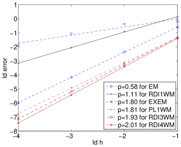
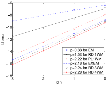
Figure 1: Orders of convergence for SDE (27) and SDE (29).

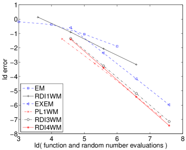
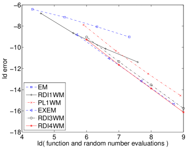
Figure 2: Computational effort per simulation path versus precision for SDE (27) and SDE (29).

Due to the results in Figure 1, we can see that for both test equations the so called optimal SRK scheme RDI1WM attains much better orders of convergence than the well known order one EM scheme. The same holds for the optimal SRK schemes RDI3WM and RDI4WM compared to the order two schemes EXEM and PL1WM. Clearly, the optimal SRK schemes RDI1WM, RDI3WM and RDI4WM need some additional computational effort compared to the schemes EM, EXEM and PL1WM, respectively. Therefore, we take the number of evaluations of the drift function $a$ and of each diffusion function $b^{j}$, $1\leq j\leq m$, as well as the number of random variables that have to be simulated as a measure for the computational effort. Then we can compare the computational effort versus the errors of the analyzed schemes. The results are presented in Figure 2, and again, RDI1WM performs much better than the scheme EM for both test equations. Further, RDI3WM yields similar results like RDI4WM which is for higher precisions slightly better than PL1WM and significantly better than the scheme EXEM for the test equation (27). Considering the multi-dimensional test equation (29), the scheme RDI3WM is again close to RDI4WM which performs for higher precisions slightly better than EXEM. However both optimal SRK schemes RDI3WM and RDI4WM are significantly better than the SRK scheme PL1WM.

6 Conclusion

In the present work, a full classification of the coefficients for a class of explicit SRK methods of order $(1,1)$ for $s=1$ and order $(2,1)$ for $s=2$ stages as well as for the orders $(2,2)$ and $(3,2)$ with $s=3$ stages is calculated. Based on this classification, coefficients for so called optimal SRK schemes are determined by considering additional higher order conditions. Optimal coefficients for SRK methods of order $(2,1)$, $(2,2)$ and $(3,2)$ are calculated and similarly to the deterministic setting [4], better convergence results are expected for these schemes in general. Finally, the SRK schemes based on optimal coefficients are applied to some test equations. Here, it turned out that the proposed optimal SRK schemes attain higher orders of convergence than the well known schemes under consideration and they also perform very well if the computational effort is taken into account.

For future research, it would be interesting to extend the presented classification to diagonal or fully implicit SRK methods. Further, the given classification may be applied in order to determine coefficients for SRK methods with optimal stability properties.

References

- [1] K. Burrage and P. M. Burrage, Order conditions of stochastic Runge–Kutta methods by B-series, SIAM J. Numer. Anal., 38, No. 5, (2000) 1626–1646.
- [2] K. Burrage and P. M. Burrage, High strong order explicit Runge–Kutta methods for stochastic ordinary differential equations, Appl. Numer. Math., 22, No. 1-3, (1996) 81–101.
- [3] J. C. Butcher, The numerical analysis of ordinary differential equations: Runge–Kutta and general linear methods (John Wiley & Sons, Chichester, 1987).
- [4] E. Hairer, S. P. Nørsett and G. Wanner, Solving Ordinary Differential Equations I, Springer-Verlag, Berlin, 1993.
- [5] P. E. Kloeden and E. Platen, Numerical Solution of Stochastic Differential Equations (Applications of Mathematics 23, Springer-Verlag, Berlin, 1999).
- [6] Y. Komori and T. Mitsui and H. Sugiura, Rooted tree analysis of the order conditions of ROW-type scheme for stochastic differential equations, BIT, Vol. 37, No. 1, (1997), 43–66.
- [7] V. Mackevicius and J. Navikas, Second order weak Runge-Kutta type methods for Itô equations, Math. Comput. Simul., Vol. 57, No. 1–2, (2001), 29–34.
- [8] G. N. Milstein, Numerical Integration of Stochastic Differential Equations, Kluwer Academic Publishers, Dordrecht, 1995.
- [9] G. N. Milstein and M. V. Tretyakov, Stochastic Numerics for Mathematical Physics, Scientific Computation, Springer-Verlag, Berlin, 2004.
- [10] A. Rößler, Rooted tree analysis for order conditions of stochastic Runge–Kutta methods for the weak approximation of stochastic differential equations, Stochastic Anal. Appl. Vol. 24, No. 1, (2006), 97–134.
- [11] A. Rößler, Runge–Kutta methods for Itô stochastic differential equations with scalar noise, BIT, Vol. 46, No. 1, (2006), 97–110.
- [12] A. Rößler, Runge–Kutta Methods for the Numerical Solution of Stochastic Differential Equations, Ph.D. thesis, Darmstadt University of Technology. (Shaker Verlag, Aachen, 2003).
- [13] A. Tocino and J. Vigo-Aguiar, Weak second order conditions for stochastic Runge–Kutta methods, SIAM J. Sci. Comput., Vol. 24, No. 2, (2002), 507–523.