Spontaneous symmetry breaking and optimization of functional renormalization group

Abstract

The requirement for the absence of spontaneous symmetry breaking in the $d=1$ dimension has been used to optimize the regulator dependence of functional renormalization group equations in the framework of the sine-Gordon scalar field theory. Results obtained by the optimization of this kind were compared to those of the Litim-Pawlowski and the principle of minimal sensitivity optimization scenarios. The optimal parameters of the compactly supported smooth (CSS) regulator, which recovers all major types of regulators in appropriate limits, have been determined beyond the local potential approximation, and the Litim limit of the CSS was found to be the optimal choice.

I Introduction

Spontaneous symmetry breaking plays an important role in high energy physics or more generally in quantum field theory; as an example one has to mention the mass generation by the Higgs mechanism. However, in the (0+1) dimension as a consequence of the equivalence between quantum field theory and quantum mechanics, a symmetry cannot be broken spontaneously due to tunneling zj ; d1_anharmonic . Thus, for one-dimensional quantum field theoretic models, the spontaneously broken phase should vanish if their phase structures have been determined without using approximations.

Renormalization has relevance in quantum field theory, too, since this procedure is required to obtain measurable physical quantities. It can be performed nonperturbatively by means of the functional renormalization group (RG) method WP ; We1993 ; Mo1994 ; internal which was applied successfully in many cases; let us mention quantum Einstein gravity qeg as a recent example. The functional RG equation for scalar fields We1993

$$k\partial_{k}\Gamma_{k}[\varphi]=\frac{1}{2}{\rm Tr}\left[(k\partial_{k}R_{k})/(\Gamma_{k}^{(2)}[\varphi]+R_{k})\right]$$ (1)

is derived for the blocked effective action $\Gamma_{k}$, which interpolates between the bare $\Gamma_{k\to\Lambda}=S$ and the full quantum effective action $\Gamma_{k\to 0}=\Gamma$ where $k$ is the running momentum scale. The second functional derivative of the blocked action is represented by $\Gamma_{k}^{(2)}$, and the trace Tr stands for the momentum integration. $R_{k}$ is the regulator function where $R_{k}(p\to 0)>0$, $R_{k\to 0}(p)=0$ and $R_{k\to\Lambda}(p)=\infty$. To solve the RG equation (1) one of the commonly used systematic approximations is the truncated derivative (i.e., gradient) expansion where $\Gamma_{k}$ is expanded in powers of the derivative of the field,

$$\Gamma_{k}[\varphi]=\int d^{d}x\left[V_{k}(\varphi)+Z_{k}(\varphi)\frac{1}{2}(\partial_{\mu}\varphi)^{2}+...\right].$$ (2)

Further approximations such as the Taylor or Fourier expansion of $V_{k}(\varphi)$, or $Z_{k}(\varphi)$, are usually also applied. However, the usage of approximations generates two problems: (i) for the $d=1$ dimension the spontaneously broken phase does not vanish in the approximated RG flow, and (ii) physical results obtained by the approximated RG flow become regulator dependent (i.e. renormalization scheme dependent). Therefore, it is of great importance to consider how the approximations used influence the phase structure of one-dimensional models and the comparison of results obtained by various types of regulator functions opt_rg ; litim_o(n) ; opt_func ; Ro2010 ; Mo2005 ; qed2 ; scheme ; scheme_sg ; minimal_sens ; css ; css_pms is also a general issue.

To optimize the scheme dependence, the Litim-Pawlowski optimization method has been worked out opt_rg ; opt_func based on the convergence of the truncated flow that is expanded in powers of the field variable. Its advantage is that in the leading order of the gradient expansion, i.e., in the local potential approximation (LPA), it is possible to find the optimal choice for the parameters of all the regulator functions. Furthermore the Litim’s optimized regulator was constructed, which is expected to provide us with findings closest to ”the best known” results in LPA, e.g. critical exponents of the $O(N)$ scalar theory in $d=3$ dimensions litim_o(n) ; minimal_sens ; scheme ; IR . Its disadvantage is that Litim’s regulator is in conflict with the derivative expansion since it is not a differentiable function.

Another scenario for optimization through the principle of minimal sensitivity (PMS) was also considered minimal_sens . Its advantage is that it can be applied at any order of the derivative expansions for any dimensions; i.e. it is possible to find the optimal choice for the parameters of a particular regulator. Its disadvantage is that one cannot determine the best regulator function among the usual exponential We1993 , power-law Mo1994 and Litim opt_rg regulators through the PMS. However, the combination of the PMS method and the so-called compactly supported smooth (CSS) regulator css provides the tool for optimization where various types of regulators can be directly compared to each other because the CSS recovers the major types of regulators in appropriate limits. This strategy has been successfully applied in LPA css_pms in the framework of the $O(N)$ scalar theory in $d=3$ dimensions and the two-dimensional bosonized quantum electrodynamics (QED₂). In LPA the Litim regulator was found to be the most favorable regulator.

Our goal in this work is to open a new platform to optimize RG equations that represents a suitable optimization scenario beyond LPA. In this new strategy, the requirement of the absence of the broken phase in the case of the nonapproximated RG flow in the $d=1$ dimension is used to optimize the RG scheme dependence of the approximated one. Its advantage is that regulators can be compared to each other at any order of the derivative expansion for $d=1$. It is performed in the framework of the sine-Gordon (SG) model cg_sg which does not require field-dependent wave-function renormalization; thus, the determination of RG equations beyond LPA is simpler than in the case of other models. On the contrary, for the $O(N)$ scalar theory the field-dependent wave function renormalization cannot be avoided. Nevertheless, the new optimization method proposed here can be applied to the $O(N)$ scalar theory in $d=1$, too. After testing the optimization for the power-law regulator Mo1994 , we optimize the CSS regulator css . A similar compactly supported smooth function has been used in nuclear physics sv and the connection to the CSS regulator was shown css .

II Regulator functions

Regulator functions have already been discussed in the literature by introducing its dimensionless form

$$R_{k}(p)=p^{2}r(y),\hskip 14.22636pty=p^{2}/k^{2},$$ (3)

where $r(y)$ is dimensionless. For example, the CSS regulator introduced recently in Ref. css is defined as

$$r_{{\mathrm{css}}}^{{\mathrm{gen}}}(y)=\frac{\exp[cy_{0}^{b}/(f-hy_{0}^{b})]-1}{\exp[cy^{b}/(f-hy^{b})]-1}\theta(f-hy^{b}),$$ (4)

with the Heaviside step function $\theta(y)$. Let us note, that the number of free parameters in (4) can be reduced by setting $f=1$ without loss of generality. The CSS regulator has the property css to recover all major types of regulators: the Litim opt_rg , the power-law Mo1994 and the exponential We1993 ones. By choosing a particular normalization (i.e. fixing $y_{0}$) the CSS regulator reads

$$r_{{\mathrm{css}}}^{{\mathrm{norm}}}(y)= \;\frac{\exp[\ln(2)c]-1}{\exp\left[\frac{\ln(2)cy^{b}}{1-hy^{b}}\right]-1}\theta(1-hy^{b}),$$ (5)

where the limits are

$$\lim_{c\to 0,h\to 1}r_{{\mathrm{css}}}^{{\mathrm{norm}}}= \;\left(\frac{1}{y^{b}}-1\right)\theta(1-y),$$ (6a)

$$\lim_{c\to 0,h\to 0}r_{{\mathrm{css}}}^{{\mathrm{norm}}}= \;\frac{1}{y^{b}},$$ (6b)

$$\lim_{c\to 1,h\to 0}r_{{\mathrm{css}}}^{{\mathrm{norm}}}= \;\frac{1}{\exp[\ln(2)y^{b}]-1}.$$ (6c)

The advantage of this type of normalization is that the form (5) reproduces all the major types of regulators with optimal parameters, i.e. the Litim (6a) with $b=1$, the power-law (6b) with $b=2$, and the exponential (6c) with $b=1.44$. The optimal choices for the parameter $b$ are based on the Litim-Pawlowski optimization scenario.

III SG model for dimensions $1\leq d\leq 2$

To perform the RG study of the SG model sg beyond LPA it is convenient to introduce a dimensionless variable $\tilde{\varphi}=k^{(2-d)/2}\varphi$, and then the effective action reads

$$\Gamma_{k}=\int d^{d}x\left[\frac{1}{2}z_{k}(\partial_{\mu}{\tilde{\varphi}})^{2}+u_{k}\cos(\tilde{\varphi})\right],$$ (7)

where $u_{k}$ is the dimensionful coupling of the periodic self-interaction, $z_{k}$ stands for the field-independent wave-function renormalization that has a dimension of $k^{d-2}$ cg_sg . Although RG transformations generate higher harmonics, we use the ansatz (7) that contains a single Fourier mode since in the case of the SG model it was found to be an appropriate approximation cg_sg . The RG flow equations for the couplings of (7) can be derived from (1)

$$k\partial_{k}u_{k}=\int_{p}\frac{k\partial_{k}R_{k}}{k^{2-d}u_{k}}\left(\frac{P-\sqrt{P^{2}-(k^{2-d}u_{k})^{2}}}{\sqrt{P^{2}-(k^{2-d}u_{k})^{2}}}\right),$$ (8)

$$k\partial_{k}z_{k}=\int_{p}\frac{k\partial_{k}R_{k}}{2}\biggl{[}\frac{-(k^{2-d}u_{k})^{2}P(\partial_{p^{2}}P+\frac{2}{d}p^{2}\partial_{p^{2}}^{2}P)}{[P^{2}-(k^{2-d}u_{k})^{2}]^{5/2}}$$

$$+\frac{(k^{2-d}u_{k})^{2}p^{2}(\partial_{p^{2}}P)^{2}(4P^{2}+(k^{2-d}u_{k})^{2})}{d\,[P^{2}-(k^{2-d}u_{k})^{2}]^{7/2}}\biggr{]},$$ (9)

where $P=z_{k}k^{2-d}p^{2}+R_{k}$ and the momentum integral $\int_{p}=\int dp\,p^{d-1}\Omega_{d}/(2\pi)^{d}$ is usually performed numerically with the $d$-dimensional solid angle $\Omega_{d}$. The RG study of SG type models sg ; qed2 ; qed_qcd does not require field-dependent wave-function renormalization. We use normalized dimensionless parameters $\bar{z}_{k}\equiv(8\pi)\tilde{z}_{k}$ and $\bar{u}_{k}\equiv\tilde{u}_{k}k^{2}/{\bar{k}}$ where $\tilde{z}_{k}=k^{2-d}z_{k}$ and $\tilde{u}_{k}=k^{-d}u_{k}$ are the conventional dimensionless couplings and $\bar{k}=\min_{p^{2}}P$.

In $d=2$ dimensions the SG model undergoes a topological phase transition sg where the critical value that separates the phases of the model, $1/\bar{z}_{\star}=1$, was found to be independent of the choice of the regulator function scheme_sg . For the $d=1$ dimension, based on the approximated RG flow, a saddle point $\bar{u}_{\star}$, $1/\bar{z}_{\star}$ appears in the RG flow cg_sg ; see, for example the results Fig. 1 obtained by the power-law regulator (6b), and thus the SG model has two phases.

Figure 1: Phase diagram of the SG model for $d=1$ dimensions obtained by the numerical solution of Eqs.(8), and (III) using the power-law regulator (6b) with $b=3$. Arrows indicate the direction of the flow. The distance $D$ is defined by (10).

In fractal dimensions, $1<d<2$ the nontrivial saddle point appears in the RG flow, too. However, there is an important difference between the cases of fractal dimensions and of the $d=1$ dimension; namely, the spontaneously broken phase should vanish for $d=1$ which indicates that the saddle point and the nontrivial IR fixed point ($1/\bar{z}_{{\mathrm{IR}}}\equiv 0$, $\bar{u}_{{\mathrm{IR}}}\equiv 1$) should coincide. Thus, the distance between the nontrivial IR fixed point and the saddle point (see Fig. 1),

$$D \equiv \sqrt{(\bar{u}_{{\mathrm{IR}}}-\bar{u}_{\star})^{2}+(1/\bar{z}_{{\mathrm{IR}}}-1/\bar{z}_{\star})^{2}}$$ (10)

$$= \sqrt{(1-\bar{u}_{\star})^{2}+1/\bar{z}_{\star}^{2}}$$

can be used to optimize the scheme dependence of RG equations; i.e., the better the RG scheme the smaller the distance $D$ is. The other attractive IR fixed point ($\bar{u}_{k\to 0}=0$, $1/\bar{z}_{k\to 0}=\infty$) corresponds to the symmetric phase cg_sg ; css .

IV Optimization of the power-law regulator

Let us consider first the optimization of RG equations using the power-law type regulator (6b) in the framework of the SG model. According to the numerical solution of Eqs. (8) and (III), the saddle point appears in the RG flow for dimensions $1\leq d\leq 2$ and its position is plotted in Fig. 2 for various values of the parameter $b$.

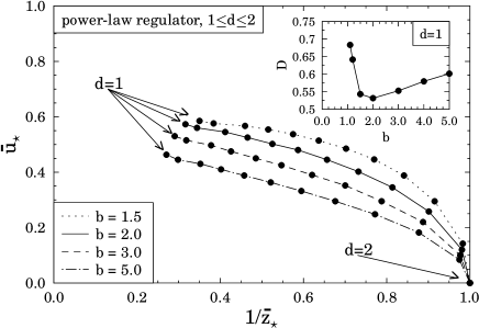
Figure 2: Positions of the saddle point of the SG model for dimensions $1\leq d\leq 2$ obtained by the power-law regulator (6b). The inset shows the dependence of the distance $D$ defined by Eq.(10) on the parameter $b$ for dimension $d=1$.

For $d=2$ dimensions the curves coincide since the fixed point at which the two-dimensional SG model undergoes a topological phase transition is at $\bar{u}_{\star}=0$, $1/\bar{z}_{\star}=1$ scheme independently. For fractal dimensions and also for $d=1$ the position of the saddle point becomes scheme dependent, i.e., it depends on the parameter $b$ of the regulator function (6b). Since the (spontaneously) broken phase should vanish for the $d=1$ dimension, the distance Eq.(10) between the saddle point and the nontrivial IR fixed point ($1/\bar{z}_{{\mathrm{IR}}}\equiv 0$, $\bar{u}_{{\mathrm{IR}}}\equiv 1$) can be used to optimize the RG equation. The inset shows the dependence of the distance $D$ on the parameter $b$ and indicates that $b=2$ is the optimal choice. Thus, it recovers known results obtained by optimization opt_func ; opt_rg based on the optimal convergence of the flow that validates the strategy proposed here.

V Optimization of the CSS regulator

Let us perform the optimization of the normalized CSS regulator (5) in the framework of the one-dimensional SG model using the optimization scenario based on the minimization of the distance $D$ defined by Eq. (10). First, one has to determine the position of the saddle point. This can be done by using the linearized form of RG equations (8), and (III) with dimensionless variables (linearized in terms of $\tilde{u}$) since usually $\tilde{u}_{\star}$ is found to be much smaller than one (after that $\bar{u}_{\star}$, $1/\bar{z}_{\star}$ and the distance $D$ can be calculated). Let us first perform consistency checks. In Fig. 3 we plot the dependence of $D$ on the parameter $b$ of the CSS regulator (5) in various limits. For example, findings determined by the power-law limit (6b) of the CSS regulator (with $c=0.0001$ and $h=0.0001$) is represented by the dashed line which can be compared to the inset of Fig. 2 where results obtained by the exact flow equations (8), and (III) are shown. The two curves are qualitatively the same, and both have a minima at $b\approx 2$ (in case of Fig. 3 it is at $b=2.3$). Let us remind the reader that $b=2$ is the optimal choice according to the Litim-Pawlowski method. Another consistency check is based on the results obtained by the exponential limit (6c) of the CSS regulator (with $c=1$, $h=0.0001$) which is shown by the dotted line in Fig. 3. The minimum (i.e. the optimal choice) is at $b\approx 1.4$ whereas the Litimi-Pawlowski optimization indicates $b=1.44$.

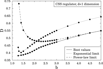
Figure 3: Dependence of $D$ (10) on the parameter $b$ of the CSS regulator (5) represented in various limits. Best values are obtained in terms of the parameters $c$ and $h$, for ”fixed” $b$.

The full line of Fig. 3 shows the minimum (i.e. the best) values of $D$ obtained in terms of the parameters $c$ and $h$, for ”fixed” $b$. For large $b$ it coincides with the power-law limit. It has an inflection point at $b\approx 2.1$ where the power-law and exponential limits cross each other. For small $b$ the best values are obtained for small but nonzero $c$. It also clearly indicates that the most favorable choice is $b\approx 1$. Thus, the Litim limit ($b\approx 1$, $c\approx 0$) of the CSS regulator is found to be the optimal choice beyond LPA (here we use the Litim limit to refer to a small but nonzero value for $c$ and do not take $c\to 0$ exactly). The computation of the best value of $D$ for $b\to 1$ is costly since the derivatives of the CSS regulator for $c\to 0$ have an oscillatory behavior css . Nevertheless for small but finite $c$ the derivatives always exist; hence the Litim limit of the CSS can always be used at any order of the gradient expansion. It does not hold for the Litim regulator itself, which confronts the gradient expansion. Another important observation is that the usage of the PMS method (the global extremum of the CSS) produces exactly the same optimal parameters. Similarly, in LPA css_pms the Litim limit of the CSS with $h=1$ was found to be the most favorable regulator. Beyond LPA the optimal choice for $h$ could depend on the model and also the approximations used. For example, here we found $c=0.1$ and $h\approx 0.3$ as the optimal parameters for $b=1.25$.

VI Summary

A new optimization procedure for the functional RG method has been discussed that is based on the requirement for the absence of spontaneous symmetry breaking in the $d=1$ dimension. It has been applied for the SG model where no field-dependent wave-function renormalization is required; hence the method is suitable for optimization beyond LPA. It is validated by recovering known results on the power-law and exponential regulators. The CSS regulator has been optimized which leads to the best choice among the class of regulator functions. Results were obtained beyond LPA here and the Litim limit of the CSS was found to be the optimal choice. This is supported also by the PMS method that was tested in LPA css_pms for the $O(N)$ model and for QED₂. Therefore, considerations were done for three different models, in three different dimensions at various orders of the derivative expansion with various optimization methods and all these results indicate that the Litim limit of the CSS (small but nonzero $c$) is the most favorable choice.

References

- (1) J. Zinn-Justin, Quantum Field Theory and Critical Phenomena, Clarendon Oxford, (1989).
- (2) A.S. Kapoyannis, N. Tetradis, Phys. Lett. A276, 225 (2000); S. Nagy, K. Sailer, Ann. Phys. (N.Y.) 326, 1839 (2011).
- (3) F. J. Wegner, A. Houghton, Phys. Rev. A 8, 401 (1973); J. Polchinski, Nucl. Phys B 231, 269 (1984).
- (4) C. Wetterich, Nucl. Phys. B352, 529 (1991); ibid, Phys. Lett. B301, 90 (1993); J. Berges, N. Tetradis, C. Wetterich, Phys. Rep. 363, 223 (2002).
- (5) T. R. Morris, Int. J. Mod. Phys. A 09, 2411 (1994).
- (6) J. Alexandre, J. Polonyi, Ann. Phys. (N.Y.) 288, 37 (2001); J. Alexandre, J. Polonyi, K. Sailer, Phys. Lett. B 531, 316 (2002); J. Polonyi, Central Eur. J. Phys.1, 1 (2003).
- (7) M. Reuter, Phys. Rev. D 57, 971 (1998); M. Reuter, F. Saueressig, New J. Phys. 14. 055022 (2012); D. F. Litim, Phys. Rev. Lett. 92, 201301 (2004); M. Reuter, F. Saueressig, Phys. Rev D 65, 065016 (2002); S. Nagy, J. Krizsan, K. sailer, JHEP 07 102 (2012); S. Nagy, arXiv:1211.4151.
- (8) D. F. Litim, Phys. Lett. B 486, 92 (2000); ibid, Phys. Rev. D 64, 105007 (2001); ibid, JHEP 11, 059 (2001).
- (9) D. F. Litim, Nucl.Phys. B 631, 128 (2002).
- (10) T. R. Morris, JHEP 07, 027 (2005).
- (11) O. J. Rosten, Phys. Rept. 511, 177 (2012).
- (12) J. M. Pawlowski, Ann. Phys. (N.Y.) 322, 2831 (2007).
- (13) I. G. Márián, U. D. Jentschura, I. Nándori, arXiv:1311.7377, [J. Phys. G (to be published)].
- (14) I. Nándori, Phys. Rev. D 84, 065024 (2011).
- (15) I. Nándori, S. Nagy, K. Sailer, A. Trombettoni, Phys. Rev. D 80, 025008 (2009); ibid, JHEP 09, 069 (2010).
- (16) L. Canet, B. Delamotte, D. Mouhanna and J. Vidal, Phys. Rev. D 67, 065004 (2003); ibid, Phys.Rev. B 68 064421 (2003); L. Canet, Phys.Rev. B 71 012418 (2005).
- (17) R. D. Ball, P. E. Haagensen, J. I. Latorre and E. Moreno, Phys. Lett. B 347, 80 (1995); D. F. Litim, Phys. Lett. B 393, 103 (1997); K. Aoki, K. Morikawa, W. Souma, J. Sumi and H. Terao, Prog. Theor. Phys. 99, 451 (1998); S.B. Liao, J. Polonyi, M. Strickland, Nucl. Phys. B 567, 493 (2000); J. I. Latorre and T. R. Morris, JHEP 11, 004 (2000); F. Freire and D. F. Litim, Phys. Rev. D 64, 045014 (2001); D. F. Litim, JHEP 07, 005 (2005); C. Bervillier, B. Boisseau, H. Giacomini, Nucl. Phys. B 789, 525 (2008); C. Bervillier, B. Boisseau, H. Giacomini, Nucl. Phys. B 801, 296 (2008); C. S. Fischer, A. Maas, J. M. Pawlowski, Ann. Phys. 324, 2408 (2009); J.M. Caillol, Nucl. Phys. B 855, 854 (2012).
- (18) I. Nándori, JHEP 04, 150 (2013).
- (19) S. Nagy, Nucl. Phys. B 864, 226 (2012); S. Nagy, Phys. Rev. D 86, 085020 (2012); S. Nagy, K. Sailer, Int. J. Mod. Phys. 28, 1350130 (2013).
- (20) I. Nándori, arXiv:1108.4643.
- (21) P. Salamon, T. Vertse, Phys. Rev. C 77, 037302 (2008); P. Salamon, A. T. Kruppa, T. Vertse, Phys. Rev. C 81, 064322 (2010).
- (22) S. R. Coleman Phys. Rev. D 11, 2088 (1975); I. Nándori, J. Polonyi, K. Sailer, Phys. Rev. D 63, 045022 (2001); S. Nagy, K. Sailer, J. Polonyi, J. Phys. A 39, 8105 (2006); S. Nagy, I. Nándori, J. Polonyi, K. Sailer, Phys. Lett. B 647, 152 (2007); V. Pangon, S. Nagy, J. Polonyi, K. Sailer, Phys. Lett. B 694, 89 (2010); I. Nándori, U. D. Jentschura, K. Sailer, G. Soff, Phys. Rev. D 69, 025004 (2004); S. Nagy, I. Nándori, J. Polonyi, K. Sailer, Phys. Rev. Lett. 102 241603 (2009); J. Alexandre, D. Tanner, Phys. Rev. D 82, 125035 (2010); V. Pangon, Int. J. Mod. Phys. A 27, 1250014 (2012).
- (23) S. Nagy, J. Polonyi, K. Sailer, Phys. Rev. D 70, 105023 (2004); I. Nándori, J. Phys. A: Math. Gen. 39, 8119 (2006); I. Nándori, Phys. Lett. B 662, 302 (2008); S. Nagy, Phys. Rev. D 79, 045004 (2009); J. Kovács, S. Nagy, I. Nándori, K. Sailer, JHEP 01, 126 (2011).