A distributed adaptive steplength stochastic approximation method
for monotone stochastic Nash Games

Abstract

We consider a distributed stochastic approximation (SA) scheme for computing an equilibrium of a stochastic Nash game. Standard SA schemes employ diminishing steplength sequences that are square summable but not summable. Such requirements provide a little or no guidance for how to leverage Lipschitzian and monotonicity properties of the problem and naive choices (such as $\gamma_{k}=1/k$) generally do not preform uniformly well on a breadth of problems. While a centralized adaptive stepsize SA scheme is proposed in [1] for the optimization framework, such a scheme provides no freedom for the agents in choosing their own stepsizes. Thus, a direct application of centralized stepsize schemes is impractical in solving Nash games. Furthermore, extensions to game-theoretic regimes where players may independently choose steplength sequences are limited to recent work by Koshal et al. [2]. Motivated by these shortcomings, we present a distributed algorithm in which each player updates his steplength based on the previous steplength and some problem parameters. The steplength rules are derived from minimizing an upper bound of the errors associated with players’ decisions. It is shown that these rules generate sequences that converge almost surely to an equilibrium of the stochastic Nash game. Importantly, variants of this rule are suggested where players independently select steplength sequences while abiding by an overall coordination requirement. Preliminary numerical results are seen to be promising.

I Introduction

We consider a class of stochastic Nash games in which every player solves a stochastic convex program parametrized by adversarial strategies. Consider an $N$-person stochastic Nash game in which the $i$th player solves the parametrized convex problem

$$\min_{x\in X_{i}}\mathsf{E}\!\left[f_{i}(x_{i},x_{-i},\xi_{i})\right],$$ (1)

where $x_{-i}$ denotes the collection $\{x_{j},j\neq i\}$ of decisions of all players other than player $i$. For each $i$, the vector $\xi_{i}:\Omega_{i}\rightarrow\mathbb{R}^{n_{i}}$ is a random vector with a probability distribution on some set, while the function $\mathsf{E}\!\left[f_{i}(x_{i},x_{-i},\xi_{i})\right]$ is strongly convex in $x_{i}$ for all $x_{-i}\in\prod_{j\neq i}X_{j}$. For every $i$, the set $X_{i}\subseteq\mathbb{R}^{n_{i}}$ is closed and convex. We focus on the resulting stochastic variational inequality (VI) and consider the development of distributed stochastic approximation schemes that rely on adaptive steplength sequences. Stochastic approximation techniques have a long tradition. First proposed by Robbins and Monro [3] for differentiable functions and Ermoliev [4, 5, 6], significant effort has been applied towards theoretical and algorithmic examination of such schemes (cf. [7, 8]). Yet, there has been markedly little on the application of such techniques to solution of stochastic variational inequalities. Exceptions include the work by Jiang and Xu [9], and more recently by Koshal et al. [2]. The latter, in particular, develops a single timescale stochastic approximation scheme for precisely the class of problems being studied here viz. monotone stochastic Nash games.

Standard stochastic approximation schemes provide little guidance regarding the choice of a steplength sequence, apart from requiring that the sequence, denoted by $\{\gamma_{k}\}$, satisfies $\sum_{k=1}^{\infty}\gamma_{k}=\infty\mbox{ and }\sum_{k=1}^{\infty}\gamma_{k}^{2}<\infty.$ This paper is motivated by the need to develop adaptive steplength sequences that can be independently chosen by players under a limited coordination, while guaranteeing the overall convergence of the scheme. Adaptive stepsizes have been effectively used in gradient and subgradient algorithms. Vrahatis et al. [10] presented a class of gradient algorithms with adaptive stepsizes for unconstrained minimization. Spall [11] developed a general adaptive SA algorithm based on using a simultaneous perturbation approach for estimating the Hessian matrix. Cicek et al. [12] considered the Kiefer-Wolfowitz (KW) SA algorithm and derived general upper bounds on its mean-squared error, together with an adaptive version of the KW algorithm. Ram et al. [13] considered distributed stochastic subgradient algorithms for convex optimization problems and studied the effects of stochastic errors on the convergence of the proposed algorithm. Lizarraga et al. [14] considered a family of two person Mutil-Plant game and developed Stackelberg-Nash equilibrium conditions based on the Robust Maximum Principle. More recently, Yousefian et al. [1, 15] developed centralized adaptive stepsize SA schemes for solving stochastic optimization problems and variational inequalities. The main contribution of the current paper lies in developing a class of distributed adaptive stepsize rules for SA scheme in which each agent chooses its own stepsizes without any specific information about other agents stepsize policy. This degree of freedom in choosing the stepsizes has not been addressed in the centralized schemes.

Before proceeding, we briefly motivate the question of distributed computation of Nash equilibria from two different standpoints: (i) First, the Nash game can be viewed as a competitive analog of a stochastic multi-user convex optimization problem of the form $\min_{{\color[rgb]{0,0,0}x\in X}}\sum_{i=1}^{N}\mathsf{E}\!\left[f_{i}(x_{i},x_{-i},\xi_{i})\right].$ Furthermore, under the assumption that equilibria of the associated stochastic Nash game are efficient, our scheme provides a distributed framework for computing solutions to this problem. In such a setting, we may prescribe that players employ stochastic approximation schemes since the Nash game represents an engineered construct employed for computing solutions; (ii) A second perspective is one drawn from a bounded rationality approach towards distributed computation of Nash equilibria. A fully rational avenue for computing equilibria suggests that each player employs a best response mapping in updating strategies, based on what the competing players are doing. Yet, when faced by computational or time constraints, players may instead take a gradient step. We work in precisely this regime but allow for flexibility in terms of the steplengths chosen by the players.

In this paper, we consider the solution of a stochastic Nash game whose equilibria are completely captured by a stochastic variational inequality with a strongly monotone mapping. Motivated by the need for efficient distributed simulation methods for computing solutions to such problems, we present a distributed scheme in which each player employs an adaptive rule for prescribing steplengths. Importantly, these rules can be implemented with relatively little coordination by any given player and collectively lead to iterates that are shown to converge to the unique equilibrium in an almost-sure sense.

This paper is organized as follows. In Section II, we introduce the formulation of a stochastic Nash games in which every player solves a stochastic convex problem. In Section III, we show the almost-sure convergence of the SA algorithm under specified assumptions. In Section IV, motivated by minimizing a suitably defined error bound, we develop an adaptive steplength stochastic approximation framework in which every player adaptively updates his steplength. It is shown that the choice of adaptive steplength rules can be obtained independently by each player under a limited coordination. Finally, in Section V, we provide some numerical results from a stochastic flow management game drawn from a communication network setting.

Notation: Throughout this paper, a vector $x$ is assumed to be a column vector. We write $x^{T}$ to denote the transpose of a vector $x$. $\|x\|$ denotes the Euclidean vector norm, i.e., $\|x\|=\sqrt{x^{T}x}$. We use $\Pi_{X}(x)$ to denote the Euclidean projection of a vector $x$ on a set $X$, i.e., $\|x-\Pi_{X}(x)\|=\min_{y\in X}\|x-y\|$. Vector $g$ is a subgradient of a convex function $f$ with domain dom$f$ at $\bar{x}\in\hbox{dom}f$ when $f(\bar{x})+g^{T}(x-\bar{x})\leq f(x)$ for all $x\in\hbox{dom}f.$ The set of all subgradients of $f$ at $\bar{x}$ is denoted by $\partial f(\bar{x})$. We write a.s. as the abbreviation for “almost surely”, and use $\mathsf{E}\!\left[z\right]$ to denote the expectation of a random variable $z$.

II Problem formulation

In this section, we present (sufficient) conditions associated with equilibrium points of the stochastic Nash game defined by (1). The equilibrium conditions of this game can be characterized by a stochastic variational inequality problem denoted by VI$(X,F)$, where

$$F(x)\triangleq\left(\begin{array}[]{ccc}\nabla_{x_{1}}\mathsf{E}\!\left[f_{1}(x,\xi_{1})\right]\\ \vdots\\ \nabla_{x_{N}}\mathsf{E}\!\left[f_{N}(x,\xi_{N})\right]\end{array}\right),\quad X=\prod_{i=1}^{N}X_{i},$$ (5)

with $x\triangleq(x_{1},\ldots,x_{N})^{T}$ and $x_{i}\in X_{i}{\subseteq\mathbb{R}^{n_{i}}}$ for $i=1,\ldots,N$. Given a set $X\subseteq\mathbb{R}^{n}$ and a single-valued mapping $F:X\to\mathbb{R}^{n}$, then a vector $x^{*}\in X$ solves a variational inequality VI$(X,F)$, if

$$(x-x^{*})^{T}F(x^{*})\geq 0\hbox{ for all }x\in X.$$ (6)

Let $n=\sum_{i=1}^{N}n_{i}$, and note that when the sets $X_{i}$ are convex and closed for all $i$, the set $X\in\mathbb{R}^{n}$ is closed and convex.

In the context of solving the stochastic variational inequality VI$(X,F)$ in (5)-(6), suppose each player employs a stochastic approximation scheme for given by

$$\begin{aligned} x_{{k+1},i}&=\Pi_{X_{i}}\left(x_{k,i}-\gamma_{k,i}(F_{i}(x_{k})+w_{k,i})\right),\cr w_{k,i}&\triangleq\hat{F}_{i}(x_{k},\xi_{k})-F_{i}(x_{k}),\end{aligned}$$ (7)

for all $k\geq 0$ and $i=1,\dots,N$, where $\gamma_{k,i}>0$ is the stepsize of the $i$th player at iteration $k$, $x_{k}=(x_{k,1}\ x_{k,2}\ \ldots\ x_{k,N})^{T}$, $\xi_{k}=(\xi_{k,1}\ \xi_{k,2}\ \ldots\ \xi_{k,N})^{T}$, $F_{i}=\mathsf{E}\!\left[\nabla_{x_{i}}f_{i}(x,\xi_{i})\right]$, and

$$\hat{F}(x,\xi)\triangleq\left(\begin{array}[]{ccc}\nabla_{x_{1}}f_{1}(x,\xi_{1})\\ \vdots\\ \nabla_{x_{N}}{f_{N}(x,\xi_{N})}\end{array}\right),\quad\xi\triangleq\left(\begin{array}[]{ccc}\xi_{1}\\ \vdots\\ \xi_{N}\end{array}\right).$$

Note that in terms of the definition of $w_{k,i}$, $F_{i}$, and $\hat{F}_{i}$, $\mathsf{E}\!\left[w_{k,i}\mid\mathcal{F}_{k}\right]=0.$ In addition, $x_{0}\in X$ is a random initial vector independent of the random variable $\xi$ and such that $\mathsf{E}\!\left[\|x_{0}\|^{2}\right]<\infty$. Note that each player uses its individual stepsize to update its decision.

III A Distributed SA scheme

In this section, we present conditions under which algorithm (7) converges almost surely to the solution of game (1) under suitable assumptions on the mapping. Also, we develop a distributed variant of a standard stochastic approximation scheme and provide conditions on the steplength sequences that lead to almost-sure convergence of the iterates to the unique solution. Our assumptions include requirements on the set $X$ and the mapping $F$.

Assumption 1

Assume the following:

1. The sets $X_{i}\subseteq\mathbb{R}^{n_{i}}$ are closed and convex.

2. $F(x)$ is strongly monotone with constant $\eta>0$ and Lipschitz continuous with constant $L$ over the set $X$.

Remark: The strong monotonicity is assumed to hold throughout the paper. Although the convergence results may still hold with a weaker assumption, such as strict monotonicity, but the stepsize policy in this paper leverages the strong monotonicity parameter which prescribes a more parametrized stepsize rule. This is the main reason that we assumed the stronger version of monotonicity. In Section V, we present an example where such an assumption is satisfied.

Another set of assumptions is for the stepsizes employed by each player in algorithm (7).

Assumption 2

Assume that:

1. The stepsize sequences are such that $\gamma_{k,i}>0$ for all $k$ and $i$, with $\sum_{k=0}^{\infty}\gamma_{k,i}=\infty$ and $\sum_{k=0}^{\infty}\gamma_{k,i}^{2}<\infty$.

2. There exists a scalar $\beta$ such that $0\leq\beta<\frac{\eta}{L}$ and $\frac{\Gamma_{k}-\delta_{k}}{\delta_{k}}\leq\beta$ for all $k\geq 0$, where $\delta_{k}$ and $\Gamma_{k}$ are (fixed) positive sequences satisfying $\delta_{k}\leq\min_{i=1,\ldots,N}{\gamma_{k,i}}$ and $\Gamma_{k}\geq\max_{i=1,\ldots,N}{\gamma_{k,i}}$ for all $k\geq 0$.

We let $\mathcal{F}_{k}$ denote the history of the method up to time $k$, i.e., $\mathcal{F}_{k}=\{x_{0},\xi_{0},\xi_{1},\ldots,\xi_{k-1}\}$ for $k\geq 1$ and $\mathcal{F}_{0}=\{x_{0}\}$. Consider the following assumption on the stochastic errors, $w_{k}$, of the algorithm.

Assumption 3

The errors $w_{k}$ are such that for some constant $\nu>0$,

$$\mathsf{E}\!\left[\|w_{k}\|^{2}\mid\mathcal{F}_{k}\right]\leq\nu^{2}\qquad\hbox{{a.s.} for all $k\geq 0$}.$$

We use the Robbins-Siegmund lemma in establishing the convergence of method (7), which can be found in [16] (cf. Lemma 10, page 49).

Lemma 1

Let $\{v_{k}\}$ be a sequence of nonnegative random variables, where $\mathsf{E}\!\left[v_{0}\right]<\infty$, and let $\{\alpha_{k}\}$ and $\{\mu_{k}\}$ be deterministic scalar sequences such that:

$$\mathsf{E}\!\left[v_{k+1}|v_{0},\ldots,v_{k}\right]\leq(1-\alpha_{k})v_{k}+\mu_{k}\qquad a.s.\ \hbox{for all }k\geq 0,$$

$$0\leq\alpha_{k}\leq 1,\quad\ \mu_{k}\geq 0,$$

$$\quad\ \sum_{k=0}^{\infty}\alpha_{k}=\infty,\quad\ \sum_{k=0}^{\infty}\mu_{k}<\infty,\quad\ \lim_{k\to\infty}\,\frac{\mu_{k}}{\alpha_{k}}=0.$$

Then, $v_{k}\rightarrow 0$ almost surely.

The following lemma provides an error bound for algorithm (7) under Assumption 1.

Lemma 2

Consider algorithm (7). Let Assumption 1 hold. Then, the following relation holds a.s. for all $k\geq 0$:

$$\mathsf{E}\!\left[\|x_{k+1}-x^{*}\|^{2}\mid\mathcal{F}_{k}\right]\leq\Gamma_{k}^{2}\mathsf{E}\!\left[\|w_{k}\|^{2}\mid\mathcal{F}_{k}\right]$$ (8)

$$+(1-2(\eta+L)\delta_{k}+2L\Gamma_{k}+L^{2}\Gamma_{k}^{2})\|x_{k}-x^{*}\|^{2}.$$ (9)

Proof:

By Assumption 1a, the set $X$ is closed and convex. Since $F$ is strongly monotone, the existence and uniqueness of the solution to VI$(X,F)$ is guaranteed by Theorem 2.3.3 of [17]. Let $x^{*}$ denote the solution of VI$(X,F)$. From properties of projection operator, we know that a vector $x^{*}$ solves VI$(X,F)$ problem if and only if $x^{*}$ satisfies

$$x^{*}=\Pi_{X}(x^{*}-\gamma F(x^{*}))\qquad\hbox{for any }\gamma>0.$$

From algorithm (7) and the non-expansiveness property of the projection operator, we have for all $k\geq 0$ and $i$,

$$\|x_{k+1,i}-x_{i}^{*}\|^{2}=\|\Pi_{X_{i}}(x_{k,i}-\gamma_{k,i}(F_{i}(x_{k})+w_{k,i}))$$

$$-\Pi_{X_{i}}(x_{i}^{*}-\gamma_{k,i}F_{i}(x^{*}))\|^{2}$$

$$\leq\|x_{k,i}-x_{i}^{*}-\gamma_{k,i}(F_{i}(x_{k})+w_{k,i}-F_{i}(x^{*}))\|^{2}.$$

Taking the expectation conditioned on the past, and using $\mathsf{E}\!\left[w_{k,i}\mid\mathcal{F}_{k}\right]=0$, we have

$$\mathsf{E}\!\left[\|x_{k+1,i}-x_{i}^{*}\|^{2}\mid\mathcal{F}_{k}\right]\leq\|x_{k,i}-x_{i}^{*}\|^{2}$$

$$+\gamma_{k,i}^{2}\|F_{i}(x_{k})-F_{i}(x^{*})\|^{2}+\gamma_{k,i}^{2}\mathsf{E}\!\left[\|w_{k,i}\|^{2}\mid\mathcal{F}_{k}\right]$$

$$-2\gamma_{k,i}(x_{k,i}-x_{i}^{*})^{T}(F_{i}(x_{k})-F_{i}(x^{*})).$$

Now, by summing the preceding relations over $i$, we have

$$\mathsf{E}\!\left[\|x_{k+1}-x^{*}\|^{2}\mid\mathcal{F}_{k}\right]\leq\|x_{k}-x^{*}\|^{2}$$ (10)

$$+\underbrace{\sum_{i=1}^{N}\gamma_{k,i}^{2}\|F_{i}(x_{k})-F_{i}(x^{*})\|^{2}}_{\bf Term\,1}+\sum_{i=1}^{N}\gamma_{k,i}^{2}\mathsf{E}\!\left[\|w_{k,i}\|^{2}\mid\mathcal{F}_{k}\right]$$ (11)

$$\underbrace{-2\sum_{i=1}^{N}\gamma_{k,i}(x_{k,i}-x_{i}^{*})^{T}(F_{i}(x_{k})-F_{i}(x^{*}))}_{\bf Term\,2}.$$ (12)

Next, we estimate Term $1$ and Term $2$ in (10). By using the definition of $\Gamma_{k}$ and by leveraging the Lipschitzian property of mapping $F$, we obtain

$$\hbox{Term}\,1\leq\Gamma_{k}^{2}\|F(x_{k})-F(x^{*})\|^{2}\leq\Gamma_{k}^{2}L^{2}\|x_{k}-x^{*}\|^{2}.$$ (13)

Adding and subtracting $-2\sum_{i=1}^{N}\delta_{k}(x_{k,i}-x_{i}^{*})^{T}(F_{i}(x_{k})-F_{i}(x^{*}))$ from Term $2$, we further obtain

$$\begin{split}\hbox{Term}\,2\leq&-2\delta_{k}(x_{k}-x^{*})^{T}(F(x_{k})-F(x^{*}))\cr&-2\sum_{i=1}^{N}(\gamma_{k,i}-\delta_{k})(x_{k,i}-x_{i}^{*})^{T}{(F_{i}(x_{k})-F_{i}(x^{*}))}.\end{split}$$

By the Cauchy-Schwartz inequality, we obtain

$$\begin{split}\hbox{Term}\,2\leq&-2\delta_{k}(x_{k}-x^{*})^{T}(F(x_{k})-F(x^{*}))\cr&+2(\gamma_{k,i}-\delta_{k})\sum_{i=1}^{N}\|x_{k,i}-x_{i}^{*}\|\|{F_{i}(x_{k})-F_{i}(x^{*})}\|\cr\leq&-2\delta_{k}(x_{k}-x^{*})^{T}(F(x_{k})-F(x^{*}))\cr&+2(\Gamma_{k}-\delta_{k})\|x_{k}-x^{*}\|\|F(x_{k})-F(x^{*})\|,\end{split}$$

where in the last relation, we use Hölder’s inequality. Invoking the strong monotonicity of the mapping for bounding the first term and by utilizing the Lipschitzian property of the second term of the preceding relation, we have

$$\begin{split}\hbox{Term}\,2\leq-2\eta\delta_{k}\|x_{k}-x^{*}\|^{2}+2(\Gamma_{k}-\delta_{k})L\|x_{k}-x^{*}\|^{2}.\end{split}$$

The desired inequality is obtained by combining relations (10) and (13) with the preceding inequality . ∎

We next prove that algorithm (7) generates a sequence of iterates that converges a.s. to the unique solution of VI$(X,F)$, as seen in the following proposition. Our proof of this result makes use of Lemma 2.

Proposition 1 (Almost-sure convergence)

Consider the algorithm 7. Let Assumption 1, 2 and 3 hold. Then,

1. The following relation holds a.s. for all $k\geq 0$:

   $$\mathsf{E}\!\left[\|x_{k+1}-x^{*}\|^{2}\right]\leq(1+\beta)^{2}\delta_{k}^{2}\nu^{2}$$

   $$+(1-2(\eta-\beta L)\delta_{k}+(1+\beta)^{2}L^{2}\delta_{k}^{2})\mathsf{E}\!\left[\|x_{k}-x^{*}\|^{2}\right].$$

2. The sequence $\{x_{k}\}$ generated by algorithm (7), converges a.s. to the unique solution of VI$(X,F)$.

Proof:

(a)  Assumption 2b implies that $\Gamma_{k}\leq(1+\beta)\delta_{k}$. Combining this with inequality (8), we obtain

$$\mathsf{E}\!\left[\|x_{k+1}-x^{*}\|^{2}\mid\mathcal{F}_{k}\right]$$

$$\leq(1-2(\eta-\beta L)\delta_{k}+(1+\beta)^{2}L^{2}\delta_{k}^{2})\|x_{k}-x^{*}\|^{2}$$

$$+(1+\beta)^{2}\delta_{k}^{2}\mathsf{E}\!\left[\|w_{k}\|^{2}\mid\mathcal{F}_{k}\right],\qquad\hbox{for all }k\geq 0.$$

Taking expectations in the preceding inequality and using Assumption 3, we obtain the desired relation.

(b)  We show that the conditions of Lemma 1 are satisfied in order to claim almost sure convergence of $x_{k}$ to $x^{*}$. Let us define $v_{k}\triangleq\|x_{k+1}-x^{*}\|^{2}$, $\alpha_{k}\triangleq 2(\eta-\beta L)\delta_{k}-L^{2}\delta_{k}^{2}(1+\beta)^{2}$, and $\mu_{k}\triangleq(1+\beta)^{2}\delta_{k}^{2}\mathsf{E}\!\left[\|w_{k}\|^{2}\mid\mathcal{F}_{k}\right]$. Since $\gamma_{k,i}$ tends to zero for any $i=1,\ldots,N$, we may conclude that $\delta_{k}$ goes to zero as $k$ grows. Recall that $\alpha_{k}$ is given by

$$\alpha_{k}=2(\eta-\beta L)\delta_{k}\left(1-\frac{(1+\beta)^{2}L^{2}\delta_{k}}{2(\eta-\beta L)}\right).$$

Due to $\delta_{k}\to 0$, for all $k$ large enough, say $k>k_{1}$, we have

$$1-\frac{(1+\beta)^{2}L^{2}\delta_{k}}{2(\eta-\beta L)}>0.$$

Since $\beta<\frac{\eta}{L}$ (Assumption 2b), it follows $\eta-\beta L>0$. Thus, we have $\alpha_{k}\geq 0$. Also, for $k$ large enough, say $k>k_{2}$, we have $\alpha_{k}\leq 1$. Therefore, when $k>\max\{k_{1},k_{2}\}$ we have $0\leq\alpha_{k}\leq 1$. Obviously, $v_{k},\mu_{k}\geq 0$. From Assumption 2a and Assumption 3 it follows $\sum_{k}\mu_{k}<\infty$. We also have

$${\lim_{k\rightarrow\infty}}\frac{\mu_{k}}{\alpha_{k}} ={\lim_{k\rightarrow\infty}}\frac{(1+\beta)^{2}\delta_{k}^{2}\mathsf{E}\!\left[\|w_{k}\|^{2}\mid\mathcal{F}_{k}\right]}{2(\eta-\beta L)\delta_{k}\left(1-\frac{(1+\beta)^{2}L^{2}\delta_{k}}{2(\eta-\beta L)}\right)}$$

$$={\lim_{k\rightarrow\infty}}\frac{(1+\beta)^{2}\delta_{k}\mathsf{E}\!\left[\|w_{k}\|^{2}\mid\mathcal{F}_{k}\right]}{2(\eta-\beta L)}.$$

Since the term $\mathsf{E}\!\left[\|w_{k}\|^{2}\mid\mathcal{F}_{k}\right]$ is bounded by $\nu^{2}$ (Assumption 3) and $\delta_{k}\to 0$, we see that $\lim_{k\rightarrow\infty}\frac{\mu_{k}}{\alpha_{k}}=0$. Hence, the conditions of Lemma 1 are satisfied, which implies that $x_{k}$ converges to the unique solution, $x^{*}$, almost surely. ∎

Consider now a special form of algorithm (7) corresponding to the case when all players employ the same stepsize, i.e., $\gamma_{k,i}=\gamma_{k}$ for all $k$. Then, the algorithm (7) reduces to the following:

$$\begin{aligned} x_{k+1}&=\Pi_{X}\left(x_{k}-\gamma_{k}(F(x_{k})+w_{k})\right),\cr w_{k}&\triangleq\hat{F}(x_{k},\xi_{k})-F(x_{k}),\end{aligned}$$ (14)

for all $k\geq 0$. Observe that when $\gamma_{k,i}=\gamma_{k}$ for all $k$, Assumption 2a is satisfied when $\sum_{k=0}^{\infty}\gamma_{k}=\infty$ and $\sum_{k=0}^{\infty}\gamma_{k}^{2}<\infty$. Assumption 2b is automatically satisfied with $\Gamma_{k}=\delta_{k}=\gamma_{k}$ and $\beta=0$. Hence, as a direct consequence of Proposition 1, we have the following corollary.

Corollary 1 (Identical stepsizes)

Consider algorithm (14). Let Assumption 1 and 3 hold. Also, let $\sum_{k=0}^{\infty}\gamma_{k}=\infty$ and $\sum_{k=0}^{\infty}\gamma_{k}^{2}<\infty$. Then,

1. The following relation holds almost surely:

   $$\mathsf{E}\!\left[\|x_{k+1}-x^{*}\|^{2}\right] \leq(1-2\eta\gamma_{k}+L^{2}\gamma_{k}^{2})\mathsf{E}\!\left[\|x_{k}-x^{*}\|^{2}\right]$$

   $$+\gamma_{k}^{2}\nu^{2}.$$

2. The sequence $\{x_{k}\}$ generated by algorithm (14), converges a.s. to the unique solution of VI$(X,F)$.

IV A distributed adaptive steplength SA scheme

Stochastic approximation algorithms require stepsize sequences to be square summable but not summable. These algorithms provide little advice regarding the choice of such sequences. One of the most common choices has been the harmonic steplength rule which takes the form of $\gamma_{k}=\frac{\theta}{k}$ where $\theta>0$ is a constant. Although, this choice guarantees almost-sure convergence, it does not leverage problem parameters. Numerically, it has been observed that such choices can perform quite poorly in practice. Motivated by this shortcoming, we present a distributed adaptive steplength scheme for algorithm (7) which guarantees almost-sure convergence of $x_{k}$ to the unique solution of VI$(X,F)$. It is derived from the minimizer of a suitably defined error bound and leads to a recursive relation; more specifically, at each step, the new stepsize is calculated using the stepsize from the preceding iteration and problem parameters. To begin our analysis, we consider the result of Proposition 1a for all $k\geq 0$:

$$\mathsf{E}\!\left[\|x_{k+1}-x^{*}\|^{2}\right]\leq(1+\beta)^{2}\delta_{k}^{2}\nu^{2}$$ (15)

$$+(1-2(\eta-\beta L)\delta_{k}+(1+\beta)^{2}L^{2}\delta_{k}^{2})\mathsf{E}\!\left[\|x_{k}-x^{*}\|^{2}\right].\quad$$ (16)

When the stepsizes are further restricted so that

$$0<\delta_{k}\leq\frac{\eta-\beta L}{(1+\beta)^{2}L^{2}},$$

we have

$$1-2(\eta-\beta L)\delta_{k}+L^{2}(1+\beta)^{2}\delta_{k}^{2}\leq 1-(\eta-\beta L)\delta_{k}.$$

Thus, for $0<\delta_{k}\leq\frac{\eta-\beta L}{(1+\beta)^{2}L^{2}}$, from inequality (15) we obtain

$$\mathsf{E}\!\left[\|x_{k+1}-x^{*}\|^{2}\right] \leq(1-(\eta-\beta L)\delta_{k})\mathsf{E}\!\left[\|x_{k}-x^{*}\|^{2}\right]$$ (17)

$$+(1+\beta)^{2}\delta_{k}^{2}\nu^{2}\qquad\hbox{for all }k\geq 0.\quad$$ (18)

Let us view the quantity $\mathsf{E}\!\left[\|x_{k+1}-x^{*}\|^{2}\right]$ as an error $e_{k+1}$ of the method arising from the use of the stepsize values $\delta_{0},\delta_{1},\ldots,\delta_{k}$. Relation (17) gives us an estimate of the error of algorithm (7). We use this estimate to develop an adaptive stepsize procedure. Consider the worst case which is the case when  (17) holds with equality. In this worst case, the error satisfies the following recursive relation:

$$e_{k+1}=(1-(\eta-\beta L)\delta_{k})e_{k}+(1+\beta^{2})\delta_{k}^{2}\nu^{2}.$$

Let us assume that we want to run the algorithm (7) for a fixed number of iterations, say $K$. The preceding relation shows that $e_{K}$ depends on the stepsize values up to the $K$th iteration. This motivates us to see the stepsize parameters as decision variables that can minimize a suitably defined error bound of the algorithm. Thus, the variables are $\delta_{0},\delta_{1},\ldots,\delta_{K-1}$ and the objective function is the error function $e_{K}(\delta_{0},\delta_{1},\ldots,\delta_{K-1})$. We proceed to derive a stepsize rule by minimizing the error $e_{K+1}$; Importantly, $\delta_{K+1}$ can be shown to be a function of only the most recent stepsize $\delta_{K}$. We define the real-valued error function $e_{k}(\delta_{0},\delta_{1},\ldots,\delta_{k-1})$ by the upper bound in (17):

$$e_{k+1}(\delta_{0},\ldots,\delta_{k})\triangleq (1-(\eta-\beta L)\delta_{k})e_{k}(\delta_{0},\ldots,\delta_{k-1})$$ (19)

$$+(1+\beta^{2})\delta_{k}^{2}\nu^{2}\qquad\hbox{for all }k\geq 0,$$ (20)

where $e_{0}$ is a positive scalar, $\eta$ is the strong monotonicity parameter and $\nu^{2}$ is the upper bound for the second moments of the error norms $\|w_{k}\|$.

Now, let us consider the stepsize sequence $\{\delta^{*}_{k}\}$ given by

$$\delta_{0}^{*}=\frac{\eta-\beta L}{2(1+\beta)^{2}\nu^{2}}\,e_{0}$$ (21)

$$\delta_{k}^{*}=\delta_{k-1}^{*}\left(1-\frac{\eta-\beta L}{2}\delta_{k-1}^{*}\right)\quad\hbox{for all }k\geq 1.$$ (22)

In what follows, we often abbreviate $e_{k}(\delta_{0},\ldots,\delta_{k-1})$ by $e_{k}$ whenever this is unambiguous. The next proposition shows that the lower bound sequence of $\gamma_{k,i}$ given by (21)–(22) minimizes the errors $e_{k}$ over $(0,\frac{\eta-\beta L}{(1+\beta)^{2}L^{2}}]^{k}$.

Proposition 2

Let $e_{k}(\delta_{0},\ldots,\delta_{k-1})$ be defined as in (19), where $e_{0}>0$ is such that $\,e_{0}<\frac{2\nu^{2}}{L^{2}}$, and $L$ is the Lipschitz constant of mapping $F$. Let the sequence $\{\delta^{*}_{k}\}$ be given by (21)–(22). Then, the following hold:

• $e_{k}(\delta_{0}^{*},\ldots,\delta_{k}^{*})=\frac{2(1+\beta)^{2}\nu^{2}}{\eta-\beta L}\,\delta_{k}^{*}$ for all $k\geq 0$.

• For any $k\geq 1$, the vector $(\delta_{0}^{*},\delta_{1}^{*},\ldots,\delta_{k-1}^{*})$ is the minimizer of the function $e_{k}(\delta_{0},\ldots,\delta_{k-1})$ over the set

  $$\mathbb{G}_{k}\triangleq\left\{\alpha\in\mathbb{R}^{k}:0<\alpha_{j}\leq\frac{\eta-\beta L}{(1+\beta)^{2}L^{2}},j=1,\ldots,k\right\},$$

  i.e., for any $k\geq 1$ and $(\delta_{0},\ldots,\delta_{k-1})\in\mathbb{G}_{k}$:

  $$e_{k}(\delta_{0},\ldots,\delta_{k-1})-e_{k}(\delta_{0}^{*},\ldots,\delta_{k-1}^{*})$$

  $$\geq(1+\beta)^{2}\nu^{2}(\delta_{k-1}-\delta_{k-1}^{*})^{2}.$$

Proof:

(a)  To show the result, we use induction on $k$. Trivially, it holds for $k=0$ from (21). Now, suppose that we have $e_{k}(\delta_{0}^{*},\ldots,\delta_{k-1}^{*})=\frac{2(1+\beta)^{2}\nu^{2}}{\eta-\beta L}\,\delta_{k}^{*}$ for some $k$, and consider the case for $k+1$. From the definition of the error $e_{k}$ in (19) and the inductive hypothesis, we have

$$e_{k+1}(\delta_{0}^{*},\ldots,\delta_{k}^{*}) =(1-(\eta-\beta L)\delta_{k}^{*})\frac{2(1+\beta)^{2}\nu^{2}}{\eta-\beta L}\,\delta_{k}^{*}$$

$$+(1+\beta)^{2}(\delta_{k}^{*})^{2}\nu^{2}$$

$$=\frac{2(1+\beta)^{2}\nu^{2}}{\eta-\beta L}\,\delta_{k}^{*}\left(1-\frac{\eta-\beta L}{2}\,\delta_{k}^{*}\right)$$

$$=\frac{2(1+\beta)^{2}\nu^{2}}{\eta-\beta L}\,\delta_{k+1}^{*},$$

where the last equality follows by the definition of $\delta_{k+1}^{*}$ in (22). Hence, the result holds for all $k\geq 0$.

(b)  First we need to show that $(\delta^{*}_{0},\ldots,\delta_{k-1}^{*})\in\mathbb{G}_{k}$. By the choice of $e_{0}$, i.e. $e_{0}<\frac{2\nu^{2}}{L^{2}}$, we have that $0<\delta_{0}^{*}\leq\frac{\eta-\beta L}{(1+\beta)^{2}L^{2}}$. Using induction, from relations (21)–(22), it can be shown that $0<\delta_{k}^{*}<\delta^{*}_{k-1}$ for all $k\geq 1$. Thus, $(\delta^{*}_{0},\ldots,\delta_{k-1}^{*})\in\mathbb{G}_{k}$ for all $k\geq 1$. Using induction on $k$, we now show that vector $(\delta_{0}^{*},\delta_{1}^{*},\ldots,\delta_{k-1}^{*})$ minimizes the error $e_{k}$ for all $k\geq 1$. From the definition of the error $e_{1}$ and the relation

$$e_{1}(\delta_{0}^{*})=\frac{2(1+\beta)^{2}\nu^{2}}{\eta-\beta L}\,\delta_{1}^{*}$$

shown in part (a), we have

$$e_{1}(\delta_{0})-e_{1}(\delta_{0}^{*}) =(1-(\eta-\beta L)\delta_{0})e_{0}+(1+\beta)^{2}\nu^{2}\delta_{0}^{2}$$

$$-\frac{2(1+\beta)^{2}\nu^{2}}{\eta-\beta L}\,\delta_{1}^{*}.$$

Using $\delta_{1}^{*}=\delta_{0}^{*}\left(1-\frac{\eta-\beta L}{2}\,\delta_{0}^{*}\right)$, we obtain

$$e_{1}(\delta_{0})-e_{1}(\delta_{0}^{*}) =(1-(\eta-\beta L)\gamma_{0})e_{0}+(1+\beta)^{2}\nu^{2}\delta_{0}^{2}$$

$$-\frac{2(1+\beta)^{2}\nu^{2}}{\eta-\beta L}\,\delta_{0}^{*}+(1+\beta)^{2}\nu^{2}(\delta_{0}^{*})^{2}.$$

where the last equality follows from $e_{0}=\frac{2(1+\beta)^{2}\nu^{2}}{\eta-\beta L}\,\delta_{0}^{*}.$ Thus, we have

$$e_{1}(\delta_{0})-e_{1}(\delta_{0}^{*}) =(1+\beta)^{2}\nu^{2}\left(-2\delta_{0}\delta_{0}^{*}+\delta_{0}^{2}+(\delta_{0}^{*})^{2}\right)$$

$$=(1+\beta)^{2}\nu^{2}\left(\delta_{0}-\delta_{0}^{*}\right)^{2},$$

and the inductive hypothesis holds for $k=1$. Now, suppose that $e_{k}(\delta_{0},\ldots,\delta_{k-1})\geq e_{k}(\delta_{0}^{*},\ldots,\delta_{k-1}^{*})$ holds for some $k$ and any $(\delta_{0},\ldots,\delta_{k-1})\in\mathbb{G}_{k}$, and we need to show that $e_{k+1}(\delta_{0},\ldots,\delta_{k})\geq e_{k+1}(\delta_{0}^{*},\ldots,\delta_{k}^{*})$ holds for all $(\delta_{0},\ldots,\delta_{k})\in\mathbb{G}_{k+1}$. To simplify the notation, we use $e_{k+1}^{*}$ to denote the error $e_{k+1}$ evaluated at $(\delta_{0}^{*},\delta_{1}^{*},\ldots,\delta_{k}^{*})$, and $e_{k+1}$ when evaluating at an arbitrary vector $(\delta_{0},\delta_{1},\ldots,\delta_{k})\in\mathbb{G}_{k+1}$. Using (19) and part (a), we have

$$e_{k+1}-e_{k+1}^{*} =(1-(\eta-\beta L)\delta_{k})e_{k}+(1+\beta)^{2}\nu^{2}\delta_{k}^{2}$$

$$-\frac{2(1+\beta)^{2}\nu^{2}}{\eta-\beta L}\delta_{k+1}^{*}.$$

Under the inductive hypothesis, we have $e_{k}\geq e_{k}^{*}$. It can be shown easily that when $(\delta_{0},\delta_{1},\ldots,\delta_{k})\in\mathbb{G}_{k}$, we have $0<1-(\eta-\beta L)\delta_{k}<1$. Using this, the relation $e_{k}^{*}=\frac{2(1+\beta)^{2}\nu^{2}}{\eta-\beta L}\gamma_{k}^{*}$ of part (a), and the definition of $\delta_{k+1}^{*}$, we obtain

$$e_{k+1}-e_{k+1}^{*} \geq(1-(\eta-\beta L)\delta_{k})\frac{2(1+\beta)^{2}\nu^{2}}{\eta-\beta L}\delta_{k}^{*}$$

$$+(1+\beta)^{2}\nu^{2}\delta_{k}^{2}$$

$$-\frac{2(1+\beta)^{2}\nu^{2}}{\eta-\beta L}\delta_{k}^{*}\left(1-\frac{\eta-\beta L}{2}\delta_{k}^{*}\right)$$

$$=(1+\beta)^{2}\nu^{2}(\delta_{k}-\delta_{k}^{*})^{2}.$$

Hence, $e_{k}-e_{k}^{*}\geq(1+\beta)^{2}\nu^{2}(\delta_{k-1}-\delta_{k-1}^{*})^{2}$ holds for all $k\geq 1$ and all $(\delta_{0},\ldots,\delta_{k-1})\in\mathbb{G}_{k}$. ∎

We have just provided an analysis in terms of the lower bound sequence $\{\delta_{k}\}$. We can conduct a similar analysis for $\{\Gamma_{k}$} and obtain the corresponding adaptive stepsize scheme using the following relation:

$$\mathsf{E}\!\left[\|x_{k+1}-x^{*}\|^{2}\right]\leq\Gamma_{k}^{2}\nu^{2}$$

$$+(1-\frac{2(\eta+L)}{1+\beta}\Gamma_{k}+2L\Gamma_{k}+L^{2}\Gamma_{k}^{2})\mathsf{E}\!\left[\|x_{k}-x^{*}\|^{2}\right].$$

When $0<\Gamma_{k}\leq\frac{\eta-\beta L}{(1+\beta)L^{2}}$, we have

$$\mathsf{E}\!\left[\|x_{k+1}-x^{*}\|^{2}\right] \leq(1-\frac{(\eta-\beta L)}{1+\beta}\Gamma_{k})\mathsf{E}\!\left[\|x_{k}-x^{*}\|^{2}\right]$$ (23)

$$+\Gamma_{k}^{2}\nu^{2}\qquad\hbox{for all }k\geq 0.$$ (24)

Using relation (23) and following similar approach in Proposition 2, we obtain the sequence $\{\Gamma^{*}_{k}\}$ given by

$$\Gamma_{0}^{*}=\frac{\eta-\beta L}{2(1+\beta)\nu^{2}}\,e_{0}$$ (25)

$$\Gamma_{k}^{*}=\Gamma_{k-1}^{*}\left(1-\frac{\eta-\beta L}{2(1+\beta)}\Gamma_{k-1}^{*}\right)\qquad\hbox{for all }k\geq 1.$$ (26)

Note that the adaptive stepsize sequence given by (25)–(26) converges to zero and moreover, it is not summable but squared summable (cf. [1], Proposition $3$). In the following lemma, we derive a relation between two recursive sequences, which we use later to obtain our main recursive stepsize scheme.

Lemma 3

Suppose that sequences $\{\lambda_{k}\}$ and $\{\gamma_{k}\}$ are given with the following recursive equations for all $k\geq 0$,

$$\lambda_{k+1} =\lambda_{k}(1-\lambda_{k}),\hbox{ and }\gamma_{k+1} =\gamma_{k}(1-c\gamma_{k}),$$

where $\lambda_{0}=c\gamma_{0}$, $0<\gamma_{0}<\frac{1}{c}$, and $c>0$. Then for all $k\geq 0$,

$$\lambda_{k}=c\gamma_{k}.$$

Proof:

We use induction on $k$. For $k=0$, the relation holds since $\lambda_{0}=c\gamma_{0}$. Suppose that for some $k\geq 0$ the relation holds. Then, we have

$$\gamma_{k+1}=\gamma_{k}(1-c\gamma_{k})\quad \Rightarrow\quad c\gamma_{k+1}=c\gamma_{k}(1-c\gamma_{k})$$ (27)

$$\Rightarrow\quad c\gamma_{k+1}=\lambda_{k}(1-\lambda_{k})$$ (28)

$$\Rightarrow\quad\gamma_{k+1}=\lambda_{k+1}.$$ (29)

Hence, the result holds for $k+1$ implying that the result holds for all $k\geq 0$. ∎

Next, we show a relation for the sequences $\{\delta_{k}^{*}\}$ and $\{\Gamma_{k}^{*}\}$.

Lemma 4

Suppose that sequences $\{\delta_{k}^{*}\}$ and $\{\Gamma_{k}^{*}\}$ are given by relations (21)–(22) and (25)–(26) and $e_{0}<\frac{2\nu^{2}}{L^{2}}$. Then for all $k\geq 0$, $\Gamma_{k}^{*}=(1+\beta)\delta_{k}^{*}$.

Proof:

Suppose that $\{\lambda_{k}\}$ is defined by $\lambda_{k+1}=\lambda_{k}(1-\lambda_{k})$, for all$k\geq 0$, where $\lambda_{0}=\frac{(\eta-\beta L)^{2}}{4(1+\beta)^{2}\nu^{2}}\,e_{0}$. In what follows, we apply Lemma 3 twice to obtain the result. By the definition of $\lambda_{0}$ and $\delta_{0}^{*}$, we have that $\lambda_{0}=\frac{(\eta-\beta L)}{2}\delta_{0}^{*}$. Also, using $e_{0}<\frac{2\nu^{2}}{L^{2}}$ and definition of $\lambda_{0}$, we obtain

$$\lambda_{0}=\frac{(\eta-\beta L)^{2}}{4(1+\beta)^{2}\nu^{2}}e_{0}<\frac{(\eta-\beta L)^{2}}{2(1+\beta)^{2}L^{2}}\leq\frac{\eta^{2}}{2L^{2}}<1.$$

Therefore, the conditions of Lemma 3 hold for sequences $\{\lambda_{k}\}$ and $\{\delta_{k}^{*}\}$. Hence, Lemma 3 yields that for all $k\geq 0$,

$$\lambda_{k}=\frac{(\eta-\beta L)}{2}\delta_{k}^{*}.$$

Similarly, invoking Lemma 3 again, we have $\lambda_{k}=\frac{(\eta-\beta L)}{2(1+\beta)}\Gamma_{k}^{*}$. Therefore, from the two preceding relations, we can conclude the desired relation. Therefore, for all $k\geq 0$, $\Gamma_{k}^{*}=(1+\beta)\delta_{k}^{*}$. ∎

The earlier set of results are essentially adaptive rules for determining the upper and lower bound of stepsize sequences, i.e. $\{\delta_{k}^{*}\}$ and $\{\Gamma_{k}^{*}\}$. The next proposition proposes recursive stepsize schemes for each player of game (1).

Proposition 3

[Distributed adaptive steplength SA rules] Suppose that Assumption 1 and 3 hold. Assume that set $X$ is bounded, i.e. there exists a positive constant $D\triangleq\max_{x,y\in X}\|x-y\|$. Suppose that the stepsizes for any player $i=1,\ldots,N$ are given by the following recursive equations Suppose that Assumption 1 and 3 hold. Assume that set $X$ is bounded, i.e. there exists a positive constant $D\triangleq\max_{x,y\in X}\|x-y\|$. Suppose that the stepsizes for any player $i=1,\ldots,N$ are given by the following recursive equations

$$\gamma_{0,i}=r_{i}\frac{c}{(1+\frac{\eta-2c}{L})^{2}\nu^{2}}\,D^{2}$$ (30)

$$\gamma_{k,i}=\gamma_{k-1,i}\left(1-\frac{c}{r_{i}}\gamma_{k-1,i}\right)\quad\hbox{for all }k\geq 1.$$ (31)

where $r_{i}$ is an arbitrary parameter associated with $i$th player such that $r_{i}\in[1,1+\frac{\eta-2c}{L}]$, $c$ is an arbitrary fixed constant $0<c<\frac{\eta}{2}$, $L$ is the Lipschitz constant of mapping $F$, and $\nu$ is the upper bound given by Assumption 3 such that $D<\sqrt{2}\frac{\nu}{L}$. Then, the following hold:

• $\frac{\gamma_{k,i}}{r_{i}}=\frac{\gamma_{k,j}}{r_{j}}$ for any $i,j=1,\ldots,N$ and $k\geq 0$.

• Assumption 2b holds with $\beta=\frac{\eta-2c}{L}$, $\delta_{k}=\delta_{k}^{*}$, $\Gamma_{k}=\Gamma_{k}^{*}$, and $e_{0}=D^{2}$, where $\delta_{k}^{*}$ and $\Gamma_{k}^{*}$ are given by (21)–(22) and (25)–(26) respectively.

• The sequence $\{x_{k}\}$ generated by algorithm (7) converges a.s. to the unique solution of stochastic VI$(X,F)$.

• The results of Proposition 2 hold for $\delta_{k}^{*}$ when $e_{0}=D^{2}$.

Proof:

(a)  Consider the sequence $\{\lambda_{k}\}$ given by

$$\lambda_{0}=\frac{c^{2}}{(1+\frac{\eta-2c}{L})^{2}\nu^{2}}\,D^{2},$$

$$\lambda_{k+1}=\lambda_{k}(1-\lambda_{k}),\quad\hbox{for all }k\geq 1.$$

Since for any ${i=1,\ldots,N}$, we have $\lambda_{0}=\frac{c}{r_{i}}\,\gamma_{0,i}$, using Lemma 3, we obtain that for any $1\leq i\leq N$ and $k\geq 0$,

$$\lambda_{k}=\frac{c}{r_{i}}\,\gamma_{k,i}.$$

Therefore, for any $1\leq i,j\leq N$, we obtain the desired relation in part (a).

(b)  First we show that $\delta_{k}^{*}$ and $\Gamma_{k}^{*}$ are well defined. Consider the relation of part (a). Let $k\geq 0$ be arbitrarily fixed. If $\gamma_{k,i}>\gamma_{k,j}$ for some $i\neq j$, then we have $r_{i}>r_{j}.$ Therefore, the minimum possible $\gamma_{k,i}$ is obtained with $r_{i}=1$ and the maximum possible $\gamma_{k,i}$ is obtained with $r_{i}=1+\frac{\eta-2c}{L}$. Now, consider (30)–(31). If, $r_{i}=1$, and $D^{2}$ is replaced by $e_{0}$, and $c$ by $\frac{\eta-\beta L}{2}$, we get the same recursive sequence defined by (21)–(22). Therefore, since the minimum possible $\gamma_{k,i}$ is achieved when $r_{i}=1$, we conclude that $\delta_{k}^{*}\leq\min_{i=1,\ldots,N}\gamma_{k,i}$ for any $k\geq 0$. This shows that $\delta_{k}^{*}$ is well-defined in the context of Assumption 2b. Similarly, it can be shown that $\Gamma_{k}^{*}$ is also well-defined in the context of Assumption 2b. Now, Lemma 4 implies that $\Gamma_{k}^{*}=(1+\frac{\eta-2c}{L})\delta_{k}^{*}$ for any $k\geq 0$, which shows that Assumption 2b is satisfied since $\beta=\frac{\eta-2c}{L}$ and $0<c<\frac{\eta}{2}$.

(c) In view of Proposition 1, to show the almost-sure convergence, it suffices to show that Assumption 2 holds. Part (b) implies that Assumption 2b holds for the specified choices. Since $\gamma_{k,i}$ is a recursive sequence for each $i$, Assumption 2a holds using Proposition 3 in [1].

(d) Since $D<\sqrt{2}\frac{\nu}{L}$, it follows that $e_{0}<\frac{2\nu^{2}}{L^{2}}$, which shows that the conditions of Proposition 2 are satisfied. ∎

V Numerical results

In this section, we report the results of our numerical experiments on a stochastic bandwidth-sharing problem in communication networks (Sec. V-A). We compare the performance of the distributed adaptive stepsize SA scheme (DASA) given by (30)–(31) with that of SA schemes with harmonic stepsize sequences (HSA), where agents use the stepsize $\frac{\theta}{k}$ at iteration $k$. More precisely, we consider three different values of the parameter $\theta$, i.e., $\theta=0.1$, $1$, and $10$. This diversity of choices allows us to observe the sensitivity of the HSA scheme to different settings of the parameters.

V-A A bandwidth-sharing problem in computer networks

We consider a communication network where users compete for the bandwidth. Such a problem can be captured by an optimization framework (cf. [18]). Motivated by this model, we consider a network with $16$ nodes, $20$ links and $5$ users. Figure 1 shows the configuration of this network.

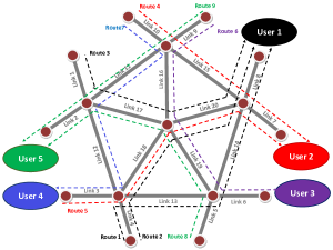
Figure 1: The network

Users have access to different routes as shown in Figure 1. For example, user $1$ can access routes $1$, $2$, and $3$. Each user is characterized by a cost function. Additionally, there is a congestion cost function that depends on the aggregate flow. More specifically, the cost function user $i$ with flow rate (bandwidth) $x_{i}$ is defined by

$$f_{i}(x_{i},\xi_{i})\triangleq-\sum_{r\in\mathcal{R}(i)}\xi_{i}(r)\log(1+x_{i}(r)),$$

for $i=1,\ldots,5$, where $x\triangleq(x_{1};\ldots;x_{5})$ is the flow decision vector of the users, $\xi\triangleq(\xi_{1};\ldots;\xi_{5})$ is a random parameter corresponding to the different users, $\mathcal{R}(i)=\{1,2,\ldots,n_{i}\}$ is the set of routes assigned to the $i$-th user, $x_{i}(r)$ and $\xi_{i}(r)$ are the $r$-th element of the decision vector $x_{i}$ and the random vector $\xi_{i}$, respectively. We assume that $\xi_{i}(r)$ is drawn from a uniform distribution for each $i$ and $r$ and the links have limited capacities given by $b$.

We may define the routing matrix $A$ that describes the relation between set of routes $\mathcal{R}=\{1,2,\ldots,9\}$ and set of links $\mathcal{L}=\{1,2,\ldots,20\}$. Assume that $A_{lr}=1$ if route $r\in\mathcal{R}$ goes through link $l\in\mathcal{L}$ and $A_{lr}=0$ otherwise. Using this matrix, the capacity constraints of the links can be described by $Ax\leq b$.

We formulate this model as a stochastic optimization problem given by

minimize $$\sum_{i=1}^{N}\mathsf{E}\!\left[f_{i}(x_{i},\xi_{i})\right]+c(x)$$ (32)

subject to $$Ax\leq b,\hbox{ and }x\geq 0,$$

where $c(x)$ is the network congestion cost. We consider this cost of the form $c(x)=\|Ax\|^{2}$. Problem (32) is a convex optimization problem and the optimality conditions can be stated as a variational inequality given by $\nabla f(x^{*})^{T}(x-x^{*})\geq 0$, where $f(x)\triangleq\sum_{i=1}^{N}\mathsf{E}\!\left[f_{i}(x_{i},\xi_{i})\right]+c(x)$. Using our notation in Sec. II, we have

$$F(x)=-\left(\frac{\bar{\xi}_{1}(1)}{1+x_{1}(1)};\ldots;\frac{\bar{\xi}_{5}(2)}{1+x_{5}(2)}\right)+2A^{T}Ax,$$

where $\bar{\xi}_{i}(r_{i})\triangleq\mathsf{E}\!\left[\xi_{i}(r_{i})\right]$ for any $i=1,\ldots,5$ and $r_{i}=1,\ldots,n_{i}$. It can be shown that the mapping $F$ is strongly monotone and Lipschitz with specified parameters (cf. [19]). We solve the bandwidth-sharing problem for $12$ different settings of parameters shown in Table I. We consider $4$ parameters in our model that scale the problem. Here, $m_{b}$ denotes the multiplier of the capacity vector $b$, $m_{c}$ denotes the multiplier of the congestion cost function $c(x)$, and $m_{\xi}$ and $d_{\xi}$ are two multipliers that parametrize the random variable $\xi$. $S(i)$ denotes the $i$-th setting of parameters. For each of these $4$ parameters, we consider $3$ settings where one parameter changes and other parameters are fixed. This allows us to observe the sensitivity of the algorithms with respect to each of these parameters.

-	S$(i)$	$m_{b}$	$m_{c}$	$m_{\xi}$	$d_{\xi}$
$m_{b}$	1	1	1	5	2
	2	0.1	1	5	2
	3	0.01	1	5	2
$m_{c}$	4	0.1	2	2	1
	5	0.1	1	2	1
	6	0.1	0.5	2	1
$m_{\xi}$	7	1	1	1	5
	8	1	1	2	5
	9	1	1	5	5
$d_{\xi}$	10	1	0.01	1	1
	11	1	0.01	1	2
	12	1	0.01	1	5

TABLE I: Parameter settings

The SA algorithms are terminated after $4000$ iterates. To measure the error of the schemes, we run each scheme $25$ times and then compute the mean squared error (MSE) using the metric $\frac{1}{25}\sum_{i=1}^{25}\|x_{k}^{i}-x^{*}\|^{2}$ for any $k=1,\ldots,4000$, where $i$ denotes the $i$-th sample. Table II and III show the $90\%$ confidence intervals (CIs) of the error for the DASA and HSA schemes.

-	S$(i)$	DASA - $90\%$ CI	HSA with $\theta=0.1$- $90\%$ CI
$m_{b}$	1	[$2.97$e${-6}$,$4.66$e${-6}$]	[$1.52$e${-6}$,$2.37$e${-6}$]
	2	[$2.97$e${-6}$,$4.66$e${-6}$]	[$1.52$e${-6}$,$2.37$e${-6}$]
	3	[$1.15$e${-7}$,$3.04$e${-7}$]	[$2.12$e${-8}$,$4.92$e${-8}$]
$m_{c}$	4	[$4.39$e${-7}$,$6.55$e${-7}$]	[$1.33$e${-6}$,$1.80$e${-6}$]
	5	[$1.29$e${-6}$,$1.97$e${-6}$]	[$9.00$e${-6}$,$1.20$e${-5}$]
	6	[$3.44$e${-6}$,$5.36$e${-6}$]	[$2.26$e${-4}$,$2.53$e${-4}$]
$m_{\xi}$	7	[$4.29$e${-5}$,$6.40$e${-5}$]	[$7.92$e${-5}$,$1.49$e${-4}$]
	8	[$3.18$e${-5}$,$4.83$e${-5}$]	[$3.46$e${-5}$,$6.07$e${-5}$]
	9	[$1.83$e${-5}$,$2.88$e${-5}$]	[$6.12$e${-6}$,$9.99$e${-6}$]
$d_{\xi}$	10	[$3.82$e${-4}$,$5.91$e${-4}$]	[$2.86$e${+1}$,$2.86$e${+1}$]
	11	[$9.81$e${-4}$,$1.44$e${-3}$]	[$2.86$e${+1}$,$2.86$e${+1}$]
	12	[$6.26$e${-3}$,$8.44$e${-3}$]	[$2.85$e${+1}$,$2.86$e${+1}$]

TABLE II: $90\%$ CIs for DASA and HSA schemes – Part I

-	S$(i)$	HSA with $\theta=1$ - $90\%$ CI	HSA with $\theta=10$ - $90\%$ CI
$m_{b}$	1	[$1.70$e${-6}$,$2.97$e${-6}$]	[$1.33$e${-5}$,$1.81$e${-5}$]
	2	[$1.70$e${-6}$,$2.97$e${-6}$]	[$1.33$e${-5}$,$1.81$e${-5}$]
	3	[$4.66$e${-8}$,$1.17$e${-7}$]	[$8.07$e${-7}$,$2.43$e${-6}$]
$m_{c}$	4	[$4.71$e${-7}$,$8.75$e${-7}$]	[$3.84$e${-6}$,$5.38$e${-6}$]
	5	[$7.88$e${-7}$,$1.36$e${-6}$]	[$5.61$e${-6}$,$7.98$e${-6}$]
	6	[$1.25$e${-6}$,$1.99$e${-6}$]	[$7.34$e${-6}$,$1.12$e${-5}$]
$m_{\xi}$	7	[$2.83$e${-5}$,$4.75$e${-5}$]	[$1.84$e${-4}$,$2.75$e${-4}$]
	8	[$1.97$e${-5}$,$3.39$e${-5}$]	[$1.40$e${-4}$,$1.99$e${-4}$]
	9	[$1.06$e${-5}$,$1.85$e${-5}$]	[$8.33$e${-5}$,$1.13$e${-4}$]
$d_{\xi}$	10	[$5.50$e${-1}$,$5.70$e${-1}$]	[$7.23$e${-5}$,$9.64$e${-5}$]
	11	[$5.45$e${-1}$,$5.85$e${-1}$]	[$2.85$e${-4}$,$3.80$e${-4}$]
	12	[$5.47$e${-1}$,$6.44$e${-1}$]	[$1.77$e${-3}$,$2.36$e${-3}$]

TABLE III: $90\%$ CIs for DASA and HSA schemes – Part II

Insights: We observe that DASA scheme performs favorably and is far more robust in comparison with the HSA schemes with different choice of $\theta$. Importantly, in most of the settings, DASA stands close to the HSA scheme with the minimum MSE. Note that when $\theta=1$ or $\theta=10$, the stepsize $\frac{\theta}{k}$ is not within the interval $(0,\frac{\eta-\beta L}{(1+\beta)^{2}L^{2}}]$ for small $k$ and is not feasible in the sense of Prop. 2. Comparing the performance of each HSA scheme in different settings, we observe that HSA schemes are fairly sensitive to the choice of parameters. For example, HSA with $\theta=0.1$ performs very well in settings S$(1)$, S$(2)$, and S$(3)$, while its performance deteriorates in settings S$(10)$, S$(11)$, and S$(12)$. A similar discussion holds for other two HSA schemes. A good instance of this argument is shown in Figure 2 and 3.

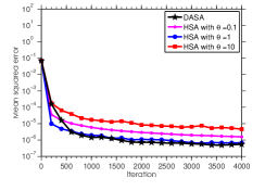
Figure 2: DASA vs. HSA schemes – Setting S($4$)

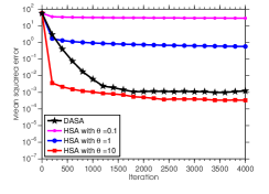
Figure 3: DASA vs. HSA schemes – Setting S($11$)

VI Concluding remarks

We considered distributed monotone stochastic Nash games where each player minimizes a convex function on a closed convex set. We first formulated the problem as a stochastic VI and then showed that under suitable conditions, for a strongly monotone and Lipschitz mapping, the SA scheme guarantees almost-sure convergence to the solution. Next, motivated by the naive stepsize choices of SA algorithm, we proposed a class of distributed adaptive steplength rules where each player can choose his own stepsize independent of the other players from a specified range. We showed that this scheme provides almost-sure convergence and also minimizes a suitably defined error bound of the SA algorithm. Numerical experiments, reported in Section V confirm this conclusion.

References

• [1] F. Yousefian, A. Nedić, and U. V. Shanbhag, “On stochastic gradient and subgradient methods with adaptive steplength sequences,” Automatica, vol. 48, no. 1, pp. 56–67, 2012, an extended version of the paper available at: http://arxiv.org/abs/1105.4549.
• [2] J. Koshal, A. Nedić, and U. V. Shanbhag, “Single timescale regularized stochastic approximation schemes for monotone nash games under uncertainty,” Proceedings of the IEEE Conference on Decision and Control (CDC), pp. 231–236, 2010.
• [3] H. Robbins and S. Monro, “A stochastic approximation method,” Ann. Math. Statistics, vol. 22, pp. 400–407, 1951.
• [4] Y. M. Ermoliev, Stochastic Programming Methods.   Moscow: Nauka, 1976.
• [5] ——, “Stochastic quasigradient methods and their application to system optimization,” Stochastics, vol. 9, pp. 1–36, 1983.
• [6] ——, “Stochastic quasigradient methods,” in Numerical Techniques for Stochastic Optimization.   Sringer-Verlag, 1983, pp. 141–185.
• [7] V. S. Borkar, Stochastic Approximation: A Dynamical Systems Viewpoint.   Cambridge University Press, 2008.
• [8] H. J. Kushner and G. G. Yin, Stochastic Approximation and Recursive Algorithms and Applications.   Springer New York, 2003.
• [9] H. Jiang and H. Xu, “Stochastic approximation approaches to the stochastic variational inequality problem,” IEEE Transactions on Automatic Control, vol. 53, no. 6, pp. 1462–1475, 2008.
• [10] M. Vrahatis, G. Androulakis, J. Lambrinos, and G. Magoulas, “A class of gradient unconstrained minimization algorithms with adaptive stepsize,” Journal of Computational and Applied Mathematics, vol. 114, pp. 367–386, 2000.
• [11] J. C. Spall, “Adaptive stochastic approximation by the simultaneous perturbation method,” IEEE Transactions Automatic Control, vol. 45, no. 10, pp. 1839–1853, 2000.
• [12] D. Cicek, M. Broadie, and A. Zeevi, “General bounds and finite-time performance improvement for the kiefer-wolfowitz stochastic approximation algorithm,” To appear in Operations Research, 2011.
• [13] A. N. S.S. Ram and V. Veeravalli, “Incremental stochastic subgradient algorithms for convex optimization,” SIAM Journal on Optimization, vol. 20, no. 2, pp. 691–717, 2019.
• [14] M. Jimenez-Lizarraga, A. Poznyak, and M. Alcorta, “Leader-follower strategies for a multi-plant differential game,” Proceedings of the American Control Conference, 2008.
• [15] F. Yousefian, A. Nedić, and U. Shanbhag, “A regularized adaptive steplength stochastic approximation scheme for monotone stochastic variational inequalities,” Proceedings of the 2011 Winter Simulation Conference, pp. 4110–4121, 2011.
• [16] B. Polyak, Introduction to optimization.   New York: Optimization Software, Inc., 1987.
• [17] F. Facchinei and J.-S. Pang, Finite-dimensional variational inequalities and complementarity problems. Vols. I,II, ser. Springer Series in Operations Research.   New York: Springer-Verlag, 2003.
• [18] S.-W. Cho and A. Goel, “Bandwidth allocation in networks: a single dual update subroutine for multiple objectives,” Combinatorial and algorithmic aspects of networking, vol. 3405, pp. 28–41, 2005.
• [19] F. Yousefian, A. Nedić, and U. Shanbhag, “Distributed adaptive steplength stochastic approximation schemes for cartesian stochastic variational inequality problems,” Submitted to Mathematical Programming, January 2013.