Probabilistic approach to the length-scale dependence of the effect of water hydrogen bonding on hydrophobic hydration

Abstract.

We present a probabilistic approach to water-water hydrogen bonding that allows one to obtain an analytic expression for the number of bonds per water molecule as a function of both its distance to a hydrophobic particle and hydrophobe radius. This approach can be used in the density functional theory (DFT) and computer simulations to examine particle size effects on the hydration of particles and on their solvent-mediated interaction. For example, it allows one to explicitly identify a water hydrogen bond contribution to the external potential whereto a water molecule is subjected near a hydrophobe. The DFT implementation of the model predicts the hydration free energy per unit area of a spherical hydrophobe to be sharply sensitive to the hydropobe radius for small radii and weakly sensitive thereto for large ones; this corroborates the vision of the hydration of small and large length-scale particles as occurring via different mechanisms. On the other hand, the model predicts that the hydration of even apolar particles of small enough radii may become thermodynamically favorable owing to the interplay of the energies of pairwise (dispersion) water-water and water-hydrophobe interactions. This sheds light on previous counterintuitive observations (both theoretical and simulational) that two inert gas molecules would prefer to form a solvent-separated pair rather than a contact one.

1 Introduction

A particle whereof the accommodation in water is accompanied by an increase in an associated free energy is called “hydrophobic” and is often referred to as a hydrophobe. The thermodynamically unfavorable dissolution of a hydrophobe (whether microscopic or macroscopic) is hydrophobic hydration; the corresponding free increase results from structural (and possibly energetic) changes in water around the hydrophobe. The total volume of water affected by two hydrophobes is smaller when they are close together than when they far away from each other. This gives rise to an effective, solvent-mediated attraction between them which is also referred to as hydrophobic attraction.

Hydrophobic effects (hydration and attraction) play a crucial role in various physical, chemical, and biological phenomena.^1-4 They also play an important role in the formation, stability, and unfolding of the native structure of a biologically active protein which constitute the core of two most exciting (and intrinsically related) topics of modern biophysics, namely, “protein folding” and “protein denaturation”,^5,6 although an assortment of interactions (including those of hydrophilic character⁷) would most likely determine the driving force of these amazing phenomena.

Various mechanisms have been suggested to understand hydrophobic effects at a fundamental level and develop a general theory of hydrophobicity.^8-11 Virtually all theoretical models involve the hydrogen bonding ability of water as a key element.

The structure of liquid water, its dependence on the external conditions, and the role of structural changes in hydrophobic phenomena have long been the subject of intense research. For ambient conditions, it was first described as a locally ordered tetrahedral network of water molecules.¹² Various anomalous properties of water (such as the density maximum at 4^∘ C at atmospheric pressure, local maximum and minimum of the isobaric heat capacity at constant pressure, etc…) are attributed to the ability of its molecules to form hydrogen bonds, strong directional bonds with energy much larger than the thermal energy $k_{B}T$. As an example of water structure effects on hydrophobic phenomena, the biological activity of proteins appears to depend on the formation, maintenance, and breakup of a 2-D hydrogen-bonded network spanning most of the protein surface and connecting all the surface hydrogen-bonded water clusters.¹³

Although much experimental, computational, and theoretical research has been carried out, many thermodynamic and molecular aspects of hydration remain to be clarified. In the positive (unfavorable) free energy of dissolving a hydrophobe, the positive entropic contribution (due to the negative entropy change) dominates over the enthalpic contribution at room temperatures. The total contribution of hydrogen bonding to the hydration enthalpy depends both on the single bond energy and the number of bonds that a water molecule can form in the hydrophobe vicinity and in the bulk. The propensity of water to form all possible hydrogen bonds, on one hand, and the constraint, imposed by a hydrophobe on the configurational space available to vicinal water molecules, on the other hand, lead to a large entropic cost. Some investigations have suggested that water is more structured near a hydrophobe, with water-water hydrogen bonds both labile and stronger than in bulk, but several experimental and theoretical studies have reported the opposite results. Despite remaining controversies, the dependence of hydrophobic phenomena on the length scales of solute particles is considered to be proven.^14-16

The hydration of small hydrophobic molecules (of sizes comparable to a water molecule) is believed to be entropically “driven” (and so is their solvent-mediated interaction).^10,11 Such molecules can fit into the water hydrogen-bond network without destroying any bonds. While this results in a negligible enthalpy of hydration, the solute constrains some degrees of freedom of neighboring water molecules which gives rise to negative hydration entropy and hence to positive hydration free energy. However, such a simple mechanism has recently come under scrutiny^10,11,14,15 because there are simulations^17,18 and theory¹⁹ suggesting that, under some conditions, the hydration of small hydrophobic molecules could be entropically favorable.

The hydration of large hydrophobic particles is believed to occur via a different mechanism.^10,11,19,20 When inserted into liquid water, a large hydrophobe breaks some hydrogen bonds in its vicinity. This would result in large positive hydration enthalpy and hence in a free energy change proportional to the solute surface area (as opposed to being proportional to the solute volume for small hydrophobes). Thus, the hydration of large hydrophobic particles is expected to be enthalpically driven (and so is their solvent-mediated interaction).

As the thermodynamics of hydration is expected to change gradually from entropic for small solutes to enthalpic for large solutes, so are the structural properties of liquid water in the vicinity of the solutes. It was argued²¹ that if the solute-water attraction is sufficiently weak, there may exist a thin film of water vapor near large hydrophobic solutes but not small ones. This generated much controversy.^{10,11,18,20,22}

Hereafter we present a model for water-water hydrogen bonding that allows one to obtain an analytic expression for the number of bonds per water molecule as a function of both its distance to a hydrophobe and hydrophobe radius. This function can be used in the density functional theory (DFT) and computer simulations (either Monte Carlo or Molecular Dynamics) to examine particle size effects on the hydration of particles and on their solvent-mediated interactions over the entire small-to-large length-scale range.

Note that we do not investigate drying or wetting transitions²³ as such; once the accomodation of the solute particle in liquid water occurred, the fluid density distribution in the vicinity of the solute and in the entire system is not subject to any ”transformations”. The latter may be induced only by changes in external thermodynamic variables (either temperature or pressure or chemical potential). We will consider a ”static” version of the hydration phenomenon, wherein the state of the system does not change after hydration occurred.

2 The number of hydrogen bonds per water molecule near a spherical hydrophobic surface

Consider a spherical hydrophobic particle of radius $R$ immersed in liquid water (Figure 1). Even if one assumes that the intrinsic hydrogen bonding ability of a water molecule is not affected by the hydrophobe, in its vicinity a “boundary” water molecule forms a smaller number of bonds than in bulk because the surface restricts the configurational space available to other water molecules necessary for a boundary water molecule to form hydrogen bonds. The probabilistic model allows one to obtain an analytic expression for the average number of bonds that a boundary water molecule can form as a function of its distance to the hydrophobe and hydrophobe radius. A boundary hydrogen bond may be slightly altered energetically compared to the bulk one, but such alteration is still uncertain^24-26 and will be neglected hereafter.

In the probabilistic hydrogen bond (PHB) approach,²⁷ a water molecule is considered to have four arms each capable of forming a single hydrogen bond. The configuration of four hydrogen-bonding (hb) arms is rigid and symmetric (tetrahedral) with the inter-arm angles $\alpha=109.47^{\circ}$ (Fig.1). Each hb-arm can adopt a continuum of orientations subject to the constraint of tetrahedral rigidity. A water molecule can form a hydrogen bond with another molecule only when the tip of any of its hb-arms coincides with the second molecule. The length of a hb-arm thus equals the length of a hydrogen bond $\eta$, assumed independent of whether the molecules are in bulk or near a hydrophobe. The characteristic length of pairwise interactions between water molecules and molecules constituting the hydrophobe is also assumed to be $\eta$.

The location of a water molecule is determined by the distance $r$ from its center to the center of the hydrophobe which is also chosen as the origin of the spherical coordinate system. The distance $x$ between water molecule and hydrophobe is defined as $x=r-R$ (Fig.1).

Denote the number of hydrogen bonds per bulk water molecule by $n_{b}$ and the average number of hydrogen bonds per boundary water molecule by $n_{s}$. The latter is a function of radius $R$ and distance $x$, i.e., $n_{s}\equiv n_{s}(R,x)$. If $x>2\eta$, the number of hydrogen bonds that the water molecule can form is assumed to be unaffected by the hydrophobe: $n_{s}(R,x)=n_{b}$ for $x\geq 2\eta$. On the other hand, the function $n_{s}(R,x)$ attains its minimum at $x=\eta$, because at this distance the configurational space available for neighboring water molecules is most restricted compared to bulk water. A spherical layer of thickness $\eta$ from $r=R+\eta$ to $r=R+2\eta$ is referred to as the solute hydration layer (SHL).

In the spirit of the PHB approach²⁷ let us represent the function $n_{s}=n_{s}(R,x)$ as

$$n_{s}=k_{1}b_{1}+k_{2}b_{1}^{2}+k_{3}b_{1}^{3}+k_{4}b_{1}^{4},$$ (1)

where $b_{1}$ is the probability that one of the hb-arms (of a bulk water molecule) can form a hydrogen bond and the coefficients $k_{1},k_{2},k_{3}$, and $k_{4}$ depend on $R$ and $x$, and so does $n_{s}$. Equation (1) assumes that the intrinsic hydrogen-bonding ability of a water molecule (the tetrahedral configuration of its hb-arms and their lengths and energies) is unaffected by the hydrophobe.

The functions $k_{1}\equiv k_{1}(R,x),k_{2}\equiv k_{2}(R,x),k_{3}\equiv k_{3}(R,x)$, and $k_{4}\equiv k_{4}(R,x)$ can be evaluated by using geometric considerations (see the Appendix). They all become equal to $1$ at $x\geq 2\eta$, where eq.(1) reduces to its bulk analog, $n_{b}=b_{1}+b_{1}^{2}+b_{1}^{3}+b_{1}^{4}$ (see the Appendix). Since experimental data on $n_{b}$ are readily available, one can find $b_{1}$ as a positive solution (satisfying $0<b_{1}<1$) of the latter equation.

Thus, equation (1) provides an efficient pathway to $n_{s}$ as a function of $x$ and $R$. It takes into account the constraint that near the hydrophobe some orientations of the hb-arms of a boundary water molecule cannot lead to the formation of hydrogen bonds. This constraint depends on the distance betwe water molecule and hydrophobe and on the hydrophobe radius, whence the $R$- and $x$-dependence of $k_{1},k_{2},k_{3},$ and $k_{4}$.

Figure 2 presents the function $n_{s}(R,x)$ for a spherical hydrophobe immersed in water at temperature $T=293.15$ K, which corresponds to $n_{b}=3.65$ hence $b_{1}=0.963707$. In Fig.2a, $n_{s}$ is plotted vs $\xi\equiv(x/\eta-1)$ for various radii $R$. As expected,$n_{s}$ monotonically increases from its minimum at $x=\eta$ to its maximum bulk value $n_{b}$ at $x=2\eta$. For a flat hydrophobic surface ($R=\infty$), molecular dynamics simulations^28,29 previously reported such behavior of $n_{s}$ (although with some oscillations in ref.29). In Fig.2b, $n_{s}$ is shown as a function of $R$ at different distances $x$. At any $x$, $n_{s}$ monotonically decreases from its maximum for the smallest particle $R=0$ to its minimum for the largest particle ($R=\infty$). Besides, for any fixed $x$, as $R$ increases from $0$ to $\infty$, $n_{s}$ approaches its asymptotic value for a flat hydrophobic surface, $n_{s}(\infty,x)$, for particles of radii as small as $R\approx 30\eta$.

3 Implementation of the probabilistic hydrogen bond model in the density functional theory

The fluid density distribution near a rigid surface can be efficiently studied by using computer simulations or DFT.^30-32 As an illustration of the PHB approach, let us implement it into DFT. The latter usually treats the interaction of fluid molecules with a foreign (impenetrable) substrate in the mean-field approximation whereby every fluid molecule is considered to be subjected to an external potential, due to its pairwise interactions with the substrate molecules.^31,32 The substrate effect on the ability of fluid (water) molecules to form hydrogen bonds had been previously neglected. However, using the PHB model, one can explicitly implement that effect in the DFT formalism and clarify its role in the length-scale dependence of hydrophobic hydration.

To apply DFT to the thermodynamics of hydrophobic phenomena, it is necessary to know the total external potential field $U_{\mbox{\tiny ext}}^{\mbox{\tiny}}\equiv U_{\mbox{\tiny ext}}^{\mbox{\tiny}}(R,x)$ whereto a water molecule is subjected near a hydrophobic particle. This potential can be written as

$$U_{\mbox{\tiny ext}}=U_{\mbox{\tiny ext}}^{\mbox{\tiny p}}+U_{\mbox{\tiny ext}}^{\mbox{\tiny h}},$$ (2)

where $U_{\mbox{\tiny ext}}^{\mbox{\tiny h}}\equiv U_{\mbox{\tiny ext}}^{\mbox{\tiny h}}(R,x)$ is the water-water hydrogen bond contribution to $U_{\mbox{\tiny ext}}$, and $U_{\mbox{\tiny ext}}^{\mbox{\tiny p}}\equiv U_{\mbox{\tiny ext}}^{\mbox{\tiny p}}(R,x)$ represents the external pairwise potential exerted by all the molecules constituting the hydrophobe on a water molecule.

While various models were designed^31-33 for $U_{\mbox{\tiny ext}}^{\mbox{\tiny p}}$, the hydrogen bond contribution $U_{\mbox{\tiny ext}}^{\mbox{\tiny h}}$ had been conventionally neglected until recently^34,35. This contribution, $U_{\mbox{\mbox{\tiny ext}}}^{\mbox{\tiny h}}$, is due to the deviation of $n_{s}$ from $n_{b}$ as well as the (possible) deviation of $\varepsilon_{s}$ from $\varepsilon_{b}$ (the latter effect is neglected hereafter). It can be determined as

$$U_{\mbox{\tiny ext}}^{\mbox{\tiny h}}=\frac{1}{2}(\varepsilon_{s}n_{s}-\varepsilon_{b}n_{b}).$$ (3)

The first term on the RHS of eq.(3) represents the total energy of hydrogen bonds of a water molecule at a distance $x$ from the surface of a particle of radius $R$, whereas the second term is the energy of its hydrogen bonds in bulk (at $x\rightarrow\infty$); the factor $1/2$ is needed to prevent double counting the energy because every hydrogen bond and its energy, either $\varepsilon_{s}$ or $\varepsilon_{b}$, are shared between two molecules (in refs.34 and 35 the analogous equation for a planar surface was mistyped, as the factor $1/2$ was missing). Note that $U_{\mbox{\tiny ext}}^{\mbox{\tiny h}}(R,x)\neq 0$ only for $\eta\leq x\leq 2\eta$.

In DFT, the grand thermodynamic potential $\Omega$ of a nonuniform single component fluid, subjected to an external potential $U_{\mbox{\tiny ext}}$ (representing the hydrophobe), is a functional of the number density $\rho(\bf{r})$ of fluid molecules

$$\Omega[\rho(\bf{r})] = \mathcal{F}_{\mbox{\tiny h}}[\rho({\bf r})]+\frac{1}{2}\int\int d{\bf r}d{\bf r^{\prime}}\,\rho({\bf r})\rho({\bf r^{\prime}})\phi_{\mbox{\tiny at}}(|\bf{r}-\bf{r^{\prime}}|)$$ (4)

$$+ \int d{\bf r}\,U_{\mbox{\tiny ext}}({R,\bf r})\rho({\bf r})-\mu\int d{\bf r}\,\rho({\bf r}),$$

where $\mathcal{F}_{\mbox{\tiny h}}[\rho({\bf r})]$ is the intrinsic Helmholtz free energy functional of hard sphere fluid, $\mu$ is the chemical potential, and $\phi_{\mbox{\tiny at}}(|\bf{r}-\bf{r^{\prime}}|)$ is the attractive part of the interaction potential between two fluid molecules located at ${\bf r}$ and ${\bf r^{\prime}}$; the integrals are taken over the volume $V$ of the system. Among various models for $\mathcal{F}_{\mbox{\tiny h}}[\rho({\bf r})]$, the weighted density approximation (WDA)^30,36,37 with a weight function independent of weighted density represents an optimal combination of accuracy and simplicity. It is non-local with respect to $\rho({\bf r})$; it takes into account short-ranged correlations and captures the fluid density oscillations near a hard wall. We hereafter adopt the WDA version of DFT.

The key element of WDA is the weighted density $\widetilde{\rho}({\bf r})$ determined in terms of $\rho({\bf r})$ via an implicit equation

$$\widetilde{\rho}({\bf r})=\int d{\bf r^{\prime}}\,\rho({\bf r^{\prime}})w(|{\bf r^{\prime}}-{\bf r}|;\widetilde{\rho}({\bf r})),$$ (5)

where $w(|{\bf r^{\prime}}-{\bf r}|;\widetilde{\rho}({\bf r}))$ is the weight function. Although in more sophisticated versions^30,36 of WDA $w(|{\bf r^{\prime}}-{\bf r}|;\widetilde{\rho}({\bf r}))$ depends on $\widetilde{\rho}({\bf r})$, we will hereafter adopt its simpler version wherein the weight function is independent^30,37 of $\widetilde{\rho}({\bf r})$.

For hydrophobic hydration in an open system of constant $\mu$, $V$, and $T$ (grand canonical ensemble), the equilibrium density profile is obtained by minimizing $\Omega[\rho(\bf{r})]$ with respect to $\rho({\bf r})$. The corresponding Euler-Lagrange equation can be written as

$$\mu=k_{B}T\ln(\Lambda^{3}\rho({\bf r}))+W({\bf r};\rho({\bf r})),$$ (6)

where $\Lambda=(h^{2}/2\pi mk_{B}T)^{1/2}$ is the thermal de Broglie wavelength of a molecule of mass $m$ ($h$ and $k_{B}$ being Planck’s and Boltzmann’s constants) and $W({\bf r};\rho({\bf r}))$ is a function of ${\bf r}$ and a functional of $\rho({\bf r})$:^28-30

$$W({\bf r};\rho({\bf r})) = U_{\mbox{\tiny ext}}({\bf r})+\int d{\bf r^{\prime}}\,\rho({\bf r^{\prime}})\phi_{\mbox{\tiny a}}(|{\bf r}-{\bf r^{\prime}}|)$$ (7)

$$+ \Delta\psi_{\mbox{\tiny h}}(\widetilde{\rho}({\bf r}))+\int d{\bf r^{\prime}}\,\rho({\bf r^{\prime}})\,\Delta\psi^{\prime}_{\mbox{\tiny h}}(\widetilde{\rho}({\bf r^{\prime}}))w(|{\bf r^{\prime}}-{\bf r}|).$$

Here $\phi_{\mbox{\tiny a}}(|{\bf r}-\bf{r^{\prime}}|)$ is the attractive part of the interaction potential between two fluid molecules located at ${\bf r}$ and ${\bf r^{\prime}}$, whereas $\Delta\psi_{\mbox{\tiny h}}(\rho)$ is the configurational part of the free energy of hard sphere fluid per molecule, with $\Delta\psi^{\prime}_{\mbox{\tiny h}}(\rho)\equiv d\Delta\psi_{\mbox{\tiny h}}(\rho)/d\rho$.

The hydrophobe being spherical, the external potential is a function of a single variable $x=r-R$, and the equilibrium density profile obtained from eq.(6) is a function of a single variable $r$: $\rho({\bf r})=\rho(r)$. The substitution of $\rho(r)$ into eq.(4) provides the grand thermodynamic potential $\Omega$ of the non-uniform fluid with a hydrophobe therein. The grand canonical free energy of hydration is $\Delta\Omega_{\mbox{\tiny}}=\Omega-\Omega_{0}$, where $\Omega_{0}$ is the grand thermodynamic potential of uniform liquid water without a hydrophobe therein.

4 Numerical Calculations

For a numerical illustration, we considered the hydration of a spherical hydrophobe (taking $R/\eta=1,3,5,7,10,15,20,30,50,100$) in the model water at $T=293.15$ K and $\mu=-11.5989$ $k_{B}T$ corresponding to its two-phase equilibrium. The liquid state of bulk water was ensured by imposing the appropriate boundary condition onto eq.(6), $\rho(x)\rightarrow\rho_{l}$ as $x\rightarrow\infty$, with $\rho_{l}$ the bulk liquid density. The densities $\rho_{v}$ and $\rho_{l}$ of coexisting vapor and liquid, respectively, are determined by solving the equations $\left.\mu(\rho,T)\right|_{\rho=\rho_{v}}=\left.\mu(\rho,T)\right|_{\rho=\rho_{l}},\;\;\;\;\;\;\;\;\left.p(\rho,T)\right|_{\rho=\rho_{v}}=\left.p(\rho,T)\right|_{\rho=\rho_{l}}$, requiring the chemical potential $\mu\equiv\mu(\rho,T)$ and pressure $p\equiv p(\rho,T)$ to be the same throughout both coexisting phases.

The chemical potential of a uniform hard sphere fluid $\mu_{\mbox{\tiny h}}$ and the configurational part $\Delta\psi_{\mbox{\tiny h}}\equiv\Delta\psi_{\mbox{\tiny h}}(\rho,T)$ of the free energy of a hard sphere fluid were modeled in the Carnahan-Starling approximation,^31,32,38 whereas for the weight function $w(|{\bf r^{\prime}}-{\bf r}|;\widetilde{\rho}({\bf r}))$ in eqs.(5),(7) we adopted a $\widetilde{\rho}$-independent version³⁷

$$\Delta\psi_{\mbox{\tiny h}}=k_{B}T\frac{\xi\,(4-3\xi)}{(1-\xi)^{2}},\;\;\;\;\;w(r_{12})=\frac{3}{\pi\eta^{4}}(\eta-r_{12})\Theta(\eta-r_{12}),$$

with $\Theta(u)$ being the Heaviside (unit-step) function.

The pairwise interactions of water molecules were modeled by using the Lennard-Jones (LJ) potential with the energy parameter $\varepsilon_{\mbox{\tiny ww}}=3.79\times 10^{-14}$ erg and the diameter $d$ of a model molecule set to be $\eta$. The attractive part $\phi_{\mbox{\tiny at}}$ of pairwise water-water interactions was modeled via the Weeks-Chandler-Anderson perturbation scheme.³⁹ The interaction potential between water molecule and molecule of a hydrophobe was assumed to be of LJ type with an energy parameter $\varepsilon_{\mbox{\tiny wp}}$ and a length parameter $\eta$. Integrating this interaction with respect to the position of the molecule of the hydrophobe over the hydrophobe volume $V_{R}=4\pi R^{3}/3$, one can obtain the pairwise contribution $U_{\mbox{\tiny ext}}^{\mbox{\tiny p}}$ into $U_{\mbox{\tiny ext}}$. We assumed the dimensionless number density of molecules in the hydrophobe to be $\rho_{p}\eta^{3}\approx 1$ and considered five values for $\varepsilon_{\mbox{\tiny wp}}/\varepsilon_{\mbox{\tiny ww}}$ (0.6, 0.66, 0.75, 0.9, 1.2) to mimic various degrees of hydrophobicity. The density profiles and free energies of hydration thus obtained are shown in Figures 3-5.

Figure 3 presents the density profiles near a spherical hydrophobe of radius $R$ for $R/\eta=1,3,5,7,10,15,30,100$ and $\varepsilon_{\mbox{\tiny wp}}/\varepsilon_{\mbox{\tiny ww}}=0.75$ . The profiles in this Figure (as well as in Figure 4) are presented in a coordinate system with the origin $r=0$ located in the center of the hydrophobe; there are no water molecules at $r<R+\eta$ (the space $0<r\leq R$ is occupied by the hydrophobic sphere and the layer $R<r<R+\eta$ is excluded to fluid molecules).As clear, the hydrophobe radius greatly affects the distribution of vicinal water molecules. The oscillations in the density profile gradually disappear as $R$ increases. They are well pronounced for $R/\eta=1$, but virtually non-existent for particles $R/\eta\geq 7$. As $R$ increases, a thin depletion layer around the particle (virtually non-existent for $R/\eta=1$) becomes more developed, with its density approaching that of vapor and its thickness approaching $\eta$.

This is consistent with the largely accepted wisdom concerning the much discussed issue whether or not there is a vapor-like layer near a large hydrophobe in liquid water. As now widely agreed upon, even if (and when) such a layer exists, it should be expected to be of molecular thickness only.^{10,11,19,21-23}

Furthermore, the behavior of fluid density profiles in Fig.3 is consistent with our previous finding^34,35 that the hydrogen bond contribution to the external potential plays a crucial role in the formation of a thin “strong depletion” layer (of density much lower than liquid and of thickness of a molecular diameter) between liquid water and planar hydrophobic surface even for weakly hydrophobic surfaces (with high $\varepsilon_{\mbox{\tiny wp}}/\varepsilon_{\mbox{\tiny ww}}$). Indeed, as $R$ increases, the geometric constraint on the ability of a vicinal water molecule to form hydrogen bonds strengthens, the repulsive contribution $U_{\mbox{\tiny ext}}^{\mbox{\tiny h}}$ to $U_{\mbox{\tiny ext}}$ increases, whence the widening and stronger depletion of the vicinal water layer around the hydrophobe if the “pairwise” hydrophobe-water (attractive) contribution $U_{\mbox{\tiny ext}}^{\mbox{\tiny p}}$ (determined by the ratio $\varepsilon_{\mbox{\tiny wp}}/\varepsilon_{\mbox{\tiny ww}}$) is not too large (by absolute value).

In order to further clarify the effects of water-hydrophobe attraction and hydrophobe radius on fluid (water) density profiles, they are plotted in Figure 4 for three different values of $\varepsilon_{\mbox{\tiny wp}}/\varepsilon_{\mbox{\tiny ww}}$ and two different radii $R$, namely, $R/\eta=1$ (Fig.4a) and $R/\eta=15$ (Fig.4b). Three profiles shown in each of Figs.4a and 4b correspond to $\varepsilon_{\mbox{\tiny wp}}/\varepsilon_{\mbox{\tiny ww}}=0.6,0.75,1.2$ (from bottom to top, respectively). As clear, the strengthening of pairwise intermolecular fluid-hydrophobe interactions by 100% has a little effect on density profiles near a sufficiently large hydrophobe ($R/\eta=15$); the thickness of the depletion layer remains virtually unaffected (roughly equal to $\eta$) and the fluid density therein remains several orders of magnitude lower than its bulk value (i.e., the depletion layer remains vapor-like). On the other hand, for a molecular size hydrophobe ($R/\eta=1$), the increase of $\varepsilon_{\mbox{\tiny wp}}/\varepsilon_{\mbox{\tiny ww}}$ by 100% leads to a drastic change in the nature of the water depletion layer near the hydrophobe; it becomes significantly narrower and from being a vapor-like one transforms into a liquid-like one. These results are in qualitative agreement with the previously reported ones obtained via molecular dynamics simulations⁴⁰ of the SPCE water model and via Monte Carlo simulations⁴¹ of the TIP4P water model. The latter study also reported the analogous behavior for all fluids, including nonassociating ones (without hydrogen-bonding ability). That is somewhat dissimilar from our previous studies³⁴ showing that that even for a relatively strong hydrophobic planar surface (with low $\varepsilon_{\mbox{\tiny wp}}/\varepsilon_{\mbox{\tiny ww}}$) the conventional contribution to the external potential (due to pairwise interactions between a water molecule and those of the substrate) cannot cause the formation of a vapor-like layer near the surface, although it does lead to the formation of a depletion layer with a weak decrease in the vicinal fluid density compared to the bulk one.

In the framework of the proposed approach, the thickness of and the density in the depletion layer are determined by the interplay of two effects. On one hand, the constraint on the configurational space available to water molecules, wherewith a selected molecule can form hydrogen bonds, is taken account of via the function $n_{s}(R,x)$, eq.(1). On the other hand, the model incorporates attractive interactions between water molecule and hydrophobe, eq.(2), whereof the strength can be characterised by the positive parameter $\varepsilon_{\mbox{\tiny wp}}$. For a given thermodynamic state of the system and the nature of the hydrophobe (represented by $\varepsilon_{\mbox{\tiny wp}}$), the result of this interplay naturally depends on the hydrophobe size (radius). When the former effect predominates over the latter, the depletion layer is vapor-like. Otherwise, for relatively weakly hydrophobic particles (that are not too large), the vicinal water layer is just slightly depleted compared to the bulk liquid.

Figure 5a presents the grand canonical free energy of hydrophobic hydration $\Delta\Omega_{\mbox{\tiny}}$ as a function of the hydrophobe radius $R$ (note that the curves are provided only for guiding the eye; the actual calculated points are at $R/\eta=1,3,5,7,10,15,20,30,50$, and $100$). The intrinsic hydrophobicity of the particles is assumed to be independent of $R$, with $\varepsilon_{\mbox{\tiny wp}}/\varepsilon_{\mbox{\tiny ww}}=0.75$. The hydration free energy is expressed in units of $k_{B}T$ per “dimensionless unit area”; the dimensionless $\overline{\Delta\Omega}$ in Figure 4 is obtained by dividing $\Delta\Omega$ by $k_{B}T$ and by $4\pi R^{2}/\eta^{2}$. The variable sensitivity of $\overline{\Delta\Omega}$ to $R$ is a clear indication that the hydration of small and large length-scale particles occurs via different mechanisms and that the hydrogen bond contribution to $U_{\mbox{\tiny ext}}$ plays a key role in this process. The model predictions for $\overline{\Delta\Omega}$ for small $R$’s are consistent with the experimental data on the hydration free energy of methane, ethane, propane, and $n$-butane at the temperature $T=300$ K, as compiled in ref.8; considering a methane molecule as a sphere and ethane, propane, and n-butane molecules as cylinders, one can roughly estimate the experimental $\overline{\Delta\Omega}_{\mbox{\tiny}}$ to be $0.6$ for methane, $0.4$ for ethane, and $0.3$ for propane and $n$-butane.

The dominant role of the hydrogen bond network in hydrophobic hydration is emphasized in Figure 5b where $\overline{\Delta\Omega}$ is plotted vs $\varepsilon_{\mbox{\tiny wp}}/\varepsilon_{\mbox{\tiny ww}}$ for various radii $R$. Each curve in Fig.5b corresponds to a fixed $R$, with $R/\eta=1,3,7,15,30$ from bottom to top (again the curves are provided only for guiding the eye; the actual calculated points are at $\varepsilon_{\mbox{\tiny wp}}/\varepsilon_{\mbox{\tiny ww}}=0.6,0.66,0.75,0.9$, and $1.2$). As expected, the hydration free energy per unit area decreases with increasing degree of hydrophobicity and, for small enough particles, $\overline{\Delta\Omega}$ may even become negative. The model predictions suggest that the hydration of even apolar particles of radii $R\lesssim 3\eta$ may be thermodynamically favorable (the hydration free energy being negative) if the pairwise (LJ-type) interactions between a water molecule and a molecule constituting the hydrophobe are comparable with or stronger than the (LJ-type) interactions between two water molecules, i.e., if $\varepsilon_{\mbox{\tiny wp}}/\varepsilon_{\mbox{\tiny ww}}\gtrsim 1$. This result clarifies some previous simulational and theoretical observations^18-20 that two inert gas molecules would prefer to form a solvent-separated pair rather than a contact pair (dimer).

5 Conclusions

Concluding, we emphasize that the PHB approach allows one to obtain an analytic expression for the average number of hydrogen bonds per water molecule near a spherical hydrophobic particle as a function of both the particle radius and the distance between water molecule and hydrophobe surface. This function can serve as a foundation for elucidating various aspects of hydrophobic phenomena, particularly their length-scale dependence, either via computer simulations (Monte Carlo and Molecular Dynamics) or DFT. For example, this function allows one to explicitly identify an additional contribution to the external potential exerted by the hydrophobe on a water molecule; it is due to the alteration of water hydrogen bonding near a hydrophobe. Thus, one can efficiently implement the hydrogen bonding ability of water molecules in DFT to examine the particle size dependence of hydrophobic hydration.

As a numerical illustration of the combined PHB/DFT approach, we have studied the hydration of spherical particles of various radii and various hydrophobicity in a model water. The numerical results for the hydration free energy of small size hydrophobes are consistent with the experimental data on the hydration of small alkanes. The free energy of hydration per unit area of a spherical particles is predicted to have a varying sensitivity to the particle radius which is a clear indication that the hydration of small and large length-scale particles occurs via different mechanisms. On the other hand, the model predictions suggest that the hydration of even apolar particles of small enough radii may be thermodynamically favorable if the pairwise (dispersion) attraction between a water molecule and a molecule constituting the hydrophobe is comparable with or stronger than the pairwise (dispersion) attractions between two water molecules. This result at least partially clarifies some previous simulational and theoretical observations (rather counterintuitive from the conventional point of view on hydrophobicity) that two inert gas molecules would prefer to form a solvent-separated pair rather than a contact pair (dimer).

Note that in the PHB approach the tetrahedral rigidity (both geometric and energetic) of the hb-arms of a water molecule is assumed only for the analytical simplicity. It can be eliminated to allow for the geometric deformation and energetic alteration of this configuration depending on the sequence in which the hb-arms are engaged or due to the proximity of the water molecule to the hydrophobe. These modifications will just render the model more complicated for analytical treatment and can be expected to relatively weakly affect the model predictions.

Appendix. Derivation of the coefficients $k_{1},k_{2},k_{3}$, and $k_{4}$ as functions of $R$ and $x$

To find the function $n_{s}(R,x)$, first consider its bulk analog, $n_{b}$, and represent it as (see ref.[27] in the main text)

$$n_{b}=b_{1}+b_{2(1)}+b_{3(2,1)}+b_{4(3,2,1)},$$ (A1)

where $b_{1}$ is the probability that one of the hb-arms (of a bulk water molecule) can form a hydrogen bond, $b_{2(1)}$ is the probability that a second hb-arm can form a hydrogen bond subject to the condition that one of the hb-arms has already formed a bond, $b_{3(2,1)}$ is the probability that a third hb-arm can form a hydrogen bond subject to the condition that two of the hb-arms have already formed bonds, and $b_{4(3,2,1)}$ is the probability that the fourth hb-arm can form a bond subject to the condition that three of the hb-arms have already formed bonds.

Note that the probability $b_{1}$ can be formally represented as a product $b_{1}=P_{S\rightarrow N}P_{N\rightarrow S}$, where $P_{S\rightarrow N}$ is the probability that the tip of any hb-arm of molecule $S$ roughly coincides with molecule $N$ and $P_{N\rightarrow S}$ is the probability that the tip of any hb-arm of molecule $N$ roughly coincides with molecule $S$. (Similar considerations are valid for $b_{2(1)},\;b_{3(2,1)}$, and $b_{4(3,2,1)}$ as well). Neither $P_{S\rightarrow N}$ nor $P_{S\rightarrow S}$ can be found in the framework of our simple model, but their product (i.e., $b_{1}$) can be determined from readily available experimental and simulational data on $n_{b}$.

Indeed, in the chosen model of a water molecule the events of formation of bonds by the hb-arms (in bulk water) can be considered as independent of each other, so that $b_{2(1)}=b_{1}^{2},\;\;b_{3(2,1)}=b_{1}^{3},\;\;b_{4(3,2,1)}=b_{1}^{4}.$ Thus, the probability $b_{1}$ can be evaluated as the positive solution of the equation $n_{b}=b_{1}+b_{1}^{2}+b_{1}^{3}+b_{1}^{4}$ satisfying the condition $0<b_{1}<1$. The latter representation of $n_{b}$ implies that the intrinsic hydrogen bonding ability of each arm is independent of whether the other arms have been already engaged in hydrogen bonds or not. That is, when the first hb-arm of a water molecule forms an actual bond, the electron density distribution in a water molecule determining the ability of the other three hb-arms (that are not engaged yet) to form bonds (and their potential orientations) remains unaffected (there is no issue with the availability of water molecules necessary for the selected bulk molecule to form bonds).

For a boundary water molecule, let us represent $n_{s}$ in a form:

$$n_{s}=s_{1}+s_{2(1)}+s_{3(2,1)}+s_{4(3,2,1)}.$$ (A2)

Here $s_{1}\equiv s_{1}(R,x),\;s_{2(1)}\equiv s_{2(1)}(R,x),\;s_{3(2,1)}\equiv s_{3(2,1)}(R,x),\;s_{4(3,2,1)}\equiv s_{4(3,2,1)}(R,x)$ are probabilities analogous to $b_{1},b_{2(1)},b_{3(2,1)},b_{4(3,2,1)}$ subject to the constraint that some orientations of the hb-arms cannot lead to the formation of hydrogen bonds because of the proximity to the hydrophobic particle. The severity of this constraint depends on the distance of the water molecule to the particle, hence the $x^{\prime}$-dependence of $s_{1},s_{2(1)},s_{3(2,1)},s_{4(3,2,1)}$. Again, as a first approximation the intrinsic hydrogen-bonding ability of a water molecule (i.e., the tetrahedral configuration of its hb-arms and their lengths and energies) can be considered to be unaffected by its proximity to the hydrophobic particle so that the latter only restricts the configurational space available to other water molecules necessary for this boundary water molecule to form hydrogen bonds. Thus, one can relate $s_{1},s_{2(1)},s_{3(2,1)}$, and $s_{4(3,2,1)}$ to $b_{1},\;\;b_{2(1)},\;\;b_{3(2,1)}$, and $b_{4(3,2,1)}$, respectively, as

$$s_{1}=k_{1}b_{1},\;\;\;s_{2(1)}=k_{2}b_{2(1)},\;\;\;s_{3(2,1)}=k_{3}b_{3(2,1)},\;\;\;s_{4(3,2,1)}=k_{4}b_{4(3,2,1)},$$ (A3)

where the coefficients $k_{1},\;k_{2},\;k_{3}$, and $k_{4}$ are functions of $R$ and $x$ (with their dependence on the boundary water molecule orientations averaged) and can be evaluated by using geometric considerations.

Coefficient $k_{1}$

The coefficient $k_{1}$ is calculated by taking into account that a boundary water molecule can form a hydrogen bond “almost” like a bulk molecule except for the constraint that the tip of the hb-arm (arm 1) must not be too close to the surface of the hydrophobic particle of radius $R$. Select an arbitrary water molecule at a distance $\eta\leq x\leq 2\eta$ from that surface and denote it $S$ (Figure 4). Any of its hb-arms can form a hydrogen bond if the tip of the arm is located anywhere on a sphere of radius $\eta$ (centered at $S$) from which a spherical cap is cut out by the sphere $ib$ of radius $R+\eta$, inner boundary of the SHL of particle $R$. Denoting the corresponding solid angle by $\Omega_{s}(R,x)$, one can write

$$\Omega_{s}(R,x)=2\pi\int_{0}^{\Theta_{1x}^{M}(x)}d\Theta_{1}\,\sin(\Theta_{1}),$$ (A4)

where $\Theta_{1}$ is the angle between hb-arm 1 and radial axis $r$ (with the origin in the center of the hydrophobe and passing through the molecule $S$), with $\Theta_{1x}^{M}(R,x)\equiv\arccos[-(2(R+\eta+x)+\eta^{2}+x^{2})/2(R+\eta+x)\eta]$ is the maximum angle $\Theta_{1}$ at which hb-arm 1 can still form a bond. The probability $s_{1}(R,x)$ that any one of hb-arms of molecule $S$ can form a hydrogen bond is related to $b_{1}$ via

$$s_{1}(R,x)=\frac{\Omega_{s}(R,x)}{\Omega_{b}}b_{1},$$ (A5)

where $\Omega_{b}=4\pi$. Integrating the RHS of eq.(S4), substituting the result into eq.(S5), and taking into account eq.(S3), one obtains the coefficient $k_{1}\equiv k_{1}(R,x)$ to be :

$$k_{1}=\frac{1}{2}\left(1+\frac{(2(R+\eta)x+\eta^{2}+x^{2})}{2(R+\eta+x)\eta}\right).$$ (A6)

Coefficient $k_{2}$

The coefficient $k_{2}$ is calculated by assuming that hb-arm 1 has already formed a bond in an arbitrary orientation $\Theta_{1}$ (with respect to the radial axis $r$) and by taking into account that hb-arm 2 can form a bond subject to the condition that its tip must not lie closer to the particle surface than the SHL inner boundary $ib$ of hydrophobe $R$.

For a bulk water molecule the probability $b_{2(1)}$, that the second hydrogen bond forms once the first one has formed is proportional to the full length $L_{b}$ of the circle $C_{2}(1)$ formed by the possible loci of the tip of the engaged second hb-arm (hb-arm 2) subject to the restriction that the angle between the two hb-arms remains $\alpha$. Since the radius of that circle is equal to $R_{\mbox{\tiny{C}}_{2(1)}}=\eta\sin(\alpha)$, we have

$$L_{b}=2\pi\eta\sin(\alpha).$$ (A7)

However, for the molecule $S$ the possible loci of the tip of engaged hb-arm 2 (subject to the restriction that the angle between it and hb-arm 1 is $\alpha$) constitute just a part of the circle of radius $\eta\sin(\alpha)$, - the other part (a circular arc) being excluded by the proximity of the SHL inner boundary $ib$. The length of the “available” part of this circle is a function of $R,\,x$, and $\Theta_{1}$ and will be denoted by $L_{s}\equiv L_{s}(R,x,\Theta_{1})$ (by definition, $L_{s}(R,x,\Theta_{1})=L_{b}$ for $x\geq 2\eta$). The probability $s^{\prime}_{2(1)}$ that molecule $S$ engages in a second hydrogen bond once its hb-arm 1 has already formed a bond (at given $R,x,\Theta_{1}$) is proportional to $L_{s}$:

$$s^{\prime}_{2(1)}\equiv s^{\prime}_{2(1)}(R,x,\Theta_{1})=\frac{L_{s}(R,x,\Theta_{1})}{L_{b}}b_{2(1)}$$ (A8)

Let us introduce the Cartesian coordinate system with the origin $O$ in the center of particle $R$, axis $z$ coinciding with the radial axis $r$, and axis $y$ directed from the origin towards the projection of the tip of hb-arm $1$ onto the $x-y$ plane. Depending on the angle $\Theta_{1}$, distance $x$, and radius $R$, the circle $C_{2}(1)$ may either intersect the SHL inner boundary (which is a sphere of radius $R+\eta$ centered at $0$, hereafter denoted $S_{SHL}^{ib}$) or not. In the former case, there may be either two intersection points which can degenerate into one point in the limiting at some particular orientation for given $R$ and $x$. Assuming that there are two intersection points of sphere $S_{SHL}^{ib}$ and circle $C_{2}(1)$, let us denote their Cartesian coordinates by $x_{-},y_{-},z_{-}$ and $x_{+},y_{+},z_{+}$. Clearly, $y_{\pm}\equiv y_{-}=y_{+}$, $z_{\pm}\equiv z_{-}=z_{+}$, and $x_{-}=-x_{+}$; one can choose the notation so that $x_{+}>0$; clearly the coordinates of both points are functions of $R,x,\Theta_{1}$.

Further, let us define the angle $\Theta_{10}(R,x)$ to be the value of the angle $\Theta_{1}$ at which the circle $C_{2}(1)$ just “touches” the sphere $S_{SHL}^{ib}$, and introduce $x^{0}\equiv x^{0}(R)$ and $R^{0}$ as the solutions of equations $\Theta_{10}(R,x^{0})=0$ (with respect to $x^{0}$) and $x^{0}(R^{0})=0$ (with respect to $R^{0}$), respectively. One can thus obtain $R^{0}\approx 0.50009$,

$$x^{0}=-R-\eta\cos(\alpha)+\sqrt{R^{2}+2R\eta+\eta^{2}\cos^{2}(\alpha)},\;\;\;\Theta_{10}(R,x)=-\alpha+\Theta_{1x}^{M}(R,x),$$ (A9)

For $0\leq R<R^{0}$, one can show that

$$L_{s}=\left\{\begin{array}[]{ll}L_{b}&\;\;\;\;\;\;\mbox{if}\;\;\;\;\;\;\Theta_{1}\in\;\;[0;\Theta_{10}(R,x)]\\ L_{c}^{\pm}&\;\;\;\;\;\;\mbox{if}\;\;\;\;\;\;\Theta_{1}\in\;\;\;]\Theta_{10}(R,x);\Theta_{1}^{\mbox{\tiny{mM}}}(R,x)]\\ L_{b}&\;\;\;\;\;\;\mbox{if}\;\;\;\;\;\;\Theta_{1}\in\;\;\;]\Theta_{1}^{\mbox{\tiny{mM}}}(R,x);\Theta_{1x}^{M}(R,x)]\end{array}\right.$$ (A10)

where $\Theta_{1x}^{\mbox{\tiny{mM}}}(R,x)=\min[\Theta_{1x}^{m}(R,x),\Theta_{1x}^{M}(R,x)]$, $\Theta_{1x}^{m}(R,x)=2\pi-\alpha-\Theta_{1x}^{M}(R,x)$, and

$$L_{c}^{\pm}=\left\{\begin{array}[]{ll}2\phi_{\mbox{\tiny{C}}}^{\pm}R_{\mbox{\tiny{C}}_{2(1)}}&\;\;\;\;\;\;\mbox{if}\;\;\;\;\;\;y_{\pm}\geq y_{\mbox{\tiny{C}}_{2(1)}}^{o},\\ 2(\pi-\phi_{\mbox{\tiny{C}}}^{\pm})R_{\mbox{\tiny{C}}_{2(1)}}&\;\;\;\;\;\;\mbox{if}\;\;\;\;\;\;y_{\pm}<y_{\mbox{\tiny{C}}_{2(1)}}^{o},\end{array}\right.$$ (A11)

with $\phi_{\mbox{\tiny{C}}}^{\pm}=\arcsin(x_{+}/\eta\sin(\alpha))$ and $y_{\mbox{\tiny{C}}_{2(1)}}^{o}$ the $y$-coordinate of the center of the circle $C_{2}(1)$. The expression for $L_{c}^{\pm}$ can be also written as

$$L_{c}^{\pm}=\left\{\begin{array}[]{ll}2\phi_{\mbox{\tiny{C}}}^{\pm}R_{\mbox{\tiny{C}}_{2(1)}}&\;\;\;\;\;\;\mbox{if}\;\;\;\;\;\;\Theta_{1}\in\;\;\;[\Theta_{1n}(R,x);\Theta_{1}^{\mbox{\tiny{$\phi$}}}(R,x)],\\ 2(\pi-\phi_{\mbox{\tiny{C}}}^{\pm})R_{\mbox{\tiny{C}}_{2(1)}}&\;\;\;\;\;\;\mbox{if}\;\;\;\;\;\;\Theta_{1}\in\;\;\;]\Theta_{1}^{\mbox{\tiny{$\phi$}}}(R,x);\Theta_{1x}^{\mbox{\tiny{mM}}}(R,x)],\end{array}\right.$$ (A12)

where $\Theta_{1}^{\mbox{\tiny{$\phi$}}}(R,x)$ is the value of the angle $\Theta_{1}$ at which $x_{+}=R_{\mbox{\tiny{C}}_{2(1)}}$.

Considering $R^{0}\leq R<\infty$ one can show that for $x\in[1;x^{0}(R)]$

$$L_{s}=\left\{\begin{array}[]{ll}0&\;\;\;\;\;\;\mbox{if}\;\;\;\;\;\;\Theta_{1}\in\;\;[0;\Theta_{1n}^{\mbox{\tiny{}}}(R,x)],\\ L_{c}^{\pm}&\;\;\;\;\;\;\mbox{if}\;\;\;\;\;\;\Theta_{1}\in\;\;\;]\Theta_{1n}(R,x);\Theta_{1x}^{\mbox{\tiny{mM}}}(R,x)],\\ L_{b}&\;\;\;\;\;\;\mbox{if}\;\;\;\;\;\;\Theta_{1}\in\;\;\;]\Theta_{1x}^{\mbox{\tiny{mM}}}(R,x);\Theta_{1x}^{M}(R,x)],\end{array}\right.$$ (A13)

with $\Theta_{1n}(R,x)=\alpha-\Theta_{1x}^{M}(R,x)$, whereas for $x\in[x^{0}(R);2\eta]$

$$L_{s}=\left\{\begin{array}[]{ll}L_{b}&\;\;\;\;\;\;\mbox{if}\;\;\;\;\;\;\Theta_{1}\in\;\;[0;\Theta_{10}(R,x)],\\ L_{c}^{\pm}&\;\;\;\;\;\;\mbox{if}\;\;\;\;\;\;\Theta_{1}\in\;\;\;]\Theta_{10}(R,x);\Theta_{1x}^{\mbox{\tiny{mM}}}(R,x)],\\ L_{b}&\;\;\;\;\;\;\mbox{if}\;\;\;\;\;\;\Theta_{1}\in\;\;\;]\Theta_{1x}^{\mbox{\tiny{mM}}}(R,x);\Theta_{1x}^{M}(R,x)].\end{array}\right.$$ (A14)

The probability $s_{2(1)}\equiv s_{2(1)}(R,x)$ defined by eq.(S2), can be obtained by integrating $s^{\prime}_{2(1)}(R,x,\Theta_{1})$ with respect to the angle $\Theta_{1}$ subject to the constraint that hb-arm 1 has already formed a bond (the distribution of possible orientations of hb-arm 1 assumed to be uniform):

$$s_{2(1)}(R,x)=\frac{1}{\Theta_{1x}^{M}(R,x)}\int_{0}^{\Theta_{1x}^{M}(R,x)}\mathrm{d}\Theta_{1}\;s^{\prime}_{2(1)}(R,x,\Theta_{1}),$$ (A15)

Therefore, according to eqs.(S3) and (S8), we have

$$k_{2(1)}(R,x)=\frac{1}{\Theta_{1x}^{M}(R,x)}\int_{0}^{\Theta_{1x}^{M}(R,x)}\mathrm{d}\Theta_{1}\;\frac{L_{s}(R,x,\Theta_{1})}{2\pi\eta\sin(\alpha)}.$$ (A16)

Coefficient $k_{3}$

The coefficient $k_{3}$ is found by assuming that hb-arms 1 and 2 of molecule $S$ (see Figure 1) have already formed bonds in arbitrary orientations, determined by angles $\Theta_{1}$ and $\Theta_{2}$ that they form with the $x^{\prime}$ axis and calculating the probability that the third hb-arm (say, hb-arm 3) can also form a bond subject to the constraint that the angle between any two hb-arms is equal to $\alpha$. Certainly, for hb-arm 3 to form a bond its tip must not lie to the left of the plane $Ll$ (left boundary of the SHL). The orientations of hb-arms 1 and 2 are eventually averaged assuming their uniform distributions.

Clearly, hb-arm 3 can form a bond with the same probability as in the bulk if the location of molecule $S$ and orientation of its arms 1 and 2 (i.e., $x,\Theta_{1},$ and $\Theta_{2}$) are such that the tip of arm 3 is not located within the inner boundary of the particle SHL. Otherwise, hb-arm 3 cannot form a bond at all. Therefore, $s^{\prime}_{3(2,1)}\equiv s^{\prime}_{3(2,1)}(R,x,\Theta_{1},\Theta_{2})$, one can thus write

$$s^{\prime}_{3(2,1)}=\left\{\begin{array}[]{ll}b_{3(2,1)}&\;\;\;\mbox{if}\;\;\Theta_{1}\in\;\;[\Theta_{1n}^{(3)}(R,x);\Theta_{1x}^{(3)}(R,x)]\;\;\mbox{and}\;\;\Theta_{2}\in\;\;[\Theta_{2n}^{(3)}(R,x,\Theta_{1});\Theta_{2x}^{(3)}(R,x,\Theta_{1})],\\ 0&\;\;\;\mbox{otherwise},\end{array}\right.$$ (A17)

where $\Theta_{1n}^{(3)}(R,x)$ and $\Theta_{1x}^{(3)}(R,x)$ are the minimum and maximum angles (both in the range from 0 to $\pi$) that hb-arm 1 can have with the $r$-axis for three hydrogen bonds to form (for given $R$ and $x$); $\Theta^{(3)}_{2x}(R,x,\Theta_{1})$ and $\Theta_{2x}^{(3)}(R,x,\Theta_{1})$ are the minimum and maximum angles (both in the range from 0 to $\pi$) that hb-arm 2 can have with the $t$-axis for three hydrogen bonds to form simultaneously (for given $R,x$, and $\Theta_{1n}^{(3)}(R,x)\leq\Theta_{1}\leq\Theta_{1x}^{(3)}(R,x)$ ).

The mean probability $s_{3(2,1)}$ that molecule $S$ for given $R$ and $x$ forms a third hydrogen bond once its hb-arms 1 and 2 have already formed bonds can be obtained by averaging $s^{\prime}_{3(2,1)}$ over all possible orientations of its hb-arms 1 and 2, i.e., over $\Theta_{1}$ and $\Theta_{2}$ (both angles distributed uniformly)

$$s_{3(2,1)}=\int\limits_{\Theta_{1n}^{(3)}(R,x)}^{\Theta^{(3)}_{1x}(R,x)}\frac{\mathrm{d}\Theta_{1}}{\Theta_{1x}^{M}(R,x)-\widetilde{\Theta}_{1n}(R,x)}\int\limits_{\Theta_{2n}^{(3)}(R,x,\Theta_{1})}^{\Theta_{2x}^{(3)}(R,x,\Theta_{1})}\frac{\mathrm{d}\Theta_{2}}{\Theta_{2x}(R,x,\Theta_{1})-\Theta_{2n}(R,x,\Theta_{1})}s^{\prime}_{3(2,1)}(R,x,\Theta_{1},\Theta_{2}).$$ (A18)

Here $\widetilde{\Theta}_{1n}(R,x)\equiv H(x^{0}(R)-x)\Theta_{1n}(R,x)$ with $H(x^{0}(R)-x)$ the Heaviside step function; $\widetilde{\Theta}_{1n}^{(2)}(R,x)$ and $\Theta_{1x}^{(2)}(R,x)$ are the minimum and maximum angles (both in the range from 0 to $\pi$) between hb-arm 1 and $r$-axis with two hydrogen bonds formed simultaneously (for given $R,x$); $\Theta_{2n}^{(2)}(R,x,\Theta_{1})$ and $\Theta_{2x}^{(2)}(R,x,\Theta_{1})$ are the minimum and maximum angles (both in the range from 0 to $\pi$) that hb-arm 2 can have with the $r$-axis when two hydrogen bonds are formed simultaneously (for given $R,x$, and $\widetilde{\Theta}_{1n}(R,x)\leq\Theta_{1}\leq\Theta_{1x}^{M}(R,x)$). According to eqs.(S17) and (S3), the coefficient $k_{3(2,1)}(R,x)$ is thus given by

$$k_{3(2,1)}(R,x)=\int_{\Theta_{1n}^{(3)}(R,x)}^{\Theta^{(3)}_{1x}(R,x)}\frac{\mathrm{d}\Theta_{1}}{\Theta_{1x}^{M}(R,x)-\widetilde{\Theta}_{1n}(R,x)}\int_{\Theta_{2n}^{(3)}(R,x,\Theta_{1})}^{\Theta{2x}^{(3)}(R,x,\Theta_{1})}\frac{\mathrm{d}\Theta_{2}}{\Theta_{2x}(R,x,\Theta_{1})-\Theta_{2n}(R,x,\Theta_{1})}.$$ (A19)

For $R\geq R^{0}$ and $x\in\;[0;x^{0}(R)]$, the angle $\Theta_{1n}^{(3)}(R,x)$ is obtained as the solution of the equation

$$(1+\cos(\alpha))x_{+}^{2}+(-1+\cos(\alpha))y_{\pm}^{2}+(-1+\cos(\alpha))(z_{\pm}-(R+\eta+x))^{2}=0$$ (A20)

with respect to $\Theta_{1}$ (recall that $x_{+}$, $y_{\pm}$, and $z_{\pm}$ are all functions of $R,x$, and $\Theta_{1}$). If $0<R<R^{0}$ or $x\in\;\;]x^{0}(R),2\eta]$, the angle

$$\Theta_{1n}^{(3)}(R,x)=0.$$

On the other hand,

$$\Theta_{1x}^{(3)}(R,x)=\Theta_{1x}^{M}(R,x)$$

for any $R$ and $x$.

Next, for $R\geq R^{0}$ and $x\in\;[\eta;x^{0}(R)]$,

$$\Theta_{2x}^{(3)}(R,x,\Theta_{1})=\left\{\begin{array}[]{ll}\Theta_{1x}^{M}(R,x)&\;\;\;\mbox{if}\;\;\Theta_{1}\in\;\;[\Theta_{1n}^{(3)}(R,x);\Theta_{1x}^{mM}(R,x)],\\ \pi-|\pi-(\alpha+\Theta_{1})|&\;\;\;\mbox{otherwise},\end{array}\right.$$ (A21)

If $0<R<R^{0}$ or $x\in\;\;]x^{0}(R),2\eta]$,

$$\Theta_{2x}^{(3)}(R,x,\Theta_{1})=\left\{\begin{array}[]{ll}\Theta_{1x}^{M}(R,x)&\;\;\;\mbox{if}\;\;\Theta_{1}\in\;\;[\Theta_{10}(R,x);\Theta_{1x}^{mM}(R,x)],\\ \pi-|\pi-(\alpha+\Theta_{1})|&\;\;\;\mbox{otherwise},\end{array}\right.$$ (A22)

Further, for $R\geq R^{0}$ and $x\in\;[\eta;x^{0}(R)]$,

$$\Theta_{2n}^{(3)}(R,x,\Theta_{1})=\left\{\begin{array}[]{ll}\frac{\pi}{2}-\arcsin\left(\frac{(Z_{2n}(R,x,\Theta_{1})-Z_{s})}{\eta}\right)&\;\;\;\mbox{if}\;\;\Theta_{1}\in\;\;[\Theta_{1n}^{(3)}(R,x);\Theta_{1x}^{mM}(R,x)],\\ |\alpha-\Theta_{1}|&\;\;\;\mbox{otherwise},\end{array}\right.$$ (A23)

where $Z_{3}^{(2)}=Z_{2n}(R,x,\Theta_{1})$ is the $z$-coordinate of the tip of hb-arm 3 when the tip of hb-arm 2 is located on the sphere $S_{SHL}^{ib}$ and $Z_{s}$ are the $z$-coordinate of the selected molecules $S$.

For $R\geq R^{0}$ and $x\in\;[x^{0}(R);x_{\mbox{\tiny sep}}(R)]$,

$$\Theta_{2n}^{(3)}(R,x,\Theta_{1})=\left\{\begin{array}[]{ll}\frac{\pi}{2}-\arcsin\left(\frac{(Z_{2n}(R,x,\Theta_{1})-Z_{s})}{\eta}\right)&\;\;\;\mbox{if}\;\;\Theta_{1}\in\;\;[\Theta_{1low}^{(3)}(R,x);\Theta_{1up}^{(3)}(R,x)],\\ |\alpha-\Theta_{1}|&\;\;\;\mbox{otherwise},\end{array}\right.$$ (A24)

where $x_{\mbox{\tiny sep}}\equiv x_{\mbox{\tiny sep}}(R)$ is the $R$-dependent solution of a couple of simultaneous equations $x_{+}(R,x,\Theta_{1})=\eta\sin(\alpha/2)$ and $y_{\pm}(R,x,\Theta_{1})=0$ with respect to $x$, and $\Theta_{1low}^{(3)}(R,x)$ and $\Theta_{1up}^{(3)}(R,x)$ are the smaller and larger solutions of the equation $x_{+}(R,x,\Theta_{1})=\eta\sin(\alpha/2)$ (these solutions exist only at $x\leq x_{\mbox{\tiny sep}}$ and at $x=x_{\mbox{\tiny sep}}$ they degenerate into a single solution $\Theta_{1sep}^{(3)}(R)\equiv\Theta_{1low}^{(3)}(R,x_{\mbox{\tiny sep}}(R))=\Theta_{1up}^{(3)}(R,x_{\mbox{\tiny sep}}(R))$).

For any $R\geq 0$ and $x\in\;[x_{\mbox{\tiny sep}}(R);2\eta]$,

$$\Theta_{2n}^{(3)}(R,x,\Theta_{1})=|\alpha-\Theta_{1}|\;\;\;\;\;\mbox{if}\;\;\Theta_{1}\in\;\;[0;\Theta_{1x}^{M}(R,x)],$$ (A25)

For $0<R<R^{0}$ and $x\in\;[\eta;x_{\mbox{\tiny sep}}(R)]$,

$$\Theta_{2n}^{(3)}(R,x,\Theta_{1})=\left\{\begin{array}[]{ll}\frac{\pi}{2}-\arcsin\left(\frac{(Z_{2n}(R,x,\Theta_{1})-Z_{s})}{\eta}\right)&\;\;\;\mbox{if}\;\;\Theta_{1}\in\;\;[\Theta_{1low}^{(3)}(R,x);\Theta_{1up}^{(3)}(R,x)],\\ |\alpha-\Theta_{1}|&\;\;\;\mbox{otherwise},\end{array}\right.$$ (A26)

Coefficient $k_{4}$

Again, let us consider molecule $S$ in the SHL of a spherical hydrophobe of radius $R$ at a distance $x$ from its surface. The coefficient $k_{4}$ is calculated by assuming that hb-arms 1,2, and 3 have already formed bonds and taking into account that, if the water molecule is far enough from the hydrophobic surface (but still in the LHS), hb-arm 4 can still form a bond if its tip is not within the inner boundary of the hydrophobe SHL; besides, the angle between any two of four hb-arms must be equal to $\alpha$. While the orientations of arms 1 and 2 are arbitrary (with the angle between them equal to $\alpha$), hb-arm 3 can have any of just two possible orientations determined by those of arms 1 and 2, whereas the orientation of hb-arm 4 is uniquely determined by the orientations of hb-arms 1, 2, and 3. (Again, the orientations of arms 1 and 2 are eventually averaged assuming their uniform distributions.

What is the probability $s^{\prime}_{4(3,2,1)}\equiv s^{\prime}_{4(3,2,1)}(x^{\prime},\Theta_{1},\Theta_{2})$ that hb-arm 4 will form a bond as well? Let us denote the angle between arm $i$ ($i=1,2,3,4$) and axis $x^{\prime}$ by $\Theta_{i}$ and introduce the same Cartesian coordinate system as above (in calculating $k_{2}(R,x)$) but with the origin coinciding with $S$. The Cartesian coordinates of the tip of arm $i\;\;(i=1,2,3,4)$ will be denoted by $x_{i},y_{i},z_{i}$. First of all, in order for hb-arm 4 to form a bond, molecule $S$ must be sufficiently far away from the inner boundary of the hydrophobe SHL (represented the sphere $S_{SHL}^{ib}$). The minimum distance $x_{min}$, at which this is possible, depends on $R$ and is equal to $x^{0}(R)$ defined above and determined by eq.(S9).

Further, hb-arm 4 can form a bond with the same probability as in the bulk if the location of molecule $S$ and orientation of its arms 1 and 2 (i.e., $x^{\prime},\Theta_{1},$ and $\Theta_{2}$) are such that the tip of arm 4 is not located within the sphere $S_{SHL}^{ib}$. Otherwise, hb-arm 4 cannot form a bond at all. Keeping in mind that $s^{\prime}_{4(3,2,1)}\equiv s^{\prime}_{4(3,2,1)}(R,x,\Theta_{1},\Theta_{2})$, one can thus write

$$s^{\prime}_{4(3,2,1)}=\left\{\begin{array}[]{ll}b_{3(2,1)}&\;\;\;\mbox{if}\;\;\Theta_{1}\in\;\;\Delta_{1(4)}^{\Theta}\;\;\mbox{and}\;\;\Theta_{2}\in\;\;\Delta_{2(4)}^{\Theta},\\ 0&\;\;\;\mbox{otherwise}.\end{array}\right.$$ (A27)

Here, $\Delta_{1(4)}^{\Theta}\equiv\Delta_{1(4)}^{\Theta}(R,x)$ is the range of angles (from 0 to $\pi$) between hb-arm 1 and $r$-axis with four hydrogen bonds formed (for given $R$ and $x$) and $\Delta_{2(4)}^{\Theta}\equiv\Delta_{2(4)}^{\Theta}(R,x,\Theta_{1})$ is the range of angles (from 0 to $\pi$) that hb-arm 2 can have with the $r$-axis when four hydrogen bonds form (assuming that $\Theta_{1}\in\;\;\Delta_{1(4)}^{\Theta}(R,x)$ for given $R,x$).

The mean probability $s_{4(3,2,1)}$ that a boundary molecule (i.e., molecule $S$) forms a fourth hydrogen bond once its hb-arms 1,2, and 3 have already formed bonds can then be obtained by averaging $s^{\prime}_{4(3,2,1)}$ over all possible orientations of its hb-arms 1 and 2, $\Theta_{1}$ and $\Theta_{2}$ (assumed to be distributed uniformly):

$$s_{4(3,2,1)}=\int\limits_{\Delta_{1(4)}^{\Theta}}\frac{\mathrm{d}\Theta_{1}}{\Theta_{1x}^{M}(R,x)-\Theta_{1n}^{(3)}(R,x)}\int\limits_{\Delta_{1(4)}^{\Theta}}\frac{\mathrm{d}\Theta_{2}}{\Theta_{2x}^{(3)}(R,x,\Theta_{1})-\Theta_{2n}^{(3)}(R,x,\Theta_{1})}s^{\prime}_{4(3,2,1)}(R,x,\Theta_{1},\Theta_{2}).$$ (A28)

Thus, according to eqs.(S27) and (S3), the coefficient $k_{4}(R,x)$ is equal to zero for $\eta\leq x\leq x^{0}(R)$, whereas for $x^{0}(R)<x\leq 2\eta$ it is given by

$$k_{4(3,2,1)}(R,x)=\int\limits_{\Delta_{1(4)}^{\Theta}}\frac{\mathrm{d}\Theta_{1}}{\Theta_{1x}^{M}(R,x)-\Theta_{1n}^{(3)}(R,x)}\int\limits_{\Delta_{1(4)}^{\Theta}}\frac{\mathrm{d}\Theta_{2}}{\Theta_{2x}^{(3)}(R,x,\Theta_{1})-\Theta_{2n}^{(3)}(R,x,\Theta_{1})}.$$ (A29)

For any $R\geq 0$ one can show that

$$\Delta_{1(4)}^{\Theta}=\left\{\begin{array}[]{ll}\;[0;\Theta_{1low}^{(3)}(R,x)]\;\;\bigcup\;\;[\Theta_{1up}^{(3)}(R,x);\Theta_{1x}^{M}(R,x)]&\mbox{if}\;\;x\in\;[x^{0}(R);x_{\mbox{\tiny sep}}(R)],\\ \;[0;\Theta_{1x}^{M}(R,x)]&\mbox{if}\;\;x\in\;[x_{\mbox{\tiny sep}}(R);2\eta].\end{array}\right.$$ (A30)

For any $R\geq 0$ and $x\in\;[x_{\mbox{\tiny sep}}(R);2\eta]$,

$$\Delta_{2(4)}^{\Theta}=\left\{\begin{array}[]{ll}\;[\Theta_{2n}^{(4)}(\Theta_{1});\Theta_{2x}^{(4)}(\Theta_{1})]\hskip 42.67912pt\mbox{if}\;\;\;\;\Theta_{1}\in\;[0;\Theta_{10}(R,x)]\;\;\bigcup\;\;[\Theta_{1x}^{m}(R,x);\Theta_{1x}^{M}(R,x)],\\ \;[\Theta_{2n}^{(4)}(\Theta_{1});\Theta_{1nx}^{(4)}(R,x)]\;\bigcup\;[\Theta_{1xn}^{(4)}(R,x);\Theta_{1x}^{M}(R,x)]\hskip 14.22636pt\mbox{if}\;\;\;\;\Theta_{1}\in\;[\Theta_{10}(R,x);\Theta_{1x}^{m}(R,x)],\end{array}\right.$$ (A31)

where $\Theta_{2n}^{(4)}(\Theta_{1})=|\alpha-\Theta_{1}|$ and $\Theta_{2x}^{(4)}(\Theta_{1})=\pi-|\pi-(\alpha+\Theta_{1})|$

For any $R\geq 0$ and $x\in\;[x^{0}(R);x_{\mbox{\tiny sep}}(R)]$,

$$\Delta_{2(4)}^{\Theta}=\left\{\begin{array}[]{ll}\;[\Theta_{2n}^{(4)}(\Theta_{1});\Theta_{2x}^{(4)}(\Theta_{1})]\hskip 42.67912pt\mbox{if}\;\;\;\;\Theta_{1}\in\;[0;\Theta_{10}(R,x)]\;\;\bigcup\;\;[\Theta_{1x}^{m}(R,x);\Theta_{1x}^{M}(R,x)],\\ \O\hskip 156.49014pt\mbox{if}\;\;\;\;\Theta_{1}\in\;[\Theta_{1low}^{(3)}(R,x);\Theta_{1up}^{(3)}(R,x);],\\ \;[\Theta_{2n}^{(4)}(\Theta_{1});\Theta_{2nx}^{(4)}(R,x,\Theta_{1})]\;\bigcup\;[\Theta_{2xn}^{(4)}(R,x,\Theta_{1});\Theta_{1x}^{M}(R,x)]\hskip 14.22636pt\mbox{otherwise}\end{array}\right.$$ (A32)

(the last condition “otherwise” stands for $\Theta_{1}\in\;[\Theta_{10}(R,x);\Theta_{1low}^{(3)}(R,x)]\;\;\bigcup\;\;[\Theta_{1up}^{(3)}(R,x);\Theta_{1x}^{m}(R,x)]$.

The angles $\Theta_{2nx}^{(4)}(R,x,\Theta_{1})]$ and $\Theta_{2xn}^{(4)}(R,x,\Theta_{1})]$ in eqs.(S31) and (S32) are determined as

$$\Theta_{2nx}^{(4)}(R,x,\Theta_{1})]=\left\{\begin{array}[]{ll}\;\arccos[z_{2}^{-}(R,x,\Theta_{1})]&\mbox{if}\;\;\;\;|\alpha-\Theta_{1sep}^{(3)}(R)|=\arccos[z_{2}^{-}(R,x_{\mbox{\tiny sep}}(R),\Theta_{1sep}^{(3)}(R))],\\ \;\arccos[z_{2}^{+}(R,x,\Theta_{1})]&\mbox{otherwise},\end{array}\right.$$ (A33)

and

$$\Theta_{2xn}^{(4)}(R,x,\Theta_{1})]=\left\{\begin{array}[]{ll}\;\arccos[z_{2}^{+}(R,x,\Theta_{1})]&\mbox{if}\;\;\;\;\Theta_{1xn}^{(4)}(R,x,\Theta_{1})]=\arccos[z_{2}^{-}(R,x,\Theta_{1})],\\ \;\arccos[z_{2}^{-}(R,x,\Theta_{1})]&\mbox{otherwise}.\end{array}\right.$$ (A34)

Here $z_{2}^{+}=z_{2}^{+}(R,x,\Theta_{1})$ and $z_{2}^{-}=z_{2}^{-}(R,x,\Theta_{1})$ are two solutions of the quadratic equation

$$x_{3}\sqrt{1-(\cos(\alpha)/y_{1}-(z_{1}/y_{1})z_{2})^{2}-z_{2}^{2}}=\cos(\alpha)-(\cos(\alpha)/y_{1}-(z_{1}/y_{1})z_{2})y_{3}-z_{2}z_{3},$$ (A35)

with $y_{1}=-\sin\Theta_{1},\,z_{1}=\cos\Theta_{1},\,z_{3}=\cos\Theta_{1x}^{M}(x,R),\,y_{3}=-(\cos(\alpha)/\sin\Theta_{1})+z_{3}\cot\Theta_{1},\,x_{3}=\sqrt{1-y_{3}^{2}-z_{3}^{2}}.$

References

• $(1)$ Sharp, K.A. Curr. Opin. Struct. Biol. 1991, 1, 171-174.

• $(2)$ Blokzijl, W.; Engberts, J.B.F.N. Angew. Chem. Int. Ed. Engl. 1993, 32, 1545-1579.

• $(3)$ Soda, K. Adv. Biophys. 1993, 29, 1-54.

• $(4)$ Paulaitis, M.E.; Garde, S.; Ashbaugh, H.S. Curr. Opin. Colloid Interface Sci. 1996, 1, 376-383.

• $(5)$ Ghelis, C.; Yan, J. Protein Folding; Academic Press: New York, 1982.

• $(6)$ Kauzmann, W. Adv.Prot.Chem. 1959, 14, 1-63.

• $(7)$ Ben-Naim, A. J.Biomol.Struct.Dyn. 2012, 30, 113-124.

• $(8)$ Ashbaugh, H.S.; Truskett, T.M.; Debenedetti, P. Phys.Chem.Chem.Phys. 2002, 116, 2907-2921.

• $(9)$ Widom, B.; Bhimulaparam, P.; Koga, K. Phys.Chem.Chem.Phys. 2003, 5, 3085-3093.

• $(10)$ Ball, P. Chem.Rev. 2008, 108, 74-108.

• $(11)$ Berne B.J.; Weeks J.D.; Zhou R. Annu.Rev.Phys.Chem. 2009, 60, 85-103.

• $(12)$ Bernal, J.D.; Fowler, R.H. J.Chem.Phys. 1933, 1, 515-548.

• $(13)$ Koizumi, M.; Hirai, H.; Onai, T.; Inoue, K.; Hirai, M. J.Appl.Cryst. 2007, 40, 175-178.

• $(14)$ Southall, N.T.; Dill, K.A. J.Phys.Chem. B, 2000, 104, 1326-1331.

• $(15)$ Rajamani, S.; Truskett, T.M.; Garde, S.Proc.Natl.Acad.Sci.USA 2005, 102, 9475-9480.

• $(16)$ Chandler, D. Nature 2005, 437, 640-7.

• $(17)$ Watanabe, K.; Andersen, H.C. J.Phys.Chem. 1986, 90, 795-802.

• $(18)$ Pangali, C.; Rao,M.; Berne, B.J. J.Chem.Phys. 1979, 71, 2982-90.

• $(19)$ Pratt, L.R.; Chandler, D. J.Chem.Phys. 1977, 67, 3683-3704.

• $(20)$ Lee,C.Y.; McCammon, J.A.; Rossky, P.J. J. Chem. Phys. 1984, 80, 4448-55.

• $(21)$ Stillinger, F.H. J.Solut.Chem. 1973, 2, 141-58.

• $(22)$ Pratt, L.R. Annu. Rev. Phys. Chem. 2002, 53, 409-36

• $(23)$ Kuipers, J.; Blokhius, E.M. J. Chem. Phys. 2009, 131, 044701..

• $(24)$ Meng, E.C.; Kollman, P.A. J.Phys.Chem. 1996, 110, 11460-11470.

• $(25)$ Silverstein, K.A.T.; Haymet, A.D.J.; Dill, K.A. J.Chem.Phys. 1999, 111, 8000-8009.

• $(26)$ Chaplin, M.F. in Water of Life: The unique properties of H₂0, edited by R.M.Lynden-Bell, S.C.Morris, J.D.Barrow, J.L.Finney, and C.Harper, (CRC Press, Boca Raton, 2010), p.69.

• $(27)$ Djikaev, Y.S.; Ruckenstein, E. Curr Opin Colloid Interface Sci. 2011, 16, 272; doi:10.1016/j.cocis.2010.10.002

• $(28)$ Luzar, A.; Svetina, S.; Zeks, B. J.Chem.Phys. 1985, 82, 5146.

• $(29$ Zangi, R.; Berne, B.J. J.Phys.Chem.B 2008, 112, 8634-8644.

• $(30)$ Evans, R. in Fundamentals of inhomogeneous fluids, ed. D. Henderson; Marcel Dekker: New York, 1992.

• $(31)$ Sullivan, D.E. Phys.Rev. B 1979, 20, 3991-4000.

• $(32)$ Tarazona, P.; Evans, R. Mol. Phys. 1983, 48, 799-831.

• $(33)$ Nakanishi, H.; Fisher, M.E., Phys.Rev.Lett. 1982, 49, 1565-1568.

• $(34)$ Ruckenstein, E.; Djikaev, Y.S. J. Phys. Chem. Lett. 2011, 2, 1382-1386.

• $(35)$ Djikaev, Y.S.; Ruckenstein, E. J. Phys. Chem. B 2012, 116 , 2820-2830.

• $(36)$ Tarazona,P. Phys.Rev.A 1985, 31, 2672-2679; 32, 3140 (erratum).

• $(37)$ Tarazona,P.; Marconi,U.M.B.; Evans, R. Mol.Phys. 1987,60, 573-579.

• $(38)$ Carnahan, N.F.; Starling, K.E. J. Chem. Phys., 1969, 51, 635-6.

• $(39)$ Weeks, J.D.; Chandler, D.; Anderson, H.C. J. Chem. Phys., 1971, 54, 5237-47.

• $(40)$ Patel, L.J.; Varilly, P.; Chandler, D. J.Phys.Chem.B 2010, 114, 1632-1637.

• $(41)$ Oleinikova, A; Brovchenko, I. J.Phys.Chem.B 2012, 116, 14650-14659.

Captions

to Figures 1 through 5 of the manuscript “Probabilistic approach to the length-scale dependence of the effect of water hydrogen bonding on hydrophobic hydration” by Y. S. Djikaev and E. Ruckenstein.

Figure 1. A water molecule in the surface hydration layer (SHL) of a spherical hydrophobic particle of radius $R$. The inner boundary of the SHL is a sphere of radius $R+\eta$, while the outer (closer to the bulk water) boundary is shown as the sphere of radius $R+2\eta$. The molecule, shown as disk $S$, is located at the distance $x$ from the hydrophobe surface. Two hb-arms of the molecule (arms 1 and 2) are in the plane of the Figure, while arms 3 and 4 are located out of the Figure plane (one of them under, the other above). The tips of hb-arms are shown as empty circles. The angle between any two hb-arms is $\alpha$. The origin $O$ of the Cartesian coordinate system lies coincides with the center of the spherical hydrophobe,. The angle between hb-arm $i\;\;(i=1,2,3,4)$ and axis $x$ is denoted by $\Theta_{i}$.
Figure 2. The function $n_{s}(R,x)$ for a spherical hydrophobe in liquid water at temperature $T=293.15$ K (with $n_{b}=3.65$): a) $n_{s}$ vs $\xi\equiv(x/\eta-1)$ for various $R$’s; b) $n_{s}$ vs $R$ at different $x$’s.
Figure 3. The water density profiles near a hydrophobe of radius $R$ (for $R/\eta=1,3,5,7,10,15,30,100$) with $\varepsilon_{\mbox{\tiny wp}}/\varepsilon_{\mbox{\tiny ww}}=0.75$ at $T=293.15$ K and $\mu=-11.5989$ $k_{B}T$.
Figure 4. The water density profiles near a hydrophobe of radius $R$ at $T=293.15$ K and $\mu=-11.5989$ $k_{B}T$, with a) $R/\eta=1$ and b) $R/\eta=1$. Three curves each of Figs.4a and 4b correspond to different $\varepsilon_{\mbox{\tiny wp}}/\varepsilon_{\mbox{\tiny ww}}$, with $\varepsilon_{\mbox{\tiny wp}}/\varepsilon_{\mbox{\tiny ww}}=0.6,0.75$, and $1.2$ for curves from bottom to top.
Figure 5. The grand canonical free energy of hydration of a spherical hydrophobe of radius $R$. The dimensionless $\overline{\Delta\Omega_{\mbox{\tiny}}}\equiv\Delta\Omega_{\mbox{\tiny}}/(k_{B}T(4\pi R^{2}/\eta^{2}))$ is plotted: a) vs $R/\eta$ for particles with $\varepsilon_{\mbox{\tiny wp}}/\varepsilon_{\mbox{\tiny ww}}=0.75$; b) vs $\varepsilon_{\mbox{\tiny wp}}/\varepsilon_{\mbox{\tiny ww}}$ for various $R$’s (the curves are for $R/\eta=1,\,3,\,7,\,15,$, and $30$ from bottom to top)

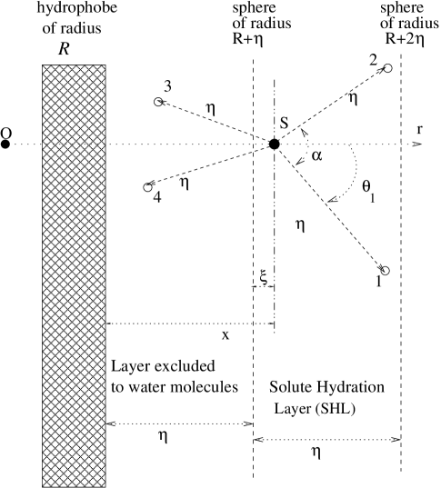
Figure 1:

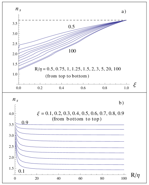
Figure 2:

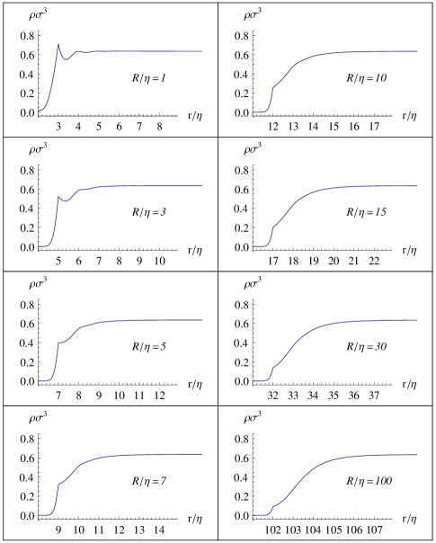
Figure 3:

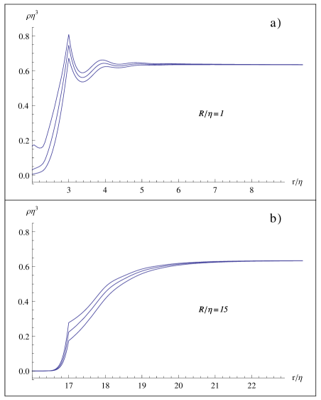
Figure 4:

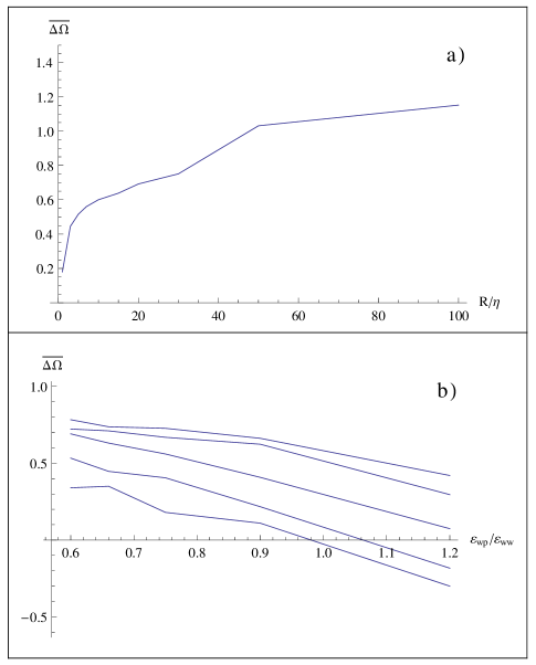
Figure 5:

TOC Graphic