Radial sine-Gordon kinks as sources of fast breathers

Abstract

We consider radial sine-Gordon kinks in two, three and higher dimensions. A full two dimensional simulation showing that azimuthal perturbations remain small allows to reduce the problem to the one dimensional radial sine-Gordon equation. We solve this equation on an interval $[r_{0},r_{1}]$ and absorb all outgoing radiation. Before collision the kink is well described by a simple law derived from the conservation of energy. In two dimensions for $r_{0}\leq 2$, the collision disintegrates the kink into a fast breather while for $r_{0}\geq 4$ we obtain a kink-breather meta-stable state where breathers are shed at each kink ”return”. In three and higher dimensions $d$ a kink-pulson state appears for small $r_{0}$. The three states then exist as shown by a study of the $(d,r_{0})$ parameter space. On the application side, the kink disintegration opens the way for new types of terahertz microwave generators.

PACS : nonlinear dynamics of solitons 05.45.Yv, microwaves 84.40x

I Introduction

The sine-Gordon equation is an important model both for theory and for applications. It corresponds to a classical field with degenerated ground states ($2n\pi$) eilbeck . In one space dimension, it is integrable via the inverse-scattering transform and it has two main classes of solutions, the kink and the breather. The former is particularly interesting because it is a topological defect separating two regions where the solution is 0 and $2\pi$. In higher dimensions one can introduce the radial kink i.e. a kink which only depends on the radius $r$ and this was studied by a number of authors. Among these Christiansen et al Christiansen79 , Lomdahl80 , Christiansen81 have shown that such kinks with initial velocity exhibit the return effect where they ”grow” up to some radius and then shrink back. Note also the remarkable work by Geicke who described solutions of the radial sine-Gordon Geicke82 ; Geicke84 and indicated that radial kinks are destroyed Geicke83 at the origin in two dimensions. This observation was also reported by Bogolubsky and Makhankhov bm76 . This particular phenomenon is not well understood. Geicke Geicke83 reports in particular a difference in the collapse of the kink in two and three dimensions. To analyze these radial solutions one can assume that the radial term is small so that the system is a perturbed one dimensional sine-Gordon equation. One of the analytical tools is a perturbation theory based on inverse scattering, see the formulation by Maslov Maslov85 . When the radius is small, however, this breaks down and only conservation laws can be used so the analysis becomes very difficult. For example see the techniques used by Alfimov and Vazquez Alfimov00 to study the long lived radial breathers, so-called ”pulsons”. Using this combination of analysis and numerics, they showed that these waves decay very slowly and in fact do not exist as suchAlfimov00 .

On the application side, the two dimensional sine-Gordon equation describes the electrodynamics of a Josephson junction between two superconducting films in the absence of external current and dissipation barone . The wave part comes from Maxwell’s equations and the sine nonlinearity from Josephson’s constitutive relation. The variable is the phase difference (or flux) $\psi$ between two superconductors. In this context the kink solution, a ”fluxon” carries a flux quantum which generates micro-wave radiation in the terahertz range when it collides on the boundary of the device. When the lateral geometry of the device is reduced, the fluxon, once created, is ”dragged” towards the narrow edge. This suggested a design of a particle detector Nappi95 and also gave rise to the so-called Eiffel junctions with exponential tapered widthbcs96 ; bcs00 . For these, analysis and a preliminary experimental realization Carapella02 confirmed that no magnetic field is needed to move the kink, current alone suffices. The dynamics was shown to be very regular contrary to the standard rectangular design. Note also the analysis of the resonances by Jaworski j05 .

There is a strong link between this Eiffel design and the radial sine-Gordon model as we will see below. This link, together with the formal studies and the applications inspired us to undertake a numerical study of dynamics of two-dimensional and higher dimensional radial kinks. Since the theory is difficult we relied strongly on numerical studies using a careful procedure. We first solved the two dimensional (2d) sine-Gordon equation for a radial kink and showed that azimuthal perturbations remain small. This justifies the reduction to the radial sine-Gordon equation. We studied this equation numerically for a radial kink initial condition on a finite domain $r_{0}<r<r_{1}$, and absorbed all outgoing radiation. This last point is important because the radiation reflecting from the boundary and coming back into the computational domain can perturb strongly the solution. We varied systematically $r_{0}$ from 10 to 0 to see how the radial term $(d-1)\phi_{r}/r$ in the Laplacian affects the collision. The dimension $d$ is another parameter that we varied and this shows new effects. We consider the radial term as a perturbation of the one dimensional sine-Gordon equation and changing $r_{0}$ we change the magnitude of this perturbation from small to very large.

Before the collision at $r_{0}$, we find that the 2d and 3d radial kinks are well described by a simple equation for the radius obtained from energy conservation. When collision occurs, the kink is always strongly affected when $r_{0}\leq 5$. In two dimensions for $r_{0}\leq 2$ it disintegrates into a fast breather rapidly ejected away from $r_{0}$. For larger $r_{0}$ we observe a semi-stable kink-breather bound state which sheds fast breathers at each ”return”. In all cases the kink decays to 0. Interestingly in three dimensions for $r_{0}=5$ we recover the total destruction of the kink. For $r_{0}\leq 5$ all the kink energy cannot be converted into a single breather because the radial term is too strong to prevent it from escaping. Instead we observe a kink-pulson bound state that ejects small high-frequency (low energy) breathers. For $d\geq 3$ the collision can yield the three states as shown by a study of the $(d,r_{0})$ parameter plane. This scenario explains the differences observed by Geike Geicke83 and other authors for the two and three dimensional kink collision. It also opens an avenue for new microwave devices which transform a fluxon (kink) into a large microwave pulse.
The article is organized as such. In section II we illustrate the collapse of a sine-Gordon kink in two dimensions and show that there are no azimuthal effects. This justifies the reduction to the radial sine-Gordon equation. Section III is the study of its conservation laws. Using these we deduce a simple model for the shrinking. We examine in detail the radial kink collision in two, three and higher dimensions in section IV and characterize the emission of breathers. We conclude in section V and suggest a design for a terahertz radiation source.

II The collapse of a Sine-Gordon kink in a 2d sector

To illustrate the problem that we will consider we present here a 2d numerical study of the dynamics of a radial kink in a sector. The 2d sine-Gordon equation reads

$$\psi_{tt}-{\psi_{\theta\theta}\over r^{2}}-\psi_{rr}-{\psi_{r}\over r}+\sin\psi=0.$$ (1)

As domain we consider the sector $r_{0}<r<r_{1}$, $0<\theta<\theta_{0}$ shown in Fig. 1. The boundary conditions corresponding to no external current are homogeneous Neuman so that $\psi_{\theta}=0$ for $\theta=0,\theta_{0}$ and $\psi_{r}=0$ for $r=r_{0},r_{1}$.

Figure 1: Sketch of the 2d domain for the sine-Gordon equation. The radial kink initial condition is shown as a dotted-dashed line.

We consider the propagation of a sine-Gordon kink inside such a sector. In that case the initial condition is given by eilbeck

$$\phi(r,t=0)=4{\rm atan}(\frac{r-R_{0}}{\sqrt{1-u_{0}^{2}}}),$$ (2)

where $R_{0},u_{0}$ are respectively the initial position and velocity of the kink.

Figure 2: Snapshots of the evolution of a kink for the 2d sine-Gordon equation in a wedge. The kink is started at $R_{0}=12$ in a domain such that $r_{0}=1,r_{1}=20$. The top panel shows the solution for $t=9$ before collision and the bottom panel the solution for $t=25$ after the collision. The $z$ range for the top plot is $[0;2\pi]$ while for the bottom plot it is $[-\pi;\pi]$.

We have computed the evolution of such an initial condition using the comsol finite element software comsol . Fig. 2 shows two different snapshots of the evolution of a kink in a domain such that $r_{0}=1,r_{1}=20$ assuming $R_{0}=10$ and $u_{0}=0$. On the top panel, showing the kink at $t=9$, the kink is accelerated towards the narrow edge. Notice the absence of radiation and the characteristic overshoot. The bottom panel presents the solution after collision $t=25$ and shows that the kink has disappeared and only a flat background $\phi\approx 2\pi$ persists with some oscillations. Despite the violence of the collision all the energy remains in the radial $n=0$ mode and no azimuthal modes are excited. The space discretisation (finite elements) does not preserve the radial symmetry. Nevertheless azimuthal perturbations do not grow. We therefore now look for a reduction of the model to the radial case and justify this approximation.

To reduce the 2d problem it is natural to expand in azimuthal modes using the cosine Fourier series

$$\psi(r,\theta,t)=\sum_{n=0}^{\infty}\phi_{n}(r,t)\chi_{n}(\theta),$$ (3)

where $\chi_{n}(\theta)=\cos(\frac{n\pi\theta}{\theta_{0}})$. Plugging the expression (3) into (1) and projecting onto $\chi_{0}$ we obtain the evolution of $\phi_{0}$

$$-{\phi_{0}}_{tt}+{\phi_{0}}_{rr}+\frac{{\phi_{0}}_{r}}{r}=\frac{1}{\theta_{0}}\int_{0}^{\theta_{0}}\sin(\phi_{0}+\phi_{1}\chi_{1}+\phi_{2}\chi_{2}+\dots)d\theta.$$ (4)

The integrand in the right hand side can be written as

$$\sin(\phi_{0}+\phi_{1}\chi_{1}+\dots)=\sin(\phi_{0})\cos(\phi_{1}\chi_{1}+\phi_{2}\chi_{2}+\dots)$$

$$+\cos(\phi_{0})\sin(\phi_{1}\chi_{1}+\phi_{2}\chi_{2}+\dots).$$

The integral on the right hand side of (4) becomes

$${\sin(\phi_{0})\over\theta_{0}}\int_{0}^{\theta_{0}}d\theta\cos(\phi_{1}\chi_{1}+\phi_{2}\chi_{2}+\dots)$$

$$+{\cos(\phi_{0})\over\theta_{0}}\int_{0}^{\theta_{0}}d\theta\sin(\phi_{1}\chi_{1}+\phi_{2}\chi_{2}+\dots).$$

To estimate these terms we expand the cosine and sine. Then we find that the non zero contribution for the first term will yield terms of the form

$${\phi_{i}^{2}\over 2}\sin(\phi_{0}),$$

and will yield cubic terms for the second integral. This shows that if the $\phi_{i}$ are small, one can assume that

$$\sin(\phi_{0}+\phi_{1}\chi_{1}+\dots)\approx\sin(\phi_{0})+\cos(\phi_{0})(\phi_{1}\chi_{1}+\phi_{2}\chi_{2}+\dots),$$

so that (4) reduces to the radial 1D sine-Gordon equation

$$-{\phi}_{tt}+{\phi}_{rr}+\frac{{\phi}_{r}}{r}=\sin(\phi),$$ (5)

where the $0$’s have been omitted for simplicity. The model (5) can be obtained for any angle $\theta_{0}$ and in particular for the whole two-dimensional sector. It is also linked to the variable width sine-Gordon equation which contains the term $\phi_{x}~{}w^{\prime}(x)/w(x)$ bcs96 . The radial sine-Gordon corresponds to $w(x)=\theta_{0}x$ while the Eiffel junction is for $w(x)=w_{0}e^{-\lambda x}$.

III Numerical procedure

We now detail the numerical procedure because it is the basis of this work. Another reason is that the approximate analysis based on perturbation methods is difficult to validate a priori for small radiuses. We give it meaning by comparing the predictions to the numerical solution. We solve the radial sine-Gordon equation using the method of lines where the space discretisation is done using a finite difference and the time advance is done using an ode solver (DOPRI5 ordinary differential equation solver Hairer ). This method is flexible and one can increase easily the space discretisation. Another time integrator we have used for comparison is the Verlet method lr04 . The number of discretisation points for a typical run is 4000 and the accuracy is checked by computing the hamiltonian H (10). For all cases presented the relative error is smaller than $210^{-5}$. The boundary condition at $r_{0}$ is of the Neuman type so that there is perfect reflection. When $r_{0}=0$ care must be taken because the operator $\phi_{r}/r$ should be regularized because we have an indetermination $0/0$. The way to do this is to invoke the limit

$$\frac{\phi_{r}}{r}=\frac{\phi_{r}(r,t)-0}{r-0}\to_{r\to 0}\phi_{rr}(r=0,t),$$ (6)

so that $\phi_{rr}+\phi_{r}/r|_{r=0}=2\phi_{rr}|_{r=0}$.

At the instant of collision radiation is emitted from the kink. To avoid it re-entering the computational domain we introduce a ”sponge layer” where waves are damped so that the equation becomes

$${\phi}_{tt}-{\phi}_{rr}-(d-1)\frac{{\phi}_{r}}{r}+\sin(\phi)=-\alpha(r){\phi}_{t},$$ (7)

where $\alpha(r)$ increases smoothly from $r_{d}=0.9r_{1}$ to the edge of the domain $r_{1}$ as shown in Fig. 3. This mechanism kills all radiation that travels to the right and exits the computational domain. The amount of energy leaving the computational domain is then computed using the flux relation (12) evaluated at $r_{f}<r_{d}$. This ”sponge layer” is better adapted for our purposes than a perfectly patched layer because it damps all out-going waves not only the ones of speed one.

Figure 3: Sketch of the 1D computational domain.

The equation (5) is not integrable as in the 1d case and there are only a finite number of conservation laws. These are the main analytical tool to study the solution. We consider them in the next section.

IV Conservation laws

The radial sine-Gordon equation in $d$ dimensions

$${\phi}_{tt}-{\phi}_{rr}-(d-1)\frac{{\phi}_{r}}{r}+\sin(\phi)=0,$$ (8)

in a finite domain $[r_{0},r_{1}]$ possesses the following energy conservation law.

$${dH\over dt}=[r^{d-1}\phi_{r}\phi_{t}]_{r_{0}}^{r_{1}},$$ (9)

where the Hamiltonian $H$ is

$$H=\int_{r_{0}}^{r_{1}}r^{d-1}dr[{\phi_{t}^{2}\over 2}+{\phi_{r}^{2}\over 2}+(1-\cos\phi)]\equiv\int_{r_{0}}^{r_{1}}r^{d-1}dr{\cal H}.$$ (10)

To see this multiply (8) by $\phi_{t}$, integrate over the domain and integrate by parts the $\phi_{r}$ term. Assuming a Neuman boundary condition at $r=r_{0}$ we naturally obtain the flux relation for the energy

$${dH\over dt}={r_{1}}^{d-1}\phi_{r}\phi_{t}|_{r_{1}}.$$ (11)

By integrating this relation over time we obtain

$$H(t)=H(0)+\int_{0}^{t}\phi_{r}(r_{1},t^{\prime})\phi_{t}(r_{1},t^{\prime})dt^{\prime}$$ (12)

This enables us to compute how much energy leaves the computational domain at $r=r_{f}$. The energy conservation will be crucial to explain many properties of the solution.

Another conservation law is related to the momentum $\Pi$ of the wave defined as

$$\Pi=\int_{r_{0}}^{r_{1}}r^{d-1}dr\phi_{t}.$$ (13)

From the partial differential equation (8) we get

$${d\Pi\over dt}=[r^{d-1}\phi_{r}]_{r_{0}}^{r_{1}}-\int_{r_{0}}^{r_{1}}r^{d-1}dr\sin\phi,$$ (14)

which shows that even for Neuman boundary conditions at $r=r_{0},r_{1}$ the momentum is not conserved.

For a localized wave such as a kink, the integrands in $H$ and $\Pi$ are highly localized in $r$. In 2d we can get a good approximation of the motion before collision by using the kink solution to the 1D sine-Gordon equation as an ansatz

$$\phi_{k}=4{\rm atan}[\exp({r-R\over\sqrt{(}1-{\dot{R}}^{2})})],$$ (15)

where $R$ is the kink position. We assume that the kink is not too close to the boundary so the integral can be taken from $-\infty$ to $\infty$.

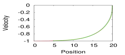
Figure 4: Top panel: 2d radial kink velocity for $r_{0}=0,5$ as a function of the position $R$. The velocity obtained from the numerical solution is given by the points and the analytical estimate (17) is given by the dashed line. Bottom panel: 3d radial kink velocity for $r_{0}=0,5$ as a function of the position $R$. The velocity obtained from the numerical solution is given with the points and the analytical estimate (21) is given by the dashed line.

To calculate it we change the integration variable so that $r-R=r^{\prime}$ and write

$$H=R\int_{-\infty}^{+\infty}{\cal H}dr^{\prime}+\int_{-\infty}^{+\infty}r^{\prime}dr^{\prime}{\cal H}.$$

The second integral is then 0 because of parity. This gives

$$H\approx 8{R\over\sqrt{1-({\dot{R}})^{2}}}.$$ (16)

At $t=0$ we start the kink at $R=R_{0}$ with $u_{0}$ initial velocity so that $H=8R_{0}$. From that one can compute the velocity $u={\dot{R}}$ as a function of $R$

$$u=\pm\sqrt{1-({R\over R_{0}})^{2}(1-u_{0}^{2})}.$$ (17)

Fig. 4 shows the velocity $u$ vs the position $R$ of a 2d radial kink (top panel) and the 3d radial kink (bottom panel) obtained from the numerical solution as it propagates towards $r_{0}$ for $r_{0}=0,1,5$ and 10. The velocity is estimated by assuming the kink functional dependance (15). One then estimates

$${\rm Max}(\phi_{t})={2u\over{1-u^{2}}},$$

and deduces the velocity $u$. On the same plot we report the estimate (17). The picture shows that the agreement is very good even when the kink is close to $r_{0}$. Assuming the wave keeps it’s kink profile, its position $R$ follows the differential equation obtained from (16)

$${\ddot{R}}+{R\over R_{0}^{2}}=0.$$ (18)

whose solution is

$$R(t)=R_{0}\cos{t\over R_{0}^{2}}.$$ (19)

As expected bcs96 the kink travels towards the ”narrow” end and accelerates.

Using similar arguments we can reduce the Hamiltonian for the 3d kink to

$$H=R^{2}\int_{-\infty}^{+\infty}{\cal H}dr^{\prime}+\int_{-\infty}^{+\infty}r^{\prime 2}dr^{\prime}{\cal H}.$$

The first term gives

$$H\approx 8{R^{2}\over\sqrt{1-({\dot{R}})^{2}}}.$$ (20)

The second term is a small correction of the order of the cube of the ”width” of the kink. It is much smaller than the leading term (20). We then obtain the evolution of the 3d radial kink as

$$u=\pm\sqrt{1-({R\over R_{0}})^{4}(1-u_{0}^{2})}.$$ (21)

The comparison of (21) with the numerical solution is also very good as shown in the bottom panel of Fig. 4. The differential equation for $R$ is

$${\ddot{R}}+{2R^{3}\over R_{0}^{4}}=0,$$ (22)

which implies a decay of $R$ but does not have a simple solution.

V Radial kink collision in 2d and 3d

To understand the collision of a kink with the boundary at $r=r_{0}$ we have conducted extensive numerical studies varying systematically $r_{0}$. The main result for both 2d, 3d and larger d is that the kink does not survive collision in a proper way when $r_{0}$ is small. It decays after a few collisions and at each collision it emits part of its energy in the form of fast breathers that escape the radial potential. This is true for all initial conditions $R_{0}>10$. This is interesting since it is a way to destroy a topological defect. The specifics vary from the 2d case to the 3d case so we will consider them separately.

Figure 5: 2d radial kink collision for $r_{0}=0$. Plot of $\phi(x,t)$ as a function of $x$ for $t=11,~{}16,~{}21,~{}26,~{}31$ and $36$ (top panel) and $t=41,61$ (bottom panel). The kink is started at $R_{0}=20$. The parameters are $r_{0}=0,r_{1}=40$.

V.1 collision in 2d

Figure 6: 2d radial kink collision. Time evolution of the energy exiting the domain at $r_{f}=30$, for $r_{0}=0,5$ and 10. The kink is started at the same position $R_{0}=20$ so the initial energy $H_{0}\approx 160$ is the same for the three cases.

Fig. 5 shows snapshots of $\phi(x,t)$ as a function of $x$ for different times before and after the collision at $r_{0}=0$. The top panel shows the times $t=11,\dots 36$ corresponding to the kink being accelerated towards $r_{0}=0$. Notice the large overshoot for $t=36$. The right panel of Fig. 5 shows the two instants $t=41$ and $t=61$ showing that very little is left of the initial kink. There is just a small disturbance around $2\pi$ traveling towards large $r$. In fact all the kink energy from (16) $H\approx 20\times 8=160$ leaves the computational domain as shown by the energy flux (12) measured at $r=30$ shown in Fig. 6.

The wave present in the domain after the collision is a fast breather. Recall that a sine-Gordon breather is given by

$$\phi_{b}=4{\rm atan}\left[{\sqrt{1-\omega^{2}}\cos(\omega\gamma(t-ur-t_{0}))\over\omega\cosh(\sqrt{1-\omega^{2}}\gamma(r-R_{0}-ut))}\right],$$ (23)

where $\gamma$ is the usual Lorentz factor

$$\gamma={1\over\sqrt{1-u^{2}}}.$$

The energy of the breather on the infinite line is given by scott

$$H=16\gamma\sqrt{1-\omega^{2}},$$

so that using the same argument as for the kink we get for the radial case

$$H_{b}=16R\gamma\sqrt{1-\omega^{2}},$$ (24)

where $R$ is the center of mass of the breather. To identify this fast breather in the numerical solution we have plotted the position of its center of mass as a function of time on the top panel of Fig. 7. The velocity estimated by the fit (dashed line) is $u\approx 0.89$. On the middle and bottom panels we have plotted the analytical expression of the breather (23) added to the $2\pi$ background together with the numerical solution for $t=41$ and $t=46$. The parameters used for the fitting are

$$\omega=0.82,~{}~{}t_{0}=-3,~{}~{}x_{0}=9.2$$

As can be seen the fit is very good, the error in the energy between the fit and the numerical solution is 10 %. Such a breather can ”escape” the radial trap because its high frequency averages out the radial force. Also note that the radial wave equation does not support any traveling wave like in the 1D case, so any emitted radiation has to be in the form of a wave packet. It is interesting to find breather solutions as a product of the disintegration of a kink. In the 1d case for which the sine-Gordon equation is integrable, the breather and kink-antikink pairs are separated. Here, with the radial term a connection has been opened between the two states. This is similar to the numerical experiments of dsv08 where kink-antikink pairs are created out of a train of small breathers in the $\phi^{4}$ model which is a perturbation of the sine-Gordon equation.

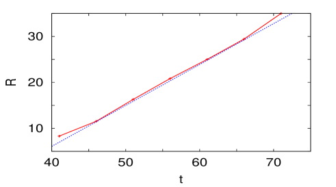
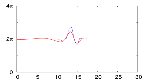
Figure 7: Characterization of the wave after 2d radial kink collision. The top plot shows the center of mass of the wave as a function of time. The middle and bottom plots show the numerical solution together with the breather fit (23) for $t=41$ and $t=46$ respectively.

For a larger value of the boundary $r_{0}=5$, the kink is reflected and looks roughly like an antikink. The snapshots are shown in Fig. 8. Notice the return occurring for $t\approx 41$. There is however about 20 % of energy (about 21) lost after the collision, as shown in the flux plot Fig. 6. The approximate antikink that is formed has an energy which is about $16\times 8=128$ so that it ”stops” at $R\approx 16$ as shown in the bottom panel of Fig. 8. Again a breather is emitted, it is bound to the antikink up to $t=41$ after which it detaches and propagates to the right.

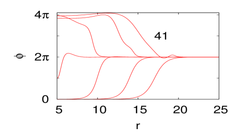
Figure 8: 2d radial kink collision for $r_{0}=5$. The top panel shows plots of $\phi(x,t)$ as a function of $x$ for $t=11,~{}16,~{}21,~{}26,~{}31,~{}36$ and $41$. The bottom panel shows snapshots of $\phi(x,t)$ for $t=41$ and $61$. The kink is started at $R_{0}=20$. The parameters are $r_{0}=5,r_{1}=40$.

To characterize this breather we ran the simulation over a much larger space interval $r_{1}=100$. The parameters of the breather can be calculated as follows using the energy loss

$$H(t=0)-H(t=81)\approx 21=x_{0}16{\sqrt{1-\omega^{2}}\over\sqrt{1-u^{2}}}$$

with $x_{0}=30$ corresponding to an instant of observation $t=80$. This gives the following parameters

$$u=0.7,~{}~{}\omega=0.9995$$

which are consistent with the energy loss (21) and the duration of the breather passing through the boundary

$$\delta t={\rm width}/{\rm speed}={\sqrt{1-\omega^{2}}\over\gamma u}\approx 32.$$

After the emission of this breather, the kink continues to oscillate and decays slowly emitting waves at each collision with $r=r_{0}$. For larger $r_{0}$ as shown in Fig. 6 for $r_{0}=10$ the kink decays much slower. For $t=100$ its energy has diminished by about 10 %. At every collision some energy is expelled. For such value $r_{0}$ the radial term $\phi_{r}/r$ is small and we are close to the one dimensional situation.

To shed another light on the problem it is useful to examine the different conservation laws before and after collision. We analyzed the difference between $r_{0}=0$ and $r_{0}=5$, by computing the momentum $\Pi$, the right hand side $S$ in the flux of the momentum (14) and the front position $R$. The latter is defined as the maximum of $\phi_{x}$. The time evolution of the three quantities $\Pi,S$ and $R$ are shown in Fig. 9. The top panel corresponds to $r_{0}=0$ and the bottom panel to $r_{0}=5$.

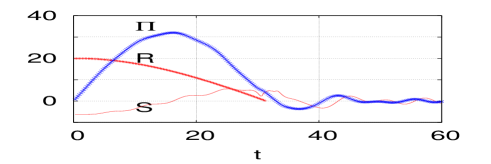
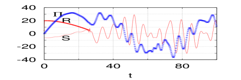
Figure 9: 2d radial kink collision. Time evolution of the rescaled momentum $\Pi/2$, the kink position $R$, and the source term $S$ of the momentum equation for $r_{0}=0$ (top panel) and $r_{0}=5$ (bottom panel).

For $r_{0}=0$ the momentum $\Pi$ goes through 0 for $R=0$ (collision instant). There $S>0$ so that $\Pi$ will keep decreasing and oscillate around zero, indicating that the soliton is destroyed. For $r_{0}=5$ shown in the bottom panel, $\Pi>0$ at collision and $S>0$ so that $\Pi$ remains positive for $t\geq 20$. After that instant $S$ starts to oscillate with a period about 6. $S$ is largely positive so that $\Pi<0$ on average. We then reach $\Pi=0$ so that the kink stops at $t\approx 41$ for which $R=15$. This is the return effect.

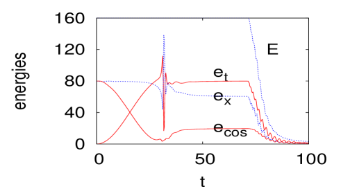
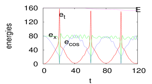
Figure 10: 2d radial kink collision: Time evolution of the energy components $e_{t}=\int_{r_{0}}^{r_{1}}0.5x\phi_{t}^{2}dx$, $e_{x}=\int_{r_{0}}^{r_{1}}0.5x\phi_{x}^{2}dx$ and $e_{p}=\int_{r_{0}}^{r_{1}}(1-cos\phi)xdx$ for a kink. On the top panel $r_{0}=0$ while on the bottom panel panel $r_{0}=10$. The kink is started at the same position $R_{0}=20$.

The total energy is conserved but gets distributed differently between the different components, the kinetic term $e_{t}=\int_{r_{0}}^{r_{1}}0.5\phi_{t}^{2}x~{}dx$, the gradient term $e_{x}=\int_{r_{0}}^{r_{1}}0.5x\phi_{x}^{2}dx$ and the potential term $e_{p}=\int_{r_{0}}^{r_{1}}(1-cos\phi)x~{}dx$. Initially the kink has 0 velocity so that $e_{t}=0$, all the energy is concentrated in $e_{x}$ and $e_{p}$. For $r_{0}=0$ on the top panel of Fig. 10, the kinetic term $e_{t}$ increases from 0 to its maximum at the collision and then remains about constant. The potential term $e_{p}$ decreases from its maximum value at $t=0$ and stabilizes around half its value. The behavior is different for $r_{0}=10$ shown on the bottom panel of Fig. 10, for which the collision is almost elastic. There at the instant of collision, the kinetic energy reaches its maximum, the total energy and the potential energy and gradient energies are almost zero. After collision both recover their initial values.

V.2 Collision in 3d and higher d

We now consider the collision of a kink in 3d and higher d to see if there are particular situations. The general result that radiation is emitted as fast breathers out of the computational domain still holds. As an example consider the flux of the energy shown for the 3d case in Fig. 11 for $r_{0}=0,~{}5$ and $10$.

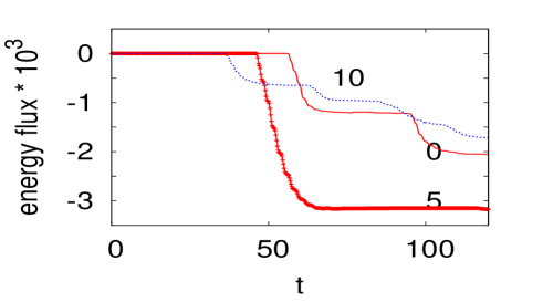
Figure 11: Time evolution of the energy flux for three different values $r_{0}=0,5$ and 10. The kink is started at the same position $R_{0}=20$ so the initial energy $H_{0}\approx 3200$ is the same for the three cases.

Interestingly the case $r_{0}=5$ is similar to the 2d case for $r_{0}=0$. The kink is entirely transformed into a fast breather that exits the computational domain. This is shown in the series of snapshots in Fig. 12. The fast breather is clearly seen traveling to the right at time $t=31$. For $r_{0}=0$ there is a bound state kink/breather so that the kink ”sheds” a breather at every collision with the boundary and decays. Fig. 13 shows the successive snapshots of the solution in this case. The solution for $t=31$ is clearly a combination of a kink and a breather.

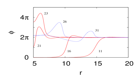
Figure 12: 3d radial kink collision for $r_{0}=5$: plot of $\phi(x,t)$ as a function of $x$ for $t=11,~{}16,~{}21,~{}23,~{}26$ and 31. The snapshots after the collision are indicated in dashed line (blue online). The kink is started at $R_{0}=20$. The parameters are $r_{0}=5,r_{1}=40$.

For such a large value of $d$ and such a small $r_{0}$ the radial term $(d-1)\phi_{r}/r$ is very strong and prevents a low frequency breather from escaping. Only breathers of frequency $\omega\approx 1$ can escape and these have fairly low energy. Such a breather will be ”shed” from the kink as it reaches its return point, around $R=5$. The energy and momentum behave in a very similar way as in the 2d case so we do not present them.

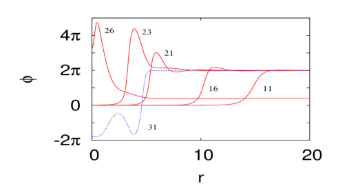
Figure 13: 3d radial kink collision for $r_{0}=0$: plot of $\phi(x,t)$ as a function of $x$ for $t=11,~{}16,~{}21,~{}23,~{}26$ and 31. The field for the snapshot $t=23$ has been divided by 5 to fit in the plot. The kink is started at $R_{0}=20$. The parameters are $r_{0}=0,r_{1}=40$.

To confirm these findings we conducted two simulations with $d=5$, for $r_{0}=0$ and $5$ and $r_{1}=40$. The flux of energy exiting the domain is shown in Fig. 14. It shows two breathers being emitted respectively at $t=55$ and $t=100$ for $r_{0}=0$.

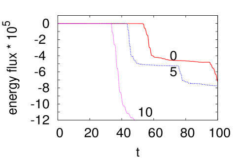
Figure 14: Energy exiting the computational domain $[r_{0}:100]$ for $d=5$ and $r_{0}=0$ in continuous line (red online) and $r_{0}=5$ in dashed line (blue online). The total energy is 1.295743 $\times 10^{6}$.

The $(d,r_{0})$ parameter plane is shown in Fig. 15. It shows the coexistence of the three states, the fast breather (B), the kink-breather metastable (KB) and the kink-pulson metastable state (KP) Interestingly the last one cannot be seen for $d=2$.

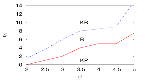
Figure 15: Parameter plane $(d,r_{0})$ showing the different possible outcomes for a kink collision, a fast breather (B), a kink-pulson metastable state (KP) and a kink-breather metastable state (KB).

VI Conclusion

Motivated by theory and applications, we studied radial sine-Gordon kinks in two and higher dimensions. A full two dimensional simulation showed that azimuthal perturbations remain small. We therefore reduced the problem to the one dimensional radial sine-Gordon equation which we solve on an interval $[r_{0},r_{1}]$. Before collision the kink is well described by a simple law derived from the conservation of energy. In two dimensions the collision of the kink with the boundary $r_{0}$ will result in a fast breather for small $r_{0}$ and in a kink-breather metastable state for larger $r_{0}$. In the latter, the kink sheds at each ”return” a large part of its energy into bursts which are breather solutions. We have characterized these waves in terms of their energy, frequency and velocity. In three and higher dimensions and small $r_{0}$ we observe a kink pulson bound state. The three states exist in the $(d,r_{0})$ parameter space. This study shows that radial perturbation opens a channel between the kink solutions and the breather solutions. This is particularly interesting because in one dimension these are completely separated. This additional term provides therefore a mechanism to ”destroy” these topological defects and extract the energy they contain.

In view of applications to 2d Josephson junctions this could be very useful to generate Terahertz radiation. At this time output from these devices is low. Here for small $r_{0}$ all the kink energy is converted into radiation. This suggests the design of a new device based on window Josephson junctions. A sketch of the device is shown in Fig. 16. The top panel shows a top view of the junction together with the radio-frequency detector D. Notice the current input similar as in Carapella02 with its passive region separating the electrodes. The bottom panel shows a side view of the system with the oxide layer O separating the two superconducting films. As the current $I$ is increased a train of fluxons is formed. These reflect into the narrow end $r=r_{0}$ and fast breathers are formed which consist in bursts of microwave. Since all the kink energy is converted into microwaves, we expect this system to generate much more radiation than a standard flux-flow.

Figure 16: Sketch of a microwave generator based on a radial Josephson window junction.

VII Acknowledgements

The authors thank Egor Alfimov, Peter Christiansen and Yuri Gaididei for very helpful discussions. J. G. C. thanks the Institute of Mathematical Modeling and the Department of Mathematics at the Technical University of Denmark for their hospitality during several visits. The authors acknowledge the Centre de Ressources Informatiques de Haute Normandie where most of the calculations were done. J. G. C. is on leave from Laboratoire de Mathématiques, INSA de Rouen, France.

References

- (1) R. K. Dodd , J. C. Eilbeck , J. D. Gibbon and H. C. Morris, Solitons and Nonlinear Wave Equations, Academic Press, (1984).
- (2) P.L. Christiansen and O.H. Olsen, Physica Scr. 20, 531-538 (1979); Phys. Letts. A, 68, 185-188, (1978).
- (3) P.S. Lomdahl, O.H. Olsen and P.L. Christiansen, Phys. Letts. A, 78(2), 125-128, (1980).
- (4) P.L. Christiansen and P.S. Lomdahl, Physica 2D, 482-494, (1981).
- (5) J. Geicke, Physica 4D, 197-206, (1982).
- (6) J. Geicke, Physica Scripta , 29, 431-434, (1984).
- (7) J. Geicke, Physics Letters 98A, 147-150, (1983).
- (8) I. L. Bogolubsky and V. G. Makhankov, Zh. Eksp. Teor. Fiz. Pis’ma Red. ,24, 15, (1976). (J.E.T.P. Lett. 24, 12, (1976).)
- (9) E. M. Maslov, Phisica 15D, 433-443, (1985).
- (10) G.L. Alfimov, W.A.B. Evans and L. Vàzquez, Nonlinearity, 13, 1657-1680, (2000).
- (11) A. Barone and G.-F. Paterno, Physics and Applications of the Josephson Effect John Wiley and sons INC, N. Y. (1982).
- (12) S. Pagano, C. Nappi, R. Cristiano, E. Esposito, L. Frunzio, L. Parlato, G. Peluso, G. Pepe and U. Scott Di Uccio, in Nonlinear superconducting devices and high Tc materials, World scientific, Singapore, (1995).
- (13) A. Benabdallah, J. G. Caputo and A.C. Scott, Phys. Rev. B., vol 54, 16139-16147, (1996).
- (14) A. Benabdallah, J. G. Caputo et A. C. Scott, J. Appl. Physics, vol. 88, nb. 6, 3527-3540, (2000)
- (15) G. Carapella, N. Martucciello and G. Costabile Phys. Rev. B 66, 134531 (1-7), (2002).
- (16) M. Jaworski, Phys. Rev. B 71, 214515, ̵͑(2005͒).
-
(17)
Comsol Multiphysics modeling and simulation software
http://www.comsol.com/ - (18) E. Hairer, S. P. Norsett and G. Wanner. Solving ordinary differential equations I, Springer-Verlag, (1987).
- (19) B. Leimkhuler and S. Reich, Simulating hamiltonian dynamics, Cambridge University Press, (2004).
- (20) A. C. Scott, Nonlinear Science, Oxford University Press, (1999).
- (21) S. Dutta, D. A. Steer and T. Vachaspati, Phys. Rev. Lett. 101, 121601 (2008)