Modeling temporal networks using random itineraries
Abstract
We propose a procedure to generate dynamical networks with bursty, possibly repetitive and correlated temporal behaviors. Regarding any weighted directed graph as being composed of the accumulation of paths between its nodes, our construction uses random walks of variable length to produce time-extended structures with adjustable features. The procedure is first described in a general framework. It is then illustrated in a case study inspired by a transportation system for which the resulting synthetic network is shown to accurately mimic the empirical phenomenology.
pacs:
89.75.-k, 89.75.Hc, 02.50.Ey , 05.40.Fb , 89.75.FbMany systems in nature or related to human activities are conveniently represented as networks of interacting units that can exchange material or information. This approach, combined with techniques from graph theory, statistical physics and data analysis, has led to countless interesting studies and insights in numerous fields science ; Dorogovtsev:2003 ; Newman:2003 ; Pastor:2004 ; Caldarelli:2007 ; Barrat:2008 .
Until recently, network structures were often regarded as being stationary, both for simplicity and because of scarceness of datasets on the time variability of connectivity patterns. Thanks to advanced acquisition technologies and large scale production of time-resolved data, temporal information has become more accessible in numerous contexts, from communication networks Eckmann:2004 ; Onnela:2007 ; Makse:2009 ; Amaral:2009 ; Karsai:2012 to proximity patterns Cattuto:2010 ; Salathe:2010 and infrastructure networks Gautreau:2009 ; Bajardi:2011 . This has led to the recent surge of activity in the field of “temporal networks” review_holme . Data analysis revealed the coexistence of statistically stationary properties and local variations, interaction burstiness Eckmann:2004 ; Holme:2005 ; Onnela:2007 ; Makse:2009 ; Amaral:2009 ; Gautreau:2009 ; Cattuto:2010 ; Salathe:2010 ; Bajardi:2011 ; Karsai:2012 ; humdyn-barabasi ; humdyn-vazquez ; Barabasi:2010 ; review_holme and the occurrence of non-local repetitive patterns Bajardi:2011 ; kovanen:2011 . These structural properties affect the dynamical processes taking place on networks Vazquez:2007 ; Iribarren:2009 ; Miritello:2011 ; Isella:2011 ; Karsai:2011 ; Bajardi:2012 ; Holme:2013 ; Hoffmann:2012 ; Perra:2012PRL ; Ribeiro:2012 . Therefore, they have to be accounted for in modeling approaches.
Despite the proliferation of temporally resolved datasets, strong limitations perdure. Indeed, data are often only accessible in restricted forms, such as single samples of limited sizes and statistical relevance. Comparison of connection patterns at different times is not always possible. Some datasets consist only of aggregated information and do not provide access to the temporal course of events. In such circumstances, it is necessary to be able to generate synthetic time-extended structures whose aggregation would reproduce the data at hand. This would enable one to go beyond the approximation of static networks and to incorporate dynamical components in network structures.
Several models of temporal networks have been proposed in the literature GB08 ; Gautreau:2009 ; Latora:2010 ; Stehle:2010 ; Perra:2012 ; Starnini:2013 . Their dynamics mostly consist of link updates and show that a global complex space-time organization can emerge as the result of simple pairwise cooperation or competition rules between individual units. Dataset randomization is also employed to create null models against which the temporal pattern complexity of empirical data can be evaluated review_holme ; Karsai:2011 .
The modeling approach developed in this Letter is to some extent more direct and pragmatic. It is intended to provide a versatile procedure for the construction of time-dependent networks with adjustable characteristics, that mimic bursty and possible repetitive behaviors, as well as extended temporal correlations, as they are observed in real world systems. The goal is to obtain realistic temporal structures independently of any access to datasets or assumptions about basic interaction mechanisms.
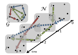
The proposed procedure originates from the observation that in many graphs representing systems such as transportation, trade or communication networks, connection patterns are the result of activity spreading along noisy itineraries within a complex structure. The weighted directed graph used to represent this activity is then given by the accumulation of such itinerary traces. Our construction proceeds in the opposite manner. Starting from a given weighted directed graph , it assumes that this graph is the superposition of random walks in a given time window , and seeks to “unfold” these walks, as schematically illustrated in Fig. 1.
Below, we first describe the construction in a general setting. We then apply it to a case study inspired by a transportation system, and use this real-world system to benchmark the synthetic network. Finally, we put forward a characterization of the topological and temporal correlations that takes into account the heterogeneity of the activity in the network.
Temporal network construction.
The construction takes as input a graph and a time window . Here, is a set of nodes and is a set of weighted directed edges, either obtained from data or built with prescribed properties such as in- and out-degree distributions and/or distributions of link weights (for definitions of degree, weight and strength, see e.g. Barrat:2008 ). The temporal network is built as follows.
(i) First, the following random walk characteristics are chosen: distributions of starting times in , of starting locations in , of walk lengths, and of residence times at each node.
(ii) Then, the random walks are generated independently, one after another, using the characteristics specified above. Each walk defines an itinerary that consists of a list of events with (Fig. 1). At each step, the node is uniformly chosen among the out-neighbors of , and the residence time is drawn from the residence time distribution associated with . Any walk reaching a node with no out-link terminates there, even if it has not yet reached its prescribed length.
(iii) As the construction proceeds, the graph is continuously altered as follows: if a walk passes through the link , the weight is decreased by 1; whenever reaches , the edge is discarded from the graph and cannot be used anymore.
(iv) Walks are generated until all edges have been discarded from . Then, the process terminates.
The temporal network is defined as the union of all the constructed itineraries. By construction, the set of weighted directed edges resulting from the collection of all events in coincides with the original set . Itineraries are interpreted differently depending upon context. For instance, in transportation systems, the event is regarded as a material displacement from to at time . In communication networks, events correspond to transmission of information.
Note also that the construction can be used to model routine/seasonal processes occurring in consecutive time windows, using a “noisy deterministic” rule: for each , a tunable fraction of walks is redrawn in , while the remaining itineraries are repeated identically from to .
We claim that, under suitable choices of input parameters, the network can mimic real-world features, in particular bursty temporal patterns and extended correlations. To support these assertions, we benchmark the synthesized network in a case study inspired by a cattle trade system analysis Bajardi:2011 ; note this example is aimed to illustrate the construction algorithm, rather than to accurately fit specific datasets.
Case study.
In this application, we consider nodes representing farms. The graph is constructed using a variant of the uncorrelated configuration model Catanzaro:2005 . Following statistics reported in Bajardi:2011 , we use as in- and out-degree distributions the power-law (with cut-off at to avoid degree correlations Catanzaro:2005 ). Weights are also power-law distributed according to . Interpreting events in as material displacements, we impose flux conservation at every node so that in- and out-strengths balance, i.e. holds for almost all (in practice, more than of .
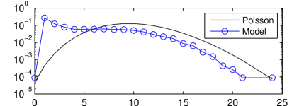
walk length
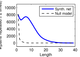
We consider a temporal window of length units (“days”), with periodic boundary conditions, to generate from . To this aim, we use random walks with uniformly distributed starting times and locations. We assign each node a residence time , drawn from for ; a walk visiting node stays for time , plus an additional random delay drawn from a Poisson distribution with mean . (The power-law is inspired by Bajardi:2011 ; similar results are obtained for an exponential .) Walk lengths are generated using a Poisson distribution with average . Notice that since the number of graph edges decreases as the construction proceeds, long walks can seldom be achieved when few edges remain and the realized distribution accordingly exhibits an excess of short paths, see Fig. 2.
Three main types of analysis have been proposed in order to study structural and temporal properties of a time-resolved transportation network Gautreau:2009 ; Bajardi:2011 ; kovanen:2011 : (i) statistics of aggregated networks on various time scales, (ii) distributions of activity and inactivity periods and (iii) repetition of connection patterns such as temporal paths. Here, we show that when applied to the synthetic network , these diagnostics proffer characteristics very similar to those in empirical data.
|
|
|
|---|---|---|
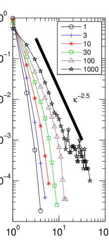
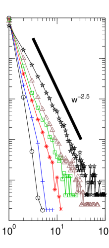
| in-degree | weight | strength |
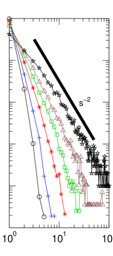
Real world data exhibit robust heterogeneous behaviors at all temporal scales, as asserted by power-law distributions of in-degrees, strengths and link weights Gautreau:2009 ; Cattuto:2010 ; Bajardi:2011 . These distributions remain almost stationary when integrated over distinct windows of equal length. As shown in Fig. 3, the same properties are observed in . These plots also validate the construction algorithm: statistics aggregated over the whole reveal power-law distributions with slopes in close agreement with the corresponding ones in .
|
|
| (a) Node activity time distrib. | (b) Node inactivity time distrib. |
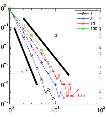
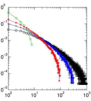
Robust heterogeneous features in transportation networks have also been observed in activity and inactivity period statistics, i.e. in the distributions of the periods during which a node (or a link) is continuously active or inactive. Such observables typically exhibit broad distributions Gautreau:2009 . Fig. 4 reports these distributions for nodes, obtained from using various aggregation scales , from the most detailed (“daily”, ) resolution to coarser timescales mimicking weekly or monthly aggregations (similar results are obtained for links). Activity distributions reveal power-law behaviors in quantitative agreement with empirical data Bajardi:2011 , with decay exponents in the same range of values (increasing from to as the aggregation interval increases). Moreover, distributions of inactivity periods are broader, more concave, and extend across all timescales, as in Bajardi:2011 .
|
|
In addition to burstiness, the activity in shows positive temporal correlations, as can be anticipated from the nature of the construction. In particular, global activity correlations can be appreciated by using
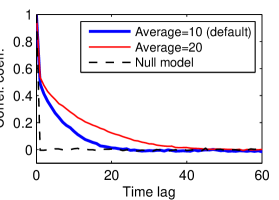
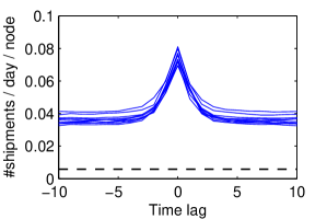
where denotes the total number of events on day and means time averaging over . As Fig. 5 (left) shows, is positive for all in an extended interval, whereas its analog in a null model obtained by reshuffling all links is 0 for any . Note that such a null model is equivalent to a temporal network construction in which we impose all the random walks to have length .
Beside global correlations, local structures can be highlighted by exhibiting chronological link sequences that occur more often than by chance Bajardi:2011 ; kovanen:2011 . A typical example is given by -tolerant temporal paths, i.e. paths composed of consecutive active links within days of each other. The number of such paths is much larger in empirical temporal networks than in reshuffled data Bajardi:2011 . (Note that only the case was considered in Bajardi:2011 .) Fig. 5 (right), which shows the number of -tolerant temporal paths that occur at least twice in , possesses similar features, providing further evidence of the presence of strong correlations in the synthetic network.
Detailed activity correlations
The nature of the temporal network construction, which relies on random walks, suggests that non-trivial local activity correlations should also simultaneously emerge at both topological and temporal levels. Indeed, if a node is active at a certain time, then an elevation of activity should be detected in its topological and temporal neighborhood. (By contrast, such correlations are nonexistent in a model where all links have been reshuffled.) Here, we provide quantitative estimates of these correlations.
In heterogeneous networks such as the current synthetic , local activity patterns are extremely diverse and are hardly captured by global averages such as . Therefore, prior to averaging, we first need to divide the nodes of into categories according to their total activity (defined as the total number of events in , starting from the considered node). The activity at a node in ranges from to over , with average . Accordingly, we define a node as “busy” if its integrated activity exceeds a given threshold, say e.g. (results are qualitatively insensitive to this choice). Furthermore, non-busy nodes are categorized into level sets of the distance to the set of busy nodes , where is measured following the edges in . Altogether, the categories , account for more than of .
For each node category , the correlations between the activity in nodes of at time and in their neighborhood at time are then measured by
where is the average activity per node in a subset of nodes at time ( is the number of events starting from at time ), is the ball of center and radius , and the average is taken over all and such that .
|
|
|
|
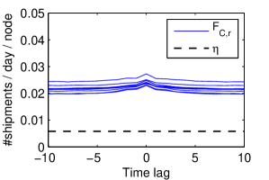
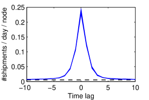
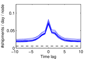
Fig. 6 displays “activity spike curves” vs. for two categories, and , and . In a null model where all links are reshuffled (equivalent to a model built with random walks of length ), each such curve would be perfectly flat except at , where it would take a larger value. In contrast, each curve has a distinctive shape here that is almost insensitive to the network realization. Hence, for each category, these curves provide a characterization of activity correlation patterns in a topological and temporal neighborhood.
The peaked shape of illustrates how the occurrence of activity in the center of a ball is accompanied by an elevated activity in the ball for a number of days before and after. The peaks are substantially sharper for smaller balls (of radius 1), and are instead barely detectable when averaging in the ball of radius 2 around . At large values of , approaches a well-defined baseline level of activity. For , this baseline is higher around busy nodes than around , pointing to a higher level of mean activity in the neighborhood of , as it can be anticipated.
Concluding remarks.
In this Letter, a simple framework for the construction of temporal networks displaying bursty, repetitive and correlated behaviors has been presented, based on random walks on a predefined aggregated graph. The construction is sufficiently versatile to adapt to a wide range of situations, by appropriate tuning of input parameters. In particular, it would be interesting to apply it to initial graphs with community structure. As random walks tend to be trapped inside communities, the construction is expected to naturally give rise to the emergence of temporal communities. Another possible extension would be to use, instead of random walks as building blocks, spreading trees of propagation processes on networks.
Our procedure enables one to obtain plausible and realistic instances of temporal networks when only the aggregated structure is known. Hence, it can be employed to compensate for the lack of time-resolved data or to provide alternative scenarios when access to empirical information is limited. Moreover, that the synthetic network has tunable properties is essential to assessing the influence of time-dependent features on the dynamical processes on networks, especially when only aggregated information is available. Finally, structural flexibility also makes it possible to test the relevance of various definitions of centrality measures for nodes and links in temporal networks.
Acknowledgments. AB and BF are partly supported by FET project MULTIPLEX 317532 and by CNRS PEPS Physique Théorique et ses Interfaces. LSY is supported in part by NSF grant DMS-1101594, and KL by NSF grant DMS-0907927.
References
- (1) Special issue of Science on Complex networks and systems, Science 325, 357 (2009).
- (2) S.N. Dorogovtsev, J.F.F. Mendes, Evolution of networks: From biological nets to the Internet and WWW, Oxford University Press, Oxford 2003.
- (3) M.E.J. Newman, The structure and function of complex networks, SIAM Review 45 (2003) 167-256.
- (4) R. Pastor-Satorras, A. Vespignani, Evolution and structure of the Internet: A statistical physics approach, Cambridge University Press, Cambridge, 2004.
- (5) G. Caldarelli, Scale-Free Networks, Oxford University Press, Oxford, 2007.
- (6) A. Barrat, M. Barthélemy, A. Vespignani, Dynamical processes on complex networks, Cambridge University Press, Cambridge, 2008.
- (7) J.-P. Eckmann, E. Moses, D. Sergi, Proc. Natl. Acad. Sci. USA 101 14333 (2004).
- (8) J.-P. Onnela, J. Saramäki, J. Hyvönen, G. Szabó, D. Lazer, K. Kaski, J. Kertész, A.-L. Barabàsi, Proc. Natl. Acad. Sci. USA 104, 7332 (2007).
- (9) D. Rybski, S.V. Buldyrev, S. Havlin, F. Liljeros, H.A. Makse, Proc. Natl. Acad. Sci. USA 106 (2009) 12640-12645.
- (10) R.D. Malmgren, D.B. Stouffer, A.S.L.O. Campanharo, L.A. Nunes Amaral, Science 325 (2009) 1696-1700.
- (11) M. Karsai, K. Kaski, A.-L. Barabási, J. Kertész, Sci. Rep. 2, 397 (2012).
- (12) C. Cattuto, W. Van den Broeck, A. Barrat, V. Colizza, J.-F. Pinton, A. Vespignani, PLoS ONE 5(7) (2010) e11596.
- (13) M. Salathé, M. Kazandjieva, J.W. Lee, P. Levis, M.W. Feldman, J.H. Jones, Proc. Natl. Acad. Sci. (USA) 107, 22020 (2010).
- (14) A. Gautreau, A. Barrat, M. Barthélemy, Proc. Natl. Acad. Sci. USA 106 8847 (2009).
- (15) P. Bajardi, A. Barrat, F. Natale, L. Savini, V. Colizza, PLoS ONE 6(5):e19869 (2011).
- (16) P. Holme, J. Saramäki, Phys. Rep. 519, 97 (2012).
- (17) P. Holme, Phys. Rev. E 71, 046119 (2005).
- (18) A.L. Barabàsi, Nature 435, 207 (2005).
- (19) A. Vàzquez, J. G. Oliveira, Z. Dezsö, K.-I. Goh, I. Kondor and A.-L. Barabàsi, Phys. Rev. E 73, 036127 (2006).
- (20) A.L. Barabási. Bursts: The Hidden Pattern Behind Everything We Do. Dutton Adult (2010).
- (21) L. Kovanen, M. Karsai, K. Kaski, J. Kertész, J. Saramäki, J. Stat. Mech. P11005 (2011).
- (22) M. Karsai, M. Kivelä, R. K. Pan, K. Kaski, J. Kertész, A.-L. Barabási, J. Saramäki, Phys. Rev. E 83, 025102(R) (2011).
- (23) A. Vazquez, B. Rácz, A. Lukács, A.-L. Barabási, Phys. Rev. Lett. 98, 158702 (2007) .
- (24) J.L. Iribarren, E. Moro, Phys. Rev. Lett. 103, 038702 (2009).
- (25) G. Miritello, E. Moro, and R. Lara, Phys. Rev. E 83, 045102(R) (2011).
- (26) L. Isella, J. Stehlé, A. Barrat, C. Cattuto, J.-F. Pinton, W. Van den Broeck, J. Theor. Biol. 271, 166 (2011).
- (27) P. Bajardi, A. Barrat, L. Savini, V. Colizza, J. R. Soc. Interface 9, 2814 (2012).
- (28) P. Holme, preprint arXiv:1302.0692.
- (29) T. Hoffmann, M. Porter, R. Lambiotte, Phy. Rev. E 86, 046102 (2012).
- (30) N. Perra, A. Baronchelli, D. Mocanu, B. Goncalves, R. Pastor-Satorras, A. Vespignani, Phys. Rev. Lett. 109, 238701 (2012).
- (31) B. Ribeiro, N. Perra, A. Baronchelli, preprint arXiv:1211.7052
- (32) J. Tang, S. Scellato, M. Musolesi, C. Mascolo and V. Latora, Phys. Rev. E 81, 055101(R) (2010)
- (33) J. Stehlé, A. Barrat, G. Bianconi, Phys. Rev. E 81, 035101(R) (2010).
- (34) N. Perra, B. Gonçalves, R. Pastor-Satorras, A. Vespignani, Sci. Rep. 2, 469 (2012).
- (35) M. Starnini, A. Baronchelli, R. Pastor-Satorras, preprint arXiv:1301.3698.
- (36) T. Gross, B. Blasius, J. R. Soc. Interface 5 (2008) 259.
- (37) M. Catanzaro, M. Boguñá, R. Pastor-Satorras, Phys. Rev. E 71, 027103 (2005).