The clustering of galaxies in the SDSS-III Baryon Oscillation Spectroscopic Survey: cosmological constraints from the full shape of the clustering wedges
Abstract
We explore the cosmological implications of the clustering wedges, and , of the CMASS Data Release 9 (DR9) sample of the SDSS-III Baryon Oscillation Spectroscopic Survey (BOSS). These clustering wedges are defined by averaging the full two-dimensional correlation function, , over the ranges and , respectively. These measurements allow us to constrain the parameter combinations and at the mean redshift of the sample, . We combine the information from the clustering wedges with recent measurements of CMB, BAO and type Ia supernovae to obtain constraints on the cosmological parameters of the standard CDM model and a number of potential extensions. The information encoded in the clustering wedges is most useful when the dark energy equation of state is allowed to deviate from its standard CDM value. The combination of all datasets shows no evidence of a deviation from a constant dark energy equation of state, in which case we find , in complete agreement with a cosmological constant. We explore potential deviations from general relativity by constraining the growth rate , in which case the combination of the CMASS clustering wedges with CMB data implies , in accordance with the predictions of GR. Our results clearly illustrate the additional constraining power of anisotropic clustering measurements with respect to that of angle-averaged quantities.
keywords:
cosmological parameters, large scale structure of the universe1 Introduction
Observations of the large-scale structure (LSS) of the Universe have shaped our current understanding of cosmic history, playing a central role at establishing the CDM model as the current cosmological paradigm (Davis & Peebles, 1983; Maddox et al., 1990; Percival et al., 2001; Tegmark et al., 2004; Cole et al., 2005; Eisenstein et al., 2005; Anderson et al., 2012). The information encoded in the large-scale galaxy distribution, usually characterized in terms of two-point statistics like the power spectrum, , or the correlation function, , is highly complementary to that of cosmic microwave background (CMB) measurements, as it helps to break the degeneracies between various cosmological parameters which are inherent to this dataset (Efstathiou & Bond, 1999). The combination of CMB and LSS datasets has been used to place tight constraints on the basic set of cosmological parameters, restricting the range of possible deviations from the of the CDM model (e.g. Percival et al., 2002, 2010; Tegmark et al., 2004; Sánchez et al., 2006, 2009, 2012; Spergel et al., 2007; Komatsu et al., 2009, 2011; Reid et al., 2010; Blake et al., 2011; Montesano et al., 2012; Anderson et al., 2012; Parkinson et al., 2012; Samushia et al., 2013).
A particularly important source of cosmological information contained in the large-scale galaxy clustering pattern is the signature of the baryon acoustic oscillations (BAO). These are the remnants of the acoustic waves that propagated through the photon-baryon fluid prior to recombination. The signature of the BAO appears as a broad peak in the correlation function, located at a scale closely related to the size of the sound horizon at the drag redshift, (Matsubara, 2004). In the power spectrum, the Fourier transform of , the BAO signal appears as an oscillatory amplitude modulation, whose wavelength is related to (Eisenstein & Hu, 1998; Meiksin et al., 1999). As CMB observations provide accurate measurements of (e.g. Komatsu et al., 2011; Hinshaw et al., 2012), the acoustic scale inferred from the galaxy clustering in the direction parallel and perpendicular to the line-of-sight can be used as a standard ruler to measure the redshift evolution of the Hubble parameter, , and the angular diameter distance, , through the Alcock–Paczynski test (Alcock & Paczynski, 1979; Blake & Glazebrook, 2003; Linder, 2003). The BAO feature was first detected in the correlation function of the luminous red galaxy (LRG) sample of the Sloan Digital Sky Survey (SDSS, York et al., 2000) by Eisenstein et al. (2005) and the power spectrum of the Two-degree Field Galaxy Redshift survey (2dFGRS, Colless et al., 2001, 2003) by Cole et al. (2005). This detection has been confirmed with increasing precision using a variety of datasets and techniques (Padmanabhan et al., 2007; Percival et al., 2007; Hütsi, 2010; Percival et al., 2010; Cabré & Gaztañaga, 2009; Gaztañaga et al., 2009b, a; Kazin et al., 2010; Beutler et al., 2011; Blake et al., 2011; Seo et al., 2012; Anderson et al., 2012).
By offering a powerful method to probe the expansion history of the Universe, LSS observations are among the most promising tools to obtain new clues on one of the greatest unanswered questions in physics today: what is the origin of cosmic acceleration? This phenomenon might be driven by the repulsive effect of an unknown energy component, called dark energy, with an equation of state parameter, defined as the ratio of its pressure to density, satisfying . The most simple explanation of this component is that it is due to vacuum energy or a cosmological constant, characterized by . As this hypothesis is consistent with all current cosmological observations, it has become the standard model for dark energy. However, a variety of alternative models have been proposed (for a review see e.g., Peebles & Ratra, 2003; Frieman et al., 2008). Alternatively, cosmic acceleration could be the signature of the breakdown of general relativity (GR) on cosmological scales. This possibility can be distinguished from the dark energy scenario by simultaneous measurements of the expansion history of the Universe and the growth of density fluctuations. A detection of a deviation from or from the predictions of general relativity, at any time in cosmic history, would have strong implications on our understanding of cosmic acceleration.
To date, most BAO analyses have focussed on angle-averaged measurements. However, these measurements are only sensitive to the combination (Eisenstein et al., 2005), providing degenerate constraints on and . The full constraining power of the BAO test can be exploited by means of anisotropic clustering measurements (Hu & Haiman, 2003; Wagner et al., 2008; Shoji et al., 2009), such as the two-dimensional correlation function , where is the cosine of the angle between the separation vector and the line-of-sight direction. Although some studies have attempted to extract cosmological information from this measurement (Okumura et al., 2008; Blake et al., 2011; Chuang & Wang, 2012), even for large-volume surveys the expected signal-to-noise ratio in the large-scale two-dimensional correlation function is low. In addition to this limitation, the use of the full poses problems related to the size of its covariance matrix, whose robust estimation and inversion becomes problematic.
Fortunately, the information content in can be condensed into a reduced number of one-dimensional projections that can be measured with higher signal-to-noise ratio, and whose covariance matrices can be managed more easily. Padmanabhan & White (2008) proposed to use the first multipoles from the expansion of in terms of Legendre polynomials. The joint analysis of the angle-averaged correlation function (monopole) and the next non-zero multipole (quadrupole) provides measurements of the combinations and , from which the values of and can be derived. Alternatively, Kazin, Sánchez, & Blanton (2012) proposed to use the clustering wedges statistic, , defined as the average of over a given interval . As shown by Kazin et al. (2012), the use of two wide clustering wedges, and , defined for and , respectively, can break the degeneracies obtained from the angle-averaged quantities, providing separate constraints on and .
The high constraining power of LSS observations has led to the construction of a new generation of galaxy surveys. By probing much larger volumes than their predecessors, these surveys can provide more accurate views of the large-scale galaxy clustering pattern than ever before. Examples of these new surveys include the completed WiggleZ (Drinkwater et al., 2010), and the ongoing Baryon Oscillation Spectroscopic Survey (BOSS, Dawson et al., 2013). BOSS is one of the four components of SDSS–III (Eisenstein et al., 2011). BOSS is designed to provide high-precision BAO measurements at intermediate redshifts () from the large-scale galaxy clustering, and at high redshift () from the Ly forest signal inferred from a quasar sample.
The first results from BOSS, based on the galaxy and quasar samples from SDSS Data Release 9 (DR9, Ahn et al., 2012), have shown a clear detection of the BAO feature (Anderson et al., 2012; Busca et al., 2012). This information has been used to place constraints on cosmological parameters (Anderson et al., 2012; Sánchez et al., 2012; Reid et al., 2012; Samushia et al., 2013; Ross et al., 2013; Zhao et al., 2012). In particular, Sánchez et al. (2012) explored the cosmological implications of the full shape of the angle-averaged correlation function of a high-redshift galaxy sample from BOSS DR9. In this paper we extend this analysis by exploring the cosmological implications of the full shape of the clustering wedges of the same sample. We combine this information with recent measurements of CMB, BAO and type Ia supernovae data. We derive constraints on the parameters of the standard CDM model, and on a number of potential extensions. We place particular emphasis on the effect of the additional information contained in the clustering wedges with respect to that of the angle-averaged correlation function. Reid et al. (2012) and Samushia et al. (2013) used the full shape of the monopole and quadrupole correlation functions of the same galaxy sample to constrain the angular diameter distance, the Hubble expansion rate, and the growth rate of structure, and explored the cosmological implications of these measurements. We compare our results with these studies to assess the consistency between our analysis techniques.
Our analysis is part of a series of papers examining the information in the anisotropic clustering pattern of the CMASS sample of BOSS DR9. Chuang et al. (2013) present an analysis of the cosmological implications of the full shape of the monopole-quadrupole pair of this galaxy sample. Kazin et al. (2013) perform a detailed analysis of the geometrical information that can be derived from the BAO signal in these measurements and the clustering wedges in a model-independent fashion. Finally, Anderson et al. (2013) use the BAO-only results obtained from clustering wedges and multipoles to derive constraints on cosmological parameters.
The outline of this paper is as follows. In Section 2 we describe our galaxy sample, the procedure we follow to measure the clustering wedges, and the additional datasets that we include in our analysis. Our model of the full shape of the clustering wedges is described in Section 3. Section 4 describes our methodology to obtain cosmological constraints and the tests we have performed by applying it to a set of mock catalogues. In Section 5 we present the constraints on cosmological parameters obtained from different combinations of datasets and parameter spaces. Finally, Section 6 contains our main conclusions.
2 The data
2.1 The clustering wedges of the BOSS-CMASS galaxies
BOSS targets two separate luminous galaxy samples, LOWZ and CMASS, designed to have a roughly constant number density over the redshift range (Eisenstein et al., 2011; Dawson et al., 2013, Padmanabhan et al. in preparation). The selection criteria of these samples are based on the multicolour SDSS imaging done with the dedicated 2.5-m Sloan Telescope (Gunn et al., 2006) located at Apache Point Observatory, using a drift-scanning mosaic CCD camera (Gunn et al., 1998). The redshift of the galaxies in the LOWZ and CMASS samples are measured by applying the minimum- template-fitting procedure described in Aihara et al. (2011), with templates and methods updated for BOSS data as described in Bolton et al. (2012) to the spectra obtained with the double-armed BOSS spectrographs (Smee et al., 2012).
Our analysis is based on the CMASS sample corresponding to the SDSS Data Release 9 (DR9) (Ahn et al., 2012). The CMASS sample can be described as approximately complete down to a limiting stellar mass (Maraston et al., 2012), and is dominated by early type galaxies, although it contains a significant fraction of massive spirals (26 per cent, Masters et al., 2011). Most of the galaxies in this sample are central galaxies, with a 10 per cent satellite fraction (White et al., 2011; Nuza et al., 2012).
Anderson et al. (2012) presents a detailed description of the construction of a catalogue for LSS studies based on the CMASS sample. Different aspects of the clustering properties of this sample have been analysed by Anderson et al. (2012), Sánchez et al. (2012), Reid et al. (2012), Tojeiro et al. (2012), and Nuza et al. (2012). In particular, Sánchez et al. (2012) analysed the large-scale angle-averaged correlation function to infer constraints on cosmological parameters. Here we extend this analysis by analysing the clustering properties of the same sample by means of the clustering wedges statistic, as defined in Kazin et al. (2012).
A general clustering wedge can be obtained by averaging the full two-dimensional correlation function over a given interval , that is
| (1) |
We use two wide clustering wedges, and , defined for the intervals and respectively. The basic procedure implemented to obtain these measurements from the CMASS sample is analogous to that of Anderson et al. (2012) and Sánchez et al. (2012). Here we summarize the most important points and refer the reader to these studies for more details.
We convert the observed redshifts into distances assuming a flat CDM fiducial cosmology with matter density, in units of the critical density, of . This is the same fiducial cosmology assumed by the recent clustering analyses of the CMASS DR9 sample (Anderson et al., 2012; Sánchez et al., 2012; Manera et al., 2012; Ross et al., 2012; Reid et al., 2012; Tojeiro et al., 2012). The effect of the fiducial cosmology on the measurements of the clustering wedges will be discussed in Section 3.3.
We compute the full correlation function using the estimator of Landy & Szalay (1993), with a random sample containing 50 times more objects than the original CMASS catalogue, constructed to follow the same selection function. We infer the clustering wedges and by integrating the full according to equation (1).
When computing the pair counts, we assign a series of weights to each object in our catalogue. First, we apply a radial weight given by
| (2) |
where is the expected number density of the catalogue at the given redshift and is a scale-independent parameter which we set to . We include additional weights to correct for non-random contributions to the sample incompleteness, such as redshift failures and fibre collisions, and the systematic effect introduced by the local stellar density, as described in detail in Ross et al. (2012).
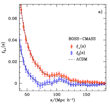
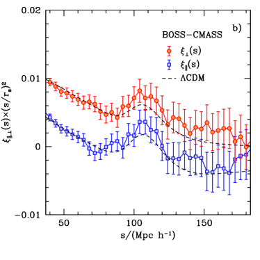
Panel a) of Fig. 1 shows the clustering wedges (circles) and (squares) of the CMASS sample obtained through the procedure described above. The dashed lines correspond to the best-fitting CDM model obtained from the combination of these measurements with CMB observations as described in Section 5.1.1. Panel b) of Fig. 1 displays the same measurements rescaled by the ratio , where corresponds to the sound horizon scale in our fiducial cosmology. The BAO peak can be clearly seen in both clustering wedges.
To obtain an estimate of the covariance matrix of the CMASS clustering wedges, we use the mock catalogues of Manera et al. (2012)111These mock catalogues are publicly available in http://www.marcmanera.net/mocks/. These are a set of independent mock catalogues corresponding to our fiducial cosmology, which are based on a method similar to PTHalos (Scoccimarro & Sheth, 2002) and were designed to follow the selection function of the CMASS sample in the northern and southern Galactic survey areas. We measured the clustering wedges of each mock catalogue using the same binning scheme as for the real data and the radial weights of equation (2). These measurements were used to obtain an estimate of the full covariance matrix C of the pair , that is, taking into account the covariance between the two clustering wedges. The error bars in Fig. 1 correspond to the square root of the diagonal entries in C.
We restrict our analysis of the full shape of the CMASS clustering wedges to , where the model described in Section 3 gives a good description of the results from our mock catalogues. We assume a Gaussian likelihood function of the form when comparing these measurements with theoretical predictions. The calculation of the value of a given model requires the knowledge of the inverse covariance matrix. As our estimation of C is inferred from our mock catalogues, its inverse, , provides a biased estimate of the true inverse covariance matrix (Hartlap et al., 2007). To correct for this bias we rescale the inverse covariance matrix as
| (3) |
where corresponds to the total number of bins in the pair, leading to a correction factor of approximately 0.87.
2.2 Additional data-sets
We combine the information encoded in the full shape of the clustering wedges with additional CMB, BAO and SN observations in order to improve the obtained cosmological constraints. Here we give a brief description of each additional dataset.
Our CMB dataset combines the measurements of the temperature and polarization fluctuations of the CMB from the nine-year of observations of the WMAP satellite (Bennett et al., 2012; Hinshaw et al., 2012) in the range , the South Pole Telescope (SPT, Keisler et al., 2011) for , and the Atacama Cosmology Telescope (ACT, Das et al., 2011) for . We follow the treatment of Hinshaw et al. (2012) and account for the effect of secondary anisotropies by including the contributions from the Sunyaev-Zel’dovich (SZ) effect, and Poisson and clustered point sources in the form of templates whose amplitudes are treated as nuisance parameters and marginalized over.
Our BAO dataset combines the results from independent BAO analyses based on angle-averaged clustering measurements at lower redshifts than the CMASS sample. These constrain the parameter combination , where
| (4) |
We use the results of Beutler et al. (2011), who obtained an estimate of from the large-scale correlation function of the 6dF Galaxy Survey (6dFGS, Jones et al., 2009), and the 2% distance measurement of obtained by Padmanabhan et al. (2012) and Xu et al. (2012) from the application of the reconstruction technique (Eisenstein et al., 2007) to the final SDSS-II LRG sample. We do not include the measurements of Blake et al. (2011) from the final WiggleZ Dark Energy Survey (Drinkwater et al., 2010) in our analysis given the significant overlap of the WiggleZ data with the CMASS sample.
We also include information from the type Ia supernovae (SN) compilation of Conley et al. (2011), which includes the high-redshift SN from the first three years of the Supernova Legacy Survey (SNLS). Conley et al. (2011) performed a detailed analysis of the systematic effects affecting this sample. We follow their recipe to take into account these systematic errors in our cosmological constraints, which requires the introduction of two additional nuisance parameters, and , related to the stretch-luminosity and colour-luminosity relationships. When quoting our cosmological constraints, the values of these parameters are marginalized over.
With the exception of Section 5.3, we use the CMASS clustering wedges in combination with our CMB dataset. We refer to this combination as CMB+. Our tightest constraints are obtained including also the additional BAO and SN data in our analysis.
In order to quantify the impact of the additional information contained in the clustering wedges with respect to the angle-averaged correlation function, we also compare the results obtained by means of the CMB+ combination with those obtained by replacing the clustering wedges with the CMASS monopole from Sánchez et al. (2012).
3 Modelling clustering wedges
In this section we describe our model of the full shape of the clustering wedges, taking into account the effects of non-linear evolution, redshift-space distortions and bias. In section 3.1 we describe a simple recipe to compute the first multipoles of . In section 3.2 we use this recipe to construct our model of the clustering wedges. In section 3.3 we test this model against our ensemble of mock catalogues and use these results to illustrate the way in which these measurements can be used to constrain and .
3.1 The anisotropic correlation function
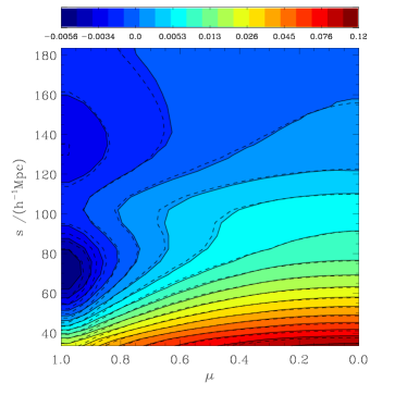
The clustering wedges and can be obtained by integrating over two wide bins of . Thus the starting point of our description of these measurements should be a model of the full two-dimensional correlation function. Figure 2 shows the mean redshift-space from our ensemble of mock catalogues (solid lines following the colour scheme). The effect of redshift-space distortions can be clearly seen in these contours, which strongly deviate from the horizontal lines that would correspond to the true underlying isotropic clustering. Although it is strongly affected by these distortions, the BAO feature is clearly noticeable at .
The anisotropic correlation function can be decomposed as a linear combination of Legendre polynomials, , as
| (5) |
where the multipoles are given by
| (6) |
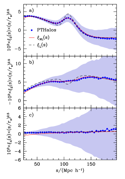
In practice, only a small number of multipoles of have non-negligible values on large scales. This can be seen in Figure 3, where the points correspond to the mean monopole (panel a), quadrupole (panel b), and hexadecapole (panel c) from our ensemble of mock catalogues. The shaded regions indicate the variance from the different realizations, corresponding to the uncertainties associated with one CMASS DR9 volume. To highlight the features on large scales these measurements have been rescaled by , where corresponds to the sound horizon at the drag redshift for our fiducial cosmology. The hexadecapole is consistent with zero over a wide range of scales and higher multipoles can be safely neglected. By modelling these multipoles, equation (5) can be used to describe the full .
In order to obtain a description of the multipoles , it is convenient to work with the two-dimensional power spectrum, . This quantity can also be decomposed in terms of Legendre polynomials, with multipoles given by
| (7) |
from which the multipoles can be obtained as
| (8) |
where is the spherical Bessel function of order (Hamilton, 1997).
In the linear perturbation theory regime, and assuming the distant observer approximation, the two-dimensional power spectrum can be described by the simple formula (Kaiser, 1987)
| (9) |
where is the linear-theory real-space power spectrum, is the bias factor, and , with , i.e., the logarithmic derivative of the growth factor . In this case all multipoles with vanish exactly. Even though this simple picture will be approximately valid when the amplitude of the density fluctuations is small, non-linear evolution introduces deviations from this behaviour (Smith et al., 2008; Crocce & Scoccimarro, 2008; Sánchez et al., 2008). This can be clearly seen in Figure 3, where the dashed lines correspond to the linear theory predictions for the multipoles . Although it is located at large scales, the differences in the appearance of the BAO signal are significant, as non-linear growth damps the BAO feature. This is particularly noticeable in the quadrupole, where the BAO signal is almost completely erased. These effects must be taken into account when attempting to extract precision cosmological information from these statistics.
Much work has been devoted over recent years to modelling the effects of non-linear evolution and redshift-space distortions. Pioneered by the work of Crocce & Scoccimarro (2006) on Renormalized Perturbation Theory (hereafter RPT), several new approaches to perturbation theory have been developed in recent years (e.g. Matsubara, 2008b, a; Matarrese & Pietroni, 2007, 2008; Pietroni, 2008; Taruya & Hiramatsu, 2008; Anselmi et al., 2011; Anselmi & Pietroni, 2012; Wang & Szalay, 2012). In these methods, the series expansion describing the power spectrum of standard perturbation theory is reorganized and some of the terms are re-summed into a function , usually called propagator, that can be factorized out of the series. The remaining terms contain mode-coupling contributions, , to the final non-linear power spectrum, which can then be written as . These approaches provide a better understanding of the effects of non-linear evolution on the shape of the two-point statistics, such as the power spectrum and the correlation function, in real-space. However, the extension of these results to the halo clustering in redshift space is somewhat more complicated. Although several recent studies have provided non-linear descriptions of redshift-space distortions for the matter and halo density fields (Scoccimarro, 2004; Tinker et al., 2006; Tinker, 2007; Matsubara, 2008b, a; Taruya et al., 2010, 2013; Jennings et al., 2011; Reid & White, 2011; de la Torre & Guzzo, 2012; Okumura et al., 2012), the range of validity of these models is limited and they rely on free parameters to fit the results from N-body simulations.
In this work we follow a simple approach and parametrize the non-linear two-dimensional power spectrum as
| (10) |
where
| (11) |
and , , and , are free parameters. Here is given by
| (12) |
where is the standard second order kernel of perturbation theory.
The description of the non-linear power spectrum of equation (11) is motivated by RPT. To a good approximation, the non-linear propagator is of Gaussian form, while, at large scales, equation (12) contains the leading order contribution to the full (see Crocce et al., 2012, for a more detailed description of these functions). The description of given by equation (11) is the basis of the parametrization of the non-linear correlation function proposed by Crocce & Scoccimarro (2008), and has been shown to give an accurate description of the power spectra and correlation functions measured from N-body simulations (e.g. Sánchez et al., 2008; Montesano et al., 2010) and real galaxy samples (Sánchez et al., 2009; Montesano et al., 2012; Beutler et al., 2011; Blake et al., 2011). In particular, this parametrization was used by Sánchez et al. (2012) to describe the CMASS monopole . The Lorentzian pre-factor in equation (10) represents a damping function which mimics the Finger-of-God effect corresponding to the assumption of an exponential galaxy velocity distribution function (Park et al., 1994; Cole et al., 1995).
The solid lines in Fig. 3 correspond to the multipoles obtained using the parametrization of equation (10), by fitting the free parameters in the model. These give an accurate description of the full shape of the mean monopole and quadrupole from our mock catalogues on large scales. On the other hand, while the shape of the mean hexadecapole from the mock catalogues is well described by the linear theory prediction, the results obtained from the parametrization of equation (10) only reproduce these measurements for scales larger than . These differences indicate the limitations of this model to describe the shape of the full anisotropic power spectrum . However, as we will see in Section 3.3, despite the simplicity of this recipe, its use as the basis of the modelling of the clustering wedges can provide unbiased cosmological constraints even for surveys probing volumes much larger than the SDSS-DR9 CMASS sample.
The monopole-quadrupole pair contains most of the information in the full plane. This can be seen in Fig. 2, where the dashed lines correspond to the contours of obtained by considering only the non-linear monopole and quadrupole terms of the multipole expansion of equation (5). These show a good agreement with the full measurement, describing most of its features. This result suggests that the monopole-quadrupole pair may contain the most relevant information for the description of the clustering wedges, a fact that we will exploit in the following section to construct a model for and .
3.2 From to the clustering wedges
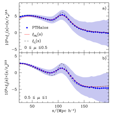
Figure 4 shows the mean clustering wedges (panel a) and (panel b) from our mock catalogues, rescaled by . The variance from the individual realizations is shown by the shaded region. The anisotropic clustering pattern generated by redshift-space distortions leads to significant differences in the amplitude and shape of the two clustering wedges, with showing a lower amplitude and a stronger damping of the BAO peak than . Here we use the description of the multipoles of the previous section to construct a model for the full shape of the clustering wedges.
The multipole description of can be used to compute the clustering wedges and . Discarding contributions from multipoles with , equation (1) implies that (Kazin et al., 2012)
| (13) | |||||
| (14) |
These equations demonstrate that the contribution from to the final clustering wedges is small and can be safely neglected.
The dashed lines in Fig. 4 correspond to the linear theory predictions for and . These are obtained using the multipoles in equations (13) and (14). Non-linear evolution causes the shape of the clustering wedges to deviate from these predictions, with the most notable differences at the scales of the BAO peak. The extraction of unbiased cosmological information from a measurement of the clustering wedges requires an accurate modelling of these distortions.
The solid lines in Figure 4 show the predictions for and obtained from equations (13) and (14) by considering the contributions from the multipoles with inferred from our model of the non-linear redshift-space power spectrum (equation 10). This simple recipe provides an accurate description of the full shape of the two clustering wedges, implying that the monopole-quadrupole pair contains the most relevant information required to describe these measurements.
3.3 Measuring and from the clustering wedges
As shown in Fig. 4, the model presented in Section 3.1 gives an accurate description of the full shape of the mean clustering wedges from our ensemble of mock catalogues. Here we test the ability of this model to recover unbiased cosmological constraints from these measurements by analysing the effect of the fiducial cosmology on and .
As described in Section 2.1, the measurement of the clustering wedges requires the assumption of a fiducial cosmology to map the observed redshifts into distances. This choice has a significant effect on the obtained results. Different fiducial cosmologies will lead to a rescaling of the components parallel and perpendicular to the line-of-sight, and , of the separation vector (Padmanabhan & White, 2008; Kazin et al., 2012; Xu et al., 2012). The relation between the true separations and those measured in the fiducial cosmology can be written as
| (15) | |||||
| (16) |
where the primes denote the quantities in the fiducial cosmology and the scaling factors are given by
| (17) | |||||
| (18) |
i.e., the ratios of the angular diameter distance and the Hubble parameter evaluated at the mean redshift of the survey, , in the true and fiducial cosmologies. Equations (15) and (16) are the basis of the Alcock–Paczynski test (Alcock & Paczynski, 1979). In terms of and , these equations can be written as
| (19) | |||||
| (20) |
These relations completely describe the impact of the fiducial cosmology on the clustering wedges, as they can be used to transform the integral in equation (1) from the fiducial cosmology space to the true cosmology as
| (21) |
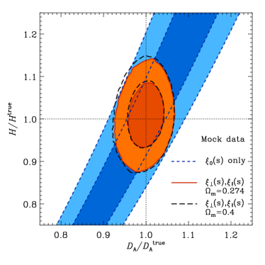
Equation (21) can be used to perform a simple test of the accuracy of our model of the clustering wedges. For this test we treat the parameters and in equations (19) and (20) as free parameters and fit for them using the mean clustering wedges from our mocks, while fixing all cosmological parameters to their true underlying values. As the fiducial cosmology used to obtain these measurements corresponds to the correct cosmology of the mocks, a deviation of the best fitting values of these parameters from would indicate a systematic bias in the model, which would then be unable to reproduce the correct shape of the clustering wedges. The result of this exercise is shown in Fig. 5, where the solid lines correspond to the 68 and 95 per cent two-dimensional marginalized constraints in the plane obtained in this way. These results have been marginalized over the fiducial parameters of the model, , , and . The values obtained in this case are and , showing that the model described in the previous sections gives an accurate description of the full shape of the clustering wedges, providing unbiased constraints on and .
As a further test of the ability of equations (19) and (20) to describe the effect of the fiducial cosmology on the clustering wedges we repeated this exercise, using the mean clustering wedges obtained from the same mock catalogues but assuming a different fiducial cosmology, with . The results obtained in this case are indicated by the long-dashed lines in Fig. 5. Despite the large difference between this fiducial cosmology and the true one of our mock catalogues, we recover the correct values of these parameters, with and . This exercise demonstrates that these equations can be used to describe the effect of the fiducial cosmology when comparing a given model with measurements of and .
For comparison, the short-dashed lines in Fig. 5 correspond to the constraints on and obtained from alone. These follow a degeneracy of constant , where is given by equation (4). The comparison of these constraints with the ones obtained from and clearly illustrates the extra information contained in the clustering wedges with respect of that of the monopole.
When dealing with clustering measurements obtained from observational data the true underlying cosmology is, of course, not known. Different cosmological models will predict different values of the acoustic scale . In this case, the angle-averaged correlation function provides constraints on the dimensionless quantity
| (22) |
Analogously, as shown by Kazin et al. (2012), the clustering wedges provide constraints on the parameter combinations
| (23) |
and
| (24) |
Therefore, when combined with a measurement of inferred from CMB observations, the clustering wedges can provide separate constraints on and .
4 Methodology
4.1 Cosmological parameter spaces
We explore similar sets of cosmological parameters as in Sánchez et al. (2012). Here we describe these parameter spaces and the methodology used to explore them.
We assume that primordial fluctuations are adiabatic, Gaussian, and have a power-law spectra of Fourier amplitudes, with a negligible tensor component. With these hypotheses a given cosmological model can be specified by the following sets of parameters,
| (25) |
These are the baryon and dark matter densities, and , the angular size of the sound horizon at recombination, , given by the ratio between the horizon scale at recombination and the angular diameter distance to the corresponding redshift, the curvature of the Universe, , the dark matter fraction in the form of massive neutrinos, , the dark energy equation of state parameter, . and the amplitude, , and spectral index, of the scalar primordial power spectrum, which we quote at the pivot wavenumber of .
We explore both the case of a constant dark energy equation of state and when it is allowed to vary with time, in which case we assume the standard linear parametrization of Chevallier & Polarski (2001) and Linder (2003) given by
| (26) |
where is the expansion factor and and are free parameters corresponding to the values of today and (minus) its derivative with respect to the scale factor, respectively.
The analysis of the CMB data requires an additional parameter, the optical depth to the last scattering surface, . This parameter is constrained by the CMB data alone and the inclusion of additional datasets leaves these results almost unchanged. As our CMB dataset was also used by Hinshaw et al. (2012), who present constraints on this parameter, we do not include them here.
The parameters of equation (25) allow us to derive constraints on other important quantities, such as
| (27) |
This set contains the dark energy and total matter densities, the sum of the neutrino masses, the Hubble parameter, the rms linear perturbation theory variance in spheres of radius , and the logarithmic derivative of the growth factor, . In Section 5.2.4 we explore the constraints on potential deviations from general relativity by treating as a free parameter, instead of computing its value as a derived quantity.
In Section 5.3 we explore the constraints on the geometrical quantities
| (28) |
given by equations (22)–(24). These parameters contain the combinations of the sound horizon at the drag redshift, , and the Hubble parameter, , angular diameter distance, , and average distance, , to the mean redshift of the sample.
The starting point of our analysis is the basic CDM parameter space which corresponds to a flat universe where the energy budget contains contributions from cold dark matter (CDM), baryons, and dark energy, described by . Our constraints on the CDM parameter space are described in Section 5.1.1. In Sections 5.1.2–5.2.4 we explore a number of possible extensions of this parameter space by allowing for variations on the remaining parameters of equations (25).
We explore these parameter spaces using the CosmoMC code of Lewis & Bridle (2002), which uses camb to compute power spectra for the CMB and matter fluctuations (Lewis et al., 2000). We use a generalized version of camb which supports a time-dependent dark energy equation of state (Fang et al., 2008). We included additional modifications from Keisler et al. (2011), Das et al. (2011) and Conley et al. (2011) to compute the likelihood of the SPT, ACT and SNLS datasets.
4.2 Testing the model of and
In section 3.3 we compared our model of and against the results from our mock catalogues in a simplified case, when the true underlying cosmology was known. Here we test the ability of the model to recover the true cosmological parameters under the same conditions in which we apply it to the CMASS measurements.
With the exception of Section 5.3, we use the clustering wedges in combination with our CMB dataset. The information provided by the CMB data can be well described using the following set of parameters (see e.g. Komatsu et al., 2009, 2011)
| (29) |
This set includes the redshifts of recombination, , the sound horizon at the drag redshift, , the CMB acoustic angular scale, , defined as
| (30) |
the shift parameter, , given by
| (31) |
the baryon density, and the amplitude and spectral index of the primordial scalar fluctuations. The redshift of recombination and the drag redshift are computed using the formulas of Eisenstein & Hu (1998).
A good approximation of the full CMB likelihood can be obtained from the best fitting values of the parameters of equation (29) and their covariance matrix . We use this parameter set to estimate the likelihood function of a mock CMB dataset, with equivalent characteristics to the real one, but corresponding to our fiducial cosmology, as with
| (32) |
where corresponds to the values of the parameters of equation (29) for our fiducial cosmology and is the corresponding covariance matrix inferred from our true CMB dataset. Using the approximated of equation (32) we can test our model of the clustering wedges by applying it to the mean and from our mock catalogues in combination with CMB data.
| CMB | CMB+ | CMB+ | CMB+ | |
| +BAO+SN | ||||
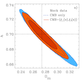
Panel a) of Fig. 6 shows the two-dimensional marginalized constraints in the – plane obtained when exploring the parameters of the CDM model using our mock CMB data (dashed lines), and its combination with the mean clustering wedges of our mock CMASS catalogues. The information in the clustering wedges alleviates the degeneracy in the CMB constraints, leading to a reduction of the allowed ranges of these parameters. In this case we find and , in excellent agreement with their true underlying values of and .
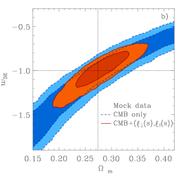
More stringent tests of our methodology can be obtained extending the parameter space by including as a free parameter, where degeneracies in the CMB data allow for significant deviations from the true cosmology. The results obtained in this case can be seen in Panel b) of Fig. 6, which shows the two-dimensional marginalized constraints in the – plane obtained from our mock CMB+CMASS dataset (solid lines). For this parameter space we find and . The allowed region for these parameters is centred in the correct underlying values, indicated by the dotted lines.
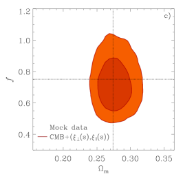
The model of the clustering wedges described in Section 3 depends on the value of the growth index . This fact offers the opportunity to obtain constraints on this quantity by treating it as a free parameter and checking its consistency with the value corresponding to GR. To test the performance of our model for the clustering wedges in this case, we explored the CDM parameter space extended by including as a free parameter. The solid lines in panel c) of Fig. 6 correspond to the two-dimensional marginalized constraints in the – plane obtained from the combination of our mock CMB and CMASS datasets. Also in this case the obtained constraints are in good agreement with the true underlying values for these cosmological parameters. We find , slightly lower than the fiducial value of but consistent within one .
The assumption that follows the predictions of GR has a significant impact on the constraints on . Under this assumption, the relative amplitude of the two clustering wedges, which depends on , contains information on , helping to constrain by reducing the CMB-only degeneracy that can be seen in the dashed lines of panel b) of Fig. 6. When is treated as a free parameter, this extra information is lost, leading to a degradation of the constraints. When both and are allowed to float, the constraints on the dark energy equation of state change to . Although a tail in the posterior distribution of this parameter shifts the mean value of this parameter towards lower values, its maximum is close to the true fiducial one, .
In Section 5.3 we focus on the constraints on the dimensionless parameter combinations and obtained from the clustering wedges in isolation, that is, without combining them with any other dataset. We explored the constraints on these quantities using the mean clustering wedges of our mock catalogues, marginalizing over the remaining cosmological parameters. In this case we obtain the constraints and . These results are in complete agreement with the values of these parameter combinations in our fiducial cosmology, of 8.87 and 11.92, respectively.
These tests show that the model of the clustering wedges described in Section 3 can be used as a tool to extract unbiased cosmological constraints from the clustering wedges of the CMASS sample.
5 Cosmological constraints
In this section we present the cosmological constraints obtained from the full shape of the CMASS clustering wedges and . Section 5.1 presents a summary of the results obtained on the CDM model and its extensions assuming that the dark energy component can be characterized by , while in Section 5.2 we explore more general models to obtain clues on the origin of the accelerated expansion of the Universe. Our results show the impact of replacing the information from the monopole correlation function by that of the clustering wedges. In the cases where is fixed, the information contained in is sufficient to obtain accurate constraints, with the clustering wedges providing only a slight improvement. When this assumption is relaxed, the extra information provided by the clustering wedges is more useful, leading to substantial improvements with respect to the results obtained by means of .
5.1 Dark energy as a cosmological constant
| CMB | CMB+ | CMB+ | CMB+ | |
| +BAO+SN | ||||
| Non-flat models | ||||
| Massive neutrinos | ||||
| (95% CL) | (95% CL) | (95% CL) | (95% CL) | |
| (95% CL) | (95% CL) | (95% CL) | (95% CL) | |
| Constant dark energy equation of state | ||||
| Dark energy and curvature | ||||
| Time-dependent dark energy equation of state | ||||
Here we investigate the impact of the clustering wedges on the constraints on the CDM parameter space and its extensions assuming that dark energy behaves as a cosmological constant, that is, keeping the dark energy equation of state parameter fixed to .
5.1.1 The CDM parameter space
Due to its ability to describe a wide variety of cosmological observations, the CDM model has become the standard cosmological model. Here we study the constraints on this parameter space obtained from the datasets described in Section 2. Table 1 lists the constraints obtained in this case from different dataset combinations.
With the inclusion of the new WMAP9 data, the CMB-only constraints on this parameter space have changed slightly from those of Sánchez et al. (2012). The preferred values of and show a shift of approximately 0.5 towards higher and lower values, respectively, with and . Although this parameter space is well constrained by the CMB data, including the CMASS monopole in the analysis substantially improves the obtained constraints by breaking the degeneracy between these parameters, leading to and . Replacing the information in the CMASS by that of the full shape of the clustering wedges leads to essentially identical results. The consistency between the constraints obtained in the CMB+ and CMB+ cases is a confirmation of the validity of the treatment of redshift-space distortions implemented in our modelling of the clustering wedges.
The best-fit CDM model to the CMB+ combination is shown by the dashed lines in Fig. 1. This model provides an excellent description of the full shape of both CMASS clustering wedges and, in particular, of the shape and location of their BAO features. This model implies a real-space bias factor of , in good agreement with the one inferred from the CMASS monopole, , and with the results of Nuza et al. (2012), who found a value of for this galaxy sample. Within this parameter space, and with the assumption of GR, the combination of the CMB data with our CMASS clustering measurements provides a constraint on the growth factor of . As we will see in Section 5.2.4, when is treated as a free parameter, the constraints obtained from the CMB+ combination are in agreement with this result.
Including the additional BAO and SN datasets provides an improvement on the constraints on this parameter space beyond the results found in the CMB+ case. Using the full dataset combination we obtain the constraints and . These results imply that, within the CDM model, the present-day dark energy density can be constrained to , and the current acceleration of cosmic expansion to , that is, at a 4 per cent accuracy.
5.1.2 Spatial Curvature
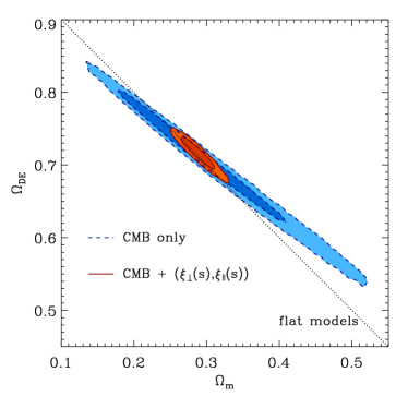
When the CDM parameter space is extended by allowing for non-flat models (i.e. ) the CMB-only constraints are significantly degraded due to the so-called geometric degeneracy (Efstathiou & Bond, 1999), corresponding to models with a constant CMB acoustic scale (given by equation 32). This degeneracy is shown by the dashed lines in Fig. 7, which correspond to the two-dimensional marginalized constraints in the – plane obtained using CMB information alone. The solid contours correspond to the results obtained when the CMB data is combined with the CMASS clustering wedges. The information in the shape of the clustering wedges breaks the geometrical degeneracy, providing much tighter constraints on these parameters. In this case we find the constraints and , in good agreement with a flat Universe.
As can be seen in Table 2, the CMB+ combination leads to a similar constraint than the one obtained in the CMB+ case, with and identical constraints on . This result demonstrates that the measurement of obtained from the monopole is sufficient to break the CMB degeneracies, with the extra information from the clustering wedges leading to similar constraints on .
Using the geometric constraints from the monopole-quadrupole of the same galaxy sample derived by Reid et al. (2012) in combination with the seven-year data of the WMAP satellite (WMAP7 Larson et al., 2011), Samushia et al. (2013) obtained the constraint . This value is consistent with our results from the CMB+ combination within 1, but points towards a larger deviation from a flat Universe. This difference can be traced back to the slightly higher value of found by Reid et al. (2012), which cuts the geometrical degeneracy of the CMB at a different location.
5.1.3 Neutrino mass
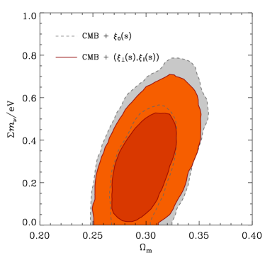
In this section we study how the constraints on the total neutrino mass change when using the information from the CMASS clustering wedges by exploring the CDM parameter space extended by including the neutrino fraction, , as a free parameter. A more detailed analysis of the constraints on neutrino masses inferred from the CMASS sample, paying special attention to the effects of the different priors and datasets used in the analysis, is presented in Zhao et al. (2012).
Fig. 8 shows the two-dimensional marginalized constraints in the – plane obtained by means of the CMB+ (dashed lines) and CMB+ (solid lines) dataset combinations. The use of the clustering wedges leads to a slight improvement on the constraints with respect to those obtained from the CMASS monopole. The CMB+ combination gives and (95 per cent CL). Replacing the angle-averaged correlation function by the clustering wedges leads to a slight improvement of the constraints, with and (95 per cent CL). These results imply a final limit on the sum of the neutrino masses of eV (95 per cent CL) for the CMB+ case and eV (95 per cent CL) when combining the CMB dataset with the CMASS clustering wedges. Including the additional BAO and SN information helps to improve these limits to and eV (95 per cent CL).
5.2 Understanding cosmic acceleration
In the previous sections we assumed that the dark energy component was given by vacuum energy or a cosmological constant, with . In this section we investigate alternative explanations of the observed accelerated expansion of the Universe by exploring constraints on the dark energy equation of state and its time evolution. As we will see, the constraints on these parameter spaces are substantially improved when the information from the CMASS monopole is replaced by that of the clustering wedges. We also analyse potential deviations from general relativity by exploring the constraints on the growth factor , which can only be obtained from anisotropic clustering measurements.
5.2.1 The dark energy equation of state
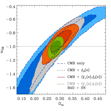
We start our exploration of more general dark energy models by extending the basic CDM parameter space by including the redshift-independent value of as a free parameter. In this case, the constraints derived from CMB data alone exhibit a strong degeneracy between and . This is illustrated by the long-dashed lines in Fig. 9, which correspond to the two-dimensional marginalized constraints on these parameters obtained from our CMB dataset. As shown in Sánchez et al. (2012), this degeneracy is partially broken when this information is combined with the CMASS monopole correlation function. Using this combination we find the marginalized constraints and , in agreement with the fiducial value of the CDM model but with significant room for alternative dark energy scenarios. The short-dashed lines in Fig. 9 correspond to the constraints in the plane obtained in this case, while the solid lines show the effect of replacing the information of the CMASS monopole by that of the full shape of the CMASS pair. This information is much more efficient at breaking the CMB degeneracy than , leading to a significant improvement of the obtained constraints. In this case we obtain and . These results, which are consistent with a cosmological constant at a one level, represent a reduction of the allowed range of these parameters by a factor two with respect to the ones obtained by means of the CMB+ combination.
Using the consensus anisotropic BAO measurements from the CMASS clustering wedges and multipoles, Anderson et al. (2013) found a constraint of , quite similar to the results obtained using the isotropic BAO results of Anderson et al. (2012). The comparison of this result with the ones from the CMB+ combination highlights the importance of using information from the full shape of the anisotropic clustering measurements to increase the information extracted from galaxy surveys. As we will see in Section 5.2.4, this extra information is degraded when is treated as a free parameter.
Our results are in excellent agreement with those derived from the full shape of the CMASS monopole-quadrupole pair in our companion paper Chuang et al. (2013), who find . Samushia et al. (2013) obtained the constraints and from the combination of the anisotropic clustering measurements of Reid et al. (2012) and WMAP7 data. By including smaller scales than in our analysis, with a different binning scheme, and imposing a stronger prior on the finger-of-god parameter , Reid et al. (2012) found slightly different, but consistent, geometrical constraints. These values cut the CMB-only degeneracy in a different region than our results, corresponding to slightly higher values or , with a smaller allowed range for this parameter.
5.2.2 Dark energy and curvature
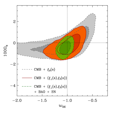
When the dark energy equation of state parameter and are varied simultaneously, the geometric degeneracy seen in the CMB-only results of Figs. 7 and 9 gains an extra degree of freedom, leading to poor constraints on both of these parameters. For this reason, the flatness hypothesis has strong implications on the derived constraints on the dark energy equation of state. In this section we explore how the constraints on are degraded if this assumption is relaxed.
The dashed lines in Fig. 10 show the two-dimensional marginalized constraints in the – plane obtained by combining our CMB dataset with the CMASS monopole. The information encoded in reduces the two-dimensional degeneracy obtained from the CMB data to an approximately one-dimensional degeneracy, which allows for values of significantly different from the CDM one, with . The solid contours in Fig. 10 correspond to the results obtained when the CMB data is combined with the CMASS clustering wedges. This dataset is much more efficient at breaking the degeneracy obtained from the CMB results, leading to a significant reduction of the allowed region of this parameter space, with the marginalized constraints and , in excellent agreement with the CDM model values, indicated by the dotted lines. Including the SN and additional BAO datasets improves the constraints even further, leading to and .
5.2.3 The time evolution of
In this section we study the constraints on the time evolution of , parametrized as in equation (26). Only by combining the CMB information with additional datasets it is possible to obtain meaningful constraints on these parameters.
| CMB+ | CMB+ | |||
| +BAO+SN | ||||
| – | – | |||
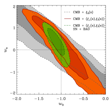
The dashed lines in Fig. 11 correspond to the two-dimensional marginalized constraints in the – plane obtained from the combination of our CMB dataset with the CMASS monopole. These results exhibit a strong degeneracy which spans the entire range of values allowed by our priors on these parameters. This degeneracy can be described by a linear combination of and , corresponding to the value of the dark energy equation of state at the pivot redshift , that is, the point where the uncertainty in is minimized. In this case we find . The solid lines in Fig. 11 correspond to the results obtained by combining the CMB data with the CMASS clustering wedges, showing a significant reduction of the allowed region for these parameters. In this case we find the marginalized limits and . As it is a common feature resulting from the parametrization of equation (26), the results obtained from the CMB+ combination also exhibit an approximately linear degeneracy between and , which corresponds to the constraint . The inclusion of the BAO and SN datasets tightens the constraints, leading to and , consistent with the CDM model.
The constraints obtained by means of different dataset combinations can be characterized by the Figure-of-Merit, FoM, defined as (Albrecht et al., 2006; Wang, 2008)
| (33) |
where corresponds to the covariance matrix of the parameters and . While the results obtained using the CMB+combination are described by , combining the CMB data with the CMASS clustering wedges instead leads to an increase of the FoM by nearly a factor two, with . This improvement clearly illustrates the importance of including anisotropic clustering measurements when constraining this parameter space. The final combination of all datasets leads to a further improvement by a factor four in the FoM, with .
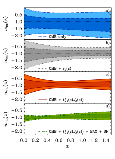
Our constraints on and can be translated into constraints on the value of as a function of . Fig. 12 shows the 68 and 95 per cent CL obtained using different dataset combinations. Although the CMB-only constraints (panel a) allow for significant deviations from , the inclusion of the CMASS restricts these variations, especially for (panel b). The result of combining the CMB data with the clustering wedges is shown in panel c). This dataset combination substantially reduces the allowed range of variations of . Panel d) shows the results obtained when the additional BAO and SN datasets are included in the analysis, which are completely consistent with the CDM model, showing no evidence of a deviation from the value at any redshift.
5.2.4 Constraining deviations from general relativity
The current phase of accelerated expansion of the Universe can be interpreted as the signature of a failure of general relativity to describe the behaviour of gravity on large scales. This scenario cannot be distinguished from that of a dark energy component solely on the basis of geometrical measurements. However, the combination of these tests with quantities sensitive to the growth of density fluctuations can break this degeneracy.
The model of the clustering wedges described in Section 3 depends on the value of , as it affects the pattern of redshift-space distortions in . As shown in Linder & Cahn (2007), in the context of general relativity the redshift evolution of this function can be well described by , with
| (34) |
In this way, assuming , a detection of a deviation from can be interpreted as the “smoking gun” of a failure of general relativity, as it would indicate that the growth of density fluctuations is not consistent with its predictions. In this section we explore the constraints obtained by treating as a free parameter, instead of using its derived value. By modelling the full shape of anisotropic clustering measurements, such as the clustering wedges, it is possible to combine the geometrical BAO test with a measurement of structure growth from the redshift-space distortions. Table 3 lists the constraints on the most relevant parameters obtained in this case, while a complete list can be found in Appendix A. This analysis is not possible when using angle-averaged measurements, where the effect of varying is completely degenerate with that of the bias parameter.
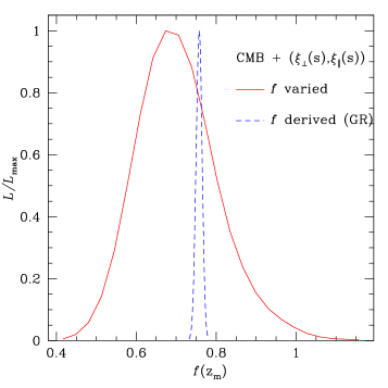
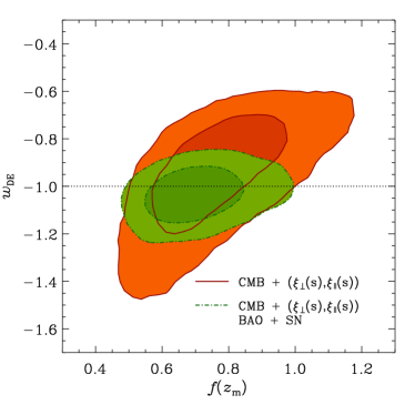
The solid line in Fig. 13 corresponds to the one-dimensional marginalized constraints on obtained from the CMB+ combination. In this case we obtain . Although a wide range of values of this parameter are allowed by the data, these results are consistent with the constraints derived when assuming GR in the context of the CDM model, which are shown by the dashed line and correspond to . The CMB+ result can be translated into a constraint of , consistent with the GR prediction of .
We also tested the effect of extending the CDM parameter space by allowing for simultaneous variations of (assumed time independent) and . Fig. 14 presents the two-dimensional marginalized constraints in the – plane obtained in this case by means of the CMB+ combination (solid lines), and when these data are combined with the BAO and SN datasets (dot-dashed lines). Including as a free parameter leads to a degeneracy between this quantity and the dark energy equation of state, degrading the constraints on these parameters. In this case we find and . As discussed in Section 4.2, assuming that follows the predictions of GR implies that the relative amplitude of and provides information on which improves the constraints. However, treating as a free parameter implies that this extra constraining powers is lost, leading to weaker constraints.
The effect of treating as a free parameter on the constraints on is general to all anisotropic clustering measurements, as it degrades the information on than can be extracted from the observed redshift-space distortions. This can be seen in the results of Samushia et al. (2013) and Chuang et al. (2013), who find that the the constraints on derived from the analysis of the CMASS – pair are affected in a similar way as those obtained from the clustering wedges.
Including the SN and additional BAO measurements breaks the degeneracy present in the CMB+ constraints, leading to and , similar to the ones derived when these parameters are varied separately and are in good agreement with the standard CDM+GR cosmological model.
5.3 Distance measurements
In this section we focus on the constraints on geometrical quantities obtained from the CMASS clustering wedges and their combination with our CMB dataset. Angle-averaged quantities such as the monopole provide constraints on the dimensionless quantity . However, as , this measurement represents a degeneracy between the angular diameter distance and the Hubble parameter which limits its power as a tool to derive cosmological constraints. As discussed in Section 3.3, the clustering wedges provide constraints on the parameter combinations and given by equations (23) and (24), breaking the degeneracy obtained from angle-averaged measurements.
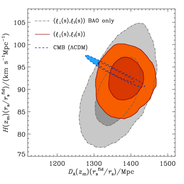
Using the full shape of the CMASS clustering wedges alone, and assuming that follows the predictions of GR, we obtain the constraints and , with a weak correlation coefficient of . The two-dimensional marginalized constraints on these quantities are shown by the solid lines in Fig. 15, where we have rescaled our results by the sound horizon at the drag redshift for our fiducial cosmology, , to express them in units of Mpc and . These results are in good agreement with the constraints obtained from a BAO-only analysis of the same CMASS clustering wedges in our companion paper Kazin et al. (2013), which are shown by the dot-dashed lines in the same figure. This comparison illustrates the additional constraining power of the full shape of and beyond that in the scale of the BAO peak alone. While a pre-reconstruction BAO-only analysis gives and , we obtain and .
The constraints on and obtained from the clustering wedges are degraded when is treated as a free parameter. In this case we find and . These results are in agreement with those of Chuang et al. (2013), who find and when fitting the full-shape of and while simultaneously varying , and .
Using the full shape of the CMASS angle-averaged correlation function, Sánchez et al. (2012) derived the constraint , in good agreement with the pre-reconstruction results of Anderson et al. (2012). From the analysis of the clustering wedges of this sample we find , showing that the same information is contained in the clustering wedges. The agreement between these results also provides a consistency test of the explicit treatment of redshift-space distortions implemented in our modelling of and .
The geometric constraints obtained from the clustering wedges are in agreement with those derived by Reid et al. (2012) from the full shape of the CMASS monopole-quadrupole pair. Using a WMAP7-based prior on the primordial power spectrum to calibrate the BAO ruler, Reid et al. (2012) found and . Applying a similar prior we find and , showing the consistency between our analysis techniques. By including smaller scales than in our analysis () and imposing a stronger prior on the finger-of-god parameter , Reid et al. (2012) found slightly different results than in our general analysis (i.e., without imposing a WMAP7 prior), but in agreement. This is the cause of many of the small differences in the cosmological constraints derived here and those of Samushia et al. (2013). When combined with CMB measurements, these geometric constraints cut the CMB degeneracies in slightly different regions, leading to distinct, but consistent, constraints.
The dashed lines in Fig. 15 correspond to the constraints obtained from our CMB dataset under the assumption of a CDM model. The results obtained from the clustering wedges are in good agreement with the predictions of the CDM model that best describes the CMB data. These results are a strong indication of the consistency of these datasets and their good agreement with the concordance CDM cosmological model.
When the clustering wedges are combined with CMB observations, the extra information leads to tighter constraints, with and . The information on provided by the CMB data makes it possible to derive direct constraints on the angular diameter distance and the Hubble parameter of and .
6 Conclusions
We have presented an analysis of the cosmological implications of the clustering wedges and , measured from the BOSS-DR9 CMASS sample. These statistics are defined by averaging the full two-dimensional correlation function, , over the ranges and , respectively. We apply a simple model of the full shape of these measurements in the mildly non-linear regime to derive constraints on the parameter combinations and , breaking the degeneracy between and obtained when using angle-averaged clustering measurements. We combine this information with additional cosmological probes, including CMB, SN, and BAO measurements from other datasets, to derive constraints on cosmological parameters. Our analysis is an extension of that of Sánchez et al. (2012) based on the monopole of the same galaxy sample analysed here. By comparing the constraints obtained from the clustering wedges with those derived by means of , we can quantify the impact of the extra information provided by the anisotropic clustering measurements.
Although using different measurements and modelling details, our results are in good agreement with those inferred from the full shape of the CMASS monopole-quadrupole pair by Reid et al. (2012), Samushia et al. (2013) and Chuang et al. (2013), and from the “consensus” anisotropic BAO measurements by Anderson et al. (2013), indicating the robustness of our results.
We find that the CDM model provides an excellent description of the full shape of the CMASS clustering wedges. When restricting our analysis to this parameter space, the CMB+ and CMB+ combinations give almost identical results. The consistency of the constraints obtained in these cases is a reassuring indication of the validity of the description of redshift-space distortions implemented in our modelling of the clustering wedges.
We explored a number of possible extensions of the CDM model. In some of these cases, such as when constraining non-flat models or the massive neutrino fraction while assuming that , the extra information in the clustering wedges only slightly improves the constraints with respect to those obtained by means of . However, this information proved to be most useful when allowing for deviations of the dark energy equation of state from the canonical CDM value. For example, when assuming a time-independent dark energy equation of state, using the CMB+ combination, we find . Instead, if the monopole is replaced by the clustering wedges, the allowed range for this parameter is reduced by a factor of two, leading to , consistent with a cosmological constant at a one level. Including also the BAO and SN datasets leads to the marginalized constraint , in excellent agreement with the CDM model.
When we explore the redshift dependence of the dark energy equation of state, parametrized as in equation (26), the CMB+ combination implies and , which can be translated into the constraint at the pivot redshift . These results represent an increase of the FoM by a factor of two with respect to the one found in the CMB+ case. Our final limit on these parameters is obtained from our full dataset combination, which shows no evidence for a redshift evolution of . In this case we find and and a constraint of at the pivot redshift .
As they are sensitive to the value of , the clustering wedges offer the opportunity to constrain potential deviations from the predictions of general relativity. This is not possible for angle-averaged clustering measurements, where is completely degenerate with the bias factor. If we extend the CDM model to include as a free parameter, we find . Assuming that this quantity behaves as our results imply a constraint of , consistent with no deviation from the GR prediction of .
The assumption that follows the predictions of GR implies that the relative amplitude of the clustering wedges contains information on . When is allowed to vary freely this additional constraining power is lost, affecting the constraints on other parameters. For example, if and are varied simultaneously, the CMB+ combination implies that and . However, when the additional BAO and SN measurements are included in the analysis we obtain and , with similar accuracies to the constraints derived when these parameters are varied independently and in good agreement with the standard CDM+GR cosmological model.
The geometric constraints on and from the clustering wedges are in perfect agreement with the best-fitting CDM model to the CMB data. This result shows the consistency between these datasets and with the standard cosmological model. Assuming the predictions of GR, using the information of the full shape of the clustering wedges we obtain and . These values are in good agreement with the pre-reconstruction results of Kazin et al. (2013), who used only the BAO signal in the same measurements, of and . The comparison of these results shows the effect of the extra information in the full shape of and beyond that encoded in the scale of the BAO peak.
Our results illustrate the extra constraining power of anisotropic clustering measurements with respect to that of angle-averaged quantities. The large volume and high number density of the CMASS DR9 sample make it possible to explore these measurements with a sufficiently high signal-to-noise ratio to derive meaningful cosmological constraints. By probing larger volumes, the galaxy samples from subsequent SDSS data releases will provide more accurate anisotropic clustering measurements. The availability of these new samples will be accompanied by the release of the CMB measurements from the Planck satellite. The combination of these datasets will undoubtedly push the achievable precision on our cosmological constraints to a new level, allowing us to put the CDM paradigm under even stricter scrutiny.
Acknowledgements
AGS acknowledges support by the Trans-regional Collaborative Research Centre TR33 ‘The Dark Universe’ of the German Research Foundation (DFG). EK is supported by the Australian Research Council Centre of Excellence for All-sky Astrophysics (CAASTRO), through project number CE110001020.
Numerical computations for the PTHalos mocks were done on the Sciama High Performance Compute (HPC) cluster which is supported by the ICG, SEPNet and the University of Portsmouth
Funding for SDSS-III has been provided by the Alfred P. Sloan Foundation, the Participating Institutions, the National Science Foundation, and the U.S. Department of Energy.
SDSS-III is managed by the Astrophysical Research Consortium for the Participating Institutions of the SDSS-III Collaboration including the University of Arizona, the Brazilian Participation Group, Brookhaven National Laboratory, University of Cambridge, Carnegie Mellon University, University of Florida, the French Participation Group, the German Participation Group, Harvard University, the Instituto de Astrofisica de Canarias, the Michigan State/Notre Dame/JINA Participation Group, Johns Hopkins University, Lawrence Berkeley National Laboratory, Max Planck Institute for Astrophysics, Max Planck Institute for Extraterrestrial Physics, New Mexico State University, New York University, Ohio State University, Pennsylvania State University, University of Portsmouth, Princeton University, the Spanish Participation Group, University of Tokyo, University of Utah, Vanderbilt University, University of Virginia, University of Washington, and Yale University.
We acknowledge the use of the Legacy Archive for Microwave Background Data Analysis (LAMBDA). Support for LAMBDA is provided by the NASA Office of Space Science.
References
- Ahn et al. (2012) Ahn C. P. et al., 2012, ApJS, 203, 21
- Aihara et al. (2011) Aihara H. et al., 2011, ApJS, 193, 29
- Albrecht et al. (2006) Albrecht A. et al., 2006, ArXiv Astrophysics e-prints
- Alcock & Paczynski (1979) Alcock C., Paczynski B., 1979, Nature, 281, 358
- Anderson et al. (2012) Anderson L. et al., 2012, MNRAS, 427, 3435
- Anderson et al. (2013) Anderson L. et al., 2013, submitted
- Anselmi et al. (2011) Anselmi S., Matarrese S., Pietroni M., 2011, J. Cosmol. Astropart. Phys., 6, 15
- Anselmi & Pietroni (2012) Anselmi S., Pietroni M., 2012, J. Cosmol. Astropart. Phys., 12, 13
- Bennett et al. (2012) Bennett C. L. et al., 2012, ArXiv e-prints
- Beutler et al. (2011) Beutler F. et al., 2011, MNRAS, 416, 3017
- Blake & Glazebrook (2003) Blake C., Glazebrook K., 2003, ApJ, 594, 665
- Blake et al. (2011) Blake C. et al., 2011, MNRAS, 418, 1707
- Bolton et al. (2012) Bolton A. S. et al., 2012, AJ, 144, 144
- Busca et al. (2012) Busca N. G. et al., 2012, ArXiv e-prints
- Cabré & Gaztañaga (2009) Cabré A., Gaztañaga E., 2009, MNRAS, 393, 1183
- Chevallier & Polarski (2001) Chevallier M., Polarski D., 2001, International Journal of Modern Physics D, 10, 213
- Chuang & Wang (2012) Chuang C.-H., Wang Y., 2012, MNRAS, 426, 226
- Chuang et al. (2013) Chuang et al., 2013, submitted
- Cole et al. (1995) Cole S., Fisher K. B., Weinberg D. H., 1995, MNRAS, 275, 515
- Cole et al. (2005) Cole S. et al., 2005, MNRAS, 362, 505
- Colless et al. (2001) Colless M. et al., 2001, MNRAS, 328, 1039
- Colless et al. (2003) Colless M. et al., 2003, ArXiv Astrophysics e-prints
- Conley et al. (2011) Conley A. et al., 2011, ApJS, 192, 1
- Crocce & Scoccimarro (2006) Crocce M., Scoccimarro R., 2006, Phys. Rev. D, 73, 063519
- Crocce & Scoccimarro (2008) Crocce M., Scoccimarro R., 2008, Phys. Rev. D, 77, 023533
- Crocce et al. (2012) Crocce M., Scoccimarro R., Bernardeau F., 2012, MNRAS, 427, 2537
- Das et al. (2011) Das S. et al., 2011, Physical Review Letters, 107, 021301
- Davis & Peebles (1983) Davis M., Peebles P. J. E., 1983, ApJ, 267, 465
- Dawson et al. (2013) Dawson K. S. et al., 2013, AJ, 145, 10
- de la Torre & Guzzo (2012) de la Torre S., Guzzo L., 2012, MNRAS, 427, 327
- Drinkwater et al. (2010) Drinkwater M. J. et al., 2010, MNRAS, 401, 1429
- Efstathiou & Bond (1999) Efstathiou G., Bond J. R., 1999, MNRAS, 304, 75
- Eisenstein & Hu (1998) Eisenstein D. J., Hu W., 1998, ApJ, 496, 605
- Eisenstein et al. (2005) Eisenstein D. J. et al., 2005, ApJ, 633, 560
- Eisenstein et al. (2007) Eisenstein D. J., Seo H.-J., Sirko E., Spergel D. N., 2007, ApJ, 664, 675
- Eisenstein et al. (2011) Eisenstein D. J. et al., 2011, AJ, 142, 72
- Fang et al. (2008) Fang W., Hu W., Lewis A., 2008, Phys. Rev. D, 78, 087303
- Frieman et al. (2008) Frieman J. A., Turner M. S., Huterer D., 2008, ARA&A, 46, 385
- Gaztañaga et al. (2009a) Gaztañaga E., Cabré A., Castander F., Crocce M., Fosalba P., 2009a, MNRAS, 399, 801
- Gaztañaga et al. (2009b) Gaztañaga E., Miquel R., Sánchez E., 2009b, Physical Review Letters, 103, 091302
- Gunn et al. (1998) Gunn J. E. et al., 1998, AJ, 116, 3040
- Gunn et al. (2006) Gunn J. E. et al., 2006, AJ, 131, 2332
- Hamilton (1997) Hamilton A. J. S., 1997, MNRAS, 289, 295
- Hartlap et al. (2007) Hartlap J., Simon P., Schneider P., 2007, A&A, 464, 399
- Hinshaw et al. (2012) Hinshaw G. et al., 2012, ArXiv e-prints
- Hu & Haiman (2003) Hu W., Haiman Z., 2003, Phys. Rev. D, 68, 063004
- Hütsi (2010) Hütsi G., 2010, MNRAS, 401, 2477
- Jennings et al. (2011) Jennings E., Baugh C. M., Pascoli S., 2011, MNRAS, 410, 2081
- Jones et al. (2009) Jones D. H. et al., 2009, MNRAS, 399, 683
- Kaiser (1987) Kaiser N., 1987, MNRAS, 227, 1
- Kazin et al. (2010) Kazin E. A. et al., 2010, ApJ, 710, 1444
- Kazin et al. (2012) Kazin E. A., Sánchez A. G., Blanton M. R., 2012, MNRAS, 419, 3223
- Kazin et al. (2013) Kazin et al., 2013, submitted
- Keisler et al. (2011) Keisler R. et al., 2011, ApJ, 743, 28
- Komatsu et al. (2009) Komatsu E. et al., 2009, ApJS, 180, 330
- Komatsu et al. (2011) Komatsu E. et al., 2011, ApJS, 192, 18
- Landy & Szalay (1993) Landy S. D., Szalay A. S., 1993, ApJ, 412, 64
- Larson et al. (2011) Larson D. et al., 2011, ApJS, 192, 16
- Lewis & Bridle (2002) Lewis A., Bridle S., 2002, Phys. Rev. D, 66, 103511
- Lewis et al. (2000) Lewis A., Challinor A., Lasenby A., 2000, ApJ, 538, 473
- Linder (2003) Linder E. V., 2003, Physical Review Letters, 90, 091301
- Linder & Cahn (2007) Linder E. V., Cahn R. N., 2007, Astroparticle Physics, 28, 481
- Maddox et al. (1990) Maddox S. J., Efstathiou G., Sutherland W. J., Loveday J., 1990, MNRAS, 242, 43P
- Manera et al. (2012) Manera M. et al., 2012, ArXiv e-prints
- Maraston et al. (2012) Maraston C. et al., 2012, ArXiv e-prints
- Masters et al. (2011) Masters K. L. et al., 2011, MNRAS, 418, 1055
- Matarrese & Pietroni (2007) Matarrese S., Pietroni M., 2007, J. Cosmol. Astropart. Phys., 6, 26
- Matarrese & Pietroni (2008) Matarrese S., Pietroni M., 2008, Modern Physics Letters A, 23, 25
- Matsubara (2004) Matsubara T., 2004, ApJ, 615, 573
- Matsubara (2008a) Matsubara T., 2008a, Phys. Rev. D, 78, 083519
- Matsubara (2008b) Matsubara T., 2008b, Phys. Rev. D, 77, 063530
- Meiksin et al. (1999) Meiksin A., White M., Peacock J. A., 1999, MNRAS, 304, 851
- Montesano et al. (2010) Montesano F., Sánchez A. G., Phleps S., 2010, MNRAS, 408, 2397
- Montesano et al. (2012) Montesano F., Sánchez A. G., Phleps S., 2012, MNRAS, 421, 2656
- Nuza et al. (2012) Nuza S. E. et al., 2012, ArXiv e-prints
- Okumura et al. (2008) Okumura T., Matsubara T., Eisenstein D. J., Kayo I., Hikage C., Szalay A. S., Schneider D. P., 2008, ApJ, 676, 889
- Okumura et al. (2012) Okumura T., Seljak U., Desjacques V., 2012, J. Cosmol. Astropart. Phys., 11, 14
- Padmanabhan et al. (2007) Padmanabhan N. et al., 2007, MNRAS, 378, 852
- Padmanabhan & White (2008) Padmanabhan N., White M., 2008, Phys. Rev. D, 77, 123540
- Padmanabhan et al. (2012) Padmanabhan N., Xu X., Eisenstein D. J., Scalzo R., Cuesta A. J., Mehta K. T., Kazin E., 2012, MNRAS, 427, 2132
- Park et al. (1994) Park C., Vogeley M. S., Geller M. J., Huchra J. P., 1994, ApJ, 431, 569
- Parkinson et al. (2012) Parkinson D. et al., 2012, Phys. Rev. D, 86, 103518
- Peebles & Ratra (2003) Peebles P. J., Ratra B., 2003, Reviews of Modern Physics, 75, 559
- Percival et al. (2001) Percival W. J. et al., 2001, MNRAS, 327, 1297
- Percival et al. (2007) Percival W. J., Cole S., Eisenstein D. J., Nichol R. C., Peacock J. A., Pope A. C., Szalay A. S., 2007, MNRAS, 381, 1053
- Percival et al. (2010) Percival W. J. et al., 2010, MNRAS, 401, 2148
- Percival et al. (2002) Percival W. J. et al., 2002, MNRAS, 337, 1068
- Pietroni (2008) Pietroni M., 2008, J. Cosmol. Astropart. Phys., 10, 36
- Reid et al. (2010) Reid B. A. et al., 2010, MNRAS, 404, 60
- Reid et al. (2012) Reid B. A. et al., 2012, MNRAS, 426, 2719
- Reid & White (2011) Reid B. A., White M., 2011, MNRAS, 417, 1913
- Ross et al. (2013) Ross A. J. et al., 2013, MNRAS, 428, 1116
- Ross et al. (2012) Ross A. J. et al., 2012, MNRAS, 424, 564
- Samushia et al. (2013) Samushia L. et al., 2013, MNRAS, 429, 1514
- Sánchez et al. (2008) Sánchez A. G., Baugh C. M., Angulo R. E., 2008, MNRAS, 390, 1470
- Sánchez et al. (2006) Sánchez A. G., Baugh C. M., Percival W. J., Peacock J. A., Padilla N. D., Cole S., Frenk C. S., Norberg P., 2006, MNRAS, 366, 189
- Sánchez et al. (2009) Sánchez A. G., Crocce M., Cabré A., Baugh C. M., Gaztañaga E., 2009, MNRAS, 400, 1643
- Sánchez et al. (2012) Sánchez A. G. et al., 2012, MNRAS, 425, 415
- Scoccimarro (2004) Scoccimarro R., 2004, Phys. Rev. D, 70, 083007
- Scoccimarro & Sheth (2002) Scoccimarro R., Sheth R. K., 2002, MNRAS, 329, 629
- Seo et al. (2012) Seo H.-J. et al., 2012, ApJ, 761, 13
- Shoji et al. (2009) Shoji M., Jeong D., Komatsu E., 2009, ApJ, 693, 1404
- Smee et al. (2012) Smee S. et al., 2012, ArXiv e-prints
- Smith et al. (2008) Smith R. E., Scoccimarro R., Sheth R. K., 2008, Phys. Rev. D, 77, 043525
- Spergel et al. (2007) Spergel D. N. et al., 2007, ApJS, 170, 377
- Taruya & Hiramatsu (2008) Taruya A., Hiramatsu T., 2008, ApJ, 674, 617
- Taruya et al. (2013) Taruya A., Nishimichi T., Bernardeau F., 2013, ArXiv e-prints
- Taruya et al. (2010) Taruya A., Nishimichi T., Saito S., 2010, Phys. Rev. D, 82, 063522
- Tegmark et al. (2004) Tegmark M. et al., 2004, ApJ, 606, 702
- Tinker (2007) Tinker J. L., 2007, MNRAS, 374, 477
- Tinker et al. (2006) Tinker J. L., Weinberg D. H., Zheng Z., 2006, MNRAS, 368, 85
- Tojeiro et al. (2012) Tojeiro R. et al., 2012, MNRAS, 424, 2339
- Wagner et al. (2008) Wagner C., Müller V., Steinmetz M., 2008, A&A, 487, 63
- Wang & Szalay (2012) Wang X., Szalay A., 2012, Phys. Rev. D, 86, 043508
- Wang (2008) Wang Y., 2008, Phys. Rev. D, 77, 123525
- White et al. (2011) White M. et al., 2011, ApJ, 728, 126
- Xu et al. (2012) Xu X., Padmanabhan N., Eisenstein D. J., Mehta K. T., Cuesta A. J., 2012, MNRAS, 427, 2146
- York et al. (2000) York D. G. et al., 2000, AJ, 120, 1579
- Zhao et al. (2012) Zhao G.-B. et al., 2012, ArXiv e-prints
Appendix A Summary of the obtained constraints on extensions of the CDM model
In this appendix we summarize the constraints on cosmological parameters obtained using different combinations of the datasets described in Section 2. Tables 4-9 list the 68% confidence limits obtained in the extensions of the CDM parameter space analysed in Sections 5.1.2 to 5.2.4. The upper section of these tables lists the constraints on the main parameters (equation 25) included in the fits, while the lower section contains the results on the parameters derived from this set (equation 27).
| CMB | CMB+ | CMB+ | CMB+ | |
|---|---|---|---|---|
| +BAO+SN | ||||
| CMB | CMB+ | CMB+ | CMB+ | |
| +BAO+SN | ||||
| (95% CL) | (95% CL) | (95% CL) | (95% CL) | |
| (95% CL) | (95% CL) | (95% CL) | (95% CL) | |
| CMB | CMB+ | CMB+ | CMB+ | |
|---|---|---|---|---|
| +BAO+SN | ||||
| CMB | CMB+ | CMB+ | CMB+ | |
|---|---|---|---|---|
| +BAO+SN | ||||
| CMB | CMB+ | CMB+ | CMB+ | |
|---|---|---|---|---|
| +BAO+SN | ||||
| CMB+ | CMB+ | |||
|---|---|---|---|---|
| +BAO+SN | ||||
| – | – | |||