Joint Minkowski Functionals and Bispectrum Constraints on Non-Gaussianity in the CMB

Abstract

Two of the most commonly used tools to constrain the primordial non-Gaussianity are the bispectrum and the Minkowski functionals of CMB temperature anisotropies. These two measures of non-Gaussianity in principle provide distinct (though correlated) information, but in the past constraints from them have only been loosely compared and not statistically combined. In this work we evaluate, for the first time, the covariance matrix between the local non-Gaussianity coefficient $f_{\rm NL}$ estimated through the bispectrum and Minkowski functionals. We find that the estimators are positively correlated, with correlation coefficient $r\simeq 0.3$. Using the WMAP7 data to combine the two measures and accounting for the point-source systematics, we find the combined constraint $f_{\rm NL}=37\pm 28$, which has a $\sim 20\%$ smaller error than either of the individual constraints.

I Introduction

Detection of any departures from Gaussianity in the distribution of primordial fluctuations would give important information about inflation. Primordial non-Gaussianity (henceforth NG) imprints signatures on the cosmic microwave background (CMB) and large-scale structure, and these cosmological probes can in turn provide excellent constraints on primordial NG and thus inflationary models; for reviews, see Komatsu (2010); Bartolo et al. (2004); Liguori et al. (2010); Yadav and Wandelt (2010).

Two of the principal statistics on the CMB used to constrain NG are the bispectrum (harmonic transform of the three-point correlation function) of the CMB temperature fluctuations, and Minkowski functionals (henceforth MF) which roughly measure the connectedness or morphology of the CMB field. In the “local” model of NG, the primordial curvature perturbation $\Phi(\bf{x})$ has a quadratic term correction: $\Phi=\Phi_{G}+f_{\rm NL}(\Phi_{G}^{2}-\langle\Phi_{G}^{2}\rangle)$, where $\Phi_{G}$ is an auxiliary Gaussian field Komatsu and Spergel (2001). Recent constraints obtained on the non-linear coupling constant $f_{\rm NL}$ using the WMAP data are $f_{\rm NL}=37\pm 20$ from the bispectrum analysis Bennett et al. (2012) (see also Yadav and Wandelt (2008); Smith et al. (2009)), and $f_{\rm NL}=20\pm 42$ from the MF analysis Hikage and Matsubara (2012).

Since MF are morphological statistics, they probe NG both in configuration space and to all orders of the statistics of the temperature anisotropy field. This means that they sample the anisotropy map differently from the usual bispectrum (and higher order polyspectra) measurements, albeit in a suboptimal way – this fact is crucial as joint constraints will in principle yield different constraints. Furthermore, unlike the bispectrum estimators which require a template (i.e. $k$-space configuration with a free amplitude) such as the local, equilateral or orthogonal type, MF are in principle template-free, although in practice one can construct a template-based MF estimator as we have done in this paper.

In principle, the MF are sensitive to the weighted sum of the bispectrum coefficients (out to the smallest scale measured) Hikage et al. (2006), so the MF would naively be expected to contain only a subset of the same information as the bispectrum. In reality, however, this idealized expectation is not borne out: the bispectrum and the MF partially complement each other, and their information is not 100% correlated. One reason for this is the fact that the optimal bispectrum estimators Babich (2005); Creminelli et al. (2006) are computationally challenging to implement for current high-precision CMB experiments Smith et al. (2009); Ade et al. (2013), and they are anyway only optimal for the case of vanishing non-Gaussianity Creminelli et al. (2007); Liguori et al. (2007). Moreover, the bispectrum and MF are sensitive to different astrophysical and analysis-related systematics, given that they are defined in the harmonic and real space respectively. Hence, combining the constraints obtained by current fast though sub-optimal bispectrum estimators with those from the MF, as we do in this paper, provides an alternative to improving the “optimality” of these estimators, and makes the combined constraints both stronger and more robust.

Hence an obvious question is how correlated are the MF and the bispectrum estimators, and consequently what is the combined constraint on NG from them. This is the question that we address in this paper – we will show that the correlation between the two estimators, while nonzero, is far from maximal. Having calculated that, we compute the joint estimate of NG from both statistics.

II Minkowski functionals methodology

The three Minkowski functionals $V_{i}\ (i=0,1,2)$ describe morphological properties of the hot and cold spots in the CMB temperature map. The morphology of the map, and thus the MF, are studied by specifying a temperature threshold $\nu\equiv(\Delta T/T)/\sigma_{0}$ in the map, where $\sigma_{0}$ is the rms of the fractional temperature fluctuation $\Delta T/T$, hereafter simply denoted as $f$. Specifically, $V_{0}$ is the area fraction of the regions above the temperature threshold, $V_{1}$ is their boundary length, and $V_{2}$ is the geodesic curvature integrated along their boundary, which in a compact $S_{2}$ space is related to the Euler characteristic $\chi$ by $\chi=V_{2}+V_{0}/2\pi$ Schmalzing and Gorski (1998). The MF can be expressed as integrals of functions of the anisotropy field and its derivatives over the compact space of the CMB sky. For explicit expressions see e.g. Schmalzing and Gorski (1998); Hikage et al. (2006); we shall adopt these operationally convenient forms to calculate the MF for a given map.

If the temperature fluctuations are Gaussian, the ensemble averages of the Minkowski functionals have analytic expressions that are completely specified by the two-point statistics (variance) of the fluctuations, $\sigma_{0}^{2}$ and $\sigma_{1}^{2}(\equiv\langle|\nabla f|^{2}\rangle)$ Tomita (1986). On the other hand, when the fluctuations are weakly non-Gaussian and the cumulants $\langle f^{n}\rangle_{c}$ (where “c” stands for the connected part) satisfy the hierarchical ordering $\langle f^{n}\rangle_{c}\sim\sigma_{0}^{2n-2}$, one can obtain an order-by-order expansion in powers of $\sigma_{0}$ for the average of the Minkowski functionals Matsubara (2003, 2010). In this letter, we consider the first order in the hierarchical non-Gaussian expansion, which in addition to $\sigma_{0}$ and $\sigma_{1}$ depends on the three-point statistics (skewness) of the field: $S\equiv\langle f^{3}\rangle,\ S_{I}\equiv\langle f^{2}\nabla^{2}f\rangle,\ S_{II}\equiv 2\langle|\nabla f|^{2}\nabla^{2}f\rangle$. The two variance and the three skewness parameters can be calculated from theory by integrating over the power spectrum and bispectrum of the CMB field, respectively; for explicit expressions, see Hikage et al. (2006); Hikage and Matsubara (2012). In the special case of the local-type primordial non-Gaussianity, $S,\,S_{I},\,S_{II}$ are all linearly proportional to $f_{\rm NL}$.

In this Letter, we use the co-added V+W band data from the WMAP seven-year results Komatsu et al. (2011) to obtain our constraints on $f_{\rm NL}$. The V and W bands are chosen for they are the most foreground-free. For this purpose, we generate 1000 simulations of the WMAP data following the procedure given in Appendix A of Komatsu et al. (2009). The only difference (aside from using the WMAP7 cosmological model) is that we used a uniform weighting for the maps, rather than the slightly more complicated weighting given there, since it only gives a marginal improvement in estimating $f_{\rm NL}$. Each of our simulated map is the sum of three components: 1) the Gaussian CMB realizations (the “signal”) based on the CMB power spectrum calculated assuming the best-fit WMAP seven-year cosmology including the effect of beam smearing, 2) instrumental noise modeled as the Poisson process with the rms noise per pixel $\sigma/\sqrt{N_{\rm obs}}$, where $\sigma$ is the rms noise per observation and $N_{\rm obs}$ is the number of observations per pixel, and 3) unresolved point sources modeled as the Poisson realizations from assuming a single population of sources with a fixed frequency-independent flux whose flux strength and number density roughly reproduce the source power spectrum and bispectrum measured from the WMAP Q band. The latter two components are modeled to closely match the systematics expected in the V+W co-added map. We then mask both the WMAP data and our simulated maps by using the KQ75 mask.

To make predictions for the ensemble average of the Minkowski functionals when various observational effects are present, we should also include these effects in the calculations of the two variance parameters and three skewness parameters. Each of these parameters has contributions from the noise part – instrumental noise and point sources, in addition to the beam-smeared CMB signal part. The noise and signal contributions add up directly since the CMB signal and noise are uncorrelated. We estimate these noise contributions from our simulations: we calculate the variance and skewness parameters for each simulated map, and take their average over the 1000 samples; we then subtract off the signal contributions which are known to us for these Gaussian CMB simulations.

Before we proceed to the fitting procedure and obtain our Minkowski functional constraints on $f_{\rm NL}$, we address the “residual problem” in our numerical evaluation of the Minkowski functionals. Previous work Hikage et al. (2008) found that, even for a set of Gaussian CMB simulations without noise, the averages of the MF calculated for each map are different from their values expected from theory. As shown in Lim and Simon (2012), these residuals are generated by the discrete binning of the MF in the threshold $\nu$, and for weakly non-Gaussian maps can be calculated analytically and then subtracted order by order in $\sigma_{0}$. In this work, we instead follow Hikage et al. (2008) and calculate the residuals from our simulations as the difference of the sample-averaged means of the MF and their theoretically expected means. These residuals are then subtracted from the measured Minkowski functionals. We use the same residuals to account for those for the non-Gaussian case: for a weakly non-Gaussian field, the differences are at the order of $\sigma_{0}$.

Before we calculate the Minkowski functionals for each map, we smooth the map at several different angular scales. This allows us to extract additional information from the map and tighten the constraints on $f_{\rm NL}$. Specifically, we use a Gaussian window function, and smooth each map at five different scales with the Full Width Half Maximum (FWHM) $\theta$ set at $\theta=10^{\prime},\ 20^{\prime},\ 40^{\prime},\ 80^{\prime},\ 100^{\prime}$. Pixels within a distance of $\theta$ away from the boundary of the KQ75 mask are removed to avoid contamination from the masked regions that may be introduced due to the smoothing. Ideally, one may want to smooth the maps at infinitely many scales and extract the constraint on $f_{\rm NL}$ by integrating over them. Clearly, this cannot be done in reality. The five smoothing scales we choose range from roughly the resolution of the WMAP V+W band data to the scale at which only $\sim 40\%$ of the map remains for analysis. (Note, the larger the smoothing scale, the bigger the area to be removed to avoid contamination.) Combining the results at the five smoothing scales allows us to recover most of the available information. For each smoothed map, we calculate its three Minkowski functionals at 15 temperature thresholds from $\nu=-3.5$ to $3.5$ with equal bin size of $\Delta\nu=0.5$.

To obtain the constraints on $f_{\rm NL}$, we perform a $\chi^{2}$ analysis, which compares theoretical predictions at a given $f_{\rm NL}$ to the measurements, and is calculated as

$$\chi^{2}=\sum_{i,j}\left[V_{i}^{\rm obs}-V_{i}^{\rm th}(f_{\rm NL})\right]C^{-1}_{ij}\left[V_{j}^{\rm obs}-V_{j}^{\rm th}(f_{\rm NL})\right],$$ (1)

where $i$ and $j$ run over all combinations of the 15 thresholds, three orders, and five smoothing scales for the measured Minkowski functionals. Here $V_{i}^{\rm obs}$ are the “observed” numerically evaluated Minkowski functionals, $V_{i}^{\rm th}$ are the theoretically expected averages for the MF (which are functions of $f_{\rm NL}$), and $C$ is the covariance matrix for $(V_{i},V_{j})$ which we calculate from our simulations as

$$C_{ij}=\langle\left(V_{i}-\langle V_{i}\rangle\right)\left(V_{j}-\langle V_{j}\rangle\right)\rangle_{\rm sim},$$ (2)

where the angular brackets denote averaging over the 1000 simulated maps. We then obtain our best-fit value of $f_{\rm NL}$, henceforth $f_{\rm NL}^{\rm MF}$, by minimizing the $\chi^{2}$.

To check that our estimator for $f_{\rm NL}^{\rm MF}$ is unbiased, we first apply it to the 1000 simulated maps either for the MF measurements at each smoothing scale or their combined results. We find that the average of the best-fit values accurately reproduces the theoretical input in our simulation, i.e., $f_{\rm NL}=0$. Next, we test our estimator on publicly available non-Gaussian CMB maps generated with the local-type NG Elsner and Wandelt (2009), and we again find negligible bias (1% or less of the true $f_{\rm NL}$) in our estimator.

	$\theta(^{\prime})$		$f_{\rm NL}$
	10	$\,71\!\!\!\!\!$	$\pm$	$\!\!\!\!\!96\,$
Minkowski	20	$-21\!\!\!\!\!$	$\pm$	$\!\!\!\!\!52$
Functionals	40	$-2\!\!\!\!\!$	$\pm$	$\!\!\!\!\!49$
	80	$\,40\!\!\!\!\!$	$\pm$	$\!\!\!\!\!73\,$
	100	$\,-16\!\!\!\!\!$	$\pm$	$\!\!\!\!\!92\,$
	all	$29\!\!\!\!$	$\pm$	$\!\!\!\!\!33$
bispectrum		$46\!\!\!\!\!\!$	$\pm$	$\!\!\!\!\!35$
MF + bisp		$\bf{37}\!\!\!\!\!\!$	$\bf{\pm}$	$\!\!\!\!\!{\bf{28}}$

Table 1: Constraints on $f_{\rm NL}$ from the CMB Minkowski functionals, bispectrum, and their combination. The analyses use the WMAP 7-year V+W co-added map. $\theta$ is the FWHM of the Gaussian beam used to smooth the map for the Minkowski functional analysis.

Finally, we apply our estimator on the co-added V+W band data from the WMAP. In Table 1, we show the constraints on $f_{\rm NL}^{\rm MF}$ from smoothing the map at each of the five angular scales, and the joint constraint from all scales combined, which we quote as our final MF constraint: $f_{\rm NL}^{\rm MF}=29\pm 33$. This constraint is consistent with that found by Hikage & Matsubara Hikage and Matsubara (2012), although we improve upon their analysis in a couple of ways: 1) we remove the residuals in the numerically evaluated MFs using the method from Hikage et al. (2008), as opposed to the residual removal based on the work in Lim and Simon (2012) which, we found, causes biases in the estimated $f_{\rm NL}^{\rm MF}$ by $\sim 10$. and 2) we carefully include point sources in our simulated WMAP maps.

III Bispectrum methodology

With the MF estimator of $f_{\rm NL}^{\rm MF}$ obtained, we next develop $f_{\rm NL}^{\rm bisp}$ – the estimator from bispectrum. The observed CMB bispectrum is given by

$$B_{\ell_{1}\ell_{2}\ell_{3}}=\sum_{m_{1}m_{2}m_{3}}\left(\begin{array}[]{ccc}\!\ell_{1}\!&\ell_{2}\!&\ell_{3}\!\\ \!m_{1}\!&m_{2}\!&m_{3}\!\end{array}\right)a_{\ell_{1}m_{1}}a_{\ell_{2}m_{2}}a_{\ell_{3}m_{3}},$$ (3)

where the matrix is the Wigner-3j symbol, and $a_{\ell m}$ is the spherical harmonic transform of the temperature anisotropy map. In the local-type NG model, $B_{\ell_{1}\ell_{2}\ell_{3}}$ is linearly proportional to $f_{\rm NL}$.

We follow the prescription that uses the KSW Komatsu et al. (2005) estimator to calculate $f_{\rm NL}^{\rm bisp}$ from CMB maps (see also Becker and Huterer (2012) for the exact implementation that we use). In brief, the KSW is a cubic (in the temperature field) estimator of non-Gaussianity; it is nearly minimum-variance and computationally fast, and can straightforwardly deal with partial sky coverage and inhomogeneous noise. The first ingredient in using KSW is to calculate the Fisher matrix $F$ corresponding to $f_{\rm NL}$; for this we need the theoretical bispectrum $B^{\rm theory}_{\ell_{1}\ell_{2}\ell_{3}}$ which can be calculated with the help of transfer functions from CAMB Lewis et al. (2000). Furthermore, KSW requires filtered maps $A(\mathbf{\hat{n}},r)$ and $B(\mathbf{\hat{n}},r)$ from which the skewness $S$ of the field can be calculated; these filtered maps can be computed using HEALPix (by way of HealPy) to perform the forwards and backwards spherical harmonic transforms that are necessary in their computation. Given the skewness and the Fisher matrix, the KSW estimator for $f_{\rm NL}$ is

$$f_{\rm NL}^{\rm bisp}={S\over F}.$$ (4)

To account for the masking of the CMB sky, we make the substitution $S\rightarrow S_{\rm cut}=S/f_{\rm sky}+S_{\rm linear}$ Yadav et al. (2008). $S_{\rm linear}$ is an addition to skewness and is calibrated to account for partial-sky observations

$$S_{\rm linear}= -{1\over f_{\rm sky}}\int r^{2}dr\int d^{2}\mathbf{\hat{n}}\left[A(\mathbf{\hat{n}},r)\langle B_{\rm sim}^{2}(\mathbf{\hat{n}},r)\rangle_{\rm MC}\right.$$

$$\left.+2B(\mathbf{\hat{n}},r)\langle A_{\rm sim}(\mathbf{\hat{n}},r)B_{\rm sim}(\mathbf{\hat{n}},r)\rangle_{\rm MC}\right].$$ (5)

The subscripted filtered maps $A_{\rm sim}$ and $B_{\rm sim}$ are created from Python-produced Gaussian Monte Carlo realizations of the cut CMB sky; the brackets $\langle\rangle_{\rm MC}$ indicate an average over 300 of the maps. The simulated maps were produced as outlined earlier when we discussed the MF.

Applying the bispectrum/KSW estimator to the co-added V+W band data of the WMAP, we obtain the constraint on the local NG to be $f_{\rm NL}^{\rm bisp}=46\pm 35$. The error we obtained is larger than that from Ref. Komatsu et al. (2011) using the same data because we have used a bispectrum estimator that is less optimal but much more convenient to evaluate.

IV Combined analysis

In addition to obtaining the constraints on $f_{\rm NL}$ separately from the MF and bispectrum analyses, we would like to combine them to extract a more stringent and robust result. To make the problem tractable, we opt to consistently combine the estimators of $f_{\rm NL}$ from these two analyses, rather than attempting to find the covariance between the observables, i.e. the MF and bispectrum themselves. It is a reasonably good assumption that the two estimators of $f_{\rm NL}$ satisfy a bivariate Gaussian distribution, especially near the peak of the distribution (see Figure 1 below). Let us organize the two estimators into a row-vector ${\bf f_{\rm NL}}\equiv[f_{\rm NL}^{\rm MF},\,f_{\rm NL}^{\rm bisp}]$, and let ${\bf C}$ be the $2\times 2$ covariance matrix for them. Assuming the underlying true value of $f_{\rm NL}$ is $\bar{f}_{\rm NL}$, we can write down the following joint-distribution for the two $f_{\rm NL}$ estimators

$$\mathcal{L}\propto|{\bf C}|^{-1/2}\exp\left[-{1\over 2}({\bf f_{\rm NL}-\bar{f}_{\rm NL}}){\bf C}^{-1}({\bf f_{\rm NL}-\bar{f}_{\rm NL}})^{T}\right],$$ (6)

where ${\bf\bar{f}_{\rm NL}}=[\bar{f}_{\rm NL},\,\bar{f}_{\rm NL}]\equiv\bar{f}_{\rm NL}\,\mathbb{I}$. Given a measurement of ${\bf f_{\rm NL}}$, a best estimate for $\bar{f}_{\rm NL}$ can be obtained by maximizing $\mathcal{L}$. Assuming that the covariance matrix does not depend on $\bar{f}_{\rm NL}$, we find the following expressions for the best estimate and variance of $\bar{f}_{\rm NL}$ from the combined analysis

$$\bar{f}_{\rm NL}=\frac{\mathbb{I}\,{\bf C}^{-1}\,{\bf f_{\rm NL}}^{T}}{\mathbb{I}\,{\bf C}^{-1}\,\mathbb{I}^{T}},\quad\sigma^{2}_{\bar{f}_{\rm NL}}=\frac{1}{\mathbb{I}\,{\bf C}^{-1}\,\mathbb{I}^{T}}.$$ (7)

At the same time, by evaluating both $f_{\rm NL}^{\rm MF}$ and $f_{\rm NL}^{\rm bisp}$ for the 1000 simulated WMAP maps, we numerically obtain their joint distribution, as shown in Figure 1. From this distribution, we can deduce their correlation. We find that the two estimators of $f_{\rm NL}$ are positively correlated, with a correlation coefficient of $r=0.32\pm 0.03$. We are using the MF constraints from combining the five smoothing scales, as these are the final interesting MF constraints. However, we also find positive correlations between $f_{\rm NL}^{\rm bisp}$ and the MF constraints obtained at each individual smoothing scale: specifically, $r$ varies from $0.46$ to $0.2$ when $\theta$ increases from $10^{\prime}$ to $100^{\prime}$. The covariances or off-diagonal elements of ${\bf{C}}$ are then $C_{12}=C_{21}=r\sqrt{C_{11}C_{22}}$; recall that we already found the variances to be $C_{11}=33^{2}$ and $C_{22}=35^{2}$. We find the bivariate Gaussian distribution with the derived covariance matrix ${\bf{C}}$ gives a good description of the joint distribution of $(f_{\rm NL}^{\rm MF},f_{\rm NL}^{\rm bisp})$ for the simulated maps: the $68\%,\ 95\%$ contours enclose roughly the same percentages ($\pm 1\%$) as in the simulated maps, and the orientation of the two distributions agree, see Figure 1.

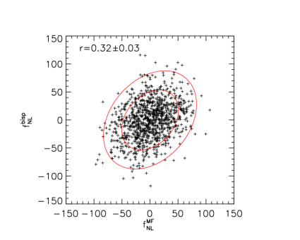
Figure 1: Joint-distribution of $f_{\rm NL}^{\rm MF}$ and $f_{\rm NL}^{\rm bisp}$ from 1000 simulations of the WMAP data including point sources and instrumental noise. We find a correlation coefficient of $r=0.32\pm 0.03$. The $f_{\rm NL}^{\rm MF}$ estimates are obtained from the combination of smoothing the maps at $\theta(\rm FWHM)=10^{\prime},20^{\prime},40^{\prime},80^{\prime},100^{\prime}$. The contours show the 68% and 95% confidence regions of the bivariate Gaussian distribution for $(f_{\rm NL}^{\rm MF},f_{\rm NL}^{\rm bisp})$ with its covariance matrix derived from the simulations.

Using the numerically derived covariance matrix ${\bf C}$, together with our best-fits for $f_{\rm NL}^{\rm MF}$ and $f_{\rm NL}^{\rm bisp}$, we find through Eq. (7) the combined constraint to be

$$\bar{f}_{\rm NL}\equiv f_{\rm NL}^{\rm MF+bisp}=37\pm 28,$$ (8)

which has a $\sim 20\%$ improvement in the error with respect to the individual constraints.

V Conclusions

We evaluated, for the first time, the full covariance matrix for the Minkowski functional estimator of the local-type primordial non-Gaussianity $f_{\rm NL}^{\rm MF}$ and the bispectrum estimator $f_{\rm NL}^{\rm bisp}$. We found the correlation coefficient $r=0.32\pm 0.03$, and used it to combine the constraints from the MF and bispectrum (and their respective variances) to obtain the constraint in Eq. (8). Combining these two estimators hence provides an alternative to improving their “optimality” and leads to combined constraints that are both stronger and more robust. Our work can be extended by using more optimal estimators, e.g. the bispectrum estimator described in Creminelli et al. (2006) whose calculation is numerically very challenging, and by applying to the Planck data, which we leave for future work.

One convenient feature of this work is that, by combining the constraints at the level of MF and bispectrum estimators, we make the problem tractable: an obvious first approach could be to calculate the covariance between the observed bispectrum and MF themselves, but this is extremely complicated, given that the MF and bispectrum are functions of many scales and/or thresholds. Combining the different estimators numerically, as we have done here for the case of local NG, can in principle be rather straightforwardly extended to other types of NG and other cosmological probes. This type of approach is therefore likely to become more widespread with new and better data.

References

- Komatsu (2010) E. Komatsu, Class. Quant. Grav. 27, 124010 (2010).
- Bartolo et al. (2004) N. Bartolo, E. Komatsu, S. Matarrese, and A. Riotto, Phys. Rept. 402, 103 (2004).
- Liguori et al. (2010) M. Liguori, E. Sefusatti, J. Fergusson, and E. Shellard, Adv.Astron. 2010, 980523 (2010).
- Yadav and Wandelt (2010) A. P. Yadav and B. D. Wandelt, Adv.Astron. 2010, 565248 (2010).
- Komatsu and Spergel (2001) E. Komatsu and D. N. Spergel, Phys. Rev. D 63, 063002 (2001).
- Bennett et al. (2012) C. L. Bennett et al., arXiv:1212.5225 (2012).
- Yadav and Wandelt (2008) A. P. Yadav and B. D. Wandelt, Phys.Rev.Lett. 100, 181301 (2008).
- Smith et al. (2009) K. M. Smith, L. Senatore, and M. Zaldarriaga, JCAP 0909, 006 (2009).
- Hikage and Matsubara (2012) C. Hikage and T. Matsubara, Mon. Not. R. Astron. Soc. 425, 2187 (2012).
- Hikage et al. (2006) C. Hikage, E. Komatsu, and T. Matsubara, Astrophys. J. 653, 11 (2006).
- Babich (2005) D. Babich, Phys. Rev. D72, 043003 (2005).
- Creminelli et al. (2006) P. Creminelli, A. Nicolis, L. Senatore, M. Tegmark, and M. Zaldarriaga, JCAP 0605, 004 (2006).
- Ade et al. (2013) P. Ade et al. (Planck Collaboration), arXiv:1303.5084 (2013).
- Creminelli et al. (2007) P. Creminelli, L. Senatore, and M. Zaldarriaga, JCAP 0703, 019 (2007).
- Liguori et al. (2007) M. Liguori, A. Yadav, F. K. Hansen, E. Komatsu, S. Matarrese, et al., Phys.Rev. D76, 105016 (2007).
- Schmalzing and Gorski (1998) J. Schmalzing and K. M. Gorski, Mon. Not. R. Astron. Soc. 297, 355 (1998).
- Tomita (1986) H. Tomita, Progress of Theoretical Physics 76, 952 (1986).
- Matsubara (2003) T. Matsubara, Astrophys. J. 584, 1 (2003).
- Matsubara (2010) T. Matsubara, Phys. Rev. D 81, 083505 (2010).
- Komatsu et al. (2011) E. Komatsu et al., Astrophys. J. Suppl. 192, 18 (2011).
- Komatsu et al. (2009) E. Komatsu et al., Astrophys. J. Suppl. 180, 330 (2009).
- Hikage et al. (2008) C. Hikage et al., Mon. Not. R. Astron. Soc. 389, 1439 (2008).
- Lim and Simon (2012) E. A. Lim and D. Simon, J. Cosmol. Astropart. Phys. 1, 048 (2012).
- Elsner and Wandelt (2009) F. Elsner and B. D. Wandelt, Astrophys. J. Supp. 184, 264 (2009).
- Komatsu et al. (2005) E. Komatsu, D. N. Spergel, and B. D. Wandelt, Astrophys.J. 634, 14 (2005).
- Becker and Huterer (2012) A. Becker and D. Huterer, Phys.Rev.Lett. 109, 121302 (2012).
- Lewis et al. (2000) A. Lewis, A. Challinor, and A. Lasenby, Astrophys.J. 538, 473 (2000).
- Yadav et al. (2008) A. P. S. Yadav, E. Komatsu, B. D. Wandelt, M. Liguori, F. K. Hansen, and S. Matarrese, Astrophys. J. 678, 578 (2008).
- Gorski et al. (2005) K. Gorski, E. Hivon, A. Banday, B. Wandelt, F. Hansen, et al., Astrophys.J. 622, 759 (2005).