Near Minimax Line Spectral Estimation

Abstract

This paper establishes a nearly optimal algorithm for estimating the frequencies and amplitudes of a mixture of sinusoids from noisy equispaced samples. We derive our algorithm by viewing line spectral estimation as a sparse recovery problem with a continuous, infinite dictionary. We show how to compute the estimator via semidefinite programming and provide guarantees on its mean-square error rate. We derive a complementary minimax lower bound on this estimation rate, demonstrating that our approach nearly achieves the best possible estimation error. Furthermore, we establish bounds on how well our estimator localizes the frequencies in the signal, showing that the localization error tends to zero as the number of samples grows. We verify our theoretical results in an array of numerical experiments, demonstrating that the semidefinite programming approach outperforms two classical spectral estimation techniques.

Keywords: Approximate support recovery, Atomic norm, Compressive sensing, Infinite dictionary, Line spectral estimation, Minimax rate, Sparsity, Stable recovery, Superresolution

1 Introduction

Spectrum estimation is one of the fundamental problems in statistical signal processing. Despite of hundreds of years of research on this subject, there still remain several fundamental open questions in this area. This paper addresses a central one of these problems: how well can we determine the locations and magnitudes of spectral lines from noisy temporal samples? In this paper, we establish lower bounds on how well we can recover such signals and demonstrate that these worst case bounds can be nearly saturated by solving a convex programming problem. Moreover, we prove that the estimator approximately localizes the frequencies of the true spectral lines.

We consider signals whose spectra consist of spike trains with unknown locations in a normalized interval $\mathbb{T}=[0,1]$. Consider $n=2m+1$ equispaced samples of a mixture of sinusoids given by

$$x^{\star}_{j}=\sum_{l=1}^{k}c_{l}\exp(i2\pi jf_{l})$$ (1.1)

where $j\in\{-m,\dots,m\}$. We assume that the support $T=\{f_{l}\}_{l=1}^{k}\subset\mathbb{T}$ of the $k$ frequencies and the corresponding complex amplitudes $\{c_{l}\}_{l=1}^{k}$ are unknown. We observe noisy samples $y=x^{\star}+w$ where the noise components $w_{i}$ are i.i.d. centrally symmetric complex Gaussian variables with variance $\sigma^{2}$. By swapping the roles of frequency and time or space, the signal model (1.1) also serves as a proper model for superresolution imaging where we aim to localize temporal events or spatial targets from noisy, low-frequency measurements [1, 2]. Our first result characterizes the denoising error $\frac{1}{n}\lVert x^{\star}-\hat{x}\rVert_{2}^{2}$ and is summarized in the following theorem.

Theorem 1.

Suppose the line spectral signal $x^{\star}$ is given by (1.1) and we observe $n$ noisy consecutive samples $y_{j}=x^{\star}_{j}+w_{j}$ where $w_{j}$ is i.i.d. complex Gaussian with variance $\sigma^{2}$. If the frequencies $\{f_{l}\}_{l=1}^{k}$ in $x^{\star}$ satisfy a minimum separation condition

$$\min_{p\neq q}d(f_{p},f_{q})>4/n$$ (1.2)

with $d(\cdot,\cdot)$ the distance metric on the torus, then we can determine an estimator $\hat{x}$ satisfying

$$\frac{1}{n}\lVert\hat{x}-x^{\star}\rVert_{2}^{2}=O\left(\sigma^{2}\frac{k\log(n)}{n}\right)$$ (1.3)

with high probability by solving a semidefinite programming problem.

Note that if we exactly knew the frequencies $f_{j}$, the best rate of estimation we could achieve would be $O(\sigma^{2}k/n)$ [3]. Our upper bound is merely a logarithmic factor larger than this rate. On the other hand, we will demonstrate via minimax theory that a logarithmic factor is unavoidable when the support is unknown. Hence, our estimator is nearly minimax optimal.

It is instructive to compare our stability rate to the optimal rate achievable for estimating a sparse signal from a finite, discrete dictionary [4]. In the case that there are $p$ incoherent dictionary elements, no method can estimate a $k$-sparse signal from $n$ measurements corrupted by Gaussian noise at a rate less than $O(\sigma^{2}\frac{k\log(p/k)}{n})$. In our problem, there are an infinite number of candidate dictionary elements and it is surprising that we can still achieve such a fast rate of convergence with our highly coherent dictionary. We emphasize that none of the standard techniques from sparse approximation can be immediately generalized to our case. Not only is our dictionary infinite, but also it does not satisfy the usual assumptions such as restricted eigenvalue conditions [5] or coherence conditions [6] that are used to derive stability results in sparse approximation. Nonetheless, in terms of mean-square error performance, our results match those obtained when the frequencies are restricted to lie on a discrete grid.

In the absence of noise, polynomial interpolation can exactly recover a line spectral signal of $k$ arbitrary frequencies with as few as $2k$ equispaced measurements. In the light of our minimum frequency separation requirement (1.2), why should one favor convex techniques for line spectral estimation? Our stability result coupled with minimax optimality establish that no method can perform better than convex methods when the frequencies are well-separated. And, while polynomial interpolation and subspace methods do not impose any resolution limiting assumptions on the constituent frequencies, these methods are empirically highly sensitive to noise. To the best of our knowledge, there is no result similar to Theorem 1 that provides finite sample guarantees about the noise robustness of polynomial interpolation techniques.

Additionally, little is known about how well spectral lines can be localized from noisy observations. The frequencies estimated by any method will never exactly coincide with the true frequencies in the signal in the presence of noise. However, we can characterize the localization performance of our convex programming approach, and summarize this performance in Theorem 2.

Before stating the theorem, we introduce a bit of notation. Define neighborhoods $N_{j}$ around each frequency $f_{j}$ in $x^{\star}$ by $N_{j}:=\{f\in\mathbb{T}:d(f,f_{j})\leq 0.16/n\}$. Also define $F=\mathbb{T}\backslash\cup_{j=1}^{k}N_{j}$ as the set of frequencies in $\mathbb{T}$ which are not near any true frequency. The letters $N$ and $F$ denote the regions that are near to and far from the true supporting frequencies. The following theorem summarizes our localization guarantees.

Theorem 2.

Let $\hat{x}$ be the solution to the same semidefinite programming (SDP) problem as referenced in Theorem 1 and $n>256$. Let $\hat{c_{l}}$ and $\hat{f}_{l}$ form the decomposition of $\hat{x}$ into coefficients and frequencies, as revealed by the SDP. Then, there exist fixed numerical constants $C_{1},C_{2}$ and $C_{3}$ such that with high probability

1. $\sum_{l:\hat{f}_{l}\in F}|\hat{c}_{l}|\leq C_{1}\sigma\sqrt{\frac{k^{2}\log(n)}{n}}$

2. $\sum_{l:\hat{f}_{l}\in N_{j}}|\hat{c}_{l}|\left\{\min_{f_{j}\in T}d(f_{j},\hat{f}_{l})\right\}^{2}\leq C_{2}\sigma\sqrt{\frac{k^{2}\log(n)}{n}}$

3. $\left|c_{j}-\sum_{l:\hat{f_{l}}\in N_{j}}\hat{c}_{l}\right|\leq C_{3}\sigma\sqrt{\frac{k^{2}\log(n)}{n}}$.

4. If for any frequency $f_{j}$, the corresponding amplitude $|c_{j}|>C_{1}\sigma\sqrt{\frac{k^{2}\log(n)}{n}}$, then with high probability there exists a corresponding frequency $\hat{f}_{j}$ in the recovered signal such that,

   $$\left|f_{j}-\hat{f}_{j}\right|\leq\frac{\sqrt{C_{2}/C_{1}}}{n}\left(\frac{|c_{j}|}{C_{1}\sigma\sqrt{\frac{k^{2}\log(n)}{n}}}-1\right)^{-\tfrac{1}{2}}$$

Part (i) of Theorem 2 shows that the estimated amplitudes corresponding to frequencies far from the support are small. In practice, we note that we rarely find any spurious frequencies in the far region, suggesting that our bound (i) is conservative. Parts (ii) and (iii) of the theorem show that in a neighborhood of each true frequency, the recovered signal has amplitude close to the true signal. Part (iv) shows that the larger a particular coefficient is, the better our method is able to estimate the corresponding frequency. In particular, note that if $|c_{j}|>2C_{1}\sigma\sqrt{\frac{k^{2}\log(n)}{n}}$, then $\left|f_{j}-\hat{f}_{j}\right|\leq\frac{\sqrt{C_{2}/C_{1}}}{n}$. In all four parts, note that the localization error goes to zero as the number of samples grows.

We proceed as follows. In Section 2, we begin by contextualizing our result in the canon of line spectral estimation. We emphasize the advantages and shortcomings of prior art, and describe the methods on which our analysis is built upon. We then in Section 3 describe the semidefinite programming approach to line spectral estimation, originally introduced in [7], and explain how it relates to other recent spectrum estimation algorithms. We present minimax lower-bounds for line spectral estimation in Section 4. We then provide the proofs of our main results in Section 5. Finally, in Section 6, we empirically demonstrate that the semidefinite programming approach outperforms MUSIC [8] and Cadzow’s technique [9] in terms of the localization metrics defined by parts (i), (ii) and (iii) of Theorem 2.

2 Prior Art in Line Spectral Estimation

To date, line spectral analysis may be broadly classified into two camps. Subspace methods [8, 10, 9, 11] build upon polynomial interpolation [12] and exploit certain low rank structure in the spectrum estimation problem for denoising. Research on subspace approaches has yielded several standard algorithms that are widely deployed and shown to achieve Cramér-Rao bound asymptotically [13, 14]. However, the sensitivity to noise and model order is not well understood, and there are few guarantees of how these algorithms perform given a limited number of noisy measurements. For a review of many of these classical approaches, see for example [15].

More recently, approaches based on convex optimization have gained favor and have been demonstrated to perform well on a variety of spectrum estimation tasks [16, 17, 18, 19]. These convex programming methods restrict the frequencies to lie on a finite grid of points and view line spectral signals as a sparse combination of single frequencies. While these methods are reported to have significantly better localization properties than subspace methods (see for example, [16]) and admit fast and robust algorithms, they have two significant drawbacks. First, while finer gridding may lead to better performance, very fine grids are often numerically unstable. Furthermore, traditional compressed sensing theory does not adequately characterize the performance of fine gridding in these algorithms as the dictionary becomes highly coherent.

Some very recent work [7, 1, 2] bridges the gap between the performant discretized algorithms and continuous subspace approaches by developing a new theory of convex relaxations for infinite continuous dictionary of frequencies. Our work in [7] applies the atomic norm framework proposed by Chandrasekaran et al [20] to the line spectral estimation problem. There, we established stability results on the denoising error and demonstrated empirically that our algorithm compared favorably with both the classical and recent convex approaches which assume the frequencies are on an oversampled DFT grid. Our prior results made no assumption about the separation between frequencies. When the frequencies are well separated, the current work demonstrates that much faster convergence rates are achieved.

Our work is closely related to recent results established by Candès and Fernandez-Granda [1] on exact recovery using convex methods and their recent work [2] on exploiting the robustness of their dual polynomial construction to show super-resolution properties of convex methods. The total variation norm formulation used in [2] is equivalent to the atomic norm specialized to the line spectral estimation problem.

Robustness bounds were established in both our earlier work [7] and in the work of Candès and Fernandez-Granda [2]. In [7], a slow convergence rate was established with no assumptions about the separation of frequencies in the true signal. In [2], the authors provide guarantees on the $L_{1}$ energy of error in the frequency domain in the case that the frequencies are well separated. The noise is assumed to be adversarial with a small $L_{1}$ spectral energy. In contrast, our paper shows near minimax denoising error under Gaussian noise. It is also not clear that there is a computable formulation for the optimization problem analyzed in [2]. While the guarantees the authors derive in [2] are not comparable with our results, several of their mathematical constructions are used in our proofs here.

Additional recent work derives conditions for approximate support recovery under the Gaussian noise model using the Beurling-Lasso  [21]. There, the authors show that there is a true frequency in the neighborhood of every estimated frequency with large enough amplitude. We note that the Beurling-Lasso is equivalent to the atomic norm algorithm that we analyze in this paper. A more recent paper by Fernandez-Granda[22] improves this result by giving conditions on recoverability in terms of the true signal instead of the estimated signal and prove a theorem similar to Theorem 2, but use a worst case $L_{2}$ bound on the noise samples. Here, we improve these recent results in our proof of Theorem 2, providing tighter guarantees under the Gaussian noise model.

3 Frequency Localization using Atomic Norms

We describe more precisely our signal model in this section. Suppose we wish to estimate the amplitudes and frequencies of a signal $x(t),t\in\mathbb{R}$ given as a mixture of $k$ complex sinusoids:

$$x(t)=\sum_{l=1}^{k}c_{l}\exp(i2\pi f_{l}t)$$

where $\{c_{l}\}_{l=1}^{k}$ are unknown complex amplitudes corresponding to the $k$ unknown frequencies $\{f_{l}\}_{l=1}^{k}$ assumed to be in the torus $\mathbb{T}=[0,1]$. Such a signal may be thought of as a normalized band limited signal and has a Fourier transform given by a line spectrum:

$$\mu(f)=\sum_{l=1}^{k}c_{l}\delta(f-f_{l})$$ (3.1)

Denote by $x^{\star}$ the $n=2m+1$ dimensional vector composed of equispaced Nyquist samples $\{x(j)\}_{j=-m}^{m}$ for $j=-m,\ldots,m$.

The goal of line spectral estimation is to estimate the frequencies and amplitudes of the signal $x(t)$ from the finite, noisy samples $y\in\mathbb{C}^{n}$ given by

$$y_{j}=x_{j}^{\star}+w_{j}\\$$

for $-m\leq j\leq m$, where $w_{j}\sim\mathcal{C}\mathcal{N}(0,\sigma^{2})$ is i.i.d. circularly symmetric complex Gaussian noise.

3.1 Algorithm: Atomic Norm Soft Thresholding (AST)

We can model the line spectral observations $x^{\star}=[x_{-m}^{\star},\ldots,x_{m}^{\star}]^{T}\in\mathbb{C}^{n}$ as a sparse combination of “atoms” $a(f)$ which correspond to observations due to single frequencies. Define the vector $a(f)\in\mathbb{C}^{n}$ for any $f\in\mathbb{T}=[0,1]$ by

$$a(f)=\begin{bmatrix}e^{i2\pi(-m)f}\\ \vdots\\ 1\\ \vdots\\ e^{i2\pi mf}\end{bmatrix}\in\mathbb{C}^{n}.$$

Then, we rewrite model (1.1) as follows:

$$x^{\star}=\sum_{l=1}^{k}c_{l}a(f_{l})=\sum_{l=1}^{k}|c_{l}|a(f_{l})e^{i\phi_{l}}$$ (3.2)

where $\phi_{l}=c_{l}/|c_{l}|$ is the phase of the $l$th component. So, the target signal $x^{\star}$ may be viewed as a sparse non-negative combination of elements from the atomic set $\mathcal{A}$ given by

$$\mathcal{A}=\left\{a(f)e^{i\phi},f\in[0,1],\phi\in[0,2\pi]\right\}.$$ (3.3)

For a general atomic set $\mathcal{A}$, the atomic norm of a vector is defined as the gauge function associated with the convex hull $\operatorname{conv}(\mathcal{A})$ of atoms:

$$\lVert z\rVert_{\mathcal{A}}=\inf\left\{t>0:z\in t\operatorname{conv}(\mathcal{A})\right\}=\inf\left\{\sum_{a}{c_{a}}:z=\sum_{a}{c_{a}a},a\in\mathcal{A},c_{a}>0\right\}$$ (3.4)

The authors in [20] justify the use of atomic norm $\lVert\cdot\rVert_{\mathcal{A}}$ as a general penalty function to promote sparsity in an infinite dictionary $\mathcal{A}$. This generalizes various forms of sparsity. For example, the $\ell^{1}$ norm [23] for sparse vectors is an atomic norm corresponding to the atomic set formed by canonical unit vectors. The nuclear norm [24] for low rank matrices is an atomic norm induced by the atomic set of unit-norm rank-1 matrices.

In this paper, we analyze the performance of the atomic norm soft thresholding (AST) estimate:

$$\hat{x}=\arg\min_{z}\frac{1}{2}\lVert y-z\rVert_{2}^{2}+\tau\lVert z\rVert_{\mathcal{A}}$$ (3.5)

where the atomic norm $\|\cdot\|_{\mathcal{A}}$ corresponds to the atomic set in (3.3), and $\tau$ is a suitably chosen regularization parameter. The corresponding dual problem is interesting because it gives a way of localizing the frequencies in an atomic norm achieving decomposition of $\hat{x}$. The dual problem of AST is given by the following semi-infinite program:

$$\mathop{\operatorname{maximize}}_{q}~{} \frac{1}{2}\lVert y\rVert_{2}^{2}-\frac{1}{2}\lVert y-\tau q\rVert_{2}^{2}$$

subject to $$\sup_{f\in\mathbb{T}}~{}\left|\langle q,a(f)\rangle\right|\leq 1$$ (3.6)

It is convenient to associate a trigonometric polynomial $\hat{Q}(f)=\langle\hat{q},a(f)\rangle$ with the optimal solution $\hat{q}$ of the dual problem. As discussed in [7], the frequencies in the support of the solution $\hat{x}$ can be identified by finding points on the torus $\mathbb{T}$ where $\hat{Q}$ has a magnitude of unity. We use

$$\hat{x}=\sum_{l}\hat{c}_{l}a(\hat{f}_{l})$$ (3.7)

to denote the decomposition of $\hat{x}$ given by the dual polynomial $\hat{Q}(f)$.

We show in [7] that a good choice of $\tau$ for obtaining accelerated convergence rates is

$$\tau=\eta\sigma\sqrt{n\log(n)}$$ (3.8)

for some $\eta\in(1,\infty)$. We shall use this choice of regularization parameter throughout this paper.

Remark.

As shown in Section III.A of our prior work[7], problem (3.5) is equivalent to the semidefinite programming problem

$$\mathop{\operatorname{minimize}}_{z,u,t}~{} \frac{1}{2}\lVert y-z\rVert_{2}^{2}+\frac{\tau}{2}(t+u_{1})$$ (3.9)

$$\operatorname{subject\ to\ } \begin{pmatrix}\operatorname{Toep}(u)&z\\ z^{*}&t\end{pmatrix}\succeq 0.$$ (3.10)

where $\operatorname{Toep}(u)$ denotes a Hermitian Toeplitz matrix with $u$ as its first row and $u_{1}$ is the first component of $u$. Similarly, the dual semi-infinite program (3.1) is equivalent to the dual semidefinite program of (3.9).

4 What is the best rate we can expect?

Using results about minimax achievable rates for linear models  [4, 25], we can deduce that the convergence rate stated in (1.3) is near optimal. Define the set of $k$ well separated frequencies as

$$\mathcal{S}_{k}=\left\{(f_{1},\dots,f_{k})\in\mathbb{T}^{k}~{}\middle|~{}d(f_{p},f_{q})\geq 4/n,p\neq q\right\}$$

The expected minimax denoising error $M_{k}$ for a line spectral signal with frequencies from $\mathcal{S}_{k}$ is defined as the lowest expected denoising error rate for any estimate $\hat{x}(y)$ for the worst case signal $x^{\star}$ with support $T(x^{\star})\in\mathcal{S}_{k}$. Note that we can lower bound $M_{k}$ by restricting the set of candidate frequencies to smaller set. To that end, suppose we restrict the signal $x^{\star}$ to have frequencies only drawn from an equispaced grid on the torus $T_{n}:=\{4j/n\}_{j=1}^{n/4}$. Note that any set of $k$ frequencies from $T_{n}$ are pairwise separated by at least $4/n$. If we denote by $F_{n}$ a $n\times(n/4)$ partial DFT matrix with (unnormalized) columns corresponding to frequencies from $T_{n}$, we can write $x^{\star}=F_{n}c^{\star}$ for some $c^{\star}$ with $\lVert c^{\star}\rVert_{0}=k$. Thus,

$$M_{k} :=\inf_{\hat{x}}\sup_{T(x^{\star})\in\mathcal{S}_{k}}\frac{1}{n}\mathbb{E}\lVert\hat{x}-x^{\star}\rVert_{2}^{2}$$

$$\geq\inf_{\hat{x}}\sup_{\lVert c^{\star}\rVert_{0}\leq k}\frac{1}{n}\mathbb{E}\lVert\hat{x}-F_{n}c^{\star}\rVert_{2}^{2}$$

$$\geq\inf_{\hat{c}}\sup_{\lVert c^{\star}\rVert_{0}\leq k}\frac{1}{n}\mathbb{E}\lVert F_{n}(\hat{c}-c^{\star})\rVert_{2}^{2}$$

$$\geq\frac{n}{4}\left\{\inf_{\hat{c}}\sup_{\lVert c^{\star}\rVert_{0}\leq k}\frac{4}{n}\mathbb{E}\lVert\hat{c}-c^{\star}\rVert_{2}^{2}\right\}\,.$$

Here, the first inequality is the restriction of $T(x^{\star})$. The second inequality follows because we project out all components of $\hat{x}$ that do not lie in the span of $F_{n}$. Such projections can only reduce the Euclidean norm. The third inequality uses the fact that the minimum singular value of $F_{n}$ is $n$ since $F_{n}^{*}F_{n}=nI_{{n}/{4}}$. Now we may directly apply the lower bound for estimation error for linear models derived by Candés and Davenport. Namely, Theorem 1 of [4] states that

$$\inf_{\hat{c}}\sup_{\lVert c^{\star}\rVert_{0}\leq k}\frac{4}{n}\mathbb{E}\lVert\hat{c}-c^{\star}\rVert_{2}^{2} \geq{C}\sigma^{2}\frac{k\log\left(\frac{n}{4k}\right)}{\lVert F_{n}\rVert_{\mathrm{F}}^{2}}\,.$$

With the preceding analysis and the fact that $\lVert F_{n}\rVert_{\mathrm{F}}^{2}=n^{2}/4$, we can thus deduce the following theorem:

Theorem 3.

Let $x^{\star}$ be a line spectral signal as described by (1.1) with the support $T(x^{\star})=\{f_{1},\dots,f_{k}\}\in\mathcal{S}_{k}$ and $y=x^{\star}+w$, where $w\in\mathbb{C}^{n}$ is circularly symmetric Gaussian noise with variance $\sigma^{2}I_{n}$. Let $\hat{x}$ be any estimate of $x^{\star}$ using $y$. Then,

$$M_{k}=\inf_{\hat{x}}\sup_{T(x^{\star})\in\mathcal{S}_{k}}\frac{1}{n}\mathbb{E}\lVert\hat{x}-x^{\star}\rVert_{2}^{2}\geq C\sigma^{2}\frac{k\log\left(\frac{n}{4k}\right)}{n}$$

for some constant $C$ that is independent of $k$, $n$, and $\sigma$.

This theorem and Theorem 1 certify that AST is nearly minimax optimal for spectral estimation of well separated frequencies.

5 Proofs of Main Theorems

In this section, there are many numerical constants. Unless otherwise specified, $C$ will denote a numerical constant whose value may change from equation to equation. Specific constants will be highlighted by accents or subscripts.

We describe the preliminaries and notations, and restate some recent results we used before sketching the proof of Theorems 1 and 2.

5.1 Preliminaries

The sample $x^{\star}_{j}$ may be regarded as the $j$th trigonometric moment of the discrete measure $\mu$ given by (3.1):

$$x_{j}^{\star} = \int_{0}^{1}e^{i2\pi jf}\mu(df)$$

for $-m\leq j\leq m$. Thus, the problem of extracting the frequencies and amplitudes from noisy observations may be regarded as the inverse problem of estimating a measure from noisy trigonometric moments.

We can write the vector $x^{\star}$ of observations $[x_{-m}^{\star},\ldots,x_{m}^{\star}]^{T}$ in terms of an atomic decomposition

$$x^{\star}=\sum_{l=1}^{k}c_{l}a(f_{l})$$

or equivalently in terms of a corresponding representing measure $\mu$ given by (3.1) satisfying

$$x^{\star}=\int_{0}^{1}a(f)\mu(df)$$

There is a one-one correspondence between atomic decompositions and representing measures. Note that there are infinite atomic decompositions of $x^{\star}$ and also infinite corresponding representing measures. However, since every collection of $n$ atoms is linearly independent, $\mathcal{A}$ forms a full spark frame [26] and therefore the problem of finding the sparsest decomposition of $x^{\star}$ is well-posed if there is a decomposition which is at least $n/2$ sparse.

The atomic norm of a vector $z$ defined in (3.4) is the minimum total variation norm [27, 28] $\lVert\mu\rVert_{\mathrm{TV}}$ of all representing measures $\mu$ of $z$. So, minimizing the total variation norm is the same as finding a decomposition that achieves the atomic norm.

5.2 Dual Certificate and Exact Recovery

Atomic norm minimization attempts to recover the sparsest decomposition by finding a decomposition that achieves the atomic norm, i.e., find ${c_{l},f_{l}}$ such that $x^{\star}=\sum_{l}c_{l}a(f_{l})$ and $\lVert x^{\star}\rVert_{\mathcal{A}}=\sum_{l}|c_{l}|$ or equivalently, finding a representing measure $\mu$ of the form (3.1) that minimizes the total variation norm $\lVert\mu\rVert_{\mathrm{TV}}$. The authors of [1] showed that when $n>256$, the decomposition that achieves the atomic norm is the sparsest decomposition by explicitly constructing a dual certificate [29] of optimality, whenever the composing frequencies $f_{1},\ldots,f_{k}$ satisfy a minimum separation condition (1.2). In the rest of the paper, we always make the technical assumption that $n>256$.

Definition 1 (Dual Certificate).

A vector $q\in\mathbb{C}^{n}$ is called a dual certificate for $x^{\star}$ if for the corresponding trigonometric polynomial $Q(f):=\langle q,a(f)\rangle$, we have

$$Q(f_{l})=\operatorname{sign}(c_{l}),l=1,\ldots,k$$

and

$$|Q(f)|<1$$

whenever $f\not\in\{f_{1},\ldots,f_{k}\}$.

The authors of  [1] not only explicitly constructed such a certificate characterized by the dual polynomial $Q$, but also showed that their construction satisfies some stability conditions, which is crucial for showing that denoising using the atomic norm provides stable recovery in the presence of noise.

Theorem 4 (Dual Polynomial Stability, Lemma 2.4 and 2.5 in [2]).

For any $f_{1},\ldots,f_{k}$ satisfying the separation condition (1.2) and any sign vector $v\in\mathbb{C}^{k}$ with $|v_{j}|=1$, there exists a trigonometric polynomial $Q=\left<q,a(f)\right>$ for some $q\in\mathbb{C}^{n}$ with the following properties:

1. For each $j=1,\ldots,k$, $Q$ interpolates the sign vector $v$ so that $Q(f_{j})=v_{j}$

2. In each neighborhood $N_{j}$ corresponding to $f_{j}$ defined by $N_{j}=\left\{f:d(f,f_{j})<{0.16}/{n}\right\}$, the polynomial $Q(f)$ behaves like a quadratic and there exist constants $C_{a},C_{a}^{\prime}$ so that

   $$|Q(f)| \leq 1-\frac{C_{a}}{2}n^{2}(f-f_{j})^{2}$$ (5.1)

   $$|Q(f)-v_{j}| \leq\frac{C_{a}^{\prime}}{2}n^{2}(f-f_{j})^{2}$$ (5.2)

3. When $f\in F=[0,1]\backslash\cup_{j=1}^{k}{N_{j}}$, there is a numerical constant $C_{b}>0$ such that

   $$|Q(f)|\leq 1-C_{b}$$

We use results in [2] and [7] (reproduced in Appendix D for convenience) and borrow several ideas from the proofs in [2], with nontrivial modifications to establish the error rate of atomic norm regularization.

5.3 Proof of Theorem 1

Let $\hat{\mu}$ be the representing measure for the solution $\hat{x}$ of (3.5) with minimum total variation norm, that is,

$$\hat{x}=\int_{0}^{1}a(f)\hat{\mu}(df)$$

and $\lVert\hat{x}\rVert_{\mathcal{A}}=\lVert\hat{\mu}\rVert_{\mathrm{TV}}$. Denote the error vector by $e=x^{\star}-\hat{x}$. Then, the difference measure $\nu=\mu-\hat{\mu}$ is a representing measure for $e$. We first express the denoising error $\lVert e\rVert_{2}^{2}$ as the integral of the error function $E(f)=\langle e,a(f)\rangle,$ against the difference measure $\nu$:

$$\lVert e\rVert_{2}^{2} =\langle e,e\rangle$$

$$=\left\langle e,\int_{0}^{1}a(f)\nu(df)\right\rangle$$

$$=\int_{0}^{1}\left\langle e,a(f)\right\rangle\nu(df)$$

$$=\int_{0}^{1}E(f)\nu(df).$$

Using a Taylor series approximation in each of the near regions $N_{j}$, we first show that the denoising error (or in general any integral of a trigonometric polynomial against the difference measure) can be controlled in terms of an integral in the far region $F$ and the zeroth, first, and second moments of the difference measure in the near regions. The precise result is presented in the following lemma, whose proof is given in Appendix A.

Lemma 1.

Define

$$I_{0}^{j} :=\left|\int_{N_{j}}\nu(df)\right|$$

$$I_{1}^{j} :=n\left|\int_{N_{j}}(f-f_{j})\nu(df)\right|$$

$$I_{2}^{j} :=\frac{n^{2}}{2}\int_{N_{j}}(f-f_{j})^{2}|\nu|(df)$$

$$I_{l} :=\sum_{j=1}^{k}I_{l}^{j},~{}~{}\mbox{for}~{}l=0,1,2\,.$$

Then for any $m$th order trigonometric polynomial $X$, we have

$$\int_{0}^{1}{X(f)\nu(df)}\leq\lVert X(f)\rVert_{\infty}\left(\int_{F}{|\nu|(df)}+I_{0}+I_{1}+I_{2}\right)$$

Applying Lemma 1 to the error function, we get

$$\lVert e\rVert_{2}^{2}\leq\lVert E(f)\rVert_{\infty}\left(\int_{F}{|\nu|(df)}+I_{0}+I_{1}+I_{2}\right)$$ (5.3)

As a consequence of our choice of $\tau$ in (3.8), we can show that $\lVert E(f)\rVert_{\infty}\leq(1+2\eta^{-1})\tau$ with high probability. In fact, we have

$$\lVert E(f)\rVert_{\infty} =\sup_{f\in[0,1]}\left|\langle e,a(f)\rangle\right|$$

$$=\sup_{f\in[0,1]}\left|\langle x^{\star}-\hat{x},a(f)\rangle\right|$$

$$\leq\sup_{f\in[0,1]}\left|\langle w,a(f)\rangle\right|+\sup_{f\in[0,1]}\left|\langle y-\hat{x},a(f)\rangle\right|$$

$$\leq\sup_{f\in[0,1]}\left|\langle w,a(f)\rangle\right|+\tau$$

$$\leq(1+2\eta^{-1})\tau\leq 3\tau,\text{with high probability.}$$ (5.4)

The second inequality follows from the optimality conditions for (3.5). It is shown in Appendix C of  [7] that the penultimate inequality holds with high probability.

Therefore, to complete the proof, it suffices to show that the other terms on the right hand side of (5.3) are $O(\frac{k\tau}{n})$. While there is no exact frequency recovery in the presence of noise, we can hope to get the frequencies approximately right. Hence, we expect that the integral in the far region can be well controlled and the local integrals of the difference measure in the near regions are also small due to cancellations. Next, we utilize the properties of the dual polynomial in Theorems 4 and another polynomial given in Theorem 5 in Appendix B to show that the zeroth and first moments of $\nu$ may be controlled in terms of the other two quantities in (5.3) to upper bound the error rate. The following lemma is similar to Lemmas 2.2 and 2.3 in [2], but we have made several modifications to adapt it to our signal and noise model. For completeness, we provide the proof in Appendix C.

Lemma 2.

There exists numeric constants $C_{0}$ and $C_{1}$ such that

$$I_{0} \leq C_{0}\left(\frac{k\tau}{n}+I_{2}+\int_{F}{|\nu|(df)}\right)$$

$$I_{1} \leq C_{1}\left(\frac{k\tau}{n}+I_{2}+\int_{F}{|\nu|(df)}\right).$$

All that remains to complete the proof is an upper bound on $I_{2}$ and $\int_{F}{|\nu|(df)}$. The key idea in establishing such a bound is deriving upper and lower bounds on the difference $\|P_{T^{c}}(\nu)\|_{{\mathrm{TV}}}-\|P_{T}(\nu)\|_{{\mathrm{TV}}}$ between the total variation norms of $\nu$ on and off the support. The upper bound can be derived using optimality conditions. We lower bound $\|P_{T^{c}}(\nu)\|_{{\mathrm{TV}}}-\|P_{T}(\nu)\|_{{\mathrm{TV}}}$ using the fact that a constructed dual certificate $Q$ has unit magnitude for every element in the support $T$ of $P_{T}(\nu)$ whence we have $\|P_{T}(\nu)\|_{{\mathrm{TV}}}=\int_{\mathbb{T}}Q(f)\nu(df)$. A critical element in deriving both the lower and upper bounds is that the dual polynomial $Q$ has quadratic drop in each near regions $N_{j}$ and is bounded away from one in the far region $F$. Finally, by combing these bounds and carefully controlling the regularization parameter, we get the desired result summarized in the following lemma. The details of the proof are fairly technical and we leave them to Appendix D.

Lemma 3.

Let $\tau=\eta\sigma\sqrt{n\log(n)}$. If $\eta>1$ is large enough, then there exists a numerical constant $C$ such that, with high probability

$$\int_{F}{|\nu|(df)}+I_{2}\leq\frac{Ck\tau}{n}.$$

Putting together Lemmas 1, 2 and 3, we finally prove our main theorem:

$$\frac{1}{n}\lVert e\rVert_{2}^{2} \leq\frac{\lVert E(f)\rVert_{\infty}}{n}\left(\int_{F}{|\nu|(df)}+I_{0}+I_{1}+I_{2}\right)$$

$$\leq\frac{\lVert E(f)\rVert_{\infty}}{n}\left(\frac{C_{1}k\tau}{n}+C_{2}\int_{F}{|\nu|(df)}+C_{3}I_{2}\right)$$

$$\leq\frac{\lVert E(f)\rVert_{\infty}}{n}\frac{Ck\tau}{n}$$

$$\leq\frac{Ck\tau^{2}}{n^{2}}$$

$$=O\left(\sigma^{2}\frac{k\log(n)}{n}\right).$$

The first three inequalities come from successive applications of Lemmas 1, 2 and 3 respectively. The fourth inequality follows from (5.4) and the fifth by our choice of $\tau$ according to Eq. (3.8). This completes the proof of Theorem 1.

5.4 Proof of Theorem 2

The first two statements in Theorem 2 are direct consequences of Lemma 3. For (iii.), we follow [22] and use the dual polynomial $Q_{j}^{\star}(f)=\langle q_{j}^{\star},a(f)\rangle$ constructed in Lemma 2.2 of [22] which satisfies

$$Q_{j}^{\star}(f_{j}) = 1$$

$$|1-Q_{j}^{\star}(f)| \leq n^{2}C_{1}^{\prime}(f-f_{j})^{2},f\in N_{j}$$

$$|Q_{j}^{\star}(f)| \leq n^{2}C_{1}^{\prime}(f-f_{j^{\prime}})^{2},f\in N_{j^{\prime}},j^{\prime}\neq j$$

$$|Q_{j}^{\star}(f)| \leq C_{2}^{\prime},f\in F.$$

We note that $c_{j}-\sum_{\hat{f}_{l}\in N_{j}}\hat{c}_{l}=\int_{N_{j}}\nu(df)$. Then, by applying triangle inequality several times,

$$\left|\int_{N_{j}}\nu(df)\right| \leq\left|\int_{N_{j}}Q_{j}^{\star}(f)\nu(df)\right|+\left|\int_{N_{j}}(1-Q_{j}^{\star}(f))\nu(df)\right|$$

$$\leq\left|\int_{0}^{1}Q_{j}^{\star}(f)\nu(df)\right|+\left|\int_{N_{j}^{c}}Q_{j}^{\star}(f)\nu(df)\right|+\left|\int_{N_{j}}(1-Q_{j}^{\star}(f))\nu(df)\right|$$

$$\leq\left|\int_{0}^{1}Q_{j}^{\star}(f)\nu(df)\right|+\left|\int_{F}Q_{j}^{\star}(f)\nu(df)\right|$$

$$\qquad\qquad\qquad+\sum_{\begin{subarray}{c}j^{\prime}\neq j\\ j^{\prime}=1\end{subarray}}^{k}\int_{N_{j^{\prime}}}\left|Q_{j}^{\star}(f)\right||\nu|(df)+\int_{N_{j}}\left|1-Q_{j}^{\star}(f)\right||\nu(df)|\,.$$

We upper bound the first term using Lemma 5 in Appendix B which yields

$$\left|\int^{0}_{1}Q_{j}^{\star}(f)\nu(df)\right|\leq\frac{Ck\tau}{n}$$

The other terms can be controlled using the properties of $Q_{j}^{\star}$:

$$\left|\int_{F}Q_{j}^{\star}(f)\nu(df)\right| \leq C_{2}^{\prime}\int_{F}|\nu|(df)$$

$$\sum_{\begin{subarray}{c}j^{\prime}\neq j\\ j^{\prime}=1\end{subarray}}^{k}\int_{N_{j^{\prime}}}\left|Q_{j}^{\star}(f)\right||\nu|(df)+\int_{N_{j}}\left|1-Q_{j}^{\star}(f)\right||\nu|(df) \leq C_{1}^{\prime}\sum_{j^{\prime}=1}^{k}\int_{N_{j^{\prime}}}n^{2}(f-f_{j^{\prime}})^{2}|\nu|(df)=C_{1}I_{2}$$

Using Lemma 3, both of the above are upper bounded by $\frac{Ck\tau}{n}$. Now, by combining these upper bounds, we finally have

$$\left|c_{j}-\sum_{l:\hat{f}_{l}\in N_{j}}\hat{c}_{l}\right|\leq\frac{C_{3}k\tau}{n}$$

This shows part (iii) of the theorem. Part (iv) can be obtained by combining parts (ii) and (iii).

6 Experiments

In [7], we demonstrated with extensive experiments that AST outperforms classical subspace algorithms in terms of mean squared estimation error. In the experiments here, we focus on frequency localization and compare the performance of AST, MUSIC [8] and Cadzow’s method [9] under various choices of number of frequencies, number of samples and signal to noise ratios (SNRs).

We adopt the same experimental setup as in [7] and reproduce the description of experiments here for convenience. We generated $k$ normalized frequencies $f_{1},\ldots,f_{k}$ uniformly randomly chosen from $\left[0,1\right]$ such that every pair of frequencies are separated by at least $1/2n$. The signal $x^{\star}\in\mathbb{C}^{n}$ is generated according to (1.1) with $k$ random amplitudes independently chosen from $\chi^{2}(1)$ distribution (squared Gaussian). All of our sinusoids were then assigned a random phase (equivalent to multiplying $c_{l}$ by a random unit norm complex number). The observation $y$ is produced by adding complex white gaussian noise $w$ such that the input signal to noise ratio (SNR) is $-10,-5,0,5,10,15$ or $20$ dB. We compared the average value of the following metrics of the various algorithms in 20 random trials for various values of number of observations $(n=64,128,256)$, and number of frequencies $(k=n/4,n/8,n/16)$.

AST needs an estimate of the noise variance $\sigma^{2}$ to pick the regularization parameter according to (3.8). In our experiments, we do not provide our algorithm with the true noise variance. Instead, we can construct an estimate for $\sigma$ with the following heuristic. We formed the empirical autocorrelation matrix using the MATLAB routine corrmtx using a prediction order $n/3$ and averaging the lower $25\%$ of the eigenvalues. We then use this estimate in equation (3.8) to determine the regularization parameter. See [7] for more details.

We implemented AST using the Alternating Direction Method of Multipliers (ADMM, see for example, [30], or [7] for the specific details). We used the stopping criteria described in [30] and set $\rho=2$ for all experiments. We use the dual solution $\hat{z}$ to determine the support of the optimal solution $\hat{x}$. Once the frequencies $\hat{f}_{l}$ are extracted, we ran the least squares problem $\mbox{minimize}_{\alpha}\|U\alpha-y\|^{2}$ where $U_{jl}=\exp(i2\pi j\hat{f}_{l})$ to obtain debiased estimates of the amplitudes.

We implemented Cadzow’s method as described by the pseudocode in [31], and MUSIC [8] using the MATLAB routine rootmusic. These algorithms need an estimate of the number of sinusoids. Rather than implementing a heuristic to estimate $k$, we fed the true $k$ to our solvers. This provides a significant advantage to these algorithms. On the contrary, AST is not provided the true value of $k$, and the noise variance $\sigma^{2}$ required in the regularization parameter is estimated from $y$.

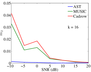
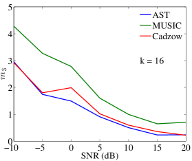
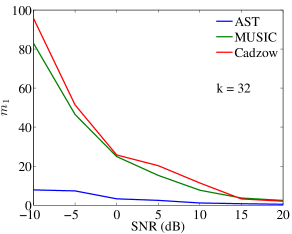
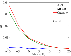
Let $\{\hat{c}_{l}\}$ and $\{\hat{f}_{l}\}$ denote the amplitudes and frequencies estimated by any of the algorithms - AST, MUSIC or Cadzow. We use the following error metrics to characterize the frequency localization of various algorithms:

1. Sum of the absolute value of amplitudes in the far region $F$, $m_{1}=\sum_{l:\hat{f}_{l}\in F}|\hat{c}_{l}|$

2. The weighted frequency localization error, $m_{2}=\sum_{l:\hat{f}_{l}\in N_{j}}|\hat{c}_{l}|\{\min_{f_{j}\in T}d(f_{j},\hat{f}_{l})\}^{2}$

3. Error in approximation of amplitudes in the near region, $m_{3}=\left|c_{j}-\sum_{l:\hat{f_{l}}\in N_{j}}\hat{c}_{l}\right|$

These are precisely the quantities that we prove tend to zero in Theorem 2.

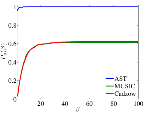
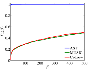
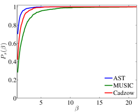
To summarize the results, we first provide performance profiles to summarize the behavior of the various algorithms across all of the parameter settings. Performance profiles provide a good visual indicator of the relative performance of many algorithms under a variety of experimental conditions [32]. Let $\mathcal{P}$ be the set of experiments and let $e_{s}(p)$ be the value of the error measure $e$ of experiment $p\in\mathcal{P}$ using the algorithm $s$. Then the ordinate $P_{s}(\beta)$ of the graph at $\beta$ specifies the fraction of experiments where the ratio of the performance of the algorithm $s$ to the minimum error $e$ across all algorithms for the given experiment is less than $\beta$, i.e.,

$$P_{s}(\beta)=\frac{\mathop{\#}\left\{p\in\mathcal{P}~{}:~{}e_{s}(p)\leq\beta\min_{s}e_{s}(p)\right\}}{\mathop{\#}(\mathcal{P})}$$

(a) $m_{1}$	(b) $m_{2}$	(c) $m_{3}$

Figure 1: Performance Profiles for AST, MUSIC and Cadzow. (a) Sum of the absolute value of amplitudes in the far region ($m_{1}$) (b) The weighted frequency localization error, $m_{2}$ (c) Error in approximation of amplitudes in the near region, $m_{3}$

The performance profiles in Figure 1 show that AST is the best performing algorithm for all the three metrics. AST in fact outperforms MUSIC and Cadzow by a substantial margin for metrics $m_{1}$ and $m_{2}$.

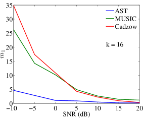
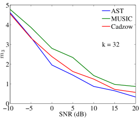
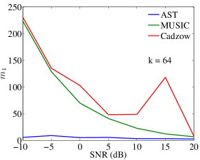
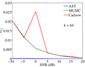
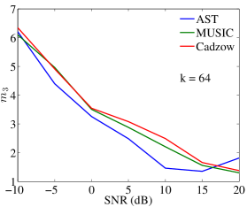
In Figure 2, we display how the error metrics vary with increasing SNR for AST, MUSIC and Cadzow. We restrict these plots to the experiments with $n=256$ samples. These plots demonstrate that AST localizes frequencies substantially better than MUSIC and Cadzow even for low signal to noise ratios as there is very little energy in the far region of the frequencies ($m_{1}$) and has the smallest weighted mean square frequency deviation ($m_{2}$). Although we have plotted the average value in these plots, we observed spikes in the plots for Cadzow’s algorithm as the average is dominated by the worst performing instances. These large errors are due to the numerical instability of polynomial root finding.

Figure 2: For $n=256$ samples, the plots from left to right in order measure the average value over 20 random experiments for the error metrics $m_{1},m_{2}$ and $m_{3}$ respectively. The top, middle and the bottom third of the plots respectively represent the subset of the experiments with the number of frequencies $k=16,32$ and $64$.

7 Conclusion and Future Work

In this paper, we demonstrated stability of atomic norm regularization by analysis of specific properties of the atomic set of moments and the associated dual space of trigonometric polynomials. The key to our analysis is the existence and properties of various trigonometric polynomials associated with signals with well separated frequencies.

Though we have made significant progress at understanding the theoretical limits of line-spectral estimation and superresolution, our bounds could still be improved. For instance, it remains open as to whether the logarithmic term in Theorem 1 can be improved to $\log(n/k)$. Deriving such an upper bound or improving our minimax lower bound would provide an interesting direction for future work.

Additionally, it is not clear if our localization bounds in Theorem 2 have the optimal dependence on the number of sinusoids $k$. For instance, we expect that the condition on signal amplitudes for approximate support recovery should not depend on $k$, by comparison with similar guarantees that have been established for Lasso [33]. We additionally conjecture that for a large enough regularization parameter, there will be no spurious recovered frequencies in the solution. That is, there should be no non-zero coefficients in the “far region” $F$ in Theorem 2. Future work should investigate whether better guarantees on frequency localization are possible.

Appendix A Proof of Lemma 1

We first split the domain of integration into the near and far regions.

$$\left|\int_{0}^{1}X(f)\nu(df)\right| \leq\left|\int_{F}X(f)\nu(f)\right|+\sum_{j=1}^{k}\left|\int_{N_{j}}X(f)\nu(df)\right|$$

$$\leq\lVert X(f)\rVert_{\infty}\int_{F}|\nu|(df)+\sum_{j=1}^{k}\left|\int_{N_{j}}X(f)\nu(df)\right|.$$ (A.1)

by using Hölder’s inequality for the last inequality. Using Taylor’s theorem, we may expand the integrand $X(f)$ around $f_{j}$ as

$$X(f)=X(f_{j})+(f-f_{j})X^{\prime}(f_{j})+\frac{1}{2}X^{\prime\prime}(\xi_{j})(f-f_{j})^{2}$$

for some $\xi_{j}\in N_{j}$. Thus,

$$|X(f)-X(f_{j})-X^{\prime}(f_{j})(f-f_{j})|$$

$$\leq\sup_{\xi\in N_{j}}\frac{1}{2}|X^{\prime\prime}(\xi)|(f-f_{j})^{2}$$

$$\leq\frac{1}{2}n^{2}\lVert X(f)\rVert_{\infty}(f-f_{j})^{2},$$

where for the last inequality we have used a theorem of Bernstein for trigonometric polynomials (see, for example [34]):

$$|X^{\prime}(f_{j})| \leq n\lVert X(f)\rVert_{\infty}$$

$$|X^{\prime\prime}(f_{j})| \leq n^{2}\lVert X(f)\rVert_{\infty}.$$

As a consequence, we have

$$\left|\int_{N_{j}}X(f)\nu(df)\right| \leq\left|X(f_{j})\right|\left|\int_{N_{j}}\nu(df)\right|+\left|X^{\prime}(f_{j})\right|\left|\int_{N_{j}}(f-f_{j})\nu(df)\right|$$

$$+\frac{1}{2}n^{2}\|X(f)\|_{\infty}\int_{N_{j}}(f-f_{j})^{2}|\nu|(df)$$

$$\leq\|X(f)\|_{\infty}\left(I_{0}^{j}+I_{1}^{j}+I_{2}^{j}\right).$$

Substituting back into (A.1) yields the desired result.

Appendix B Some useful lemmas

In addition to Theorem 4, we recall another result in [2] where the authors show the existence of a trigonometric polynomial $Q_{1}$ that is linear in each $N_{j}$ which is also an essential ingredient in our proof.

Theorem 5 (Lemma 2.7 in [2]).

For any $f_{1},\ldots,f_{k}$ satisfying (1.2) and any sign vector $v\in\mathbb{C}^{k}$ with $|v_{j}|=1$, there exists a polynomial $Q_{1}=\left<q_{1},a(f)\right>$ for some $q_{1}\in\mathbb{C}^{n}$ with the following properties:

1. For every $f\in N_{j},$ there exists a numerical constant $C_{a}^{1}$ such that

   $$|Q_{1}(f)-v_{j}(f-f_{j})|\leq\frac{n}{2}C_{a}^{1}(f-f_{j})^{2}$$ (B.1)

2. For $f\in F$, there exists a numerical constant $C_{b}^{1}$ such that

   $$|Q_{1}(f)|\leq\frac{C_{b}^{1}}{n}.$$ (B.2)

We will also need the following straightforward consequence of the constructions of the polynomials in Theorem 4, Theorem 5, and Section 5.4.

Lemma 4.

There exists a numerical constant $C$ such that the constructed $Q(f)$ in Theorem 4, $Q_{1}(f)$ in Theorem 5, and $Q_{j}^{\star}(f)$ in Section 5.4 satisfy respectively

$$\|Q(f)\|_{1} :=\int_{0}^{1}{|Q(f)|df}\leq\frac{Ck}{n}$$ (B.3)

$$\|Q_{1}(f)\|_{1} \leq\frac{Ck}{n^{2}}$$ (B.4)

$$\|Q_{j}^{\star}\|_{1} \leq\frac{Ck}{n}.$$ (B.5)

Proof.

We will give a detailed proof of (B.3), and list the necessary modifications for proving (B.4) and (B.5). The dual polynomial $Q(f)$ constructed in [1] is of the form

$$Q\left(f\right) = \sum_{f_{j}\in T}\alpha_{j}K\left(f-f_{j}\right)+\sum_{f_{j}\in T}\beta_{j}K^{\prime}\left(f-f_{j}\right)$$ (B.6)

where $K\left(f\right)$ is the squared Fejér kernel (recall that $m=(n-1)/2$)

$$K\left(f\right) = \left(\frac{\sin\left(\left(\frac{m}{2}+1\right)\pi f\right)}{\left(\frac{m}{2}+1\right)\sin\left(\pi f\right)}\right)^{4}$$

and for $n\geq 257$, the coefficients $\alpha\in\mathbb{C}^{k}$ and $\beta\in\mathbb{C}^{k}$ satisfy [1, Lemma 2.2]

$$\left\|\alpha\right\|_{\infty} \leq C_{\alpha}$$

$$\left\|\beta\right\|_{\infty} \leq \frac{C_{\beta}}{n}$$

for some numerical constants $C_{\alpha}$ and $C_{\beta}$. Using (B.6) and triangle inequality, we bound $\|Q(f)\|_{1}$ as follows:

$$\|Q(f)\|_{1} = \int_{0}^{1}\left|Q\left(f\right)\right|df$$ (B.7)

$$\leq k\left\|\alpha\right\|_{\infty}\int_{0}^{1}\left|K\left(f\right)\right|df+k\left\|\beta\right\|_{\infty}\int_{0}^{1}\left|K^{\prime}\left(f\right)\right|df$$

$$\leq C_{\alpha}k\int_{0}^{1}\left|K\left(f\right)\right|df+\frac{C_{\beta}}{n}k\int_{0}^{1}\left|K^{\prime}(f)\right|df,$$ (B.8)

To continue, note that $\int_{0}^{1}|K(f)|df=\int_{0}^{1}|G(f)|^{2}df=:\|G(f)\|_{2}^{2}$ where $G(f)$ is the Fejér kernel, since $K(f)$ is the squared Fejér kernel. We can write

$$G(f)=\left(\frac{\sin\left(\pi\left(\frac{m}{2}+1\right)f\right)}{\left(\frac{m}{2}+1\right)\sin(\pi f)}\right)^{2}=\sum_{l=-m/2}^{m/2}g_{l}e^{-i2\pi fl}$$ (B.9)

where $g_{l}=\left(\frac{m}{2}+1-|l|\right)/\left(\frac{m}{2}+1\right)^{2}$. Now, by using Parseval’s identity, we obtain

$$\int_{0}^{1}|K(f)|df = \int_{0}^{1}|G(f)|^{2}df=\sum_{l=-m/2}^{m/2}|g_{l}|^{2}$$ (B.10)

$$= \frac{1}{\left(\frac{m}{2}+1\right)^{4}}\left(\left(\frac{m}{2}+1\right)^{2}+2\sum_{l=1}^{m/2}\left(\frac{m}{2}+1-l\right)^{2}\right)$$

$$= \frac{1}{\left(\frac{m}{2}+1\right)^{4}}\left(\left(\frac{m}{2}+1\right)^{2}+2\sum_{l=1}^{m/2}l^{2}\right)$$

$$\leq \frac{C}{n}$$

for some numerical constant $C$ when $n=2m+1\geq 10$.

Now let us turn our attention to $\int_{0}^{1}|K^{\prime}(f)|df$. Since $K(f)=G(f)^{2}$, we have

$$\int_{0}^{1}|K^{\prime}(f)|df=2\int_{0}^{1}|G(f)G^{\prime}(f)|df\leq 2\|G(f)\|_{2}\|G^{\prime}(f)\|_{2}$$ (B.11)

We have already established that $\|G(f)\|_{2}^{2}\leq C/{n}$ and we will now show that $\|G^{\prime}(f)\|_{2}^{2}\leq C^{\prime}{n}$. Differentiating the expression for $G(f)$ in (B.9), we get

$$G^{\prime}(f) = -2\pi i\sum_{l=-m/2}^{m/2}lg_{l}e^{-i2\pi fl}$$

Therefore, by applying Parseval’s identity again, we get

$$\|G^{\prime}(f)\|_{2}^{2} = 4\pi^{2}\sum_{l=-m/2}^{m/2}l^{2}|g_{l}|^{2}$$

$$\leq \pi^{2}m^{2}\sum_{l=-m/2}^{m/2}|g_{l}|^{2}$$

$$\leq C^{\prime}n$$

Plugging back into (B.11) yields

$$\int_{0}^{1}|K^{\prime}(f)|df\leq C$$ (B.12)

for some constant $C$. Combining (B.12) and (B.10) with (B.8) gives the desired result in (B.3).

The dual polynomial $Q_{1}(f)$ is also of the form (B.6) with coefficient vectors $\alpha_{1}$ and $\beta_{1}$, which satisfy [2, Proof of Lemma 2.7]

$$\|\alpha_{1}\|_{\infty}\leq\frac{C_{\alpha_{1}}}{n},$$

$$\|\beta_{1}\|_{\infty}\leq\frac{C_{\beta_{1}}}{n^{2}}.$$

Combining the above two bounds with (B.7), (B.12) and (B.10) gives the desired result in (B.4).

The last polynomial $Q_{j}^{\star}$ also has the form (B.6) with coefficient vectors $\alpha^{\star}$ and $\beta^{\star}$. According to [22, Proof of Lemma 2.2], these coefficients satisfy

$$\|\alpha^{\star}\|_{\infty}\leq{C_{\alpha_{\star}}},$$

$$\|\beta_{\star}\|_{\infty}\leq\frac{C_{\beta_{\star}}}{n},$$

which yields (B.5) following the same argument leading to (B.3).

∎

Using Lemma 4, we can derive the estimates we need in the following lemma.

Lemma 5.

Let $\nu=\hat{\mu}-\mu$ be the difference measure. Then, there exists numerical constant $C>0$ such that

$$\left|\int_{0}^{1}Q(f)\nu(df)\right| \leq\frac{Ck\tau}{n}$$ (B.13)

$$\left|\int_{0}^{1}Q_{1}(f)\nu(df)\right| \leq\frac{Ck\tau}{n^{2}}$$ (B.14)

$$\left|\int_{0}^{1}Q_{j}^{\star}(f)\nu(df)\right| \leq\frac{Ck\tau}{n}.$$ (B.15)

Proof.

Let $Q_{0}=\langle q_{0},a(f)\rangle$ be a general trigonometric polynomial associated with $q_{0}\in\mathbb{C}^{n}$. Then,

$$\left|\int_{0}^{1}Q_{0}(f)\nu(df)\right| =\left|\int_{0}^{1}\langle q_{0},a(f)\rangle\nu(df)\right|$$

$$=\left|\langle q_{0},\int_{0}^{1}a(f)\nu(df)\rangle\right|$$

$$=\left|\langle q_{0},e\rangle\right|$$

$$=\left|\langle Q_{0}(f),E(f)\rangle\right|$$

$$\leq\lVert Q_{0}(f)\rVert_{1}\lVert E(f)\rVert_{\infty}\,.$$

Here we use Parseval’s identity in the second to last step and Hölder’s inequality in the last inequality. Then, the result follows by using Lemma 4 and (5.4). ∎

We also need the following consequence of the optimality condition of AST from [7, Lemma 2]:

Proposition 1.

$$\tau\lVert\hat{x}\rVert_{\mathcal{A}}\leq\tau\lVert x^{\star}\rVert_{\mathcal{A}}+\langle w,\hat{x}-x^{\star}\rangle$$ (B.16)

Appendix C Proof of Lemma 2

Consider the polar form

$$\int_{N_{j}}\nu(df)=\left|\int_{N_{j}}\nu(df)\right|e^{i\theta_{j}}.$$

Set $v_{j}=e^{-i\theta_{j}}$ and let $Q(f)$ be the dual polynomial promised by Theorem 4 for this $v$. Then, we have

$$\left|\int_{N_{j}}\nu(df)\right| =\int_{N_{j}}e^{-i\theta_{j}}\nu(df)$$

$$=\int_{N_{j}}Q(f)\nu(df)+\int_{N_{j}}(e^{-i\theta_{j}}-Q(f))\nu(df)$$

Summing over $j=1,\ldots,k$ yields

$$I_{0} =\sum_{j=1}^{k}\left|\int_{N_{j}}\nu(df)\right|$$

$$=\sum_{j=1}^{k}\int_{N_{j}}Q(f)\nu(df)+\sum_{j=1}^{k}\int_{N_{j}}(v_{j}-Q(f))\nu(df)$$

$$\leq\left|\int_{0}^{1}Q(f)\nu(df)\right|+\int_{F}|\nu|(df)+C_{a}^{\prime}I_{2},\text{ using triangle inequality and \eqref{q2}}$$

$$\leq\frac{Ck\tau}{n}+\int_{F}|\nu|(df)+C_{a}^{\prime}I_{2},\text{ using \eqref{qv}}.$$ (C.1)

We use a similar argument for bounding $I_{1}$ but this time use the dual polynomial $Q_{1}(f)$ guaranteed by Theorem 5. Again, start with the polar form

$$\int_{N_{j}}(f-f_{j})\nu(df)=\left|\int_{N_{j}}(f-f_{j})\nu(df)\right|e^{i\theta_{j}}=I_{1}^{j}e^{i\theta_{j}}/n$$

Set $v_{j}=e^{-i\theta_{j}}$ in Theorem 5 to obtain

$$I_{1}^{j} =n\int_{N_{j}}e^{-i\theta_{j}}(f-f_{j})\nu(df)$$

$$=n\int_{N_{j}}(v_{j}(f-f_{j})-Q_{1}(f))\nu(df)+n\int_{N_{j}}Q_{1}(f)\nu(df)$$

Summing over $j=1,\ldots,k$ yields

$$I_{1} =\sum_{j=1}^{k}I_{1}^{j}$$

$$=n\sum_{j=1}^{k}\int_{N_{j}}(v_{j}(f-f_{j})-Q_{1}(f))\nu(df)+n\sum_{j=1}^{k}\int_{N_{j}}Q_{1}(f)\nu(df)$$

$$\leq C_{a}^{1}I_{2}+n\left|\int_{0}^{1}Q_{1}(f)\nu(df)\right|+n\left|\int_{F}Q_{1}(f)\nu(df)\right|$$

$$\leq C_{a}^{1}I_{2}+\frac{Ck\tau}{n}+C_{b}^{1}\int_{F}|\nu|(df)$$ (C.2)

For the first inequality, we have used (B.1) and triangle inequality, and for the last inequality, we have used (B.14) and (B.2). Equations (C.1) and (C.2) complete the proof.

Appendix D Proof of Lemma 3

Denote by $P_{T}(\nu)$ the projection of the difference measure $\nu$ on the support set $T=\{f_{1},\ldots,f_{k}\}$ of $x^{\star}$ so that $P_{T}(\nu)$ is supported on $T$. Then, setting $Q(f)$ the polynomial in Theorem 4 that interpolates the sign of $P_{T}(\nu)$, we have

$$\|P_{T}(\nu)\|_{\mathrm{TV}} =\int_{0}^{1}Q(f)P_{T}(\nu)(df)$$

$$\leq\left|\int_{0}^{1}Q(f)\nu(df)\right|+\left|\int_{T^{c}}Q(f)\nu(df)\right|$$

$$\leq\frac{Ck\tau}{n}+\sum_{f_{j}\in T}\left|\int_{N_{j}/\{f_{j}\}}Q(f)\nu(df)\right|+\left|\int_{F}Q(f)\nu(df)\right|,$$

where for the first inequality we used triangle inequality and for the last inequality we used (B.13). The integration over $F$ is can be bounded using Hölder’s inequality

$$\left|\int_{F}Q(f)\nu(df)\right|\leq(1-C_{b})\int_{F}|\nu|(df)$$

We continue with

$$\left|\int_{N_{j}/\{f_{j}\}}Q(f)\nu(df)\right| \leq\left|\int_{N_{j}/\{f_{j}\}}|Q(f)||\nu|(df)\right|$$

$$\leq\int_{N_{j}/\{f_{j}\}}(1-\tfrac{1}{2}n^{2}C_{a}(f-f_{j})^{2})|\nu|(df)$$

$$\leq\int_{N_{j}/\{f_{j}\}}|\nu|(df)-C_{a}I_{2}^{j}.$$

As a consequence, we have

$$\|P_{T}(\nu)\|_{\mathrm{TV}} \leq\frac{Ck\tau}{n}+\sum_{f_{j}\in T}\int_{N_{j}/\{f_{j}\}}|\nu|(df)-C_{a}I_{2}+(1-C_{b})\int_{F}|\nu|(df)$$

$$\leq\frac{Ck\tau}{n}+\underbrace{\sum_{f_{j}\in T}\int_{N_{j}/\{f_{j}\}}|\nu|(df)+\int_{F}|\nu|(df)}_{\|P_{T^{c}}\|_{\mathrm{TV}}}-C_{a}I_{2}-C_{b}\int_{F}|\nu|(df)$$

or equivalently,

$$\|P_{T^{c}}(\nu)\|_{\mathrm{TV}}-\|P_{T}(\nu)\|_{\mathrm{TV}}\geq C_{a}I_{2}+C_{b}\int_{F}|\nu|(df)-\frac{Ck\tau}{n}.$$ (D.1)

Now, we appeal to Proposition 1 and obtain

$$\lVert\hat{x}\rVert_{\mathcal{A}}\leq\lVert x^{\star}\rVert_{\mathcal{A}}-\langle w,e\rangle/\tau$$

and thus

$$\lVert\hat{\mu}\rVert_{\mathrm{TV}}\leq\lVert\mu\rVert_{\mathrm{TV}}+|\langle w,e\rangle|/\tau.$$ (D.2)

Using Lemma 1,

$$|\langle w,e\rangle| =|\langle w,\int_{0}^{1}a(f)\nu(df)|\rangle$$

$$=\left|\int_{0}^{1}\left\langle w,a(f)\right\rangle\nu(df)\right|$$ (D.3)

$$\leq\lVert\left\langle w,a(f)\right\rangle\rVert_{\infty}\left(\frac{Ck\tau}{n}+I_{0}+I_{1}+I_{2}\right)$$

$$\leq 2\eta^{-1}\tau\left(\frac{Ck\tau}{n}+I_{0}+I_{1}+I_{2}\right)$$

$$\leq C\eta^{-1}\tau\left(\frac{k\tau}{n}+I_{2}+\int_{F}|\nu|(df)\right)$$ (D.4)

with high probability, where for the penultimate inequality we used our choice of $\tau$ and $\lVert\left\langle w,a(f)\right\rangle\rVert_{\infty}\leq 2\eta^{-1}\tau$ with high probability, a fact shown in Appendix C of  [7]. Substituting (D) in (D.2), we get

$$\lVert\mu\rVert_{\mathrm{TV}}+C\eta^{-1}\tau\left(\frac{k\tau}{n}+I_{2}+\int_{F}|\nu|(df)\right)$$

$$\geq\lVert\hat{\mu}\rVert_{\mathrm{TV}}$$

$$=\lVert\mu+\nu\rVert_{\mathrm{TV}}$$

$$\geq\lVert\mu\rVert_{\mathrm{TV}}-\lVert{P_{T}(\nu)}\rVert_{\mathrm{TV}}+\lVert{P_{T^{c}}(\nu)}\rVert_{\mathrm{TV}}$$

Canceling $\|\mu\|_{\mathrm{TV}}$ yields

$$\|P_{T^{c}}(\nu)\|_{\mathrm{TV}}-\|P_{T}(\nu)\|_{\mathrm{TV}}\leq C\eta^{-1}\tau\left(\frac{k\tau}{n}+I_{2}+\int_{F}|\nu|(df)\right)$$ (D.5)

As a consequence of (D.1) and (D.5), we get,

$$C(1+\eta^{-1})\frac{k\tau}{n}\geq(C_{b}-\eta^{-1}C)\int_{F}{|\nu|(df)}+(C_{a}-\eta^{-1}C)I_{2}$$

whence the result follows for large enough $\eta.$

References

- [1] E. Candès and C. Fernandez-Granda, “Towards a mathematical theory of super-resolution,” arXiv preprint arXiv:1203.5871, 2012.
- [2] E. Candès and C. Fernandez-Granda, “Super-resolution from noisy data,” arXiv preprint arXiv:1211.0290, 2012.
- [3] F. Bunea, A. Tsybakov, and M. Wegkamp, “Sparsity oracle inequalities for the Lasso,” Electronic Journal of Statistics, vol. 1, pp. 169–194, 2007.
- [4] E. J. Candès and M. A. Davenport, “How well can we estimate a sparse vector?,” Applied and Computational Harmonic Analysis, 2012.
- [5] P. J. Bickel, Y. Ritov, and A. B. Tsybakov, “Simultaneous analysis of lasso and dantzig selector,” The Annals of Statistics, vol. 37, no. 4, pp. 1705–1732, 2009.
- [6] E. J. Candès and Y. Plan, “Near-ideal model selection by minimization,” The Annals of Statistics, vol. 37, no. 5A, pp. 2145–2177, 2009.
- [7] B. N. Bhaskar, G. Tang, and B. Recht, “Atomic norm denoising with applications to line spectral estimation,” arXiv preprint arXiv:1204.0562, 2012.
- [8] R. Schmidt, “Multiple emitter location and signal parameter estimation,” IEEE Trans. on Antennas and Propagation, vol. 34, no. 3, pp. 276–280, 1986.
- [9] J. Cadzow, “Spectral estimation: An overdetermined rational model equation approach,” Proc. of the IEEE, vol. 70, no. 9, pp. 907–939, 1982.
- [10] R. Roy and T. Kailath, “ESPRIT - estimation of signal parameters via rotational invariance techniques,” IEEE Trans. on Acoustics, Speech and Signal Processing, vol. 37, no. 7, pp. 984–995, 1989.
- [11] R. Vautard, P. Yiou, and M. Ghil, “Singular-spectrum analysis: A toolkit for short, noisy chaotic signals,” Physica D: Nonlinear Phenomena, vol. 58, no. 1, pp. 95–126, 1992.
- [12] R. de Prony, “Essai experimental et analytique,” J. Ec. Polytech.(Paris), vol. 2, pp. 24–76, 1795.
- [13] M. Vetterli, P. Marziliano, and T. Blu, “Sampling signals with finite rate of innovation,” IEEE Trans. on Signal Processing, vol. 50, no. 6, pp. 1417–1428, 2002.
- [14] P. Stoica and N. Arye, “MUSIC, maximum likelihood, and Cramér-Rao bound,” IEEE Trans. on Acoustics, Speech and Signal Processing, vol. 37, no. 5, pp. 720–741, 1989.
- [15] P. Stoica and R. Moses, Spectral analysis of signals. Pearson/Prentice Hall, 2005.
- [16] D. Malioutov, M. Çetin, and A. Willsky, “A sparse signal reconstruction perspective for source localization with sensor arrays,” IEEE Trans. on Signal Processing, vol. 53, no. 8, pp. 3010–3022, 2005.
- [17] S. Bourguignon, H. Carfantan, and J. Idier, “A sparsity-based method for the estimation of spectral lines from irregularly sampled data,” IEEE Journal of Selected Topics in Signal Processing, vol. 1, no. 4, pp. 575–585, 2007.
- [18] R. Baraniuk, V. Cevher, M. Duarte, and C. Hegde, “Model-based compressive sensing,” IEEE Trans. on Information Theory, vol. 56, no. 4, pp. 1982–2001, 2010.
- [19] G. Zweig, “Super-resolution fourier transforms by optimisation, and isar imaging,” in IEE Proc. on Radar, Sonar and Navigation, vol. 150, pp. 247–52, IET, 2003.
- [20] V. Chandrasekaran, B. Recht, P. A. Parrilo, and A. S. Willsky, “The convex geometry of linear inverse problems,” Foundations of Computational Mathematics, vol. 12, no. 6, pp. 805–849, 2012.
- [21] J.-M. Azais, Y. De Castro, and F. Gamboa, “Spike detection from inaccurate samplings,” arXiv preprint arXiv:1301.5873, 2013.
- [22] C. Fernandez-Granda, “Support detection in super-resolution,” arXiv preprint arXiv:1302.3921, 2013.
- [23] E. J. Candès, J. Romberg, and T. Tao, “Robust uncertainty principles: exact signal reconstruction from highly incomplete frequency information,” IEEE Trans. Inform. Theory, vol. 52, no. 2, pp. 489–509, 2006.
- [24] E. Candès and B. Recht, “Exact matrix completion via convex optimization,” Foundations of Computational Mathematics, vol. 9, no. 6, pp. 717–772, 2009.
- [25] G. Raskutti, M. J. Wainwright, and B. Yu, “Minimax rates of estimation for high-dimensional linear regression over balls.,” IEEE Transactions on Information Theory, vol. 57, no. 10, pp. 6976–6994, 2011.
- [26] D. L. Donoho and M. Elad, “Optimally sparse representation in general (nonorthogonal) dictionaries via 1 minimization,” Proceedings of the National Academy of Sciences, vol. 100, no. 5, pp. 2197–2202, 2003.
- [27] G. Tang, B. N. Bhaskar, P. Shah, and B. Recht, “Compressed sensing off the grid,” arXiv preprint arXiv:1207.6053, 2012.
- [28] Y. de Castro and F. Gamboa, “Exact reconstruction using Beurling minimal extrapolation,” Journal of Mathematical Analysis and Applications, vol. 395, no. 1, pp. 336 – 354, 2012.
- [29] E. J. Candès and Y. Plan, “A probabilistic and RIPless theory of compressed sensing,” IEEE Trans. on Information Theory, vol. 57, no. 11, pp. 7235–7254, 2011.
- [30] S. Boyd, N. Parikh, B. P. E. Chu, and J. Eckstein, “Distributed optimization and statistical learning via the alternating direction method of multipliers,” Foundations and Trends in Machine Learning, vol. 3, pp. 1–122, December 2011.
- [31] T. Blu, P. Dragotti, M. Vetterli, P. Marziliano, and L. Coulot, “Sparse sampling of signal innovations,” Signal Processing Magazine, IEEE, vol. 25, no. 2, pp. 31–40, 2008.
- [32] E. Dolan and J. Moré, “Benchmarking optimization software with performance profiles,” Mathematical Programming, vol. 91, no. 2, pp. 201–213, 2002.
- [33] E. J. Candès and Y. Plan, “Near-ideal model selection by 1 minimization,” The Annals of Statistics, vol. 37, no. 5A, pp. 2145–2177, 2009.
- [34] A. Schaeffer, “Inequalities of a. markoff and s. bernstein for polynomials and related functions,” Bull. Amer. Math. Soc, vol. 47, pp. 565–579, 1941.