Experimental realisation of quantum illumination

Abstract

We present the first experimental realisation of the quantum illumination protocol proposed in Ref.s [S. Lloyd, Science 321, 1463 (2008); S. Tan et al., Phys. Rev. Lett. 101, 253601 (2008)], achieved in a simple feasible experimental scheme based on photon-number correlations. A main achievement of our result is the demonstration of a strong robustness of the quantum protocol to noise and losses, that challenges some widespread wisdom about quantum technologies.

Properties of quantum states have disclosed the possibility of realizing tasks beyond classical limits, originating a field collectively christened quantum technologies 4 ; 6 ; 7 ; 8 ; 9 ; 10 ; 11 . Among them, quantum metrology and imaging aim to improve the sensitivity and/or resolution of measurements exploiting non-classical features, in particular non classical correlations Kolobov ; Treps:03 ; boy:08 ; bri:10 ; gio:11 . However, in most of the realistic scenarios, losses and noise are known to nullify the advantage of adopting quantum strategies Walmsley-PRL-2011 . Here, we present the first experimental realization of a quantum enhanced scheme llo:08 ; tan:08 , designed to target detection in a noisy environment, preserving a strong advantage over the classical counterparts even in presence of large amount of noise and losses. This work, inspired by theoretical ideas elaborated in llo:08 ; tan:08 ; sha:09 ; gua:09 (see alsoms ), has been implemented exploiting only photon-number correlations in twin beams and, for its accessibility, it can find widespread use. Even more important, it paves the way to real application of quantum technologies by challenging the common believe that they are limited by their fragility to noise and losses.

Our scheme for target detection is inspired by the ”Quantum Illumination” (QI) idea llo:08 ; tan:08 , where the correlation between two beams of a bipartite non-classical state of light is used to detect the target hidden in a noisy thermal background, which is partially reflecting one of the beam. In tan:08 ; sha:09 it was shown that for QI realized by twin beams, like the ones produced by parametric down conversion, there exists in principle an optimal reception strategy offering a significant performance gain respect to any classical strategy. Unfortunately, this quantum optimal receiver, is not yet devised, and even the theoretical proposal of sub-optimal quantum receiver sha:PRA:09 was very challenging from an experimental point of view, and has not been realized yet.

Our aim is to lead the QI idea to an experimental demonstration in a realistic scenario. Therefore, in our realization we consider realistic a-priori unknown background, and a reception strategy based on photon-counting detection and second-order correlation measurements. We demonstrate that the quantum protocol performs astonishingly better than its classical counterpart based on classically-correlated light at any background noise level. More in detail, we compare quantum illumination, specifically twin beams (TWB), with classical illumination (CI) based on correlated thermal beams (THB), that turns out to be the best possible classical strategy in this detection framework.

On the one hand our approach, based on a specific and affordable detection strategy in the context of the current technology, can not aim to achieve the optimal target-detection bounds of Ref. tan:08 , based on quantum Chernoff bound aud:07 ; cal:08 ; pir . On the other hand, it maintains most of the appealing features of the original idea, like a huge quantum enhancement and a robustness against noise, paving the way to future practical application because of the accessible measurement technique. Our study also provides a significant example of ancilla-assisted quantum protocol, besides the few previous realizations, e.g. bri:10 ; bri:ea ; tak ; al .

Figure 1: Experimental setup. a) Quantum illumination: after the BBO crystal, where TWB are generated, one of them (the “ancilla”) is reflected towards the detection system. The correlated beam is partially detected, together with the thermal field from the Arecchi’s disk, when the object (actually a beam splitter) is present, otherwise it is lost (not showed). Low-pass filter (95 % of transmission at 710nm) and UV-reflecting mirror, not showed, are used to minimize the background noise while maintaining low losses. The lens, placed at the focal length from the crystal and the CCD camera, realizes the Fourier transform of the field at the output face of the crystal. b) Classical illumination: one beam from PDC is stopped and the other one is split at a beam splitter (BS) for generating correlated multi-thermal beams. The power of the pump is adjusted to obtain the same energy of the TWB. c) Detected TWB, in the presence of the object, without thermal background. The region of interest is selected by an interference filter centered around the degeneracy wavelength (710 nm) and bandwidth of 10 nm. After selection the filter is removed. d) Detected field for split thermal beams in the presence of the object, without thermal noise. e) A typical frame used for the measurement, where a strong thermal background has been added on the object branch. The colour scales on the right correspond to the number of photons per pixel.

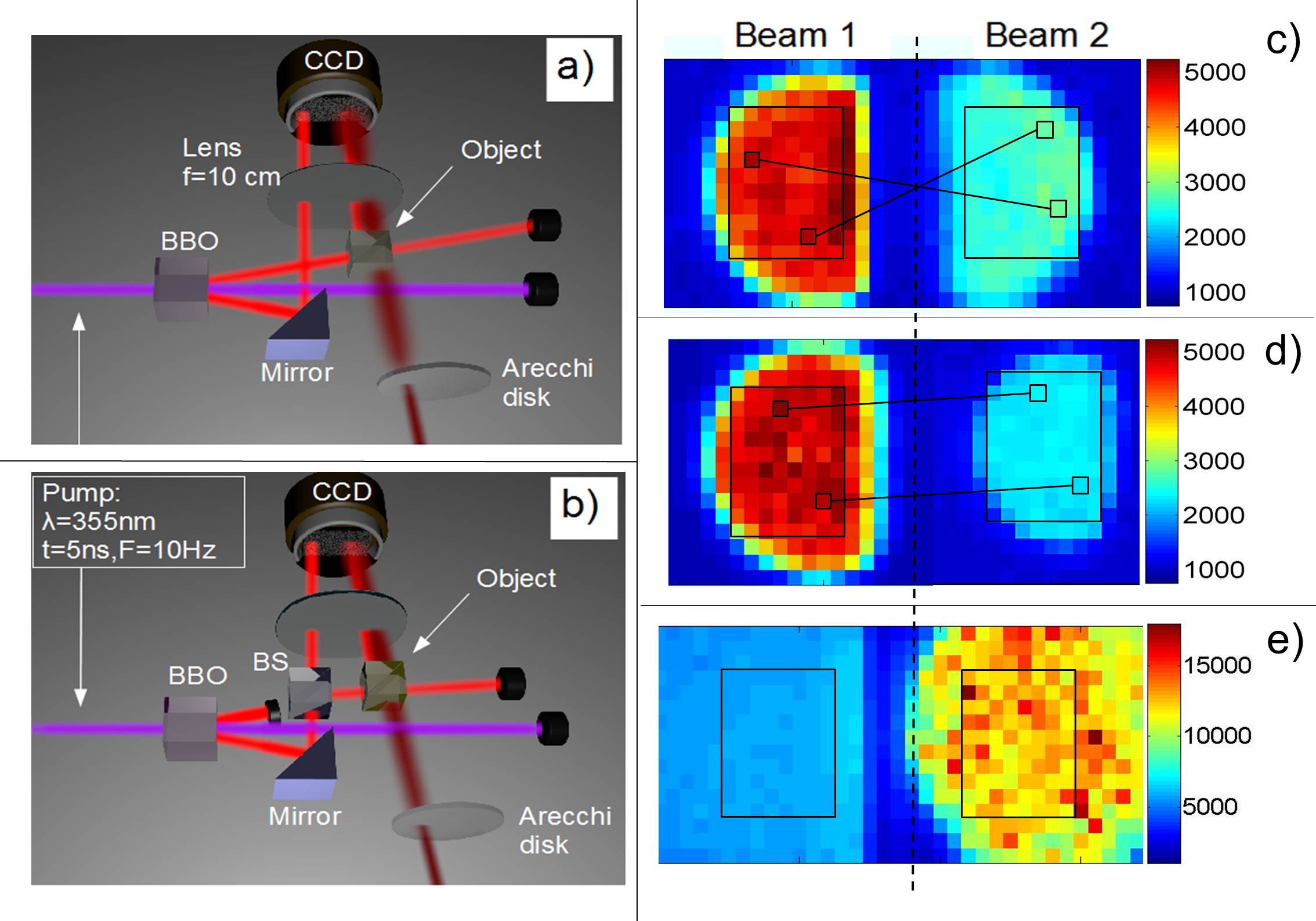
In our set up (see Fig. 1) Parametric Down Conversion (PDC) is exploited to generate two correlated light emissions with average number of PDC photons per spatio-temporal mode $\mu=0.075$, that are then addressed to a high quantum efficiency CCD camera (See Supplementary Information, Sec.I). In the QI protocol (Fig. 1a) one beam is directly detected, while a target object (a 50:50 beam splitter) is posed on the path of the other one, where it is superimposed with a thermal background produced by scattering a laser beam on an Arecchi’s rotating ground glass. When the object is removed, only the background reaches the detector. The CCD camera detects, on different areas, both the optical paths. In the CI protocol (Fig. 1b), the TWB are substituted with classical correlated beams, obtained by splitting a single arm of PDC, that is a multi-thermal beam, and by adjusting the pump intensity to ensure the same intensity, time and spatial coherence properties for the quantum and the classical sources.

We measured the correlation in the photon number $N_{1}$ and $N_{2}$ detected by pairs of pixels intercepting correlated modes of beam ”1” and ”2” respectively (Fig. 1 c-d-e), Brambilla-PRA-2004 ; pra . With our experimental setup, this correlation can be evaluated with a single image by averaging over all the $N_{\rm pix}$ pixels pairs. Albeit the usage of spatial statistic is not strictly necessary, it is practically effective and allows to reduce the measurement time (less images needed)Bri-OptExp:10 .

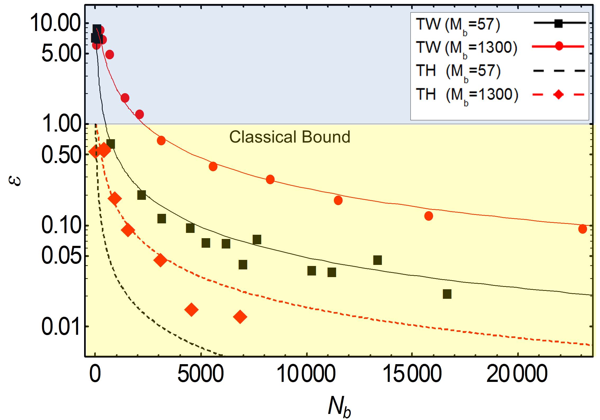
In order to quantify the quantum resources exploited by our QI strategy we introduce a suitable non-classicality parameter: the generalized Cauchy-Schwarz parameter $\varepsilon=\langle:\delta N_{1}\delta N_{2}:\rangle~{}/~{}\sqrt{\langle:\delta^{2}N_{1}:\rangle\langle:\delta^{2}N_{2}:\rangle}$, where $\langle:~{}:\rangle$ is the normally ordered quantum expectation value and $\delta^{2}N_{i}=(N_{i}-\langle N_{i}\rangle)^{2}$ the fluctuation of the photon number $N_{i}$, $i=1,2$. This parameter is interesting since it does not depends on the losses and it quantifies non-classicality: $\varepsilon\leq 1$ for classical state of light (with positive Glauber-Sudarshan $P$-function), while quantum state with negative/singular $P$-function can violate this bound Sekatski2012 . In Fig. 2 we report the measured $\varepsilon$ and the theoretical prediction. One observes that for TWB $\varepsilon^{(QI)}$ is actually in the quantum regime ($\varepsilon^{(QI)}>1$) for small values of the thermal background $\langle N_{b}\rangle$; in absence of it ($\langle N_{b}\rangle=0$) we obtain $\varepsilon^{(QI)}_{0}\simeq 10$. As soon as the contribution of the background to the fluctuation of $N_{2}$ becomes dominant, $\varepsilon^{(QI)}$ decreases quite fast, well below the classical threshold. As expected, for THB $\varepsilon^{(CI)}$ is always in the classical regime, and it is equal to one for $\langle N_{b}\rangle=0$.

Figure 2: Generalized Cauchy-Schwarz parameter $\varepsilon$ in the case of twin beams, $\varepsilon^{(\rm TW)}$, and of the correlated thermal beams, $\varepsilon^{(\rm TH)}$, as a function of the average number of background photons $N_{b}$ for a number of background modes $M_{b}=57$ (black series) and $M_{b}=1300$ (red). The lines represent the theoretical prediction at $\mu=0.075$ (the last estimated independently).

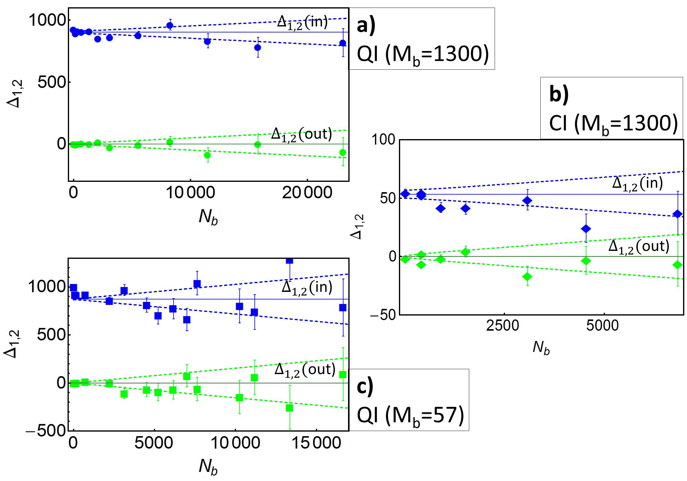
We consider an a-priori unknown background, meaning that it is impossible to establish a reference threshold of photo-counts (usually the mean value of the background) to be compared with the possible additional mean photo-counts coming from the reflected probe beam (if the target is present). Therefore, the estimation of the first order (mean values) of the photo-counts distribution, typical of other protocols (e.g. Treps:03 ; bri:10 ; gio:11 ), is here not informative regarding the presence/absence of the object. We underline that this unknown-background hypothesis accounts for a “realistic” scenario where background properties can randomly change and drift with time and space.

Figure 3: Signal-to-noise ratio (SNR) versus the number of background photons $\langle N_{b}\rangle$ normalized by the square root of number of realization. The red (black) markers refer to $M_{b}=1300$ ($M_{b}=57$) and the solid (dashed) theoretical curve corresponds to quantum (classical) illuminating beams. The estimation of quantum mean values of Eq. (6) is obtained by performing averages of $\Delta_{1,2}^{\rm(in/out)}$ over a set of $N_{\rm img}$ acquired images ($N_{\rm img}=2000,4000,6000$ for twin beams at $M_{b}=1300$, $M_{b}=57$ and thermal beams at $M_{b}=1300$, respectively). The lowest curve of the classical protocol has not been compared with the experimental data because the SNR is so low that a very large number of images (out of the possibility of the actual setup) is required to get reliable points.

Figure 4: Error probability $P_{\rm err}$ of the target detection versus the total number of photons of the thermal background $N_{b}$ evaluated with $N_{\rm img}=10$ ($N_{\rm img}=100$ in the inset). The black squares and red circles are the data for QI with $M_{b}=57$ and $M_{b}=1300$, respectively, while red diamonds referes to the data for the CI with $M_{b}=1300$. The curves are the corresponding theoretical predictions.

For this reason we propose to discriminate the presence/absence of the object by distinguishing between the two corresponding values of the covariance $\Delta_{1,2}$, evaluated experimentally as

$$\Delta_{1,2}=E[N_{1}N_{2}]-E[N_{1}]E[N_{2}].$$ (1)

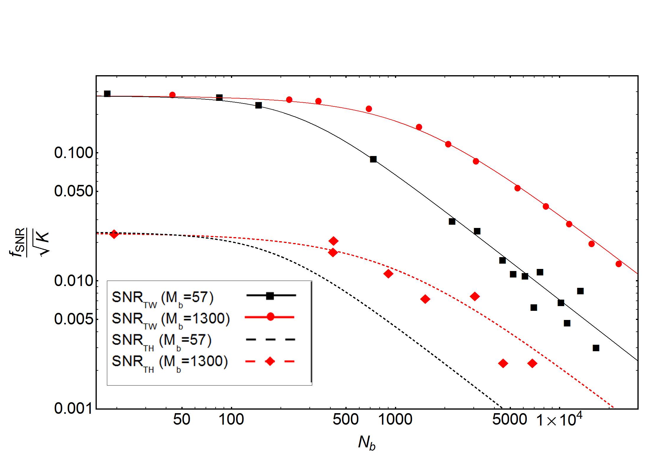
$E[X]=\frac{1}{\mathcal{K}}\sum^{\mathcal{K}}_{k=1}X^{(k)}$ represents the average over the set of $\mathcal{K}$ realizations that in our experiment correspond to the number $\mathcal{K}=N_{\rm pix}$ correlated pixels pairs. The signal-to-noise ratio can be defined as the ratio of the mean “contrast” to its standard deviation (mean fluctuation):

$$f_{\rm SNR}\equiv\frac{\left|\left\langle\Delta_{1,2}^{\rm(in)}-\Delta_{1,2}^{\rm(out)}\right\rangle\right|}{\sqrt{\left\langle\delta^{2}\left(\Delta_{1,2}^{\rm(in)}\right)\right\rangle+\left\langle\delta^{2}\left(\Delta_{1,2}^{\rm(out)}\right)\right\rangle}},$$ (2)

where “in” and “out” refer to the presence and absence of the object.

For $\mathcal{K}>>1$, the “contrast” at the numerator of Eq. (2) corresponds to the quantum expected value of the covariance i.e. $\langle\Delta_{1,2}^{\rm(in)}\rangle\simeq\langle\delta N_{1}\delta N_{2}\rangle$, where obviously $\langle\Delta_{1,2}^{\rm(out)}\rangle=0$. For a generic prominent background with a mean square fluctuation $\langle\delta^{2}N_{b}\rangle$, the “noise” at the denominator depends only on the local statistical properties of the beam 1 and of the uncorrelated background, i.e. $\langle\delta^{2}\Delta_{1,2}\rangle\simeq\langle\delta^{2}N_{1}\rangle\langle\delta^{2}N_{b}\rangle$ (Supplementary Information, Sec.II-a). This is shown in Fig. 5, where the estimated covariance of Eq. (1) is plotted versus the intensity of the thermal background, used in our experiment. As expected, the average value of covariance does not depend on the quantity of environmental noise, while the uncertainty bars do.

While the signal-to-noise ratio unavoidably decreases with the added noise for both QI and CI, the quantum enhancement parameter $(R=f^{(QI)}_{\rm SNR}/f^{(CI)}_{\rm SNR})$ in the presence of dominant background and equal local resources becomes

$$R\approx\langle\delta N_{1}\delta N_{2}\rangle_{QI}/\langle\delta N_{1}\delta N_{2}\rangle_{CI}.$$ (3)

Being $R$ expressed as a ratio of covariances, it is remarkably independent on the amount of losses, noise and reflectivity of the object.

According to Eq. (7) the enhancement is lower bounded by the amount of violation of the Cauchy-Schwarz inequality for the quantum state considered in the absence of background, i.e. $R\simeq\varepsilon^{(QI)}/\varepsilon^{(CI)}\geq\varepsilon^{(QI)}_{0}$. The equality holds for classical states saturating the classical bound, $\varepsilon^{(CI)}_{0}=1$ (Supplementary Information,Sec.B).

In particular, in our experiment we compared the performance of TWB with a classically correlated state with $\varepsilon^{(CI)}_{0}=1$ (hence representing the best possible classical strategy), i.e. with a split thermal beams presenting the same local behaviour of the TWB. In this case the enhancement can be explicitly calculated obtaining $R\simeq(1+\mu)/\mu$, hence the quantum strategy performs orders of magnitude better than the classical analogous when $\mu\ll 1$, namely when a low intensity probe is used.

Incidentally, since covariance is always zero (i.e. $\varepsilon=0$) when using split coherent beams, they do not provide a valuable alternative in the situation considered here, i.e. when first order momenta are not informative due to unknown fluctuating background.

Figure 5: Covariance in the presence, $\Delta_{1,2}^{\rm(in)}$ (blue), or absence, $\Delta_{1,2}^{\rm(out)}$ (green), of the target. a) and b) refer to QI and CI, respectively, for the same number of background modes $M_{b}=1300$; c) refers to QI with a a lower number of modes, $M_{b}=57$. Uncertainty bars represent the effect of the background noise on the covariance estimation (obtained averaging over the $N_{\rm img}=2000,6000$ and $4000$ images in the graphs from the top to bottom, respectively). Horizontal lines are the theoretical values $\langle\Delta_{1,2}^{\rm(in/out)}\rangle$, while the dashed lines are the uncertainty interval evaluated theoretically as $\langle\delta^{2}\Delta_{1,2}^{\rm(in/out)}\rangle/\sqrt{N_{\rm img}}$.

In Fig. 6, the theoretical prediction for $f_{\rm SNR}/\sqrt{\mathcal{K}}$ is compared with the experimental data. In perfect agreement with theory, the quantum enhancement is almost constant ($R\gtrsim 10$) regardless the value of $\langle N_{b}\rangle$. Therefore, the measurement time, i.e. the number of repetitions $N_{\rm img}$ needed for discriminating the presence/absence of the target, is dramatically reduced in QI (for instance, to achieve $f_{\rm SNR}=1$, $N_{\rm img}$ is almost 100 times smaller when quantum correlations are exploited).

Another figure of merit that highlights the superiority of the quantum strategy versus the classical one is the the error probability in the discrimination of the presence/absence of the target ($P_{\mathrm{err}}$). In Fig. 4 we report $P_{\mathrm{err}}$ versus the number of photons of the thermal background $\langle N_{b}\rangle$. $P_{\mathrm{err}}$ is estimated fixing the threshold value of the covariance that minimizes the error probability itself. Fig. 4 shows a remarkable agreement between the theoretical predictions (lines) and the experimental data (symbols), both for QI and CI strategy. $P_{\mathrm{err}}$ of QI is several orders of magnitude below the CI one and, in terms of background photons, the same value of the error probability is reached for a value of $N_{b}$ at least 10 times smaller than in the QI case.

In conclusion, we demonstrated experimentally quantum enhancement in detecting a target in a thermal radiation background. Our system shows quantum correlation ($\varepsilon{(QI)}_{0}\simeq 10$) even in presence of losses introduced by a partially reflective target. Remarkably, even after the transition to the classical regime ($\varepsilon^{(QI)}\ll 1$) due to the presence of background ($\langle N_{b}\rangle\gg 1$), the scheme preserves the same strong advantage with respect to the best classical counterpart based on classically correlated thermal beams. Furthermore, the results are general and do not depend on the specific properties of the background used in the experiment.

In paradigmatic quantum enhanced schemes, often based on the experimental estimation of the first momenta of the photon number distribution, such as quantum imaging protocol bri:10 , detection of small beam displacement Treps:03 and phase estimation by interferometry gio:11 , it is well known that losses and noise rapidly decrease the advantage of using quantum light Walmsley-PRL-2011 . This enforced inside the generic scientific community the common belief that the advantages of entangled and quantum state are hardly applicable in a real context, and they will remain limited to experiments in highly controlled laboratories, and/or to mere academic discussions. Our work breaks this belief showing orders of magnitude improvements compared to CI protocol, independently on the amount of noise and losses using devices available nowadays. In summary, we believe that the photon counting based QI protocol, for its robustness to noise and losses has a huge potentiality to promote the usage of quantum correlated light in real environment.

Acknowledgements

The research leading to these results has received funding from the EU FP7 under grant agreement n. 308803 (BRISQ2), Fondazione SanPaolo and MIUR (FIRB “LiCHIS” - RBFR10YQ3H, Progetto Premiale “Oltre i limiti classici di misura”). SO acknowledges financial support from the University of Trieste (FRA 2009). The authors thank M. G. A. Paris for useful discussions.

I Additional Information on Experimental set-up

In our set up a pump laser beam at 355 nm (triplicated Nd-Yag Q-switched laser) with 5 ns pulses at 10 Hz repetition rate, pumps a type II 7 mm long BBO crystal, cut for producing collinear degenerate emission.

The traveling wave PDC generates a spatially multimode emission, where each mode corresponds to the transverse component of a specific wavevector. Pairs of correlated modes, corresponding to opposite transverse components of the wavevector with respect to the pump direction, are found in symmetric positions in the far field around the degeneracy wavelength of 710 nm[26-28]. Thus, we choose (Fig. 1 c-d-e) two correlated regions of interests on the CCD array, a Princeton Instrument Pixis 400 BRW ($1340X400$ array with pixel size of 20 $\mu$m, high quantum efficiency, more than 80% and low noise in the read out process, about $4$ electrons/pixel). The proper sizing of the pixels and the centering of the 2-dimensional array with sub-mode precision, allows maximizing for each pair of pixels the collection of the correlated photons and at the same time minimizing the possible presence of uncorrelated ones [27,28]. The photon-number-correlation, even at the quantum level for QI, is realized independently for each pairs of symmetrical (translated) pixels belonging to the correlated regions of interests of the TWB (THB). The number of pixel pairs we used is $N_{pix}=80$ with area $A_{\rm pix}=(480\mu\hbox{m})^{2}$. We underline that spatial statistics for the photon-counting-based QI protocol is completely unnecessary. Since QI does not aim an image reconstruction, two conventional photo-counters (i.e. without spatial resolution) will be able to accomplish the evaluation of correlation by temporal statistics, and consequently the QI protocol as well. In our proof-of-principle experiment spatial resolving detectors were employed to have a better control on the statistical properties of the field employed, in order to provide a proper comparison between the experimental data and the theoretical prediction.

The mean number of photons detected per pixel is $\langle N\rangle\simeq 4200$. The number of collected spatio-temporal modes is estimated to be $M=9\cdot 10^{4}$ by fitting a multi-thermal statistics. Thus, taking into account the overall transmission and detection efficiency (about 62% [27]), the average number of PDC photons per mode is $\mu=\langle N\rangle/(\eta M)\simeq 0.075$. We measured separately the size of the spatial mode, as the FWHM of the correlation function between the two beams, $A_{\rm corr}=(120\pm 20\mu\hbox{m})^{2}$. Therefore, the number of spatial modes is about $M_{\rm sp}=A_{\rm pix}/A_{\rm corr}=16\pm 5$ and the number of temporal modes $M_{\rm t}=M/M_{\rm sp}=(6\pm 2)\cdot 10^{3}$, the last one being consistent with the ratio between the pump pulse duration and the expected PDC coherence time, i.e. 1 ps.

The background field is produced by a pulsed laser scattered by a rotating ground glass disk (Arecchi’s disk) and collimating optics. The spatial properties at the CCD plane are set to similar value of the PDC emission, while the temporal modes $M_{b}$ are selected by adjusting the pulse duration and the speed of the disk.

II SNR in case of preponderant background

II.1 Evaluation of $f_{\mathrm{SNR}}$

For a large number of samples $\mathcal{K}>>1$, the “contrast” at the numerator of Eq. (2) of the main text corresponds to the quantum expected value of the covariance, i.e. $\langle\Delta_{1,2}^{\rm(in)}\rangle\simeq\langle\delta N_{1}\delta N_{2}\rangle$, while the mean square fluctuation of the covariance $\langle\delta^{2}\Delta_{1,2}\rangle$ at the denominator can be calculated as

$$\mathcal{K}\left\langle\delta^{2}\Delta_{1,2}\right\rangle\simeq\left\langle\delta^{2}(\delta N_{1}\delta N_{2})\right\rangle\equiv\left\langle\left(\delta N_{1}\delta N_{2}\right)^{2}\right\rangle-\left\langle\delta N_{1}\delta N_{2}\right\rangle^{2}.$$ (4)

By replacing $\delta N_{2}\mapsto\delta N^{(in)}_{2}+\delta N_{b}$ where $N^{(in)}_{2}$ is the number of detected photons that has been reflected by the target, and $N_{b}$ is the uncorrelated background, the right hand side of Eq. (4) can be rewritten as

$$\mathcal{K}\langle\delta^{2}\Delta_{1,2}\rangle \simeq \left\langle\left(\delta N_{1}\delta N^{(in)}_{2}+\delta N_{1}\delta N_{b}\right)^{2}\right\rangle-\left\langle\delta N_{1}\delta N^{(in)}_{2}+\delta N_{1}\delta N_{b}\right\rangle^{2}$$

$$= \left\langle\left(\delta N_{1}\delta N_{2}\right)^{2}\right\rangle-\left\langle\delta N_{1}\delta N_{2}\right\rangle^{2}+\left\langle\delta^{2}N_{1}\right\rangle\left\langle\delta^{2}N_{b}\right\rangle$$

$$= \left\langle\delta^{2}(\delta N_{1}\delta N^{(in)}_{2})\right\rangle+\left\langle\delta^{2}N_{1}\right\rangle\left\langle\delta^{2}N_{b}\right\rangle,$$

where we used the statistical independence of $N_{b}$ and the fact that $\langle\delta N_{b}\rangle=0$. It is clear that in the absence of the target (situation labeled with the superscript ”out”), $N^{(in)}_{2}=0$, thus $\langle\delta^{2}\Delta^{(out)}_{1,2}\rangle=\left\langle\delta^{2}N_{1}\right\rangle\left\langle\delta^{2}N_{b}\right\rangle$, since nothing is reflected to the detector. However, if the the background fluctuations $\left\langle\delta^{2}N_{b}\right\rangle$ is the largest contribution to the noise, also when the target is present (indicated with superscript ”in”) we can write $\langle\delta^{2}\Delta^{(in)}_{1,2}\rangle\simeq\left\langle\delta^{2}N_{1}\right\rangle\left\langle\delta^{2}N_{b}\right\rangle$. Under this assumption representing a realistic situation of a very noisy environment, the SNR becomes

$$f_{\rm SNR}\simeq\frac{\langle\delta N_{1}\delta N_{2}\rangle}{\sqrt{2\left\langle\delta^{2}N_{1}\right\rangle\left\langle\delta^{2}N_{b}\right\rangle}}.$$ (6)

We underline that Eq. (6) holds for a dominant background, irrespective of its statistics (e.g. multi-thermal or Poissonian).

In our experiment we consider background with multi-thermal statistics. For a generic multi-thermal statistics with number of spatiotemporal modes $M$, mean photon number number per mode $\mu$, the total number of detected photons is $\left\langle N\right\rangle=M\eta\mu$ and the mean squared fluctuation is $\left\langle\delta^{2}N\right\rangle=M\eta\mu(1+\eta\mu)=\left\langle N\right\rangle\left(1+\left\langle N\right\rangle/M\right)$ [see for example: L. Mandel, E. Wolf, Optical Coherence and Quantum Optics (Cambridge University Press, 1995)], where $\eta$ is the detection efficiency.

Thus, the amount of noise introduced by the background can be increased by boosting its total number of photons $\left\langle N_{b}\right\rangle$ or by varying the number of modes $M_{b}$, as highlighted from the behaviour of the SNR in Fig.2,3 and 4 of the main text.

Moreover, both TWB and correlated THB present locally the same multi-thermal statistics, but with a number of spatiotemporal modes $M=9\cdot 10^{4}$ much larger than the one used for the background beam ($M_{b}=57$ in one case and, $M_{b}=1.3\cdot 10^{3}$ in the other). This contributes to make the condition of preponderant background effective in our realization, even for a relatively small value of $N_{b}$.

However, we point out that all the theoretical curves reported in all the Figures are evaluated by the exact analytical calculation of the four order (in the number of photons) quantum expectation values appearing on the right hand side of Eq. (4), even if the whole expressions are far more complex than the ones obtained with the assumption of preponderant background.

II.2 Quantum enhancement $R$

Starting from Eq. (6) and considering the same local resources for classical and quantum illumination beams (in particular the same local variance $\left\langle\delta^{2}N_{i}\right\rangle_{CI}=\left\langle\delta^{2}N_{i}\right\rangle_{QI}$ ($i=1,2$)) the enhancement of the quantum protocol can be easily obtained as

$$R=\frac{f^{(QI)}_{\rm SNR}}{f^{(CI)}_{\rm SNR}}\approx\frac{\langle\delta N_{1}\delta N_{2}\rangle_{QI}}{\langle\delta N_{1}\delta N_{2}\rangle_{CI}}=\frac{\varepsilon^{(QI)}}{\varepsilon^{(CI)}}.$$ (7)

with $\varepsilon=\langle:\delta N_{1}\delta N_{2}:\rangle~{}/~{}\sqrt{\langle:\delta^{2}N_{1}:\rangle\langle:\delta^{2}N_{2}:\rangle}$ being the generalized Cauchy-Schwarz parameter introduced in the main text. The covariance of two correlated beams obtained by splitting a single thermal beam is $\langle\delta N_{1}\delta N_{2}\rangle_{TH}=M\eta_{1}\eta_{2}\mu_{TH}^{2}$, while the one of TWB is $\langle\delta N_{1}\delta N_{2}\rangle_{TW}=M\eta_{1}\eta_{2}\mu_{TW}(1+\mu_{TW})$ (see for example Ref. [27]). By using this relation with the assumption of the same local resources, $\mu_{TH}=\mu_{TW}=\mu$ we can derive explicitly $R\approx(1+\mu)/\mu$, which is insensitive to the amount of noise and loss. On the other side the generalized Cauchy-Schwarz parameter for a split thermal beam is $\varepsilon_{0}^{(CI)}=1$, where the subscript ”$0$” stands for ”in absence of background”, as it can be easily derived from the equations of covariance and single beam fluctuations used previously.

As described in the text $\varepsilon_{0}^{(CI)}=1$ represents the best result for classical states and, in this sense, the comparison with split thermal beams represents the comparison with the ”best” classical case.

References

- (1) D. Bouwmeester et al., Nature 390, 575 (1997).
- (2) D. Boschi, S. Branca, F. De Martini, L. Hardy, and S. Popescu, Phys. Rev. Lett. 80, 1121 (1998).
- (3) J. L. O’Brien, Science 318, 1567 (2007).
- (4) X. Yao et al., Nature 482, 489 (2012).
- (5) T. Yamamoto, M. Koashi, S. K. Özdemir, and N. Imoto, Nature 421, 343 (2003).
- (6) J. W. Pan, C. Simon, C. Brukner, and A. Zeilinger, Nature 410, 1067 (2001).
- (7) J. W. Pan, S. Gasparoni, R. Ursin, G. Weihs, and A. Zeilinger, Nature 417, 4174 (2003).
- (8) M. I. Kolobov editor, Quantum Imaging, (Springer, New York, 2007).
- (9) N. Treps et al., Science 301, 940 (2003).
- (10) V. Boyer, A. M. Marino, R. C. Pooser, and P. D. Lett, Science 321, 544 (2008).
- (11) G. Brida, M. Genovese, and I. Ruo Berchera, Nature Photonics 4, 227 (2010).
- (12) V. Giovannetti, S. Lloyd, and L. Maccone, Nat. Phot. 5, 222 (2011).
- (13) N. Thomas-Peter et al., Phys. Rev. Lett. 107, 113603 (2011).
- (14) S. Lloyd, Science 321, 1463 (2008).
- (15) S. Tan et al., Phys. Rev. Lett. 101, 253601 (2008).
- (16) J. H. Shapiro and S. Lloyd, New Journ. of Phys. 11, 063045 (2009).
- (17) S. Guha and B. I. Erkmen, Phys. Rev. A 80, 052310 (2009).
- (18) M. F. Sacchi, Phys. Rev. A 71, 062340 (2005); 72, 014305 (2005).
- (19) J. Shapiro, Phys. Rev. A 80, 022320 (2009).
- (20) K. M. R. Audenaert et al., Phys. Rev. Lett. 98, 160501 (2007).
- (21) J. Calsamiglia, R. Munoz-Tapia, Ll. Masanes, A. Acin, and E. Bagan, Phys. Rev. A 78, 012331 (2008).
- (22) S. Pirandola and S. Lloyd, Phys. Rev. A 77, 032311 (2008).
- (23) G. Brida et al., Phys. Rev. Lett. 108, 253601 (2012)
- (24) H. Takahashi et al., Phys. Rev. Lett. 101, 233605 (2008).
- (25) J. B. Altepeter et al., Phys. Rev. Lett. 90, 193601 (2003).
- (26) E. Brambilla, A. Gatti, M. Bache, and L. A. Lugiato, Phys. Rev. A 69, 023802 (2004).
- (27) G. Brida et al., Opt. Exp. 18, 20572 (2010).
- (28) G. Brida, M. Genovese, A. Meda, and I. Ruo Berchera, Phys. Rev. A 83, 033811 (2011).
- (29) P. Sekatski et al, J. Phys. B 45, 124016 (2012).
- (30) T. Iskhakov, M. V. Chekhova, and G. Leuchs, Phys. Rev. Lett. 102, 183602 (2009).