Discrete flow mapping: transport of phase space densities on triangulated surfaces

Abstract

Energy distributions of high frequency linear wave fields are often modelled in terms of flow or transport equations with ray dynamics given by a Hamiltonian vector field in phase space. Applications arise in underwater and room acoustics, vibro-acoustics, seismology, electromagnetics, and quantum mechanics. Related flow problems based on general conservation laws are used, for example, in weather forecasting or molecular dynamics simulations. Solutions to these flow equations are often large scale, complex and high-dimensional, leading to formidable challenges for numerical approximation methods. This paper presents an efficient and widely applicable method, called discrete flow mapping, for solving such problems on triangulated surfaces. An application in structural dynamics - determining the vibro-acoustic response of a cast aluminium car body component - is presented.

1 Introduction

Wave energy transport in the high frequency limit can be described in terms of the underlying ray dynamics, neglecting interference and other wave effects. The problem is thus reduced to tracking ray densities in phase space and becomes part of a wider class of mass, particle or energy transport problems driven by an underlying deterministic velocity field. Applications are found, for example, in fluid dynamics (Celani et al. (2004)), weather forecasting (Sommer & Reich (2010)), linear wave dynamics or in general in describing the evolution of phase space densities of a dynamical system. The governing equations for the particle or ray densities can often be written in terms of conservation laws (LeVeque (1992)), an example is the Liouville equation describing the evolution of ray densities in phase space for Hamiltonian flows. This class of problems is particularly interesting in the context of approximating linear wave equations in terms of their underlying ray dynamics in the short wavelength limit

Numerical approaches for solving transport problems of this kind are typically based on the method of characteristics, that is, the solutions are found along trajectories or rays determined by the underlying vector field. The flow equations can be formulated in terms of a linear propagator, the so-called Frobenius-Perron (FP) operator (see, for example, Cvitanović et al. (2012)), which describes the evolution of phase space densities in time. Numerically efficient methods for solving flow problems in more than one dimension for a wide class of physically relevant systems are still non-existent. A variety of techniques have been developed based on a FP-operator approach, however, all with a fairly limited range of applicability. Difficulties arise due to the high-dimensionality of the phase space and the singular nature of the operator describing the underlying deterministic dynamics. One approach for dealing with such problems is Ulam’s method (see e.g. Ding & Zhou (1996)), which is based on subdividing the phase space into distinct cells and considering transition rates between these phase space regions. Other methods include wavelet and spectral methods for the infinitesimal FP-operator (Junge & Koltai (2009); Froyland et al. (2013)) and periodic orbit expansion techniques (Lippolis & Cvitanović (2010); Cvitanović et al. (2012)). The modelling of many-particle dynamics, such as protein folding, has been approached using short trajectories of the full, high-dimensional molecular dynamics simulation to construct reduced Markov models (Noé et al. (2009)). For a discussion of convergence properties of the Ulam method in one and several dimensions, see Bose & Murray (2001) and Blank et al. (2002), respectively.

More direct methods are based on tracking swarms of trajectories in phase space often referred to as ray tracing, see for example Červený (2001). Methods related to ray tracing but tracking the time-dynamics of interfaces in phase space, such as moment methods and level set methods, have been developed by Osher & Fedkiw (2001), Engquist & Runborg (2003), Ying & Candès (2006) and Boon et al. (2007) amongst others. They find applications in acoustics, seismology and computer imaging, albeit restricted to problems with few reflections; for an excellent overview, see Runborg (2007). In the following we focus on ray-tracing approximations of linear wave problems, although the methodology developed here can be used in a more general context.

Ray tracing and tracking methods often become inefficient when considering stationary (wave) problems in bounded domains, or in general for ray tracing problems including multiple scattering trajectories and chaotic dynamics. An example is the wave field in a finite cavity driven by a continuous monochromatic excitation. Here, multiple reflections of the rays and complicated folding patterns of the associated level-surfaces often lead to an exponential increase in the number of branches that need to be considered. It is thus necessary to employ approximation methods for the associated ray-tracing solutions, often based on ergodicity and mixing assumptions of the underlying ray dynamics. A popular tool amongst the mechanical engineering community in the context of vibro-acoustic modelling is statistical energy analysis (SEA) (see for example Lyon (1969), Keane (1992) and Lyon & DeJong (1995)). A related method for electromagnetic fields is the random coupling model, which makes use of random field assumptions (see Hemmady et al. (2012)). In SEA the structure is subdivided into a set of subsystems and ergodicity of the underlying ray dynamics as well as quasi-equilibrium conditions are postulated. The result is that the density in each subsystem is taken to be approximately constant leading to greatly simplified equations based only on coupling constants between subsystems. The disadvantage of these methods is that the underlying assumptions are often hard to verify a priori or are only justified when an additional averaging over ‘equivalent’ subsystems is considered. The shortcomings of SEA have been addressed by Langley (1992), Langley & Bercin (1994) and more recently in a series of papers by Le Bot (1998, 2002, 2006).

A computational method called dynamical energy analysis (DEA), which is based on an FP-operator approach, has been introduced by Tanner (2009) and further developed in Chappell et al. (2011). DEA is an Ulam-type method subdividing configuration space into smaller subsystems, but using a basis approximation (spectral method) to obtain an improved resolution of the phase space density. By increasing the resolution in both the position and momentum variable, one systematically interpolates between SEA and full ray tracing thus relaxing the underlying ergodicity and quasi-equilibrium assumptions in SEA. A more computationally efficient approach using a boundary element method for the spatial approximation has been applied to both two and three dimensional problems in Chappell et al. (2012) and Chappell & Tanner (2013). A major advantage of DEA is that by removing the SEA requirements of diffusive wave fields (equivalent to the ergodicity assumption) and quasi-equilibrium conditions, the choice of subsystem division is no longer critical. The resulting increase in flexibility in this choice leads to a much more widely applicable method.

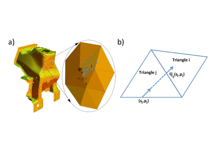
Figure 1: (a) Discrete flow mapping on a mesh of a thin aluminium shell (shock tower) from a Range Rover; (b) the boundary flow map $\varphi_{ij}$ between a pair of adjacent triangles. (Online version in colour.)

In this work, we exploit the freedom in choosing the subsystems by extending DEA towards solving the Liouville equation (or other hyperbolic equations) on meshes. Meshed surfaces are replete in numerical simulation problems thanks largely to the huge popularity of finite element methods. Considering the elements of a mesh as our basic domains therefore automatically renders our techniques applicable to a wide class of problems including the ability to handle complex geometries; an example of which is given in Fig. 1a. A highly efficient solution procedure can be developed for triangulated surfaces since the problem is simplified to considering the local ray dynamics in flat planar regions. In addition, solving phase space flow equations on meshes makes it possible to consider geodesic dynamics on curved surfaces or ray dynamics in non-homogeneous media. This opens up the range of possible applications enormously, for example, in modelling high frequency vibrations of thin elastic shells (see Norris (1995) and Yang et al. (1996)) or in underwater acoustics (Jensen et al. (1993)).

The main outcome of this paper will be the introduction and development of the Discrete Flow Mapping (DFM) technique, a new and efficient method for solving stationary phase space flow equations in complex domains. DFM has similarities to both finite volume methods and boundary integral methods, combining the advantages of each. One achieves the reduction in dimensionality to the boundary of each sub-domain characteristic of boundary integral methods, which in phase space is a reduction by two. In addition one can treat non-homogeneous domains as in finite element and finite volume methods by applying an approximation of local homogeneity and refining the mesh to improve this approximation. A great advantage of DFM is that it can be applied directly to existing finite element models with relatively coarse meshes, and provides a solution for the high frequency case which automatically contains the geometric details absent from SEA-type methods. In addition, the flow directivity can be resolved, unlike in an SEA model, where ergodicity is assumed.

The paper is structured as follows: we will give an integral equation formulation for the stationary Liouville equation on triangulated surfaces in Sec. 2. We then detail the implementation of DFM in Sec. 3; using the linearity of the integral operator, we approximate the solution using a mixture of boundary element and spectral methods. We also discuss the treatment of reflection and transmission on interfaces, such as at edges or due to abrupt changes in material parameters. Finally, in Sec. 4 DFM is applied to model the phase space flow on a sphere and the geodesic flow on an irregularly shaped car body part, demonstrating its power and efficiency in practice.

2 Integral Equation Formulation

We will focus on triangulated surfaces $\Omega=\bigcup_{j=1}^{N_{\Omega}}\Omega_{j}\subset\mathbb{R}^{3}$ consisting of $N_{\Omega}$ triangles $\Omega_{j}$, $j=1,...,N_{\Omega}$ such as depicted in Fig. 1a. We consider piecewise constant Hamiltonians of the form $H_{j}(r,p)=c_{j}|p|=1$ in $\Omega_{j}$ describing the energy of a flow, where $c_{j}$ is the flow velocity for $r\in\Omega_{j}$ and the momentum coordinate $p$ lies on a circle of radius $c_{j}^{-1}$. This Hamiltonian is associated to the Helmholtz equation with inhomogeneous wave velocity $c(r)$ (see Runborg (2007)). In Sec. 3(3.2) we also consider vectorial wave equations, such as plate equations, which include different wave modes. In this case the wave propagation needs to be characterised by more than one Hamiltonian per triangle $j$, that is, we need to consider Hamiltonians $H^{l}_{j}=c_{j}^{l}|p|$, where $l$ refers to the mode type. We restrict our discussion to the scalar case in the following for simplicity of notation.

Let us denote the phase space on the boundary of the triangle $\Omega_{j}$ as $Q_{j}=\partial\Omega_{j}\times(-c_{j}^{-1},c_{j}^{-1})$. The associated coordinates are $X_{j}=(s_{j},p_{j})\in Q_{j}$ with $s_{j}$ parameterising $\partial\Omega_{j}$, the boundary of the $j$th triangle, and $p_{j}\in(-c_{j}^{-1},c_{j}^{-1})$ parameterising the component of the inward momentum (or slowness) vector tangential to $\partial\Omega_{j}$. We denote the boundary flow map as $\varphi_{ij}:Q_{j}\rightarrow Q_{i}$ which takes a vector in $Q_{j}$ and maps it under the flow given through $H_{j}$ to a vector in $Q_{i}$, see Fig. 1b. Note that $\varphi_{ij}$ is generally only defined on a subset of $Q_{j}$, namely the preimage of $Q_{i}$, that is $\varphi_{ij}^{-1}(Q_{i})\subseteq Q_{j}$. This preimage is empty if $\Omega_{j}$ and $\Omega_{i}$ are not adjacent (see Fig. 1).

The stationary density $\rho(X_{i})$ on $Q_{i}$, $i=1,...,N_{\Omega}$, due to an initial boundary distribution $\rho^{(0)}$ on $Q_{j}$, $j=1,...,N_{\Omega}$, may be computed using the following boundary integral equation (see Tanner (2009), Chappell et al. (2012) and Chappell & Tanner (2013)),

$$(I-\mathcal{B})\rho(X_{i})=\rho^{(0)}(X_{i}),$$ (1)

where

$$\mathcal{B}\rho(X_{i}):=\sum_{j}\int_{-c_{j}^{-1}}^{c_{j}^{-1}}\int_{\partial\Omega_{j}}K_{\Gamma}(X_{i},X_{j})\rho(X_{j})ds_{j}dp_{j},$$ (2)

and $K_{\Gamma}$ describes the propagation of the flow. Here we consider purely deterministic flows with $K_{\Gamma}(X_{i},X_{j})=w(X_{i})\,\delta(X_{i}-\varphi_{ij}(X_{j}))$. A diffusion component may be added by replacing the $\delta$-distribution with a finite-width kernel. In general, the weight function $w$ contains reflection/transmission probabilities at boundaries and a dissipative term of the form $\exp(-\mu L)$, where $L$ is the length of the flow trajectory and $\mu$ is a damping coefficient. For the case $w=1$, the transfer operator $\mathcal{B}$ is of Frobenius-Perron type with a maximum eigenvalue one. In this case the problem, Eq. (1), becomes ill-posed and thus we consider the case $\mu>0$ henceforth. One can also obtain a well-posed problem using other forms of dissipation, such as an absorbing or open boundary region (Chappell et al. (2012)). Note that since the flow map only maps to neighbouring triangles, a matrix representation of $\mathcal{B}$ over the whole of $\bigcup_{i=1}^{N_{\Omega}}Q_{i}$ is in general sparse. Equation (1) is a boundary integral formulation for the stationary Liouville equation as detailed in Chappell & Tanner (2013). The derivation of $\rho^{(0)}$ for a high frequency point source is also given in Chappell & Tanner (2013).

3 Implementation of discrete flow mapping

3.1 Discretisation

Typically it is assumed that $\Omega$ consists of a large number of triangles $N_{\Omega}$ describing a geometrically complex domain. A discrete approximation of $\rho$ is sought in phase space coordinates on the triangle boundaries. The spatial approximation is given by taking polynomial basis functions on each triangle edge $\alpha$ with $\alpha=1,2,3$. That is, we split the approximation at corners, see Chappell et al. (2011) for further discussion on the benefits of this choice. In the following, we use piecewise constant functions on the triangle edges for simplicity. In contrast to the position coordinate, the momentum coordinate has support on the interval $(-c_{j}^{-1},c_{j}^{-1})$ only. It is therefore proposed to employ a Legendre polynomial basis approximation in this coordinate (see Chappell et al. (2012)). A key advantage of these choices is that the integrand in the operator (2) remains a very simple function of the position argument and the corresponding integral can be performed analytically. This dramatically reduces the costs of evaluating (2) compared to the implementation used in Chappell et al. (2012).

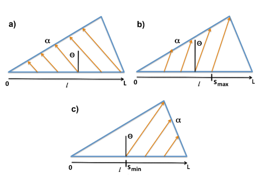
Figure 2: Admissible ranges $(s_{min},s_{max})$ for $s_{j}$ when a ray travels from edge $l$ of triangle $j$ with fixed direction coordinate $p_{j}=\sin(\theta)/c_{j}$ to an opposite edge $\alpha$: (a) $s_{j}$ can take all values in $(0,L)$ on the edge $l$ (i.e. $s_{min}=0$, $s_{max}=L$); (b) $s_{j}\in(0,s_{max})$; (c) $s_{j}\in(s_{min},L)$. (Online version in colour.)

The overall approximation on $Q_{i}$ for $i=1,...,N_{\Omega}$ is then of the form

$$\rho^{\Gamma}(X_{i})\approx\sum_{\alpha=1}^{3}\sum_{\beta=0}^{N_{p}}\rho_{(i,\alpha,\beta)}b_{\alpha}(s_{i})\tilde{P}_{\beta}(p_{i}),$$ (3)

where $N_{p}$ is the order of the momentum basis expansion. The momentum basis functions are given by

$$\tilde{P}_{\beta}(p_{i})={\sqrt{c_{i}}}P_{\beta}(c_{i}p_{i}),$$ (4)

where $P_{\beta}$ is the Legendre polynomial of order $\beta$. The piecewise constant spatial basis functions are given by $b_{\alpha}(s_{i})=2^{-1/2}/\sqrt{A_{\alpha}}$ for $s_{i}$ on the edge $\alpha$, and zero elsewhere. Here $A_{\alpha}$ is the length of the edge $\alpha\in\{1,2,3\}$ of $\Omega_{i}$. Imposing a weak form of the integral equation (1) using the orthonormal inner product for Legendre polynomials $<\cdot,\cdot>$ yields

$$(I-B)\underline{\rho}=\underline{\rho}^{0},$$ (5)

where $I$ is the identity matrix,

$$\rho_{(i,\alpha,\beta)}^{0} = \>\left<\rho^{(0)}(s_{i},p_{i}),b_{\alpha}(s_{i})\tilde{P}_{\beta}(p_{i})\right>,$$ (6)

$$B_{(i,\alpha,\beta),(j,l,m)} = \left<\mathcal{B}\left(b_{l}(s_{i})\tilde{P}_{m}(p_{i})\right),b_{\alpha}(s_{i})\tilde{P}_{\beta}(p_{i})\right>,$$

and the vectors $\underline{\rho}$, $\underline{\rho}^{0}$ have entries given by $\rho_{(i,\alpha,\beta)}$, $\rho_{(i,\alpha,\beta)}^{0}$, respectively. Expanding the inner product in (6) and using the definition of the transfer operator $\mathcal{B}$ (2), the discretised transfer operator $B$ acting on $Q_{i}$ for all $i=1,...,N_{\Omega}$ may be expressed as

$${\displaystyle B_{(i,\alpha,\beta),(j,l,m)}}$$

$${\displaystyle=\frac{2m+1}{4}\int_{Q_{i}}\int_{Q_{j}}\tilde{P}_{\beta}(p_{i})b_{\alpha}(s_{i})K_{\Gamma}(X_{i},X_{j})\tilde{P}_{m}(p_{j})b_{l}(s_{j})ds_{j}dp_{j}ds_{i}dp_{i}}\vspace{2mm}$$

$${\displaystyle=\frac{2m+1}{4}\int_{Q_{j}}w(\psi_{ij}(X_{j}))\tilde{P}_{\beta}(\varphi^{p}_{ij}(X_{j}))b_{\alpha}(\varphi^{s}_{ij}(X_{j}))\tilde{P}_{m}(p_{j})b_{l}(s_{j})ds_{j}dp_{j}.}$$

Here we write $\varphi_{ij}=(\varphi^{s}_{ij},\varphi^{p}_{ij})$ to denote the splitting of the position and momentum parts of the boundary map. Using the properties of the weight function and the spatial basis functions, Eq. (3.1) simplifies to

$$B_{(i,\alpha,\beta),(j,l,m)}=$$ (8)

$$\frac{2m+1}{8\sqrt{A_{\alpha}A_{l}}}\int_{-c_{j}^{-1}}^{c_{j}^{-1}}\tilde{P}_{m}(p_{j})\int_{s_{min}(p_{j},\alpha,l)}^{s_{max}(p_{j},\alpha,l)}w_{rt}(\varphi^{p}_{ij}(X_{j}))e^{-\mu L_{ij}(s_{j},\varphi^{s}_{ij}(X_{j}))}\tilde{P}_{\beta}(\varphi^{p}_{ij}(X_{j}))ds_{j}dp_{j}.$$

Here, $w_{rt}$ is equal to the transmission probability $w_{t}$ when $i\neq j$, and is equal to the reflection probability $w_{r}=1-w_{t}$ otherwise. Higher dimensional transmission/reflection matrices arise in the case of multi-mode dynamics as discussed in the next section. Also $L_{ij}$ is the length of the trajectory from the point represented by $s_{j}$ to $\varphi^{s}_{ij}(X_{j})$, and $(s_{min},s_{max})$ is the admissible range of values for $s_{j}$. Restriction to this range is necessary to ensure that a ray starting on edge $l$ of triangle $j$ with direction coordinate $p_{j}$ will be transferred to a particular adjacent edge $\alpha$ of triangle $i$ as shown in Fig. 2. Note that for flat polygonal elements such as triangles, $\varphi^{p}_{ij}(X_{j})$ in fact only depends on $p_{j}$, and hence only the damping term in equation (8) retains dependence on $s_{j}$. The inner integral thus has a simple form and can be computed analytically, leaving only a single integral to be evaluated numerically. It is this step which leads to vast improvements in the computing times, and enables us to consider many thousands of elements with high order approximations in direction space. Two key points are:

• Triangulation is used to ensure that the elements of a piecewise linear mesh are flat. This enables us to deal with complex enclosures/surfaces whilst keeping the system locally simple.

• Due to the semi-analytic phase space integration, working with many thousands of subsystems and high order direction space approximations becomes tractable.

It is worth pointing out that the analytic integration method is not restricted to triangular elements, but works for any flat polygons. The general idea of the DFM is related to the work in Chappell et al. (2011) and Chappell & Tanner (2013). However, in these papers, the DEA method was developed for general subsystems of arbitrary shape and the double integrals in the equations equivalent to Eq. (8) needed to be computed entirely numerically. Computing the matrix $B$ is then time consuming and the computations were restricted to a small number of subsystems (typically $10$ or less).

3.2 Transmission at interfaces and ray tracing on curved surfaces

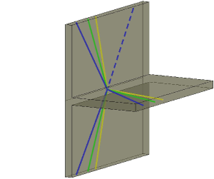
Figure 3: T-joint as an example of a junction between 3 plates. The dashed line indicates an incoming wave, the solid lines represent outgoing bending, shear and pressure waves. (Online version in colour.)

For modelling high frequency wave propagation it will be necessary to take into account transmission (and consequently reflection) at interfaces with abruptly changing material parameters or due to edges and branch lines. The latter will arise, for example, when plates are connected along a common junction such as depicted in Fig. 3. These effects are included in our approach through transmission/reflection probabilities at triangle boundaries coinciding with the interface. The reflection/transmission coefficients are obtained from local wave solutions at the interface, incorporating the dependence on the direction of the incoming and scattered waves. A number of scenarios important in the context of both wave propagation and ray tracing are outlined below.

Scalar wave equations:

For scalar wave equations and simple planar interfaces, the transmission coefficients are derived from the wave equation using continuity of the wave function and its normal derivative for an incident plane wave (see DeSanto (1992)). One thus obtains

$$w_{t}(k_{i},k_{j},\theta_{j})=\frac{4(k_{i}/k_{j})\cos(\theta_{j})\cos(\theta_{i})}{((k_{i}/k_{j})\cos(\theta_{j})+\cos(\theta_{i}))^{2}}.$$ (9)

Here, $k_{j}$ and $k_{i}$ are the wave numbers in the elements containing the incoming and outgoing rays, respectively, with $k_{i}=\omega/c_{i}$ and $\omega$ is the angular frequency. A change of wave vector at the interface may be due to a change in the material parameters for example. The angle of incidence $\theta_{j}$ of the incoming ray with respect to the normal at the element boundary is simply $\arcsin(c_{j}p_{j})$. The direction of the outgoing ray $\theta_{i}$ is determined using Snell’s law.

Elastic waves in coupled plates:

A more general case is represented by interfaces forming junctions between plates of varying thickness and meeting at arbitrary angles. The transmission/reflection coefficients for a set of plates coupled at a common interface (such as depicted in Fig. 3) may be computed using the methods presented in Langley & Heron (1990) and Craik et al. (2004). In particular, we consider the connection between plates as line junctions, that is, the interior properties of the junction are not modelled and the mass and moment of inertia are neglected. Let us consider a line junction which couples $n$ different (for simplicity) semi-infinite plates. The boundary conditions at the line junction correspond to dynamic conditions involving stresses, moments and kinematic conditions for the displacement and rotation of the $n$ plates. To construct the transmission coefficients, we calculate the response of the system with respect to excitation by an incoming plane wave. The incoming wave has a fixed wavenumber and a characteristic mode, that is, it is of bending ($b$), pressure ($p$) or shear ($s$) type. The outgoing waves typically have components in all $n$ plates and are a mixture of all mode types. Evanescent modes may be included to complete the description. Possible material differences between the plates can lead to different wavenumbers in different plates. For a given forcing with a particular incoming mode in a particular plate, we can solve for the unknown modal coefficients in all plates. In practice, we find the transmission probabilities directly by calculating the ratio of outgoing to incoming normal power fluxes. A detailed description can be found in Chappell et al. (2013).

Curved surfaces:

In the case of a geodesic flow on a smooth curved surface it is necessary to mimic the geodesic paths on the corresponding triangulated surface. We employ the theory outlined in Kimmel & Sethian (1998) and Martinez et al. (2005), making use of the fact that for ray paths not intersecting vertices on triangulated surfaces, the notions of shortest and straightest (discrete) geodesic are equivalent (see Martinez et al. (2005)). Hence the straightest geodesic choice of $\theta_{j}=\theta_{i}$ will approximate the direction of the geodesic flow on homogeneous regions of the triangulated surface, and abrupt changes of surface thickness or material will result in a Snell Law effect (see Kimmel & Sethian (1998)). A suitable choice of quadrature method here ensures that the rays never pass through vertices of the triangulation (although a point source may lie on a vertex), for example Gaussian quadrature rules where endpoints are never used as abscissae.

Curved shells - curvature corrections:

For modelling the vibration of thin shells we need to consider ray tracing on curved surfaces, where the dynamics are derived from thin shell theory (Norris (1995)). In a lowest order approximation, curved rays again follow the geodesics of the surface (Yang et al. (1996); Tanner & Søndergaard (2007)). This approximation derives from applying thin shell theory in the high frequency limit as in Norris & Rebinsky (1994) and Norris (1995), which is valid for wavelengths shorter than the radii of curvature of the shell, but larger than the thickness. Corrections to the geodesic ray approximations need to be considered if the local radii of curvature are of the same order as the wavelength. It is possible to construct modified ray paths from the dispersion curves given by thin shell theory (see Norris & Rebinsky (1994)), but this requires a detailed knowledge of the local curvature. In the interests of keeping the model as simple as possible we will follow a different approach here. We treat the meshed structure as a set of plate-like elements and estimate reflection/transmission properties due to the finite angle between mesh elements using the plate-junction theory sketched above and detailed in Langley & Heron (1990) and Craik et al. (2004). This enables us to mimic wave barriers due to regions of high curvature as demonstrated in the next section.

In each of the cases considered above, reflection/transmission coefficients are incorporated as part of the weight function $w$ in the boundary integral kernel $K_{\Gamma}$ in Eq. (2), or its finite dimensional approximation. We assume that the transmission coefficients depend only on the incoming momentum $p_{s}$ via the angle of incidence; the outgoing angle is given by Snell’s law taking into account refraction due to differences in the wave speed across the interface.

4 Numerical examples

We will demonstrate the efficiency and flexibility of DFM with the help of two examples. Firstly, we determine the ray density produced by a point source on a sphere, where an analytic solution is available for verification. Secondly, we compute the energy density distribution on the curved surface of a cast aluminium Range Rover body part and compare with solutions of the corresponding wave equation obtained using the finite element method (FEM).

4.1 Flow on a sphere

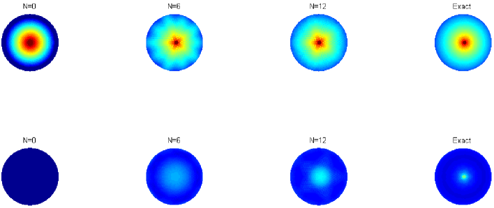
Figure 4: Ray density (logarithmic scale) on a sphere computed using discrete flow mapping showing the source point (upper) and antipode (lower) for different orders of direction space basis ($N_{p}$) on a triangulated sphere with 5120 triangles. The plots on the right show a representation of the exact ray density over the same triangulation. (Online version in colour.)

The ray density $\rho$ generated by a geodesic flow emanating continuously from a point source on a sphere can be determined analytically. As a function of the polar angle $\phi$, with source point $\phi=0$, the ray density is given by:

$$\rho(\phi)=\frac{Ce^{-\mu\phi}}{(1-e^{-2\pi\mu})\sin(\phi)}.$$ (10)

Here, $\mu$ is the damping coefficient introduced in Sec. 2 and $C$ is a constant depending of the strength of the source. The derivation of equation (10) follows simply from the fact that the ray density on the sphere is inversely proportional to the element of surface area. The exponential terms result from damping contributions of the form $\exp(-\mu L)$; summing over the trajectory lengths $L$ at any point on the sphere results in a geometric series with a contribution each time the ray orbits the sphere.

The sphere is thus a good candidate for verifying our approach on an approximately spherical triangulated surface. The dynamics on the sphere are integrable and the exact solution for the density contains a singularity at both poles ($\phi=0$ and $\pi$) as the rays are unidirectional along great circles passing through the source point. This example is therefore slightly atypical since ergodic or mixing ray dynamics in complex geometries generally lead to more smoothly distributed ray densities. The sphere is thus a true challenge for DFM, which due to the finite order basis approximation will always incorporate diffusive behaviour and consequently a smoothing of singularities.

Fig. 4 demonstrates that DFM can deal even with such a singular case. Higher order implementations of the basis approximation in direction space lead to an improved resolution of the refocussed singularity. Table 1 gives the mean relative error averaged over the upper hemisphere containing the source point shown in the upper row of Fig. 4. The results are given for Delaunay triangulations with differing numbers of elements and for different orders of direction space basis. The results are computed at the centroid of each triangle and compared against the exact solution for the same value of $\phi$. For the results presented here we have taken $\mu=1$ and $C=(800\pi^{2})^{-1}$, which is the scaling for a unit excitation of the Helmholtz equation with $k=100\pi$. The factor is derived from the high frequency asymptotics of the 2D fundamental solution for the Helmholtz equation (see Chappell & Tanner (2013)) and matching the asymptotics with equation (10) as the distance from the source becomes small.

Table 1: Mean relative errors computed at triangle centroids and averaged over the upper hemisphere of a Delaunay triangulated sphere with $N_{\Omega}$ triangles and a direction space Legendre polynomial basis approximation of order $N_{p}$.

$N_{\Omega}$	$N_{p}$	Mean Relative Error
320	4	0.1606
320	6	0.1129
320	8	0.1142
1280	8	0.08704
1280	10	0.08884
5120	10	0.06648
5120	12	0.06212
5120	14	0.06100
20480	14	0.05116
20480	16	0.05012

4.2 An Application in Vibro-acoustics

In this section we consider the transport of high frequency flexural or bending wave energy through curved structures using thin shell and high frequency ray models. At present there is wide interest in modelling aluminium shells in the automotive industry due to a desire for lighter, and hence lower emission vehicles. In particular, large molded aluminium components are replacing more traditional multi-component beam-plate constructions, which has the additional advantage of eliminating problems due to fatigue at joints. High frequency vibro-acoustic models based on an SEA treatment will be unsuitable in these circumstances, since complex geometrical features are not included in SEA. In addition, a subdivision of the model into subsystems is not clear cut for such castings as all components are well connected, see for example the structure in Fig. 1a representing an aluminium shock tower from a Range Rover.

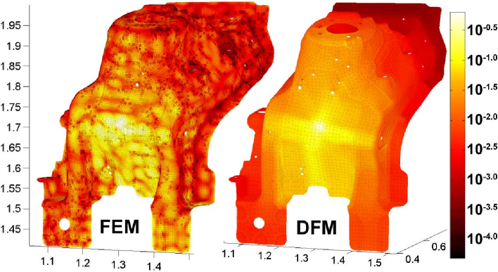
Figure 5: Kinetic energy density on a thin aluminium shell estimated using an averaged full wave finite element model (left) and discrete flow mapping (right) for $3\%$ hysteretic damping. (Online version in colour.)

Discrete flow mapping can overcome these problems, since it can be easily applied in the framework of existing grids for finite element models, requires no choice of subsystem division and incorporates the full geometry and directionality of the energy flow. The response of a thin molded aluminium car component (Range Rover shock tower) to a point force applied normally to the surface is modelled and compared with a FEM approximation for the full wave model performed using Nastran. Figure 1a shows the problem setup including the mesh and indicating the local DFM map $\varphi_{ij}$. In order to maintain a tractable model size for the finite element calculation and to study frequency ranges of industrial interest, the computation is performed at frequencies between 8 kHz and 10 kHz. This approximately corresponds to a third of an octave band centred at 9 kHz. A key assumption of the thin shell theory is that the radius of curvature is large compared to the wavelength (see Norris & Rebinsky (1994)), which is only partly satisfied for this structure in the frequency band considered. The wavelength is typically around $3$ to $6\>$cm depending on the shell thickness. We therefore employ a modified geodesic ray tracing technique by incorporating reflection/transmission due to finite angles between mesh elements as described in Sec. 3(3.2). This leads to geodesic trajectories without reflections in relatively flat areas, but incorporates wave barrier behaviour in regions of high curvature.

Fig. 5 shows the DFM result (bending mode only) compared with the Nastran solution for the kinetic energy averaged over 41 evenly spaced frequencies spanning the prescribed range and with a hysteretic damping level of $3\%$, which is typical for such a structure. The point source is positioned at the front of the structure. The ray computation is performed using a triangulated surface consisting of $11\,623$ triangles and with a 6th order Legendre polynomial basis in direction space. The Nastran grid contains $40\,670$ elements comprising a mix of piecewise linear triangles and quadrilaterals. As would be expected one sees more oscillation in the full wave model. The DFM prediction of the overall energy flow in regions of both high and low curvature matches well with the Nastran results. The flow of energy along the side walls of the central mount, as well as features such as shadow regions due to holes in the structure and channelling effects due to variations in the shell thickness can be observed as common in both plots. Such geometrically dependent features would be entirely absent from SEA-type models and represent a major advance for high frequency vibro-acoustic simulation methods.

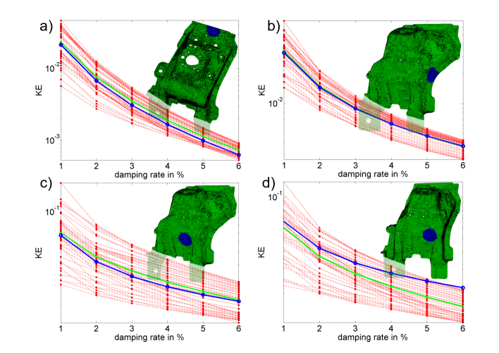
Figure 6: Kinetic energy (KE) response against hysteretic damping level. The KE is averaged over the blue circular receiver regions. DFM: solid blue line with ‘o’ markers; FEM: dotted red lines with ‘$\cdot$’ markers; mean FEM: solid green line with ‘x’ markers. (Online version in colour.)

Figure 6 gives the kinetic energy averaged over four different receiver regions, which are displayed as the blue regions on the inset structure plots. The response is now shown for a range of damping levels between 1$\%$ and 6$\%$, and for receiver regions with differing levels of proximity to the source point. The correspondence between the mean of the 41 Nastran solutions and DFM is remarkably good in Fig.6 (a) to (c). The regions are spread across the whole structure and provide strong verification of our approach. In Fig. 6 (d), the DFM results deviate slightly for high damping. Note that this region is close to the region in Fig. 6 (c) and the deviations thus reflect local variations in the FEM solution. The results clearly demonstrate that curvature related wave-barrier effects are correctly predicted by DFM using local reflection/transmission matrices.

The computations in this section were performed in parallel on four cores of a desktop PC in less than 6 minutes. The code was written in C++ with openMP. The large sparse non-symmetric linear system of dimension 732 249 which arises has been solved efficiently and accurately using a stabilized bi-conjugate gradient iterative solver.

5 CONCLUSIONS

We present discrete flow mapping as a highly efficient method for solving stationary phase space flow equations in complex domains and apply the method to two illustrative examples. In particular we highlight the versatility of the method, its capability to handle large scale models efficiently and emphasise the fact that both geometric details and flow directivity are fully included in the calculation at a moderate computational cost. In the special case of ray focusing, the method clearly captures the foci albeit not reproducing the actual singularity. In the vibro-acoustic example, the full complexity of the model is taken into account via the mesh functionality of DFM. Deviations from a pure geodesic flow due to regions of high curvature have been reproduced without compromising the efficiency of the method. DFM can thus serve as a practical tool for solving phase space transport problems with applications in engineering ranging from acoustics to structural mechanics. Extensions of the method to electrical engineering, as well as to fluid mechanics and other flow problems are evident.

References

- (1)
- Boon et al. (2007) Boon, J.A., Budd, C.J. & Hunt, G.W. (2007) Level set methods for the displacement of layered materials. Proc. R. Soc. A. 463(2082) 1447-1466.
- Bose & Murray (2001) Bose, C.J. & Murray, R. (2001) The exact rate of approximation in Ulam’s method. Discrete and Continuous Dynamical Systems 7 219-235.
- Blank et al. (2002) Blank, M., Keller G. & Liverani C. (2002) Ruelle-Perron-Frobenius spectrum for Anosov maps. Nonlinearity 15 1905-1973.
- Celani et al. (2004) Celani, A., Cencini M., Mazzino A., & Vergassola M. (2004) Active and passive fields face to face, New Journal of Physics 6 72.
- Červený (2001) Červený, V. (2001) Seismic ray theory. (Cambridge University Press, Cambridge, UK).
- Chappell et al. (2011) Chappell, D.J., Giani, S. & Tanner, G. (2011) Dynamical energy analysis for built-up acoustic systems at high frequencies, J. Acoust. Soc. Am. 130(3), 1420-1429.
- Chappell et al. (2012) Chappell, D.J., Tanner, G. & Giani, S. (2012) Boundary element dynamical energy analysis: a versatile high-frequency method suitable for two or three dimensional problems, J. Comp. Phys. 231, 6181-6191.
- Chappell & Tanner (2013) Chappell, D.J. & Tanner, G. (2013) Solving the Liouville Equation via a boundary element method, J. Comp. Phys. 234, 487-498.
- Chappell et al. (2013) Chappell D.J., Löchel D. Søndergaard N. & Tanner, G., (2013) Dynamical energy analysis on mesh grids: a new tool for describing the vibro-acoustic response of engineering structures. To appear in Wave Motion.
- Craik et al. (2004) Craik R. J. M., Bosmans I., Cabos C., Heron K. H., Sarradj E., Steel J. A. & Vermeir G. (2004) Structural transmission at line junctions: a benchmarking exercise, J. Sound Vib. 272, 1086-1096.
- Cvitanović et al. (2012) Cvitanović P., Artuso R. Mainieri R., Tanner G. & and Vattay G. (2012) Chaos: Classical and Quantum, ChaosBook.org (Niels Bohr Institute, Copenhagen, Denmark).
- DeSanto (1992) DeSanto, J.A. (1992) Scalar Wave Theory: Green’s Functions and Applications, (Springer-Verlag, Berlin, Germany) (Chap. 3).
- Ding & Zhou (1996) Ding, J. & Zhou, A. (1996) Finite approximations of Frobenius-Perron operators: A solution of Ulam’s conjecture to multi-dimensional transformations. Physica D 92, 61-68.
- Engquist & Runborg (2003) Engquist, B. & Runborg, O. (2003) Computational high frequency wave propagation. Acta Numerica 12, 181-266.
- Froyland et al. (2013) Froyland, G., Junge, O. & Koltai, P. (2013) Estimating long term behavior of flows without trajectory integration: the infinitesimal generator approach. SIAM J. Num. Anal. 51(1), 223-247.
- Hemmady et al. (2012) Hemmady, S., Antonsen, Jr., T. M., Ott, E., Anlage, S. M. (2012) Statistical Prediction and Measurement of Induced Voltages on Components within Complicated Enclosures: A Wave-Chaotic Approach. IEEE Trans. Electromagnetic Compatibility, 54(4), 758 - 771.
- Jensen et al. (1993) Jensen, F.B., Kuperman, W.J., Porter, M.B. & Schmidt, H. (1993) Computational Ocean Acoustics. (Springer, New York, USA).
- Junge & Koltai (2009) Junge, O. & Koltai, P. (2009) Discretization of the Frobenius-Perron operator using a sparse Haar tensor basis - the Sparse Ulam method. SIAM J. Num. Anal. 47, 3464-3485.
- Keane (1992) Keane, A.J. Energy Flows between Arbitrary Configurations of Conservatively Coupled Multi-Modal Elastic Subsystems. (1992) Proc. R. Soc. Lond. A. 436(1898) 537-568.
- Kimmel & Sethian (1998) Kimmel, R. & Sethian, J.A. (1998) Computing geodesic paths on manifolds. Proceedings of the National Academy of Sciences of the USA 95, 8431-8435.
- Langley & Heron (1990) Langley, R. S. & Heron K. H. (1990) Elastic wave transmission through plate/beam junctions, J. Sound Vib. 143, 241-253.
- Langley (1992) Langley, R.S. (1992) A wave intensity technique for the analysis of high frequency vibrations. J. Sound. Vib. 159, 483-502.
- Langley & Bercin (1994) Langley, R.S. & Bercin, A.N. (1994) Wave intensity analysis for high frequency vibrations. Phil. Trans. Roy. Soc. Lond. A 346, 489-499.
- Le Bot (1998) Le Bot, A. (1998) A vibroacoustic model for high frequency analysis. J. Sound. Vib. 211, 537-554.
- Le Bot (2002) Le Bot, A. (2002) Energy transfer for high frequencies in built-up structures. J. Sound. Vib. 250, 247-275.
- Le Bot (2006) Le Bot, A. (2006) Energy exchange in uncorrelated ray fields of vibroacoustics. J. Acoust. Soc. Am. 120(3), 1194-1208.
- LeVeque (1992) LeVeque, R. J. (1992) Numerical Methods for Conservation Laws. Lectures in Mathematics: ETH Zürich, (Birkhäuser, Basel, Swizerland).
- Lippolis & Cvitanović (2010) Lippolis, D. & Cvitanović, P. (2010) How well can one resolve the state space of a chaotic map? Phys. Rev. Lett., 104, 014101.
- Lyon (1969) Lyon, R.H. (1969) Statistical analysis of power injection and response in structures and rooms. J. Acoust. Soc. Am. 45, 545-565.
- Lyon & DeJong (1995) Lyon R.H. & DeJong R. G. (1995) Theory and Application of Statistical Energy Analysis, (Butterworth-Heinemann, Boston, USA), 2nd edn.
- Martinez et al. (2005) Martinez, D., Vehlo, L. & Carvalho, P.C. (2005) Computing geodesics on triangular meshes. Computers & Graphics 29, 667-675.
- Noé et al. (2009) Noé F., Schütte C., Vanden-Eijnden E., Reich L. & Weikl T. R. (2009) Constructing the equilibrium ensemble of folding pathways from short off-equilibrium simulations. Proceedings of the National Academy of Sciences of the USA 106, 19011-19016.
- Norris & Rebinsky (1994) Norris, A.N. & Rebinsky, D.A. (1994) Membrane and Flexural Waves on Thin Shells. ASME J. Vib. Acoust. 116, 457-467.
- Norris (1995) Norris, A.N. (1995) Rays, beams and quasimodes on thin shell structures. Wave Motion 21, 127-147.
- Osher & Fedkiw (2001) Osher, S & Fedkiw, R.P. (2001) Level Set Methods: An Overview and Some Recent Results. J. Comp. Phys. 169, 463-502.
- Runborg (2007) Runborg, O. (2007) Mathematical Models and Numerical Methods for High Frequency Waves. Commun. Comput. Phys. 2(5), 827-880.
- Sommer & Reich (2010) Sommer, M. & Reich, S. (2010) Phase space volume conservation under space and time discretization schemes for the shallow-water equations. Monthly Weather Review, 138, 4229-4236.
- Tanner & Søndergaard (2007) Tanner, G. and Søndergaard, N. (2007) Wave chaos in acoustics and elasticity. J. Phys. A 40, R443-R509.
- Tanner (2009) Tanner, G. (2009) Dynamical energy analysis - Determining wave energy distributions in vibro-acoustical structures in the high-frequency regime. J. Sound. Vib. 320, 1023-1038.
- Yang et al. (1996) Yang, Y., Norris, A.N. & Couchman, L.S. (1996) Ray tracing over smooth elastic shells of arbitrary shape. J. Acoust. Soc. Am. 99(1), 55-64.
- Ying & Candès (2006) Ying, L. & Candès, E.J. (2006) The phase flow method. J. Comp. Phys. 220, 184-215.