Continuous Weak Approximation for Stochastic Differential Equations

Abstract

A convergence theorem for the continuous weak approximation of the solution of stochastic differential equations by general one step methods is proved, which is an extension of a theorem due to Milstein. As an application, uniform second order conditions for a class of continuous stochastic Runge–Kutta methods containing the continuous extension of the second order stochastic Runge–Kutta scheme due to Platen are derived. Further, some coefficients for optimal continuous schemes applicable to Itô stochastic differential equations with respect to a multi–dimensional Wiener process are presented.

and

1 Introduction

Since in recent years the application of stochastic differential equations (SDEs) has increased rapidly, there is now also an increasing demand for numerical methods. Many numerical schemes have been proposed in literature, see e.g., Kloeden and Platen [6] or Milstein and Tretyakov [11] and the references therein. The present paper deals with conditions on the local error of continuous one step methods for the approximation of the solution $X(t)$ of stochastic differential equations such that global convergence in the weak sense is assured. The continuous methods under consideration are also called dense output formulas [5]. Continuous methods are applied whenever the approximation $Y(t)$ has to be determined at prescribed dense time points which would require the step size to be very small. Also if a graphical output of the approximate solution is needed, continuous methods may be applied as well. Further, for the weak approximation of the solution of stochastic differential delay equations with variable step size, a global approximation to the solution is needed. In the deterministic case it is known [5] that continuous methods may be superior over many other interpolation methods. Therefore, the application of continuous methods for stochastic differential delay equations may be very promising for future research (see also [1]).

As an example, the continuous extension of a certain class of stochastic Runge-Kutta methods is given. Some stochastic Runge–Kutta (SRK) methods for strong approximation have been introduced by Burrage and Burrage [2, 3] and Newton [12]. For the weak approximation, SRK methods have been developed as well, see e.g., Komori and Mitsui [8], Komori, Mitsui and Sugiura [7], Rößler [13, 14, 15, 16] or Tocino and Ardanuy [17] and Tocino and Vigo-Aguiar [18].

The main advantage of continuous SRK methods is the cheap numerical approximation of $E(f(X(t_{0}+\theta h)))$ for the whole integration interval $0\leq\theta\leq 1$ beside the approximation of $E(f(X(t_{0}+h)))$. Here, cheap means without additional evaluations of drift and diffusion and without the additional simulation of random variables.

The paper is organized as follows: We first prove a convergence theorem for the uniform continuous weak approximation by one step methods in Section 2, which is a modified version of a theorem due to Milstein [10]. Based on the convergence theorem, we extend a class of SRK methods of weak order one and two to continuous stochastic Runge-Kutta (CSRK) methods. Here, the considered class of SRK methods contains the well known weak order two SRK scheme due to Platen [6]. Further, we give order conditions for the coefficients of this class of CSRK methods in Section 3. Taking into account additional order conditions in order to minimize the truncation error of the approximation yields optimal CSRK schemes. Finally, the performance of one optimal CSRK scheme is analyzed by a numerical example in Section 4.

2 Local and Global Weak Convergence

Let $(X(t))_{t\in I}$ denote the solution process of a $d$-dimensional Itô stochastic differential equation

$${\mathrm{d}}X(t)=a(t,X(t))\,{\mathrm{d}}t+b(t,X(t))\,{\mathrm{d}}W(t),\qquad X(t_{0})=X_{0},$$ (1)

with a driving $m$-dimensional Wiener process $(W(t))_{t\geq 0}$ and with $I=[t_{0},T]$. It is always assumed that the Borel-measurable coefficients $a:I\times\mathbb{R}^{d}\rightarrow\mathbb{R}^{d}$ and $b:I\times\mathbb{R}^{d}\rightarrow\mathbb{R}^{d\times m}$ satisfy a Lipschitz and a linear growth condition

$$\|a(t,x)-a(t,y)\|+\|b(t,x)-b(t,y)\|\leq C\,\|x-y\|,$$ (2)

$$\|a(t,x)\|^{2}+\|b(t,x)\|^{2}\leq C^{2}(1+\|x\|^{2}),$$ (3)

for every $t\in I$, $x,y\in\mathbb{R}^{d}$ and a constant $C>0$ such that the Existence and Uniqueness Theorem 4.5.3 [6] applies. Here, $\|\cdot\|$ denotes a vector norm, e.g., the Euclidian norm, or the corresponding matrix norm.

Let a discretization $I_{h}=\{t_{0},t_{1},\ldots,t_{N}\}$ with $t_{0}<t_{1}<\ldots<t_{N}=T$ of the time interval $I=[t_{0},T]$ with step sizes $h_{n}=t_{n+1}-t_{n}$ for $n=0,1,\ldots,N-1$ be given. Further, define $h=\max_{0\leq n<N}h_{n}$ as the maximum step size. Let $X^{t_{0},X_{0}}$ denote the solution of the stochastic differential equation (1) in order to emphasize the initial condition. If the coefficients of the Itô SDE (1) are globally Lipschitz continuous, then there always exists a version of $X^{s,x}(t)$ which is continuous in $(s,x,t)$ such that $X^{t_{0},X_{0}}(t)=X^{s,X^{t_{0},X_{0}}(s)}(t)$ $P\text{-a.s.}$ holds for $s,t\in I$ with $s\leq t$ (see [9]). For simplicity of notation, in this section it is supposed that $I_{h}$ denotes an equidistant discretization, i.e. $h=(t_{N}-t_{0})/N$. Next, we consider the one-step approximation

$$Y^{t,x}(t+h)=A(t,x,h;\xi),$$ (4)

where $\xi$ is a vector of random variables, with moments of sufficiently high order, and $A$ is a vector function of dimension $d$. We write $Y_{n+1}=Y^{t_{n},Y_{n}}(t_{n+1})$ and we construct the sequence

$$\begin{split}Y_{0}&=X_{0},\\ Y_{n+1}&=A(t_{n},Y_{n},h;\xi_{n}),\quad n=0,1,\ldots,N-1,\end{split}$$ (5)

where $\xi_{0}$ is independent of $Y_{0}$, while $\xi_{n}$ for $n\geq 1$ is independent of $Y_{0},\ldots,Y_{n}$ and $\xi_{0},\ldots,\xi_{n-1}$. Then $Y=\{Y^{s,x}(t):x\in\mathbb{R},s\leq t\text{ with }s,t\in I_{h}\}$ is a (non-homogeneous) discrete time Markov chain depending on $h$ such that $Y^{t_{0},X_{0}}(t)=Y^{s,Y^{t_{0},X_{0}}(s)}(t)$ $P\text{-a.s.}$ holds for $s,t\in I_{h}$ with $s\leq t$.

In the following, let $C_{P}^{l}(\mathbb{R}^{d},\mathbb{R})$ denote the space of all $g\in C^{l}(\mathbb{R}^{d},\mathbb{R})$ with polynomial growth, i.e. there exists a constant $C>0$ and $r\in\mathbb{N}$, such that $|\partial_{x}^{i}g(x)|\leq C(1+\|x\|^{2r})$ holds for all $x\in\mathbb{R}^{d}$ and any partial derivative of order $i\leq l$. Further, let $g\in C_{P}^{k,l}(I\times\mathbb{R}^{d},\mathbb{R})$ if $g(\cdot,x)\in C^{k}(I,\mathbb{R})$ and $g(t,\cdot)\in C_{P}^{l}(\mathbb{R}^{d},\mathbb{R})$ for all $t\in I$ and $x\in\mathbb{R}^{d}$ [6].

Since we are interested in obtaining a continuous global approximation converging in the weak sense with some desired order $p$, we give an extension of the convergence theorem due to Milstein [10, 11] which specifies the relationship between the local and the global approximation order.

Theorem 2.1

Suppose the following conditions hold:

1. The coefficients $a^{i}$ and $b^{i,j}$ are continuous, satisfy a Lipschitz condition (2) and belong to $C_{P}^{p+1,2(p+1)}(I\times\mathbb{R}^{d},\mathbb{R})$ with respect to $x$ for $i=1,\ldots,d$, $j=1,\ldots,m$.

2. For sufficiently large $r$ (specified in the proof) the moments $E(\|Y_{n}\|^{2r})$ exist and are uniformly bounded with respect to $N$ and $n=0,1,\ldots,N$.

3. Assume that for all $f\in C_{P}^{2(p+1)}(\mathbb{R}^{d},\mathbb{R})$ there exists a $K\in C_{P}^{0}(\mathbb{R}^{d},\mathbb{R})$ such that the following local error estimations

   $$|E(f(X^{t,x}(t+h)))-E(f(Y^{t,x}(t+h)))| \leq K(x)\,h^{p+1}$$ (6)

   $$|E(f(X^{t,x}(t+\theta h)))-E(f(Y^{t,x}(t+\theta h)))| \leq K(x)\,h^{p}$$ (7)

   are valid for $x\in\mathbb{R}^{d}$, $t,t+h\in[t_{0},T]$ and $\theta\in[0,1]$.

Then for all $t\in[t_{0},T]$ the following global error estimation

$$|E(f(X^{t_{0},X_{0}}(t)))-E(f(Y^{t_{0},X_{0}}(t)))|\leq C\,h^{p}$$ (8)

holds for all $f\in C_{P}^{2(p+1)}(\mathbb{R}^{d},\mathbb{R})$, where $C$ is a constant, i.e. the method (5) has a uniform order of accuracy $p$ in the sense of weak approximation.

Remark 2.2

In contrast to the original theorem now the order of convergence specified in equation (8) is not only valid in the discretization times $t\in I_{h}$. Provided that the additional condition (7) is fulfilled, the global order of convergence (8) holds also uniformly for all $t\in[t_{0},T]$.

Proof of Theorem 2.1. The proof extends the ideas of the proof of Theorem 9.1 in [10]. However, now all time points $t\in[t_{0},T]$ have to be considered instead of only $t\in I_{h}$ like in [10] and an additional estimate is necessary in order to prove the uniform order of convergence on the whole time interval. Therefore, we consider the function

$$u(s,x)=E(f(X(t_{k}+\theta h))|X(s)=x)$$

for $s,t_{k}+\theta h\in I$, $x\in\mathbb{R}^{d}$ and $t_{k}\in I_{h}$ with $s\leq t_{k}$ and for $\theta\in[0,1]$. Due to condition (i) $u(s,\cdot)$ has partial derivatives of order up to $2(p+1)$, inclusively, and belongs to $C_{P}^{2(p+1)}(\mathbb{R}^{d},\mathbb{R})$ for each $s\in[t_{0},t_{k}]$ [6, 10]. Therefore, $u$ satisfies

$$\begin{split}|E(u(s,X^{t,x}(t+h)))-E(u(s,Y^{t,x}(t+h)))|&\leq K_{u}(x)\,h^{p+1}\end{split}$$

uniformly w.r.t. $s\in[t_{0},t_{k}]$ for some $K_{u}\in C_{P}^{0}(\mathbb{R}^{d},\mathbb{R})$. Since $Y_{0}=X_{0}$, we have

$$\begin{split}E(f(X^{t_{0},X_{0}}(t_{k}+\theta h)))=&\,\,E(f(X^{t_{1},X^{t_{0},Y_{0}}(t_{1})}(t_{k}+\theta h)))-E(f(X^{t_{1},Y_{1}}(t_{k}+\theta h)))\\ &+E(f(X^{t_{1},Y_{1}}(t_{k}+\theta h))).\end{split}$$ (9)

Furthermore, since $X^{t_{1},Y_{1}}(t_{k}+\theta h)=X^{t_{2},X^{t_{1},Y_{1}}(t_{2})}(t_{k}+\theta h)$, we have

$$\begin{split}E(f(X^{t_{1},Y_{1}}(t_{k}+\theta h)))=&\,\,E(f(X^{t_{2},X^{t_{1},Y_{1}}(t_{2})}(t_{k}+\theta h)))-E(f(X^{t_{2},Y_{2}}(t_{k}+\theta h)))\\ &+E(f(X^{t_{2},Y_{2}}(t_{k}+\theta h))).\end{split}$$ (10)

By (9) and (10) we get

$$\begin{split}E(f(X^{t_{0},X_{0}}&(t_{k}+\theta h)))\\ =&E(f(X^{t_{1},X^{t_{0},Y_{0}}(t_{1})}(t_{k}+\theta h)))-E(f(X^{t_{1},Y_{1}}(t_{k}+\theta h)))\\ &+E(f(X^{t_{2},X^{t_{1},Y_{1}}(t_{2})}(t_{k}+\theta h)))-E(f(X^{t_{2},Y_{2}}(t_{k}+\theta h)))\\ &+E(f(X^{t_{2},Y_{2}}(t_{k}+\theta h))).\end{split}$$

The procedure continues to obtain

$$\begin{split}E(f(X^{t_{0},X_{0}}&(t_{k}+\theta h)))\\ =&\sum_{i=0}^{k-1}\left(E(f(X^{t_{i+1},X^{t_{i},Y_{i}}(t_{i+1})}(t_{k}+\theta h)))-E(f(X^{t_{i+1},Y_{i+1}}(t_{k}+\theta h)))\right)\\ &+E(f(X^{t_{k},Y_{k}}(t_{k}+\theta h))).\end{split}$$

Recalling that $Y^{t_{0},X_{0}}(t_{k}+\theta h)=Y^{t_{k},Y_{k}}(t_{k}+\theta h)$, this implies the identity

$$E(f(X^{t_{0},X_{0}}(t_{k}+\theta h))) -E(f(Y^{t_{0},X_{0}}(t_{k}+\theta h)))$$

$$= \sum_{i=0}^{k-1}\left(E(E(f(X^{t_{i+1},X^{t_{i},Y_{i}}(t_{i+1})}(t_{k}+\theta h))\,|\,X^{t_{i},Y_{i}}(t_{i+1})))\right.$$

$$\left.-E(E(f(X^{t_{i+1},Y^{t_{i},Y_{i}}(t_{i+1})}(t_{k}+\theta h))\,|\,Y^{t_{i},Y_{i}}(t_{i+1})))\right)$$

$$+E(f(X^{t_{k},Y_{k}}(t_{k}+\theta h)))-E(f(Y^{t_{k},Y_{k}}(t_{k}+\theta h))).$$ (11)

According to the definition of $u(t,x)$, the Jensen inequality and (2) imply

$$|E(f(X^{t_{0},X_{0}} (t_{k}+\theta h)))-E(f(Y^{t_{0},X_{0}}(t_{k}+\theta h)))|$$

$$= \Big{|}\sum_{i=0}^{k-1}\big{(}E(u(t_{i+1},X^{t_{i},Y_{i}}(t_{i}+h)))-E(u(t_{i+1},Y^{t_{i},Y_{i}}(t_{i}+h)))\big{)}$$

$$+\big{(}E(f(X^{t_{k},Y_{k}}(t_{k}+\theta h)))-E(f(Y^{t_{k},Y_{k}}(t_{k}+\theta h)))\big{)}\Big{|}$$

$$\leq \sum_{i=0}^{k-1}E\left(\big{|}E\big{(}u(t_{i+1},X^{t_{i},Y_{i}}(t_{i}+h))-u(t_{i+1},Y^{t_{i},Y_{i}}(t_{i}+h))\,|\,Y_{i}\big{)}\big{|}\right)$$

$$+E\left(\big{|}E\big{(}f(X^{t_{k},Y_{k}}(t_{k}+\theta h))-f(Y^{t_{k},Y_{k}}(t_{k}+\theta h))\,|\,Y_{k}\big{)}\big{|}\right).$$ (12)

Notice that the functions $u(t,\cdot)$ and $f$, which belong to $C_{P}^{2(p+1)}(\mathbb{R}^{d},\mathbb{R})$ and satisfy an inequality of the form (6) and (7), also satisfy along with it a conditional version of such an inequality. Let $K\in C_{P}^{0}(\mathbb{R}^{d},\mathbb{R})$ such that for both $u(t,\cdot)$ and $f$ the inequalities (6) and (7) hold. Thus there exist $r\in\mathbb{N}$ and $C>0$ such that

$$|K(x)|\leq C(1+\|x\|^{2r})$$ (13)

holds for all $x\in\mathbb{R}^{d}$. Then (2) together with (13) imply for $0<\theta h\leq h$ the estimate

$$|E(f( X^{t_{0},X_{0}}(t_{k}+\theta h)))-E(f(Y^{t_{0},X_{0}}(t_{k}+\theta h)))|$$

$$\leq \sum_{i=0}^{k-1}E(|K(Y_{i})\,h^{p+1}|)+E(|K(Y_{k})\,(\theta h)^{p}|)$$

$$\leq \sum_{i=0}^{k-1}C(1+E(\|Y_{i}\|^{2r}))\,h^{p+1}+C(1+E(\|Y_{k}\|^{2r}))\,(\theta h)^{p}$$

$$\leq k\,C(1+\max_{0\leq i\leq k-1}E(\|Y_{i}\|^{2r}))\,h^{p+1}+C(1+E(\|Y_{k}\|^{2r}))\,h^{p}.$$ (14)

Assuming that condition (ii) holds precisely for this $2r$ and applying finally $k=\tfrac{t_{k}-t_{0}}{h}$ in (2), (8) is obtained. $\square$

In the following, we assume that the coefficients $a^{i}$ and $b^{i,j}$ satisfy assumption (i) of Theorem 2.1. Further, assumption (ii) of Theorem 2.1 is always fulfilled for the class of stochastic Runge–Kutta methods considered in the present paper (see [14, 16] for details).

3 Continuous Stochastic Runge–Kutta Methods

As an example, we consider the continuous extension of the class of stochastic Runge–Kutta methods due to Rößler [14, 15, 16] which contains the weak order two Runge–Kutta type scheme due to Platen [6]. The intention is to approximate the solution of the Itô SDE (1) on the whole interval $I=[t_{0},T]$ in the weak sense. Therefore, we define the $d$-dimensional approximation process $Y$ by an explicit continuous stochastic Runge–Kutta method having $s$ stages with initial value $Y(t_{0})=X_{0}$ and

$$\begin{split}Y(t_{n}+\theta\,h_{n})&=Y(t_{n})+\sum_{i=1}^{s}\alpha_{i}(\theta)\,\,a(t_{n}+c_{i}^{(0)}h_{n},H_{i}^{(0)})\,h_{n}\\ &+\sum_{i=1}^{s}\sum_{k=1}^{m}\left(\beta_{i}^{(1)}(\theta)\,\hat{I}_{(k)}+\beta_{i}^{(2)}(\theta)\,\tfrac{\hat{I}_{(k,k)}}{\sqrt{h_{n}}}\right)b^{k}(t_{n}+c_{i}^{(1)}h_{n},H_{i}^{(k)})\\ &+\sum_{i=1}^{s}\sum_{\begin{subarray}{c}k,l=1\\ k\neq l\end{subarray}}^{m}\left(\beta_{i}^{(3)}(\theta)\,\hat{I}_{(k)}+\beta_{i}^{(4)}(\theta)\,\tfrac{\hat{I}_{(k,l)}}{\sqrt{h_{n}}}\right)b^{k}(t_{n}+c_{i}^{(2)}h_{n},\hat{H}_{i}^{(l)})\end{split}$$ (15)

for $\theta\in[0,1]$ and $n=0,1,\ldots,N-1$ with stage values

$$H_{i}^{(0)} = \,\,Y(t_{n}) +\sum_{j=1}^{i-1}A_{ij}^{(0)}\,a(t_{n}+c_{j}^{(0)}h_{n},H_{j}^{(0)})\,h_{n}$$

$$+\sum_{j=1}^{i-1}\sum_{r=1}^{m}B_{ij}^{(0)}\,b^{r}(t_{n}+c_{j}^{(1)}h_{n},H_{j}^{(r)})\,\hat{I}_{(r)}$$

$$H_{i}^{(k)} = \,\,Y(t_{n}) +\sum_{j=1}^{i-1}A_{ij}^{(1)}\,a(t_{n}+c_{j}^{(0)}h_{n},H_{j}^{(0)})\,h_{n}$$

$$+\sum_{j=1}^{i-1}B_{ij}^{(1)}\,b^{k}(t_{n}+c_{j}^{(1)}h_{n},H_{j}^{(k)})\,\sqrt{h_{n}}$$

$$\hat{H}_{i}^{(k)} = \,\,Y(t_{n}) +\sum_{j=1}^{i-1}A_{ij}^{(2)}\,a(t_{n}+c_{j}^{(0)}h_{n},H_{j}^{(0)})\,h_{n}$$

$$+\sum_{j=1}^{i-1}B_{ij}^{(2)}\,b^{k}(t_{n}+c_{j}^{(1)}h_{n},H_{j}^{(k)})\,\sqrt{h_{n}}$$

for $i=1,\ldots,s$ and $k=1,\ldots,m$. Here, the weights $\alpha_{i},\beta_{i}^{(r)}\in C([0,1],\mathbb{R})$ are some continuous functions for $1\leq i\leq s$. We denote $\alpha(\theta)=(\alpha_{1}(\theta),\ldots,\alpha_{s}(\theta))^{T}$, $\beta^{(r)}(\theta)=(\beta_{1}^{(r)}(\theta),\ldots,\beta_{s}^{(r)}(\theta))^{T}$, $c^{(q)}\in\mathbb{R}^{s}$ and $A^{(q)},B^{(q)}\in\mathbb{R}^{s\times s}$ for $0\leq q\leq 2$, $1\leq r\leq 4$ and with $A_{ij}^{(q)}=B_{ij}^{(q)}=0$ for $j\geq i$, which are the vectors and matrices of coefficients of the SRK method. We choose $c^{(q)}=A^{(q)}e$ for $0\leq q\leq 2$ with a vector $e=(1,\ldots,1)^{T}$ [14]. In the following, the product of vectors is defined component-wise. The coefficients of the CSRK method can be arranged in the following Butcher tableau:

$c^{(0)}$	${A}^{(0)}$	$B^{(0)}$
$c^{(1)}$	${A}^{(1)}$	$B^{(1)}$
$c^{(2)}$	${A}^{(2)}$	$B^{(2)}$
	$\alpha^{T}$	${\beta^{(1)}}^{T}$	${\beta^{(2)}}^{T}$
		${\beta^{(3)}}^{T}$	${\beta^{(4)}}^{T}$

The random variables are defined by $\hat{I}_{(r)}=\Delta\hat{W}_{n}^{r}$ and $\hat{I}_{(k,l)}=\frac{1}{2}(\Delta\hat{W}_{n}^{k}\,\Delta\hat{W}_{n}^{l}+V_{n}^{k,l})$. Here, the $\Delta\hat{W}_{n}^{r}$ are independently three-point distributed random variables with $P(\Delta\hat{W}_{n}^{r}=\pm\sqrt{3\,h_{n}})=\frac{1}{6}$ and $P(\Delta\hat{W}_{n}^{r}=0)=\frac{2}{3}$ for $1\leq r\leq m$. Further, the $V_{n}^{k,l}$ are independently two-point distributed random variables with $P(V_{n}^{k,l}=\pm h_{n})=\frac{1}{2}$ for $k=1,\ldots,k-1$, $V_{n}^{k,k}=-h_{n}$ and $V_{n}^{k,l}=-V_{n}^{l,k}$ for $l=k+1,\ldots,m$ and $k=1,\ldots,m$ [6].

The algorithm works as follows: First, the random variables $\hat{I}_{(k)}$ and $\hat{I}_{(k,l)}$ have to be simulated for $1\leq k,l\leq m$ w.r.t. the actual step size $h_{n}$. Next, based on the approximation $Y(t_{n})$ and the random variables, the stage values $H^{(0)}$, $H^{(k)}$ and $\hat{H}^{(k)}$ are calculated. Then we can determine the continuous approximation $Y(t)$ for arbitrary $t\in[t_{n},t_{n+1}]$ by varying $\theta$ from 0 to 1 in formula (15). Thus, only a very small additional computational effort is needed for the calculation of the values $Y(t)$ with $t\in I\setminus I_{h}$. This is the main advantage in comparison to the application of an SRK method with very small step sizes.

Using the multi–colored rooted tree analysis due to Rößler [14, 16], we derive conditions for the coefficients of the continuous SRK method assuring weak order one and two, respectively. As a result of this analysis, we obtain order conditions for the coefficients of the CSRK method (15) which coincide for $\theta=1$ with the conditions stated in [15, 16]. The following theorem for continuous SRK methods is an extension of Theorem 5.1.1 in [16].

Theorem 3.1

Let $a^{i},b^{ij}\in C_{P}^{3,6}(I\times\mathbb{R}^{d},\mathbb{R})$ for $1\leq i\leq d$, $1\leq j\leq m$. If the coefficients of the continuous stochastic Runge–Kutta method (15) fulfill the equations

$$1 .\,\,\,\,\alpha(\theta)^{T}e=\theta\quad\quad\quad 2.\,\,\,\, {\beta^{(4)}}(\theta)^{T}e=0\quad\quad\quad 3.\,\,\,\, {\beta^{(3)}}(\theta)^{T}e=0$$

$$4 .\,\,\,\,({\beta^{(1)}}(\theta)^{T}e)^{2}=\theta\quad\quad\quad 5.\,\,\,\, {\beta^{(2)}}(\theta)^{T}e=0\quad\quad\quad 6.\,\,\,\, {\beta^{(1)}}(\theta)^{T}{B^{(1)}}e=0$$

$$7 .\,\,\,\,{\beta^{(3)}}(\theta)^{T}{B^{(2)}}e=0$$

for $\theta\in[0,1]$ and the equations

$$8 .\quad\alpha(1)^{T}A^{(0)}e=\tfrac{1}{2}\qquad\qquad 9.\quad \alpha(1)^{T}(B^{(0)}e)^{2}=\tfrac{1}{2}$$

$$10 .\quad({\beta^{(1)}}(1)^{T}e)(\alpha^{T}B^{(0)}e)=\tfrac{1}{2}\qquad\qquad 11.\quad ({\beta^{(1)}}(1)^{T}e)({\beta^{(1)}}(1)^{T}A^{(1)}e)=\tfrac{1}{2}$$

$$12 .\quad{\beta^{(3)}}(1)^{T}A^{(2)}e=0\qquad\qquad 13.\quad {\beta^{(2)}}(1)^{T}B^{(1)}e=1$$

$$14 .\quad{\beta^{(4)}}(1)^{T}B^{(2)}e=1\qquad\qquad 15.\quad ({\beta^{(1)}}(1)^{T}e)({\beta^{(1)}}(1)^{T}(B^{(1)}e)^{2})=\tfrac{1}{2}$$

$$16 .\quad({\beta^{(1)}}(1)^{T}e)({\beta^{(3)}}(1)^{T}(B^{(2)}e)^{2})=\tfrac{1}{2}\quad 17.\quad {\beta^{(1)}}(1)^{T}(B^{(1)}(B^{(1)}e))=0$$

$$18 .\quad{\beta^{(3)}}(1)^{T}(B^{(2)}(B^{(1)}e))=0\qquad 19.\quad {\beta^{(3)}}(1)^{T}(A^{(2)}(B^{(0)}e))=0$$

$$20 .\quad{\beta^{(1)}}(1)^{T}(A^{(1)}(B^{(0)}e))=0\qquad 21.\quad \alpha(1)^{T}(B^{(0)}(B^{(1)}e))=0$$

$$22 .\quad{\beta^{(2)}}(1)^{T}A^{(1)}e=0\qquad 23.\quad {\beta^{(4)}}(1)^{T}A^{(2)}e=0$$

$$24 .\quad{\beta^{(1)}}(1)^{T}((A^{(1)}e)(B^{(1)}e))=0\qquad 25.\quad {\beta^{(3)}}(1)^{T}((A^{(2)}e)(B^{(2)}e))=0$$

$$26 .\quad{\beta^{(4)}}(1)^{T}(A^{(2)}(B^{(0)}e))=0\qquad 27.\quad {\beta^{(2)}}(1)^{T}(A^{(1)}(B^{(0)}e))=0$$

$$28 .\quad{\beta^{(2)}}(1)^{T}(A^{(1)}(B^{(0)}e)^{2})=0\qquad 29.\quad {\beta^{(4)}}(1)^{T}(A^{(2)}(B^{(0)}e)^{2})=0$$

$$30 .\quad{\beta^{(3)}}(1)^{T}(B^{(2)}(A^{(1)}e))=0\qquad 31.\quad {\beta^{(1)}}(1)^{T}(B^{(1)}(A^{(1)}e))=0$$

$$32 .\quad{\beta^{(2)}}(1)^{T}(B^{(1)}e)^{2}=0\qquad 33.\quad {\beta^{(4)}}(1)^{T}(B^{(2)}e)^{2}=0$$

$$34 .\quad{\beta^{(4)}}(1)^{T}(B^{(2)}(B^{(1)}e))=0\qquad 35.\quad {\beta^{(2)}}(1)^{T}(B^{(1)}(B^{(1)}e))=0$$

$$36 .\quad{\beta^{(1)}}(1)^{T}(B^{(1)}e)^{3}=0\qquad 37.\quad {\beta^{(3)}}(1)^{T}(B^{(2)}e)^{3}=0$$

$$38 .\quad{\beta^{(1)}}(1)^{T}(B^{(1)}(B^{(1)}e)^{2})=0\qquad 39.\quad {\beta^{(3)}}(1)^{T}(B^{(2)}(B^{(1)}e)^{2})=0$$

$$40 .\quad\alpha(1)^{T}((B^{(0)}e)(B^{(0)}(B^{(1)}e)))=0$$

$$41 .\quad{\beta^{(1)}}(1)^{T}((A^{(1)}(B^{(0)}e))(B^{(1)}e))=0$$

$$42 .\quad{\beta^{(3)}}(1)^{T}((A^{(2)}(B^{(0)}e))(B^{(2)}e))=0$$

$$43 .\quad{\beta^{(1)}}(1)^{T}(A^{(1)}(B^{(0)}(B^{(1)}e)))=0$$

$$44 .\quad{\beta^{(3)}}(1)^{T}(A^{(2)}(B^{(0)}(B^{(1)}e)))=0$$

$$45 .\quad{\beta^{(1)}}(1)^{T}(B^{(1)}(A^{(1)}(B^{(0)}e)))=0$$

$$46 .\quad{\beta^{(3)}}(1)^{T}(B^{(2)}(A^{(1)}(B^{(0)}e)))=0$$

$$47 .\quad{\beta^{(1)}}(1)^{T}((B^{(1)}e)(B^{(1)}(B^{(1)}e)))=0$$

$$48 .\quad{\beta^{(3)}}(1)^{T}((B^{(2)}e)(B^{(2)}(B^{(1)}e)))=0$$

$$49 .\quad{\beta^{(1)}}(1)^{T}(B^{(1)}(B^{(1)}(B^{(1)}e)))=0$$

$$50 .\quad{\beta^{(3)}}(1)^{T}(B^{(2)}(B^{(1)}(B^{(1)}e)))=0$$

are fulfilled then the continuous stochastic Runge–Kutta method (15) converges with order 2 in the weak sense.

Proof. This follows directly from the order conditions for stochastic Runge–Kutta methods in Theorem 5.1.1 in [16] with the weights replaced by some continuous functions and taking into account $\theta\,h$ instead of $h$ for the expansion of the solution. Considering the order 1 conditions for the time discrete case, we obtain for example $\alpha^{T}e\,h=h$ and $({\beta^{(1)}}^{T}e)^{2}\,h=h$. Here, the left hand side results from the expansion of the approximation process while the right hand side comes from the expansion of the solution process at time $t+h$. Now, in the continuous time case, in order to fulfill condition (7) of Theorem 2.1 we replace the weights of the SRK method by some continuous functions depending on the parameter $\theta$ and we consider the solution at time $t+\theta\,h$. Thus, we obtain the order conditions $\alpha(\theta)^{T}e\,h=\theta\,h$ and $(\beta^{(1)}(\theta)^{T}e)^{2}\,h=\theta\,h$. The remaining order 1 conditions can be obtained in the same manner. However, the order 2 conditions need to be fulfilled only at time $t+h$, i.e., for $\theta=1$, due to (6) of Theorem 2.1. Thus, we arrive directly at the conditions of Theorem 3.1. Further, condition (ii) of Theorem 2.1 is fulfilled for the approximations $Y(t)$ at time $t\in I_{h}$, see [16]. $\Box$

Remark 3.2

We have to solve 50 equations for $m>1$ for schemes of order 2. However in case of $m=1$ the 50 conditions are reduced to 28 conditions (see, e.g. [15, 16]). Further, explicit CSRK methods of order 2 need $s\geq 3$ stages. This is due to the conditions 6. and 15., which can not be fulfilled for an explicit CSRK scheme with $s\leq 2$ stages.

Remark 3.3

The conditions 1.-7. of Theorem 3.1 for $\theta=1$ are exactly the order conditions for continuous SRK methods of weak order 1.

As for time discrete SRK schemes, we distinguish between the stochastic and the deterministic order of convergence of CSRK schemes. Let $p_{S}=p$ denote the order of convergence of the CSRK method if it is applied to an SDE and let $p_{D}$ with $p_{D}\geq p_{S}$ denote the order of convergence of the CSRK method if it is applied to a deterministic ordinary differential equation (ODE), i.e., SDE (1) with $b\equiv 0$. Then, we write $(p_{D},p_{S})$ for the orders of convergence in the following [16].

Next, we want to calculate coefficients for the CSRK method (15) which fulfill the order conditions of Theorem 3.1. Since the conditions of Theorem 3.1 coincide for $\theta=1$ with the order conditions of the underlying discrete time SRK method, we can extend any SRK scheme to a continuous SRK scheme. To this end, we need some weight functions depending on $\theta\in[0,1]$ which coincide for $\theta=1$ with the weights of the discrete time SRK scheme as boundary conditions. Then, the conditions 1.-50. of Theorem 3.1 are fulfilled for $\theta=1$. Further, the weight functions have to fulfill the conditions 1.-7. of Theorem 3.1 also for all $\theta\in[0,1]$. For $\theta=0$, the right hand side of (15) has to be equal to $Y(t_{n})$, i. e., the weight functions have to vanish for $\theta=0$, which yields the second boundary conditions. As a result of this, if coefficients for a discrete time SRK scheme are already given, then the calculation of coefficients for a CSRK method reduces to the determination of suitable weight functions fulfilling some boundary conditions.

As a first example, we consider the order $(1,1)$ SRK scheme with $s=1$ stage having the weights $\bar{\alpha}_{1}=\bar{\beta}_{1}^{(1)}=1$ and $\bar{\beta}_{1}^{(2)}=\bar{\beta}_{1}^{(3)}=\bar{\beta}_{1}^{(4)}=0$. This is the well known Euler-Maruyama scheme. For the continuous extension, we have to replace the weights $\bar{\alpha}_{1}$ and $\bar{\beta}_{1}^{(k)}$ by some weight functions $\alpha_{1},\beta_{1}^{(k)}\in C([0,1],\mathbb{R})$ for $k=1,\ldots,4$. Due to Remark 3.3, we only have the boundary conditions $\alpha_{1}(0)=\beta_{1}^{(k)}=0$, $\alpha_{1}(1)=\beta_{1}^{(1)}(1)=1$ and $\beta_{1}^{(2)}(1)=\beta_{1}^{(3)}(1)=\beta_{1}^{(4)}(1)=0$ for $k=1,\ldots,4$, which have to be fulfilled for an order (1,1) CSRK scheme. Therefore, we can choose $\alpha_{1}(\theta)=\beta_{1}^{(1)}(\theta)=\theta$ and $\beta_{1}^{(2)}(\theta)=\beta_{1}^{(3)}(\theta)=\beta_{1}^{(4)}(\theta)=0$ for $\theta\in[0,1]$. This results in the linearly interpolated Euler-Maruyama scheme, which is a CSRK scheme of uniform order $(1,1)$.

Because there are still some degrees of freedom in choosing the continuous functions $\alpha_{1},\beta_{1}^{(k)}\in C([0,1],\mathbb{R})$ for $k=1,\ldots,4$, we can try to find some optimal functions in the sense that additional order conditions are satisfied. This results in CSRK schemes with usually smaller error constants in the truncation error. Therefore, these schemes are called optimal CSRK schemes in the following. For the already considered example of the order $(1,1)$ CSRK scheme with $s=1$ stage, we can calculate an optimal scheme as follows: firstly, considering the continuous condition 1. of Theorem 3.1, we obtain for $\theta\in[0,1]$ the additional condition

$$\alpha_{1}(\theta)=\theta\,,$$

and from the continuous condition 4. that

$$\beta_{1}^{(1)}(\theta)=c_{1}\sqrt{\theta}$$ (16)

for some $c_{1}\in\{-1,1\}$. Further, the continuous conditions 2., 3. and 5. result in

$$\beta_{1}^{(2)}(\theta)=0\,,\qquad\beta_{1}^{(3)}(\theta)=0\,,\qquad\beta_{1}^{(4)}(\theta)=0\,,$$ (17)

for all $\theta\in[0,1]$. Now, all continuous weight functions are uniquely determined for the optimal order $(1,1)$ CSRK scheme, which is still a continuous extension of the Euler–Maruyama scheme.

$$\begin{array}[]{r|ccc|ccc|ccc}0&&&&&&&&&\\ \frac{2}{3}&\frac{2}{3}&&&\frac{2}{3}&&&&&\\ \hline\cr 0&&&&&&&&&\\ 0&0&&&0&&&&&\\ \hline\cr 0&&&&&&&&&\\ 0&0&&&0&&&&&\\ \hline\cr&\theta-\frac{3}{4}\theta^{2}&&\frac{3}{4}\theta^{2}&\sqrt{\theta}&&0&0&&0\\ \cline{2-10}\cr&&&&0&&0&0&&0\end{array}$$

Table 1: Coefficients of the optimal CSRK scheme CRDI1WM with $p_{D}=2.0$ and $p_{S}=1.0$.

Now, let us consider the order $(2,1)$ SRK scheme RDI1WM proposed in [4] with two stages for the deterministic part and one stage for the stochastic one. The coefficients of RDI1WM for $A^{(0)}$, $B^{(0)}$, $A^{(1)}$, $B^{(1)}$ and $A^{(2)}$, $B^{(2)}$ are given in Table 1 and the corresponding weights are

$$\bar{\alpha}=[\tfrac{1}{4},\tfrac{3}{4}],\qquad\bar{\beta}^{(1)}=[1,0]\,,\qquad\bar{\beta}^{(2)}=\bar{\beta}^{(3)}=\bar{\beta}^{(4)}=[0,0]\,.$$

These coefficients are optimal in the sense that additionally some higher order conditions are fulfilled. For the continuous extension, we want to preserve the deterministic order 2 of the scheme. Therefore, beside the order one conditions 1.-7. of Theorem 3.1 for $\theta=1$ we have to take into account the continuous version of the deterministic order one condition which coincides with condition 1. in Theorem 3.1. Thus, we are looking for some weight functions $\alpha_{1},\alpha_{2},\beta_{1}^{(k)}\in C([0,1],\mathbb{R})$ fulfilling the boundary conditions $\alpha_{1}(0)=\alpha_{2}(0)=\beta_{1}^{(k)}(0)=0$,

$$\alpha_{1}(1)=\frac{1}{4}\,,\qquad\alpha_{2}(1)=\frac{3}{4}\,,\qquad\beta_{1}^{(1)}(1)=1\,,$$

and $\beta_{1}^{(2)}(1)=\beta_{1}^{(3)}(1)=\beta_{1}^{(4)}(1)=0$ for $k=1,\ldots,4$. Further, due to the continuous version of the deterministic order one condition, the equation

$$\alpha_{1}(\theta)+\alpha_{2}(\theta)=\theta$$ (18)

has to be fulfilled for all $\theta\in[0,1]$. In order to save computational effort we set $\beta_{1}^{(k)}(\theta)=0$ for $k=2,3,4$ for all $\theta\in[0,1]$. Again, there are still some degrees of freedom in choosing the continuous functions $\alpha_{1},\alpha_{2},\beta_{1}^{(1)}\in C([0,1],\mathbb{R})$. Now, we can proceed exactly in the same way as for the order $(1,1)$ CSRK schemes. Considering additionally the continuous order conditions 2., 3., 4. and 5., we obtain again (16) and (17). Finally, we calculate from the continuous version of condition 8. that

$$\alpha_{2}(\theta)=\frac{3}{4}\theta^{2}$$

and thus $\alpha_{1}(\theta)=\theta-\tfrac{3}{4}\theta^{2}$ due to (18) for all $\theta\in[0,1]$. The coefficients of the CSRK scheme CRDI1WM are given in Table 1.

$$\begin{array}[]{r|ccccc|ccccc|cccccc}0&&&&&&&&&&&&&\\ 1&1&&&&&1&&&&&&\\ 0&0&&0&&&0&&0&&&&\\ \hline\cr 0&&&&&&&&&&&\\ \frac{2}{3}&\frac{2}{3}&&&&&\sqrt{\frac{2}{3}}&&&&&&&\\ \frac{2}{3}&\frac{2}{3}&&0&&&-\sqrt{\frac{2}{3}}&&0&&&&&\\ \hline\cr 0&&&&&&&&&&&&&\\ 0&0&&&&&\sqrt{2}&&&&&&&\\ 0&0&&0&&&-\sqrt{2}&&0&&&&&\\ \hline\cr&\theta-\frac{1}{2}\theta^{2}&&\frac{1}{2}\theta^{2}&&0&\sqrt{\theta}-\frac{3}{4}\theta^{\frac{3}{2}}&&\frac{3}{8}\theta^{\frac{3}{2}}&&\frac{3}{8}\theta^{\frac{3}{2}}&&0&&\frac{\sqrt{6}}{4}\theta&&-\frac{\sqrt{6}}{4}\theta\\ \cline{2-17}\cr&&&&&&-\frac{1}{4}\theta^{\frac{3}{2}}&&\frac{1}{8}\theta^{\frac{3}{2}}&&\frac{1}{8}\theta^{\frac{3}{2}}&&0&&\frac{\sqrt{2}}{4}\theta&&-\frac{\sqrt{2}}{4}\theta\end{array}$$

Table 2: Coefficients of the optimal CSRK scheme CRDI2WM with $p_{D}=2.0$ and $p_{S}=2.0$.

We consider now the continuous extension of the order $(2,2)$ SRK scheme RDI2WM with $s=3$ stages considered in [4]. The coefficients of the SRK scheme RDI2WM for $A^{(0)}$, $B^{(0)}$, $A^{(1)}$, $B^{(1)}$ and $A^{(2)}$, $B^{(2)}$ can be found in Table 2 and the weights are given as

$$\bar{\alpha}=[\tfrac{1}{2},\tfrac{1}{2},0],\qquad\bar{\beta}^{(1)} =[\tfrac{1}{4},\tfrac{3}{8},\tfrac{3}{8}]\,, \qquad\bar{\beta}^{(2)} =[0,\tfrac{\sqrt{6}}{4},-\tfrac{\sqrt{6}}{4}]\,,$$

$$\qquad\bar{\beta}^{(3)} =[-\tfrac{1}{4},\tfrac{1}{8},\tfrac{1}{8}]\,, \qquad\bar{\beta}^{(4)} =[0,\tfrac{\sqrt{2}}{4},-\tfrac{\sqrt{2}}{4}]\,.$$

We proceed in the same way as for the scheme CRDI1WM by taking into account some additional order conditions. As the stage number of the deterministic part of the scheme is only two, we set $\alpha_{3}(\theta)=0$. From the order 1 conditions of Theorem 3.1 follows for $\alpha_{i},\beta_{i}^{(k)}\in C([0,1],\mathbb{R})$, $1\leq i\leq 3$, $1\leq k\leq 4$, that

$$\alpha_{1}(\theta) =\theta-\alpha_{2}(\theta),$$

$$\beta^{(1)}_{1}(\theta) =c_{1}\sqrt{\theta}-2\beta^{(1)}_{2}(\theta), \quad\beta^{(1)}_{2}(\theta) =\beta^{(1)}_{3}(\theta),$$

$$\beta^{(3)}_{1}(\theta) =-2\beta^{(3)}_{2}(\theta), \quad\beta^{(3)}_{2}(\theta) =\beta^{(3)}_{3}(\theta),$$

$$\beta^{(2)}_{1}(\theta) =-\beta^{(2)}_{2}(\theta)-\beta^{(2)}_{3}(\theta), \quad\beta^{(4)}_{1}(\theta) =-\beta^{(4)}_{2}(\theta)-\beta^{(4)}_{3}(\theta).$$

Further, the functions $\alpha_{i}$ and $\beta_{i}^{(k)}$ have to fulfill for $\theta=0$ and $\theta=1$ the boundary conditions

$$\alpha_{2}(1) =\frac{1}{2},\qquad \beta_{2}^{(1)}(1) =\frac{3}{8},\qquad \beta_{2}^{(2)}(1) =\frac{\sqrt{6}}{4},\qquad \beta_{3}^{(2)}(1) =-\frac{\sqrt{6}}{4},$$

$$\beta_{2}^{(3)}(1) =\frac{1}{8},\qquad \beta_{2}^{(4)}(1) =\frac{\sqrt{2}}{4},\qquad \beta_{3}^{(4)}(1) =-\frac{\sqrt{2}}{4}$$

and $\alpha_{i}(0)=\beta_{i}^{(k)}(0)=0$ for $1\leq i\leq 3$ and $1\leq k\leq 4$. Here, the continuous versions of the order conditions 8.–50. of Theorem 3.1, i.e., conditions 8.–50. with $\alpha(\theta)$ and $\beta^{(k)}(\theta)$ instead of $\alpha(1)$ and $\beta^{(k)}(1)$ for $k=1,\ldots,4$, and with appropriate right hand sides are automatically fulfilled except of conditions 8., 9., 10., 11., 13., 14., 15., 16., 22., 32. and 33. The continuous versions of condition 8. and 9. yield

$$\alpha_{2}(\theta)=\frac{1}{2}\,\theta^{2}.$$ (19)

However, condition 10. alternatively yields

$$\alpha_{2}(\theta)=\frac{1}{2}\,\theta^{\frac{3}{2}},$$

so one has to decide whether 8. and 9. or 10. should be fulfilled. The conditions 22. and 32. coincide and provide

$$\beta_{3}^{(2)}(\theta)=-\beta_{2}^{(2)}(\theta).$$ (20)

Further, condition 33. results in

$$\beta_{3}^{(4)}(\theta)=-\beta_{2}^{(4)}(\theta).$$ (21)

Taking into account condition 13., we calculate that

$$\beta_{2}^{(2)}(\theta)=\beta_{3}^{(2)}(\theta)+\sqrt{\frac{3}{2}}\,\theta,$$ (22)

and due to condition 14. that

$$\beta_{2}^{(4)}(\theta)=\beta_{3}^{(4)}(\theta)+\frac{1}{\sqrt{2}}\,\theta.$$ (23)

Now, if we combine conditions 32. and 33. with 13. and 14. then we can determine $\beta_{3}^{(2)}$ and $\beta_{3}^{(4)}$ uniquely as

$$\beta_{3}^{(2)}(\theta)=-\frac{\sqrt{3}}{2\sqrt{2}}\,\theta,\qquad\qquad\beta_{3}^{(4)}(\theta)=-\frac{1}{2\sqrt{2}}\,\theta.$$ (24)

Considering condition 11., which coincides with 15., one obtains

$$\beta_{2}^{(1)}(\theta)=\frac{3}{8}\,\theta^{\frac{3}{2}}.$$ (25)

Finally, condition 16. yields that

$$\beta_{2}^{(3)}(\theta)=\frac{1}{8}\,\theta^{\frac{3}{2}}.$$ (26)

Thus, one can choose from these additional conditions in order to minimize the truncation constant. Especially, if we consider equations (19)–(26) then we obtain the scheme CRDI2WM presented in Table 2.

$$\begin{array}[]{r|ccccc|ccccc|cccccc}0&&&&&&&&&&&&&\\ \frac{1}{2}&\frac{1}{2}&&&&&\frac{9-2\sqrt{15}}{14}&&&&&&\\ \frac{3}{4}&0&&\frac{3}{4}&&&\frac{18+3\sqrt{15}}{28}&&0&&&&\\ \hline\cr 0&&&&&&&&&&&\\ \frac{2}{3}&\frac{2}{3}&&&&&\sqrt{\frac{2}{3}}&&&&&&&\\ \frac{2}{3}&\frac{2}{3}&&0&&&-\sqrt{\frac{2}{3}}&&0&&&&&\\ \hline\cr 0&&&&&&&&&&&&&\\ 0&0&&&&&\sqrt{2}&&&&&&&\\ 0&0&&0&&&-\sqrt{2}&&0&&&&&\\ \hline\cr&\theta-\frac{7}{9}\theta^{2}&&\frac{1}{3}\theta^{2}&&\frac{4}{9}\theta^{2}&\sqrt{\theta}-\frac{3}{4}\theta^{\frac{3}{2}}&&\frac{3}{8}\theta^{\frac{3}{2}}&&\frac{3}{8}\theta^{\frac{3}{2}}&&0&&\frac{\sqrt{6}}{4}\theta&&-\frac{\sqrt{6}}{4}\theta\\ \cline{2-17}\cr&&&&&&-\frac{1}{4}\theta^{\frac{3}{2}}&&\frac{1}{8}\theta^{\frac{3}{2}}&&\frac{1}{8}\theta^{\frac{3}{2}}&&0&&\frac{\sqrt{2}}{4}\theta&&-\frac{\sqrt{2}}{4}\theta\end{array}$$

Table 3: Coefficients of the optimal CSRK scheme CRDI3WM with $p_{D}=3$ and $p_{S}=2$.

If we allow now three stages for the deterministic part, i.e., $\alpha_{3}\neq 0$, then we can construct explicit CSRK schemes of order $p_{D}=3$ and $p_{S}=2$. Therefore, we extend the order $(3,2)$ explicit SRK scheme RDI3WM introduced in [4] with coefficients $A^{(0)}$, $B^{(0)}$, $A^{(1)}$, $B^{(1)}$ and $A^{(2)}$, $B^{(2)}$ from Table 3 and with the weights

$$\bar{\alpha}=[\tfrac{2}{9},\tfrac{1}{3},\tfrac{4}{9}],\qquad\bar{\beta}^{(1)} =[\tfrac{1}{4},\tfrac{3}{8},\tfrac{3}{8}]\,, \qquad\bar{\beta}^{(2)} =[0,\tfrac{\sqrt{6}}{4},-\tfrac{\sqrt{6}}{4}]\,,$$

$$\qquad\bar{\beta}^{(3)} =[-\tfrac{1}{4},\tfrac{1}{8},\tfrac{1}{8}]\,, \qquad\bar{\beta}^{(4)} =[0,\tfrac{\sqrt{2}}{4},-\tfrac{\sqrt{2}}{4}]\,.$$

Here, the well known order three conditions

$$\bar{\alpha}^{T}(A^{(0)}e)^{2}=\frac{1}{3}\,,\quad\quad\quad\quad\bar{\alpha}^{T}(A^{(0)}(A^{(0)}e))=\frac{1}{6}\,,$$

for deterministic ODEs are fulfilled [5]. Obviously, the scheme RDI3WM differs from RDI2WM only in $A^{(0)}$, $B^{(0)}$ and $\bar{\alpha}$. Therefore, we choose the functions $\beta_{i}^{(k)}\in C([0,1],\mathbb{R})$ for $1\leq i\leq 3$ and $1\leq k\leq 4$ in the same way as for the CSRK scheme CRDI2WM. Thus, we only have to specify the functions $\alpha_{i}\in C([0,1],\mathbb{R})$ for $1\leq i\leq 3$. For order $p_{D}=3$, the continuous version of condition 8. in Theorem 3.1

$$\alpha(\theta)^{T}A^{(0)}e=\frac{1}{2}\theta^{2}$$

has to be fulfilled as well. As a result of this, we yield the conditions

$$\alpha_{1}(\theta) =\frac{1}{2}\alpha_{3}(\theta)+\theta-\theta^{2}, \qquad\alpha_{2}(\theta) =\theta^{2}-\frac{3}{2}\alpha_{3}(\theta),$$

with boundary conditions $\alpha_{3}(0)=0$ and $\alpha_{3}(1)=\tfrac{4}{9}$.

In order to specify $\alpha_{3}\in C([0,1],\mathbb{R})$, we consider the continuous version of condition 9. which has the unique solution

$$\alpha_{3}(\theta)=\alpha_{3}(1)\,\theta^{2}.$$ (27)

Alternatively, we can consider the continuous version of condition 10. which yields

$$\alpha_{3}(\theta)=\frac{2}{9}\frac{\theta^{2}(2\sqrt{15}-9)+7\theta^{\frac{3}{2}}}{\sqrt{15}-1}$$

However, instead of considering condition 9. or 10., we can also take into account the continuous version of the deterministic order 3 condition

$$\alpha(\theta)^{T}(A^{(0)}(A^{(0)}e))=\frac{1}{6}$$

which yields

$$\alpha_{3}(\theta)=\alpha_{3}(1)\,\theta^{3}\,.$$

On the other hand, if we consider the continuous version of the deterministic order 3 condition

$$\alpha(\theta)^{T}(A^{(0)}e)^{2}=\frac{1}{3}\,\theta^{3}$$

then we get for the deterministic part of the continuous SRK scheme that

$$\alpha_{3}(\theta)=\frac{16}{9}\theta^{3}-\frac{4}{3}\theta^{2}\,.$$ (28)

So, one can choose from these additional conditions in order to minimize the truncation error of the considered scheme. For the continuous extension of the SRK scheme RDI3WM, we choose condition (27) which yields the coefficients of the CSRK scheme CRDI3WM presented in Table 3.

$$\begin{array}[]{r|ccccc|ccccc|cccccc}0&&&&&&&&&&&&&\\ \frac{1}{2}&\frac{1}{2}&&&&&\frac{6-\sqrt{6}}{10}&&&&&&\\ 1&-1&2&&&&\frac{3+2\sqrt{6}}{5}&&0&&&&\\ \hline\cr 0&&&&&&&&&&&\\ \frac{2}{3}&\frac{2}{3}&&&&&\sqrt{\frac{2}{3}}&&&&&&&\\ \frac{2}{3}&\frac{2}{3}&&0&&&-\sqrt{\frac{2}{3}}&&0&&&&&\\ \hline\cr 0&&&&&&&&&&&&&\\ 0&0&&&&&\sqrt{2}&&&&&&&\\ 0&0&&0&&&-\sqrt{2}&&0&&&&&\\ \hline\cr&\theta-\frac{5}{6}\theta^{2}&&\frac{2}{3}\theta^{2}&&\frac{1}{6}\theta^{2}&\sqrt{\theta}-\frac{3}{4}\theta^{\frac{3}{2}}&&\frac{3}{8}\theta^{\frac{3}{2}}&&\frac{3}{8}\theta^{\frac{3}{2}}&&0&&\frac{\sqrt{6}}{4}\theta&&-\frac{\sqrt{6}}{4}\theta\\ \cline{2-17}\cr&&&&&&-\frac{1}{4}\theta^{\frac{3}{2}}&&\frac{1}{8}\theta^{\frac{3}{2}}&&\frac{1}{8}\theta^{\frac{3}{2}}&&0&&\frac{\sqrt{2}}{4}\theta&&-\frac{\sqrt{2}}{4}\theta\end{array}$$

Table 4: Coefficients of the optimal CSRK scheme CRDI4WM with $p_{D}=3$ and $p_{S}=2$.

Analogously to the procedure for the CSRK scheme CRDI3WM, we extend the order $(3,2)$ explicit SRK scheme RDI4WM [4] with coefficients $A^{(0)}$, $B^{(0)}$, $A^{(1)}$, $B^{(1)}$ and $A^{(2)}$, $B^{(2)}$ from Table 4 and with the weights

$$\bar{\alpha}=[\tfrac{1}{6},\tfrac{2}{3},\tfrac{1}{6}],\qquad\bar{\beta}^{(1)} =[\tfrac{1}{4},\tfrac{3}{8},\tfrac{3}{8}]\,, \qquad\bar{\beta}^{(2)} =[0,\tfrac{\sqrt{6}}{4},-\tfrac{\sqrt{6}}{4}]\,,$$

$$\qquad\bar{\beta}^{(3)} =[-\tfrac{1}{4},\tfrac{1}{8},\tfrac{1}{8}]\,, \qquad\bar{\beta}^{(4)} =[0,\tfrac{\sqrt{2}}{4},-\tfrac{\sqrt{2}}{4}]\,.$$

Then, we obtain the conditions

$$\alpha_{1}(\theta) =\alpha_{3}(\theta)+\theta-\theta^{2}, \qquad\alpha_{2}(\theta) =\theta^{2}-2\alpha_{3}(\theta),$$

with boundary conditions $\alpha_{3}(0)=0$ and $\alpha_{3}(1)=\tfrac{1}{6}$. Choosing again condition (27) yields the coefficients of the CSRK scheme CRDI4WM given in Table 4.

However, if we consider condition (28) instead of (27), then we obtain coefficients for the CSRK scheme CRDI5WM. The coefficients of the scheme CRDI5WM coincide with the coefficients of the scheme CRDI4WM, with the exception of the weights $\alpha_{i}(\theta)$. From condition (28), we calculate the weights $\alpha_{1}(\theta)=\frac{2}{3}\theta^{3}-\frac{3}{2}\theta^{2}+\theta$, $\alpha_{2}(\theta)=2\theta^{2}-\frac{4}{3}\theta^{3}$ and $\alpha_{3}(\theta)=\frac{2}{3}\theta^{3}-\frac{1}{2}\theta^{2}$ for the scheme CRDI5WM.

4 Numerical example

Now, the proposed CSRK scheme CRDI3WM is applied in order to analyze the empirical order of convergence. The first considered test equation is a linear SDE (see, e.g., [6])

$${\mathrm{d}}X(t)=aX(t)\,{\mathrm{d}}t+bX(t)\,{\mathrm{d}}W(t),\qquad X(0)=x_{0},$$ (29)

with $a,b,x_{0}\in\mathbb{R}$. In the following, we choose $f(x)=x$ and we consider the interval $I=[0,2]$. Then the expectation of the solution at time $t\in I$ is given by $E(X(t))=x_{0}\cdot\exp(a\,t)$. We consider the case $a=1.5$ with $b=0.1$ and $x_{0}=0.1$.

As a second example, a multi-dimensional SDE with a $2$-dimensional driving Wiener process is considered:

$$\begin{split}{\mathrm{d}}\begin{pmatrix}X^{1}(t)\\ X^{2}(t)\end{pmatrix}&=\begin{pmatrix}-\frac{273}{512}&0\\ -\frac{1}{160}&-\frac{785}{512}\end{pmatrix}\,\begin{pmatrix}X^{1}(t)\\ X^{2}(t)\end{pmatrix}\,{\mathrm{d}}t\\ &+\begin{pmatrix}\frac{1}{16}X^{1}(t)&\frac{1}{16}X^{1}(t)\\ \frac{1-2\sqrt{2}}{4}X^{2}(t)&\frac{1}{10}X^{1}(t)+\frac{1}{16}X^{2}(t)\end{pmatrix}\,{\mathrm{d}}\begin{pmatrix}W^{1}(t)\\ W^{2}(t)\end{pmatrix}\end{split}$$ (30)

with initial value $X(0)=(1,1)^{T}$ and $I=[0,4]$. This SDE system is of special interest due to the fact that it has non-commutative noise. Here, we are interested in the second moments which depend on both, the drift and the diffusion function (see [6] for details). Therefore, we choose $f(x)=(x^{1})^{2}$ and obtain

$$E(f(X(t)))=\exp(-t)\,.$$

For $t\in I$, we approximate the functional $u=E(f(Y(t)))$ by Monte Carlo simulation using the sample average $u_{M,h}=\frac{1}{M}\sum_{m=1}^{M}f(Y^{(m)}(t))$ of independent simulated realizations $Y^{(m)}$, $m=1,\ldots,M$, of the considered approximation $Y$ and we choose $M=10^{9}$. Then, the mean error is given as $\hat{\mu}=u_{M,h}-E(f(X(t)))$ and the estimation for the variance of the mean error is denoted by $\hat{\sigma}^{2}_{\mu}$. Further, a confidence interval $[\hat{\mu}-\Delta\hat{\mu},\hat{\mu}+\Delta\hat{\mu}]$ to the level of confidence 90% for the mean error $\mu$ is calculated [6].

First, the solution $E(f(X(t)))$ is considered as a mapping from $I$ to $\mathbb{R}$ with $t\mapsto E(f(X(t)))$. Here, the whole trajectory of the expectation even between the discretization points has to be determined. Therefore, we apply the CSRK scheme CRDI3WM with step size $h=0.25$ and determine $E(f(Y({t_{n}})))$ for the discretization times $t_{n}=n\cdot h$ for $n=0,1,\ldots,N$ and the approximation $Y(t)$ is exploited between each pair of discretization points $t_{n}$ and $t_{n+1}$ by choosing $\theta\in\,]0,1[\,$. This has been done for $\theta=0.1,\ldots,0.9$. The results are plotted in the left hand side of Figure 1 and Figure 2. Further, the errors are plotted along the whole time interval $I$ in the figure below. Here, it turns out that the continuous extension of the SRK scheme works very well.

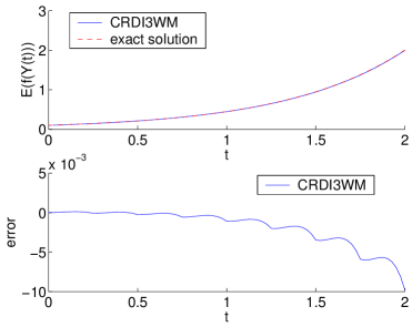
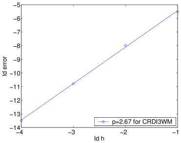
Figure 1: Scheme CRDI3WM with SDE (29).

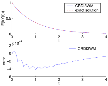
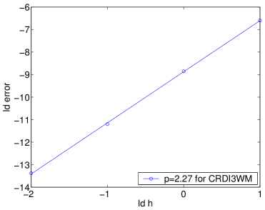
Figure 2: Scheme CRDI3WM with SDE (30).

Next, SDE (29) and SDE (30) are applied for the investigation of the order of convergence. Therefore, the trajectories are simulated with step sizes $2^{-1},\ldots,2^{-4}$ for SDE (29) and with step sizes $2^{1},\ldots,2^{-2}$ for SDE (30). As an example, we consider the error $\hat{\mu}$ at time $t=1.7$ for SDE (29) and at $t=3.8$ for SDE (30), which are not discretization points. The results are plotted on the right hand side of Figure 1 and Figure 2 with double logarithmic scale w.r.t. base two. On the axis of abscissae, the step sizes are plotted against the errors on the axis of ordinates. Consequently one obtains the empirical order of convergence as the slope of the printed lines. In the case of SDE (29) we get the order $p\approx 2.67$ and in the case of SDE (30) we get the order $p\approx 2.27$. Table 5 and Table 6 contain the corresponding values of the errors, the variances and the confidence intervals to the level 90%. The same has been done for all time points in order to determine the empirical order of convergence on the whole time interval $I$. These results are listed in Table 7 for both considered examples. The very good empirical orders of convergence confirm our theoretical results for the CSRK scheme CRDI3WM.

Table 5: Scheme CRDI3WM with SDE (29) at $t=1.7$.

$h$	$\hat{\mu}$	$\hat{\sigma}_{\mu}^{2}$	$\hat{\mu}-\Delta\hat{\mu}$	$\hat{\mu}+\Delta\hat{\mu}$
$2^{-1}$	-2.188E-02	1.146E-09	-2.189E-02	-2.187E-02
$2^{-2}$	-3.965E-03	1.705E-09	-3.975E-03	-3.956E-03
$2^{-3}$	-5.662E-04	1.715E-09	-5.760E-04	-5.564E-04
$2^{-4}$	-8.682E-05	1.746E-09	-9.672E-05	-7.691E-05

Table 6: Scheme CRDI3WM with SDE (30) at $t=3.8$.

$h$	$\hat{\mu}$	$\hat{\sigma}_{\mu}^{2}$	$\hat{\mu}-\Delta\hat{\mu}$	$\hat{\mu}+\Delta\hat{\mu}$
$2^{1}$	-1.031E-02	9.365E-12	-1.031E-02	-1.031E-02
$2^{0}$	-2.161E-03	2.294E-11	-2.162E-03	-2.160E-03
$2^{-1}$	-4.258E-04	4.453E-11	-4.274E-04	-4.242E-04
$2^{-2}$	-9.392E-05	3.375E-11	-9.530E-05	-9.255E-05

Table 7: Orders of convergence for CRDI3WM.

$SDE~{}(\ref{Simu:linear-SDE1})$
$t$	order	$t$	order
0.1	2.35	1.1	2.94
0.2	3.39	1.2	2.60
0.3	3.54	1.3	2.69
0.4	3.16	1.4	2.67
0.5	2.87	1.5	2.80
0.6	3.50	1.6	2.89
0.7	2.32	1.7	2.67
0.8	2.44	1.8	2.72
0.9	2.53	1.9	2.70
1.0	2.79	2.0	2.80

$SDE~{}(\ref{Simu:dm-SDE})$
$t$	order	$t$	order
0.2	1.82	2.2	2.30
0.4	1.84	2.4	2.27
0.6	1.95	2.6	2.24
0.8	2.07	2.8	2.24
1.0	2.13	3.0	2.22
1.2	2.26	3.2	2.25
1.4	2.32	3.4	2.26
1.6	2.36	3.6	2.27
1.8	2.37	3.8	2.27
2.0	2.31	4.0	2.24