Relativistic effects in the tidal interaction between a white dwarf and a massive
black hole in Fermi normal coordinates

Abstract

We consider tidal encounters between a white dwarf and an intermediate mass black hole. Both weak encounters and those at the threshold of disruption are modeled. The numerical code combines mesh-based hydrodynamics, a spectral method solution of the self-gravity, and a general relativistic Fermi normal coordinate system that follows the star and debris. Fermi normal coordinates provide an expansion of the black hole tidal field that includes quadrupole and higher multipole moments and relativistic corrections. We compute the mass loss from the white dwarf that occurs in weak tidal encounters. Secondly, we compute carefully the energy deposition onto the star, examining the effects of nonradial and radial mode excitation, surface layer heating, mass loss, and relativistic orbital motion. We find evidence of a slight relativistic suppression in tidal energy transfer. Tidal energy deposition is compared to orbital energy loss due to gravitational bremsstrahlung and the combined losses are used to estimate tidal capture orbits. Heating and partial mass stripping will lead to an expansion of the white dwarf, making it easier for the star to be tidally disrupted on the next passage. Finally, we examine angular momentum deposition. By including the octupole tide, we are able for the first time to calculate deflection of the center of mass of the star and debris. With this observed deflection, and taking into account orbital relativistic effects, we compute directly the change in orbital angular momentum and show its balance with computed spin angular momentum deposition.

I Introduction

The tidal disruption of a star can serve as a diagnostic for the presence of a dormant black hole in a distant galaxy rees1988 ; komo2004 . The theoretically predicted rate is $10^{-5}$ to $10^{-4}$ yr^-1 for galaxies like the Milky Way mago1999 ; wang2004 . While such tidal disruption events (TDEs) are rare, they give rise to powerful flares of emission at and above Eddington luminosity cart1982 ; rees1988 ; phin1989 ; evan1989 ; stru2009 , with spectral features and time scales that might reveal both the type of star and the mass (and perhaps spin) of the black hole. For main sequence stars disruption may occur in close encounters with supermassive black holes (SMBH) of mass $M\lesssim 10^{8}(R_{*}/R_{\odot})^{3/2}(M_{*}/M_{\odot})^{-1/2}M_{\odot}$, where $M_{*}$ and $R_{*}$ are the mass and radius of the star. With a black hole of higher mass the star will cross the event horizon before disrupting. The upper mass limit is increased if the black hole’s spin is near maximal belo1992 ; kesd2012 . Higher black hole masses are relevant for stripping red giant envelopes. Disrupting a white dwarf in contrast requires an intermediate mass black hole (IMBH) with $M\lesssim 1.8\times 10^{5}(R_{*}/0.012R_{\odot})^{3/2}(M_{*}/0.6M_{\odot})^{-1/2}M_{\odot}$.

In excess of a dozen TDE candidates have been discovered so far. A number of these have been observed in x-ray grup1999 ; komo1999 ; grei2000 ; komo2004 ; halp2004 ; esqu2007 ; capp2009 ; komo2009 ; maks2010 ; cumm2011 ; cenk2011 , with others picked up in the optical/UV renz1995 ; geza2008 ; geza2009 ; vanv2011 ; geza2012 and radio zaud2011 . Two of the most recent TDEs were detected by the Swift satellite: Swift J164449.3+573451 (hereafter Sw J1644+57) cumm2011 ; leva2011 ; bloo2011 ; burr2011 ; zaud2011 and Swift J2058.4+0516 cenk2011 . These two events have high-energy features and coincident radio emission that imply the presence of collimated relativistic jets (i.e., blazarlike activity). Another object, PS1-10jh, discovered geza2012 in the Pan-STARRS1 Medium Deep Survey, appears to have been the disruption of a helium-rich stellar core, whose red giant envelope was presumably stripped in some preceding tidal event.

A star is disrupted if its orbit reaches within the tidal radius of the black hole, given by $R_{t}\simeq R_{*}(M/M_{*})^{1/3}$. For a parabolic orbit that just reaches the tidal radius at pericenter, $R_{t}=R_{p}$, theoretical considerations indicate the star should disrupt with approximately half the debris bound to the hole and half ejected from the system. The free streaming of bound debris implies a late-time mass return rate that decays as $t^{-5/3}$ rees1988 . Early numerical models confirmed the expectations, showing a rapid rise in the mass return rate well above Eddington level before the power-law decay set in evan1989 . The precise form of the early rise and plateau is sensitive to stellar structure and effects of hydrodynamic shocks as the star undergoes disruption loda2009 . The picture is altered if the star approaches on an already bound orbit haya2012 , which affects the late time-dependence of returning mass. Moreover, stars may have orbits that result in a weak tidal encounter or that penetrate well inside the tidal radius cart1982 ; koba2004 . The strength of the encounter is often parametrized by $\eta=(R_{p}^{3}/M)^{1/2}(M_{*}/R_{*}^{3})^{1/2}$ pres1977 , or by the penetration factor $\beta=\eta^{-2/3}$ where $R_{p}=R_{t}/\beta$. In the deep plunging case $\beta\gg 1$, strong tidal compression leads to break out of a shock and a prompt x-ray flare, which comes in advance of the flare produced as captured gas streams back to the black hole after one or more orbits. Other potential observational signatures include supernovalike remnant structures associated with the ejection of debris khok1996 ; kase2010 , coincident electromagnetic and gravitational wave signals koba2004 , and possible thermonuclear runaway from severe compression of white dwarfs cart1982 ; rath2005 ; rosA2009 .

Tidal disruption has been investigated with various numerical means, including smoothed particle hydrodynamics  nolt1982 ; bick1983 ; evan1989 ; lagu1993 ; ayal2000 ; koba2004 ; loda2009 , mesh-based finite difference or spectral methods khok1993 ; khok1993strong ; frol1994 ; marc1996 ; dien1997 ; guil2009 , and affine models cart1982 ; cart1983 ; lumi1986 ; koch1992 ; ivan2001 ; ivan2003 . Numerical modeling of radiative processes is also important for understanding how TDEs appear in multiple wave bands bogd2004 and in accounting for nonadiabatic effects on the dynamics. In TDEs that involve white dwarfs, the close approach to the black hole requires handling general relativistic effects frol1994 ; dien1997 ; haas2012 . Moreover, new observations continue to bring surprises, such as the unanticipated rapid formation of relativistic jets and synchrotron radio emission bloo2011 associated with Sw 1644+57. These observations point to the need to include magnetohydrodynamics in models as well (see arguments in Ref. shch2012 ).

The Sw 1644+57 event is generally thought to represent tidal disruption of a main sequence star by a $10^{6}$ to $10^{7}M_{\odot}$ SMBH bloo2011 ; burr2011 ; leva2011 ; zaud2011 . An alternative model, however, posits that the observed short time scales and multiple bursts can be best explained via the disruption of a white dwarf by an IMBH krol2011 ; krol2012 in multiple passes. Whatever the case may be with Sw 1644+57, because of the shorter time scales and higher mass return rate, it has been argued that white dwarf TDEs may end up being frequently observed in future flux-limited surveys shch2012 .

In this paper our focus is on encounters between white dwarfs and IMBHs, with primary attention devoted to events at threshold for disruption ($\eta\simeq 1$) or weaker ($\eta>1$). We are particularly interested in (1) computing partial mass loss in weaker encounters, (2) calculating accurately energy and angular momentum deposition, (3) observing relativistic effects, and (4) determining the capture orbits of white dwarfs after their initial passage. To this end, we have constructed a new numerical code whose central feature is use of Fermi normal coordinates (FNCs) ishi2005 . In FNCs the spacetime geometry of the black hole is expanded in the vicinity of a timelike geodesic that approximately tracks the center of mass (CM) motion of the star (and debris). Our approach is similar to Ref. frol1994 but differs in the use of a higher-order expansion of the tidal field, which includes higher moments and relativistic corrections.

Despite relativistic orbital motion, these coordinates allow use of Newtonian hydrodynamics and self-gravity within the FNC domain. By not including post-Newtonian (PN) corrections to the stellar self-gravity and hydro, a floor is set on the accuracy ($\simeq 10^{-4}$) of the model. Nevertheless, we show that octupole and $l=4$ moments can be significant, as well as several orbital PN corrections. Hydrodynamics is computed using a piece-wise parabolic method (PPM) Lagrangian remap code (PPMLR). The self-gravitational field is obtained using three-dimensional fast Fourier transforms. The code runs on cluster computers and each of our three-dimensional simulations is run at several resolutions to confirm numerical convergence. Since the size of the FNC domain is necessarily limited, there is a limit on how long a disrupted star or stripped gas can be followed. In principle, however, our simulations can serve as initial conditions for a second code that would calculate the return of gas to the black hole and formation of an accretion disk.

This paper is organized as follows. In Sec. II the formalism is presented for including relativistic effects and higher moments in tidal interactions. We give an orbital PN expansion of the tidal field and consider the order of magnitude significance of various terms. Tidal field moments through $l=4$ might be significant. Similarly, (orbital) PN corrections to $l=2$ and $l=3$, as well as the gravitomagnetic potential, might be significant. The fluid equations of motion are given with this level of approximation. We discuss our numerical results in Secs. III through VI, relegating to Appendix A description of the numerical hydrodynamics and self-gravity methods. Section III details our initial stellar model and the range of inbound orbits we consider. Section IV discusses the overall hydrodynamic features and shows the amount of mass loss from a white dwarf during various weak tidal encounters. For TDEs considered here, we found the $l=4$ moment to have negligible impact. The situation with the gravitomagnetic potential is subtle, and we intend to address it in a subsequent paper. In Sec. V we consider energy deposition onto the star and energy loss from the orbit. We discuss the combined effects of nonradial and radial mode excitation, surface layer heating, mass loss, relativistic orbital motion, and gravitational bremsstrahlung. Section VI presents results on deposition of angular momentum (spin) onto the star. By including the octupole tide, we show in Sec. VI.1 the computed tidal deflection of the CM and, with relativistic effects accounted for, relate it to the reduction of orbital angular momentum. In Sec. VII we summarize our conclusions. Appendix B gives the form of the octupole tidal field.

Throughout this paper, where relativity is concerned, we use the sign conventions and notation of Misner et al. misn1973 . We use geometrical units in which $c=G=1$ and scale all dimensional quantities relative to the black hole mass $M$, except where otherwise indicated in discussing astrophysical consequences.

II Formalism

Fermi normal coordinates provide a convenient local moving frame for calculating relativistic tidal encounters. The FNC formalism was first developed by Manasse and Misner mana1963 (see additional work by Mashhoon mash1975 and Marck marc1983 ). In more recent work, the metric was expanded through fourth order in the spatial distance from the geodesic by Ishii et al. ishi2005 . The result is a tidal field rich in multipoles and relativistic terms. Here we specialize to a Schwarzschild background and summarize the coordinate system and the tidal field expansion. We also consider physical scales associated with application to white dwarf/IMBH encounters and address use of Newtonian self-gravity and hydrodynamics in the FNC frame. This approximation, adequate for white dwarfs, affects which terms in the relativistic tidal field are worth consistently retaining.

II.1 Fermi normal coordinates

Fermi normal coordinates rely upon using local flatness in the vicinity of a freely falling observer over an extended period of time. Consider an arbitrary spacetime with coordinates $X^{\mu}$ and a timelike geodesic $\mathcal{G}$ described by $X^{\mu}(\tau)$, parametrized by proper time $\tau$. The tangent vector is $\mathbf{u}=\partial/\partial\tau$. Greek indices label these arbitrary four-dimensional coordinates and coordinate components of tensors in this system. The second (FNC) coordinate system $x^{a}=(\tau,x^{i})$ has its spatial origin fixed to move along the trajectory $\mathcal{G}$ mana1963 ; pois2004 , with the conditions

$$g_{ab}|_{\mathcal{G}}=\eta_{ab},\qquad\Gamma^{a}_{\ bc}|_{\mathcal{G}}=0,$$ (1)

enforced at all times. Here latin indices beginning with $a,b,c,\ldots$ label the four new coordinates and components in this frame. Latin indices beginning with $i,j,k,\ldots$ are reserved for FNC spatial coordinates. Let $\mathcal{P}_{0}$ be the single event on the geodesic $\mathcal{G}$ at $\tau=0$. Construct an orthonormal tetrad $\boldsymbol{\lambda}_{a}=(\boldsymbol{\lambda}_{0},\boldsymbol{\lambda}_{1},\boldsymbol{\lambda}_{2},\boldsymbol{\lambda}_{3})$ at this point. Choose $\boldsymbol{\lambda}_{0}=\mathbf{u}$, making the tangent vector the timelike member of the tetrad at $\mathcal{P}_{0}$. The remaining tetrad elements at $\mathcal{P}_{0}$ are spacelike. Now extend the basis by parallel transporting the tetrad $\boldsymbol{\lambda}_{a}$ along $\mathcal{G}$. One condition is identically satisfied, since $\nabla_{\mathbf{u}}\boldsymbol{\lambda}_{0}=\nabla_{\mathbf{u}}\mathbf{u}=0$. Imposing $\nabla_{\mathbf{u}}\boldsymbol{\lambda}_{i}=0$ on the spacelike elements $\boldsymbol{\lambda}_{i}$ defines the tetrad in the future and past of $\mathcal{P}_{0}$. With the moving tetrad defined on $\mathcal{G}$, each element $\boldsymbol{\lambda}_{i}$ of the triad is used at any constant time $\tau$ to launch spacelike geodesics from $\mathcal{P}(\tau)$. The proper distance along each of these three curves defines the spatial coordinates $x^{i}$. Thus $\boldsymbol{\lambda}_{i}=\partial/\partial x^{i}$. The proper time $\tau$ along the geodesic completes the coordinate system: $x^{0}=\tau$.

The conditions (1) further imply that all time derivatives of the connection and of the first derivative of the metric vanish along $\mathcal{G}$: $\Gamma^{a}_{\ bc,0}=\Gamma^{a}_{\ bc,00}=0$, etc, and $g_{ab,c0}=g_{ab,c00}=0$, etc. This implies mana1963 ; pois2004 ; ishi2005 that the metric may be expanded in a power series in spatial distance of the form

$$g_{ab} = \eta_{ab}+\tfrac{1}{2}g_{ab,ij}(\tau)x^{i}x^{j}+\tfrac{1}{6}g_{ab,ijk}(\tau)x^{i}x^{j}x^{k}$$ (2)

$$+\tfrac{1}{24}g_{ab,ijkl}(\tau)x^{i}x^{j}x^{k}x^{l}+\mathcal{O}(x^{5}).$$

The coefficients involve spatial derivatives of the metric only and are functions of just the FNC time coordinate $\tau$.

The specific form of the Taylor coefficients depends on how the tetrad is extended away from $\mathcal{G}$ but will in any case involve the Riemann tensor and its derivatives evaluated on the geodesic as functions of $\tau$. The expansion was derived to quadratic order by Manasse and Misner mana1963 and was extended to fourth order by Ishii et al. ishi2005 . Gathering results in the latter paper, we find

$$g_{00} = -1-C_{ij}\,x^{i}x^{j}-\frac{1}{3}C_{ijk}\,x^{i}x^{j}x^{k}-\frac{1}{12}\left(C_{ijkl}+4C_{(ij}C_{kl)}-4B_{(kl|n|}{B_{ij)}}^{n}\right)x^{i}x^{j}x^{k}x^{l}+\mathcal{O}\left(|\vec{x}|^{5}/\mathcal{R}^{5}\right),$$ (3)

$$g_{0m} = \frac{2}{3}B_{ijm}\,x^{i}x^{j}+\frac{1}{4}R_{m(ij|0|;k)}\,x^{i}x^{j}x^{k}$$ (4)

$$\qquad+\frac{1}{135}\left(9R_{m(ij|0|;kl)}-6R_{m(ij}^{\ \ \ \ \ 0}R_{|0|kl)0}-2R_{m(ij}^{\ \ \ \ \ n}R_{|n|kl)0}\right)x^{i}x^{j}x^{k}x^{l}+\mathcal{O}\left(|\vec{x}|^{5}/\mathcal{R}^{5}\right),$$

$$g_{mn} = \delta_{mn}+\frac{1}{6}\left(R_{imnj}+R_{inmj}\right)x^{i}x^{j}-\frac{1}{36}\left(R_{injm;k}+R_{inkm;j}+R_{jnim;k}+R_{knim;j}+R_{knjm;i}+R_{jnkm;i}\right)x^{i}x^{j}x^{k}$$ (5)

$$\qquad+\frac{1}{180}\left(9R_{m(ij|n|;kl)}-6R_{m(ij}^{\ \ \ \ \ 0}R_{|n|kl)0}-2R_{m(ij}^{\ \ \ \ \ p}R_{|n|kl)p}\right)x^{i}x^{j}x^{k}x^{l}+\mathcal{O}\left(|\vec{x}|^{5}/\mathcal{R}^{5}\right),$$

where the following tidal tensor definitions,

$$C_{ij} \equiv R_{0i0j}, \qquad C_{ijk} \equiv R_{0(i|0|j;k)},$$

$$C_{ijkl} \equiv R_{0(i|0|j;kl)}, \qquad B_{ijk} \equiv R_{k(ij)0},$$ (6)

have been used. We refer to $C_{ij}$, $C_{ijk}$, and $C_{ijkl}$ as the quadrupole, octupole, and $l=4$ tides, respectively. The quadrupole tide is the electric part $\mathscr{E}_{ij}$ of the Riemann tensor, while $B_{ijk}$ is related to the magnetic part $\mathscr{B}_{ij}$ of the Riemann tensor. The latter further gives rise to the gravitomagnetic potential thor1985

$$A_{k}=\tfrac{2}{3}B_{ijk}x^{i}x^{j},$$ (7)

which will appear in the fluid equations of motion. In the metric expansion, $\mathcal{R}$ is a (smallest) length scale associated with the inhomogeneity and curvature length scales of the surrounding spacetime. Also, the usual notation has been used misn1973 that parentheses bracketing indices indicate symmetrization with respect to all enclosed indices, e.g.,

$$A_{(ij)} = \tfrac{1}{2}(A_{ij}+A_{ji}),$$ (8)

$$A_{(ijk)} = \tfrac{1}{6}\left(A_{ijk}+A_{jik}+A_{jki}+A_{kji}+A_{kij}+A_{ikj}\right),$$

excluding, however, any that are enclosed by vertical strokes.

We see that this coordinate system provides an expansion of the metric provided the Riemann tensor $R_{abcd}$ and its derivatives in the FNC are known. Fortunately, the Riemann tensor and derivatives are only required along $\mathcal{G}$ and need only be known in some coordinate system (e.g., $R_{\mu\alpha\nu\beta}$). The two are linked by a coordinate transformation and the original coordinate components of the tetrad vectors yield the Jacobian matrix along $\mathcal{G}$: $\lambda_{a}^{\ \mu}=\partial X^{\mu}/\partial x^{a}|_{\mathcal{G}}$. Thus we easily find

$$R_{abcd} = R_{\mu\alpha\nu\beta}\ \lambda^{\ \mu}_{a}\ \lambda^{\ \alpha}_{b}\ \lambda^{\ \nu}_{c}\ \lambda^{\ \beta}_{d},$$ (9)

$$R_{abcd;e} = R_{\mu\alpha\nu\beta;\rho}\ \lambda^{\ \mu}_{a}\ \lambda^{\ \alpha}_{b}\ \lambda^{\ \nu}_{c}\ \lambda^{\ \beta}_{d}\ \lambda^{\ \rho}_{e},$$

$$R_{abcd;ef} = R_{\mu\alpha\nu\beta;\rho\sigma}\ \lambda^{\ \mu}_{a}\ \lambda^{\ \alpha}_{b}\ \lambda^{\ \nu}_{c}\ \lambda^{\ \beta}_{d}\ \lambda^{\ \rho}_{e}\ \lambda^{\ \sigma}_{f}.$$

II.2 Geodesic motion on Schwarzschild spacetime and construction of the FNC frame

The coordinates $X^{\mu}$ can be taken to be standard Schwarzschild coordinates $(t,r,\theta,\phi)$. The line element is

$$ds^{2}=-fdt^{2}+f^{-1}dr^{2}+r^{2}\left(d\theta^{2}+\sin^{2}\theta d\phi^{2}\right),$$ (10)

with $f(r)=1-2M/r$. Test body orbits have two constants of motion

$$-\tilde{E}=U_{t},\qquad\qquad\tilde{L}=U_{\phi},$$ (11)

where $\tilde{E}$ is the specific orbital energy and $\tilde{L}$ is the specific angular momentum. We confine the motion to the equatorial plane and have first-order equations of motion

$$\frac{dt}{d\tau}=\frac{\tilde{E}}{f(r)},\quad\frac{d\phi}{d\tau}=\frac{\tilde{L}}{r^{2}},\quad\left(\frac{dr}{d\tau}\right)^{2}=\tilde{E}^{2}-V(r),$$ (12)

where $V\equiv f(1+\tilde{L}^{2}/r^{2})$ is the effective potential for radial motion. Marginally bound orbits have $\tilde{E}=1$.

To integrate an arbitrary geodesic we use the parametrization of Darwin darw1959 (see also cutl1994 ). A semilatus rectum $p$ and eccentricity $e$ are defined, along with a radial phase angle $\chi$, defined by

$$r(\chi)=\frac{pM}{1+e\cos\chi}.$$ (13)

Let $r_{1}$ represent periastron and $r_{2}$ be apastron. We find

$$r_{1}=\frac{pM}{1+e},\qquad\qquad r_{2}=\frac{pM}{1-e}.$$ (14)

Either pair of parameters can be used to specify a bound orbit. Similarly, we can make the connection

$$\tilde{E}^{2} = \frac{(p-2-2e)(p-2+2e)}{p(p-3-e^{2})},$$ (15)

$$\tilde{L}^{2} = \frac{p^{2}M^{2}}{p-3-e^{2}}.$$ (16)

In terms of $\chi$, Eqs. (12) take the form

$$\frac{dt}{d\chi} = \frac{p^{2}M}{(p-2-2e\cos\chi)(1+e\cos\chi)^{2}}$$ (17)

$$\quad\times\left[\frac{(p-2)^{2}-4e^{2}}{p-6-2e\cos\chi}\right]^{1/2},$$

$$\frac{d\phi}{d\chi} = p^{1/2}\left(p-6-2e\cos\chi\right)^{-1/2},$$ (18)

$$\frac{d\tau}{d\chi} = \frac{p^{3/2}M}{\left(1+e\cos\chi\right)^{2}}\left(\frac{p-3-e^{2}}{p-6-2e\cos\chi}\right)^{1/2}.\quad$$ (19)

The benefit of the curve parameter $\chi$ is in removing singularities from the integration at radial turning points. We are thus able to consider tidal encounters of a system already in a bound orbit or, with suitable redefinition of parameters, hyperbolic systems with $\tilde{E}>1$. We are principally interested in $\tilde{E}=1$ orbits. For these we have $e=1$ and define $r_{1}\equiv R_{p}$. Then $r_{2}\rightarrow\infty$ and

$$pM=2R_{p},\qquad\qquad\tilde{L}^{2}=\frac{p^{2}M^{2}}{p-4}.$$ (20)

Once an orbit is adopted we can construct the Fermi normal frame vectors. The vectors must satisfy the orthonormality condition $\lambda_{a}^{\ \mu}\lambda_{b}^{\ \nu}g_{\mu\nu}=\eta_{ab}$. After selecting $\lambda_{0}^{\ \mu}=U^{\mu}$, a second natural choice is to take one spatial vector pointing out of the equatorial plane: $\lambda_{2}^{\ \mu}=(0,0,1/r,0)$. Following Marck marc1983 , we can construct two more vectors, $\tilde{\lambda}_{1}^{\ \mu}$ and $\tilde{\lambda}_{3}^{\ \mu}$, that make an orthonormal set with $\lambda_{0}^{\ \mu}$ and $\lambda_{2}^{\ \mu}$,

$$\lambda_{0}^{\ \mu} = \left(\frac{\tilde{E}}{f},U^{r},0,\frac{\tilde{L}}{r^{2}}\right),$$ (21)

$$\tilde{\lambda}_{1}^{\ \mu} = \left(\frac{U^{r}r}{f\sqrt{r^{2}+\tilde{L}^{2}}},\frac{r\tilde{E}}{\sqrt{r^{2}+\tilde{L}^{2}}},0,0\right),$$

$$\lambda_{2}^{\ \mu} = \left(0,0,\frac{1}{r},0\right),$$

$$\tilde{\lambda}_{3}^{\ \mu} = \left(\frac{\tilde{E}\tilde{L}}{f\sqrt{r^{2}+\tilde{L}^{2}}},\frac{U^{r}\tilde{L}}{\sqrt{r^{2}+\tilde{L}^{2}}},0,\frac{\sqrt{r^{2}+\tilde{L}^{2}}}{r^{2}}\right).$$

While orthonormal, it may be shown that $\tilde{\lambda}_{1}^{\ \mu}$ and $\tilde{\lambda}_{3}^{\ \mu}$ do not satisfy the parallel transport condition

$$U^{\nu}\partial_{\nu}\lambda_{a}^{\ \mu}+\Gamma^{\mu}_{\ \alpha\beta}U^{\alpha}\lambda_{a}^{\ \beta}=0.$$ (22)

We can, however, form two new vectors, $\lambda_{1}^{\ \mu}$ and $\lambda_{3}^{\ \mu}$, via a purely spatial rotation,

$$\lambda_{1}^{\ \mu} = \tilde{\lambda}_{1}^{\ \mu}\cos\Psi-\tilde{\lambda}_{3}^{\ \mu}\sin\Psi,$$

$$\lambda_{3}^{\ \mu} = \tilde{\lambda}_{1}^{\ \mu}\sin\Psi+\tilde{\lambda}_{3}^{\ \mu}\cos\Psi,$$ (23)

and then attempt to enforce the parallel transport condition on these. This proves possible as long as the frame precesses at a rate given by

$$\frac{d\Psi}{d\tau}=\frac{\tilde{E}\tilde{L}}{r^{2}+\tilde{L}^{2}}.$$ (24)

For a chosen value of $\tilde{L}$ and $\tilde{E}=1$, we have an orthonormal tetrad parallel transported along a parabolic geodesic.

II.3 Tidal tensor components and orbital PN expansion

In Schwarzschild coordinates the components of the Riemann tensor are

$$R_{trtr} =-\frac{2M}{r^{3}}, R_{t\theta t\theta} =\frac{Mf}{r},$$

$$R_{t\phi t\phi} =\frac{Mf}{r}\sin^{2}\theta, R_{r\theta r\theta} =-\frac{M}{rf},$$

$$R_{r\phi r\phi} =-\frac{M}{rf}\sin^{2}\theta, \quad R_{\theta\phi\theta\phi} =2Mr\sin^{2}\theta,$$ (25)

with other nonzero components following from the symmetries $R_{\mu\alpha\nu\beta}=-R_{\mu\alpha\beta\nu}=-R_{\alpha\mu\nu\beta}=+R_{\nu\beta\mu\alpha}$ and with all other elements vanishing. The first and second covariant derivatives are readily computed. We may then use Eq. (9) to project the Riemann tensor and its covariant derivatives (and thus the various tidal tensors). In fact, we have a choice. We can use $\{\boldsymbol{\lambda}_{0},\boldsymbol{\lambda_{1}},\boldsymbol{\lambda}_{2},\boldsymbol{\lambda_{3}}\}$ to express components in the FNC frame or use $\{\boldsymbol{\lambda}_{0},\boldsymbol{\tilde{\lambda}_{1}},\boldsymbol{\lambda}_{2},\boldsymbol{\tilde{\lambda}_{3}}\}$ to cast tensor components into the noninertial frame. It is convenient to consider both.

To distinguish tidal tensors in the FNC frame from those in the noninertial frame, the latter carry a tilde: $\tilde{C}_{ij}$, $\tilde{C}_{ijk}$, $\tilde{C}_{ijkl}$, and $\tilde{B}_{ijk}$). To obtain $\tilde{A}_{k}$, we also have to rotate the coordinates,

$$\tilde{x}^{1} = x^{1}\cos\Psi+x^{3}\sin\Psi,$$

$$\tilde{x}^{2} = x^{2},$$

$$\tilde{x}^{3} = -x^{1}\sin\Psi+x^{3}\cos\Psi.$$ (26)

The tilde frame, while not parallel-propagated, affords a simpler form for the tidal tensors. The quadrupole tidal tensor in the noninertial frame is diagonal, with

$$\tilde{C}_{11} = -\frac{2M}{r^{3}}\left(1+\frac{3\tilde{L}^{2}}{2r^{2}}\right),$$

$$\tilde{C}_{22} = \frac{M}{r^{3}}\left(1+\frac{3\tilde{L}^{2}}{r^{2}}\right),$$

$$\tilde{C}_{33} = \frac{M}{r^{3}}.$$ (27)

In contrast, the nonzero components in the FNC frame are

$$C_{11} = \frac{M}{r^{3}}\left[\left(1-3\cos^{2}\Psi\right)-\frac{3\tilde{L}^{2}}{r^{2}}\cos^{2}\Psi\right],$$

$$C_{13} = C_{31}=-\frac{3M}{r^{3}}\left(1+\frac{\tilde{L}^{2}}{r^{2}}\right)\sin\Psi\cos\Psi,$$

$$C_{22} = \frac{M}{r^{3}}\left(1+\frac{3\tilde{L}^{2}}{r^{2}}\right),$$

$$C_{33} = \frac{M}{r^{3}}\left[\left(1-3\sin^{2}\Psi\right)-\frac{3\tilde{L}^{2}}{r^{2}}\sin^{2}\Psi\right].$$ (28)

Likewise, the nonzero components of the octupole tidal tensor are simpler in the noninertial frame,

$$\tilde{C}_{111} = \frac{6M}{r^{4}}\left(1+\frac{3\tilde{L}^{2}}{2r^{2}}\right)V_{2}^{-1},$$

$$\tilde{C}_{131} = \tilde{C}_{311}=\tilde{C}_{113}=\frac{4M}{r^{4}}\frac{\tilde{L}}{r}U^{r}\left(1+\frac{5\tilde{L}^{2}}{4r^{2}}\right)V_{2}^{-1},$$

$$\tilde{C}_{122} = \tilde{C}_{212}=\tilde{C}_{221}=-\frac{3M}{r^{4}}\left(1+\frac{7\tilde{L}^{2}}{3r^{2}}\right)V_{2}^{-1},$$

$$\tilde{C}_{133} = \tilde{C}_{313}=\tilde{C}_{331}=-\frac{3M}{r^{4}}\left(1+\frac{2\tilde{L}^{2}}{3r^{2}}\right)V_{2}^{-1},$$

$$\tilde{C}_{322} = \tilde{C}_{232}=\tilde{C}_{223}=-\frac{M}{r^{4}}\frac{\tilde{L}}{r}U^{r}\left(1+\frac{5\tilde{L}^{2}}{r^{2}}\right)V_{2}^{-1},$$

$$\tilde{C}_{333} = -\frac{3M}{r^{4}}\frac{\tilde{L}}{r}U^{r}\,V_{2}^{-1},$$ (29)

where $V_{2}\equiv\sqrt{1+\tilde{L}^{2}/r^{2}}$ (notation of Ishii et al. ishi2005 ). The octupole tidal tensor in the FNC frame is somewhat more complicated and we list its components in Appendix B.

We have also obtained the lengthy expressions for $\tilde{C}_{ijkl}$ and $C_{ijkl}$ using MATHEMATICA but in the interests of brevity omit reproducing them here. We confirm the expressions found in ishi2005 with the exception of $\tilde{C}_{2233}$ in Eq. (B22), which should not have an overall minus sign.

The nonzero components of $\tilde{B}_{ijk}$ in the noninertial frame are given by

$$\tilde{B}_{131} = \tilde{B}_{311}=-\tilde{B}_{232}=-\tilde{B}_{322}=-\tfrac{1}{2}\tilde{B}_{113}=\tfrac{1}{2}\tilde{B}_{223}$$ (30)

$$= -\frac{3M}{2r^{3}}\,\frac{\tilde{L}}{r}\,V_{2}.$$

In the FNC frame we have instead

$$B_{131} = B_{311}=-B_{232}=-B_{322}=-\tfrac{1}{2}B_{113}=\tfrac{1}{2}B_{223}$$ (31)

$$= -\frac{3M}{2r^{3}}\,\frac{\tilde{L}}{r}\,V_{2}\cos\Psi,$$

$$B_{122} = -B_{133}=B_{212}=-\tfrac{1}{2}B_{221}=-B_{313}=\tfrac{1}{2}B_{331}$$ (32)

$$= -\frac{3M}{2r^{3}}\,\frac{\tilde{L}}{r}\,V_{2}\sin\Psi.$$

From these we derive the components of the gravitomagnetic potential. In the FNC frame we find

$$A_{1} = -\frac{2M}{r^{3}}\,\frac{\tilde{L}}{r}\,V_{2}\,\Big{\{}x^{1}x^{3}\cos\Psi+\left[(x^{3})^{2}-(x^{2})^{2}\right]\sin\Psi\Big{\}},$$

$$A_{2} = \frac{2M}{r^{3}}\,\frac{\tilde{L}}{r}\,V_{2}\,x^{2}\left(x^{3}\cos\Psi-x^{1}\sin\Psi\right),$$ (33)

$$A_{3} = \frac{2M}{r^{3}}\,\frac{\tilde{L}}{r}\,V_{2}\,\Big{\{}\left[(x^{1})^{2}-(x^{2})^{2}\right]\cos\Psi+x^{1}x^{3}\sin\Psi\Big{\}}.$$

For all but the most relativistic orbits, the spatial components of the four-velocity will be small compared to unity, $|U^{r}|\sim|r\,U^{\phi}|\lesssim 1$. We can denote the maximum velocity scale at pericenter by $\delta$ and set

$$\delta=\left(\frac{M}{R_{p}}\right)^{1/2}.$$ (34)

Assuming $\delta$ is sufficiently small, we can use it as the basis for making an orbital PN expansion. The various tidal tensors have been written in a suggestive way, since $\tilde{L}/r\sim|U^{\hat{i}}|\lesssim\mathcal{O}(\delta)$. We can expand the tidal tensors in the following way

$$C_{ij} = C_{ij}^{(0)}+C_{ij}^{(1)},$$ (35)

$$C_{ijk} = C_{ijk}^{(0)}+C_{ijk}^{(1)}+C_{ijk}^{(2)}+\cdots,$$ (36)

$$C_{ijkl} = C_{ijkl}^{(0)}+C_{ijkl}^{(1)}+C_{ijkl}^{(2)}+\cdots,$$ (37)

where the leading terms represent the Newtonian limit (e.g., $C_{ij}^{(0)}=\partial_{i}\partial_{j}\Phi_{bh}$, $C_{ijk}^{(0)}=\partial_{i}\partial_{j}\partial_{k}\Phi_{bh}$, etc). Higher-order terms ($C_{ij\ldots}^{(n)}$) are orbital PN corrections and are $\mathcal{O}(\delta^{2n})$ relative to the Newtonian limit. A similar story holds for $B_{ijk}$ and $A_{k}$ except their expansions start at $\mathcal{O}(\delta)$,

$$B_{ijk} = B_{ijk}^{(0.5)}+B_{ijk}^{(1.5)}+\cdots,$$ (38)

$$A_{k} = A_{k}^{(0.5)}+A_{k}^{(1.5)}+\cdots.$$ (39)

We see that we could reexpress the metric given in Eqs. (3)–(5) as simultaneous power series in $\nu=|\vec{x}|/\mathcal{R}$ and $\delta$.

II.4 Self-gravity of the star combined with the external tidal field

Ishii et al. ishi2005 derived the third- and fourth-order terms in the tidal field, which are summarized above, and used the expansion along with a Newtonian stellar model to study tidal effects on a star in circular orbit about a Kerr black hole. In this section and the next we provide a justification for use of Newtonian self-gravity and hydrodynamics (see also fish1973 ), estimate the resulting errors, and determine what parts of the tidal field expansion should be consistently retained. This approximation is adequate for main sequence stars and white dwarfs, but much less so for neutron stars.

Consider a star of mass $M_{*}$ that encounters a more massive black hole of mass $M$. We are concerned with mass ratios in the range

$$\mu\equiv\frac{M_{*}}{M}\sim 10^{-5}\text{--}10^{-3},$$ (40)

corresponding to black holes with masses $M\sim 10^{3}-10^{5}M_{\odot}$. Let the stellar radius be $R_{*}$. The strength of the tidal encounter is determined by

$$\eta=\left(\frac{R_{p}^{3}}{M}\frac{M_{*}}{R_{*}^{3}}\right)^{1/2}.$$ (41)

In this paper we restrict attention to stars that just reach the tidal radius at pericenter and disrupt ($\eta\simeq 1$) and to weaker, partially disruptive encounters ($\eta\sim 2-6$).

The metric given in Eqs. (3)–(5) would serve to compute near $\mathcal{G}$ motion of test bodies or of a fluid of negligible mass. A star with finite mass will necessarily alter the geometry. Even for a star with strong gravity, the tidal field expansion is still useful provided the star is sufficiently isolated. This requires a buffer region whose radius is small compared to the characteristic length scale of the tidal field but large compared to the compact object, so that self-gravity is also weak within the buffer region thor1985 . If the star is approximately Newtonian, the latter condition is satisfied throughout the star and the self-gravity ($\Phi_{*}$) and tidal fields will linearly superpose to lowest order and can be computed separately. We only require then that the domain of interest have a size $\mathcal{L}\gtrsim R_{*}$ small compared to the characteristic length scale of the tidal field. The assumption (40) on the mass ratio makes this possible, since

$$\frac{R_{*}}{r(t)}\lesssim\frac{R_{*}}{R_{p}}=\mu^{1/3}\,\eta^{-2/3}\ll 1.$$ (42)

Likewise, the fluid is assumed to be well modeled by Newtonian hydrodynamics (as seen in the FNC frame). Prior to tidal encounter, the star has vanishing or minimal internal fluid velocities in this frame. The internal stellar sound speed $a_{s}$ and stresses will be small and comparable to the self-gravity,

$$a_{s}^{2}\simeq\frac{p}{\rho}\lesssim|\Phi_{*}|\simeq\varepsilon^{2}=\frac{M_{*}}{R_{*}}\ll 1,$$ (43)

where $\rho$ is the rest mass density, $p$ is the isotropic pressure, and $\varepsilon$ is the (stellar) PN velocity scale. Post encounter, fluid velocities will also be small (e.g., a few multiples of stellar escape speed $|v^{i}|\simeq\varepsilon$) and subrelativistic provided the region of interest is restricted in size. In our models, we take the domain size to be

$$\mathcal{L}\lesssim 8\times R_{*}.$$ (44)

For a star immersed in an external tidal field we expect the gravitational field to take the form

$$g_{ab}=\eta_{ab}+h_{ab}^{\text{tidal}}+h_{ab}^{*}+h_{ab}^{IC}.$$ (45)

The self-gravity $h_{ab}^{*}$ depends only on the Newtonian potential $\Phi_{*}$ and is weak, $|h_{ab}^{*}|\ll 1$. The tidal field $h_{ab}^{\text{tidal}}$, as seen in FNC, is determined by equations (3)-(5) and for $|\vec{x}|\lesssim\mathcal{R}$ is also weak. The full metric must satisfy the Einstein field equations and their nonlinearity requires that a term $h_{ab}^{IC}$ be present that represents the field interaction and higher-order self-gravity corrections. In the absence of the tidal field we would have

$$h_{00}^{*} = -2\Phi_{*}+\mathcal{O}(\varepsilon^{4}),$$ (46)

$$h_{0i}^{*} = \mathcal{O}(\varepsilon^{3}),$$

$$h_{ij}^{*} = \mathcal{O}(\varepsilon^{2}),$$

where the Newtonian potential satisfies

$$\nabla^{2}\Phi_{*}=4\pi\rho,$$ (47)

and where the missing corrections are (stellar) 1PN terms. Neglect of these corrections sets a floor on the accuracy of our method. In white dwarf/IMBH encounters, most white dwarfs will have $M_{*}/R_{*}\simeq 10^{-4}$, so that $\varepsilon\simeq 0.01$. Thus, our method has intrinsic relative errors at the level of $10^{-4}$. In what follows, in analyzing $h_{ab}^{\text{IC}}$ and $h_{ab}^{\text{tidal}}$, we neglect any term whose contribution to the fluid acceleration is at or below this error level.

We have defined two small velocity parameters, $\delta$ and $\varepsilon$. These two scales are not necessarily comparable. They are related by

$$\delta=\varepsilon\,\mu^{-1/3}\,\eta^{-1/3},$$ (48)

and for a small mass ratio $\mu$ we find $\delta\gg\varepsilon$. As an example, in our application with $\varepsilon\simeq 10^{-2}$, if we take $\mu=10^{-4}$ and $\eta=1$, we have a much higher orbital velocity scale: $\delta\simeq 0.22$. This highlights one of the real advantages of Fermi normal coordinates. We could never use Newtonian hydrodynamics in a frame fixed with respect to the black hole. In combining self-gravity and the tidal field, the simultaneous expansions in $\delta$ and $\varepsilon$ make (orbital) and (stellar) PN contributions, respectively.

The external tidal field has a radius of curvature $\mathscr{R}$, an inhomogeneity scale $\mathscr{L}$, and a time scale for changes in curvature $\mathscr{T}$ thor1985 . Each of these scales is time dependent as viewed from the FNC frame center. They reach their minima at pericenter

$$\mathscr{L}\simeq R_{p},\quad\mathscr{R}\simeq\mathscr{T}\simeq\left(\frac{R_{p}^{3}}{M}\right)^{1/2},$$ (49)

where $\mathscr{L}/\mathscr{T}=\delta$. The tidal field is dominated by the quadrupole moment, which reaches a maximum of $|C_{ij}|\simeq|C_{ij}^{(0)}|\simeq\mathscr{R}^{-2}\lesssim M/R_{p}^{3}$. The star’s self-gravity is dominated by its mass monopole. At pericenter, for encounters near threshold for disruption ($\eta\simeq 1$), there is a near balance between the quadrupole tidal term and the star’s gravitational potential:

$$|C_{ij}^{(0)}\,x^{i}x^{j}|\simeq\frac{M}{R_{p}^{3}}R_{*}^{2}=\varepsilon^{2}\eta^{-2}\lesssim\varepsilon^{2}\simeq|\Phi_{*}|.$$ (50)

The size of the gravitational field correction $h_{ab}^{IC}$ can now be estimated without a full calculation. Substituting (45) into the Einstein field equations would yield a nonlinear contribution no larger than

$$\left|h_{ab}^{IC}\right|\lesssim\left|h_{00}^{*}\right|\,\left|h_{00}^{\text{tidal}}\right|\simeq\frac{M_{*}}{R_{*}}\frac{M}{R_{p}^{3}}\,R_{*}^{2}\simeq\varepsilon^{4}\eta^{-2}\lesssim\varepsilon^{4}.$$ (51)

Thus the interaction terms are formally at or below the size of the (stellar) 1PN corrections, which we have already chosen to neglect, and can be dropped as well.

At our level of approximation the metric in (45) is just the sum of Newtonian self-gravity and the FNC tidal field, but with two caveats. The first involves the assumption of a stationary black hole background. While suitable for test-body motion, the finite mass of the white dwarf will cause the black hole to wobble relative to a common center. This $\mathcal{O}(\mu)$ correction is easily dealt with in Newtonian mechanics. In relativity one could in principle treat this effect as a conservative perturbation in the black hole’s gravitational field detw2004 and correct the motion of the FNC frame and the tidal terms. Alternatively, we could use a PN calculation of the two-body orbit, and then calculate the tidal field. We have done neither, which introduces an added small source of relative error of magnitude $\sim\mu$.

The second caveat is that not all of the terms in the tidal field in (3)-(5) are significant given our error floor. The magnitudes attained by some of the contributions to $g_{00}$ are as follows:

$$\left|C_{ij}^{(0)}\,x^{i}x^{j}\right|\lesssim\frac{M}{R_{p}^{3}}\,R_{*}^{2}=\varepsilon^{2}\eta^{-2},$$ (52)

$$\left|C_{ij}^{(1)}\,x^{i}x^{j}\right|\lesssim\frac{M}{R_{p}^{3}}\,R_{*}^{2}\,\delta^{2}=\varepsilon^{4}\,\mu^{-2/3}\,\eta^{-2},$$ (53)

$$\left|C_{ijk}^{(0)}\,x^{i}x^{j}x^{k}\right|\lesssim\frac{M}{R_{p}^{4}}\,R_{*}^{3}=\varepsilon^{2}\mu^{1/3}\eta^{-8/3},$$ (54)

$$\left|C_{ijk}^{(1)}\,x^{i}x^{j}x^{k}\right|\lesssim\frac{M}{R_{p}^{4}}\,R_{*}^{3}\,\delta^{2}=\varepsilon^{4}\mu^{-1/3}\eta^{-10/3},$$ (55)

$$\left|C_{ijk}^{(2)}\,x^{i}x^{j}x^{k}\right|\lesssim\frac{M}{R_{p}^{4}}\,R_{*}^{3}\,\delta^{4}=\varepsilon^{4}\,(\mu^{-1}\,\varepsilon^{2})\eta^{-4},$$ (56)

$$\left|C_{ijkl}^{(0)}x^{i}x^{j}x^{k}x^{l}\right|\lesssim\frac{M}{R_{p}^{5}}\,R_{*}^{4}=\varepsilon^{2}\,\mu^{2/3}\,\eta^{-10/3}.$$ (57)

These are the only terms that exceed the error floor of $\varepsilon^{4}$ (where in all cases we use $\eta=1$ to ascertain significance). The (orbital) 2PN part of the octupole tide deserves mention. It is worth retaining only if $\mu\ll\varepsilon^{2}$, which is possible for black holes on the higher end of our mass range. Missing from the list is the (orbital) 1PN contribution to the $l=4$ tide, which is at the level of the (stellar) 1PN error and therefore negligible. The same is true of the nonlinear (squared Riemann tensor) term $C_{(ij}\,C_{kl)}\,x^{i}x^{j}x^{k}x^{l}$. The squared term involving $B_{ijk}$ is well below $\varepsilon^{4}$.

The first (quadrupole) term in $g_{mn}$ (depending upon $R_{imnj}$) is of the same magnitude as the Newtonian quadrupole tidal term in $g_{00}$, i.e., $\lesssim\varepsilon^{2}\eta^{-2}$. It is therefore at the level of the discarded (stellar) 1PN term, and it and all of the rest of the terms in the expansion of $g_{mn}$ are negligible.

The leading term in $g_{0m}$ can attain a magnitude of

$$\left|B_{ijm}^{(0.5)}\,x^{i}x^{j}\right|\lesssim\frac{M}{R_{p}^{3}}\,R_{*}^{2}\,\delta=\varepsilon^{3}\,\mu^{-1/3}\,\eta^{-7/3}.$$ (58)

Because $\mu\ll 1$ this term is larger than the (stellar) 1PN contribution and provides the possibility that the gravitomagnetic potential derived from it may be significant. The next term has magnitude

$$\left|B_{ijm}^{(1.5)}\,x^{i}x^{j}\right|\lesssim\frac{M}{R_{p}^{3}}\,R_{*}^{2}\,\delta^{3}=\varepsilon^{3}\,(\mu^{-1}\,\varepsilon^{2})\,\eta^{-3}.$$ (59)

Surprisingly, this (orbital) 1PN correction may also be significant at the high end of the black hole mass range where $\mu\ll\varepsilon^{2}$. All of the other terms in the expansion of $g_{0m}$ are negligible.

We can lump all of the surviving parts of $h_{00}^{\text{tidal}}$ into a tidal potential $\Phi_{\text{tidal}}$, given by

$$\Phi_{\text{tidal}} = \tfrac{1}{2}C_{ij}^{(0)}\,x^{i}x^{j}+\tfrac{1}{2}C_{ij}^{(1)}\,x^{i}x^{j}+\tfrac{1}{6}C_{ijk}^{(0)}\,x^{i}x^{j}x^{k}$$ (60)

$$\quad+\tfrac{1}{6}C_{ijk}^{(1)}\,x^{i}x^{j}x^{k}+\tfrac{1}{6}C_{ijk}^{(2)}\,x^{i}x^{j}x^{k}$$

$$\quad+\tfrac{1}{24}C_{ijkl}^{(0)}\,x^{i}x^{j}x^{k}x^{l}.$$

The surviving parts of $h_{0m}^{\text{tidal}}$ contribute to the gravitomagnetic potential

$$A_{m}=\tfrac{2}{3}B_{ijm}^{(0.5)}\,x^{i}x^{j}+\tfrac{2}{3}B_{ijm}^{(1.5)}\,x^{i}x^{j}.$$ (61)

These are the only tidal terms we need in assembling the final form of the metric

$$g_{00} = -1-2\Phi_{*}-2\Phi_{\text{tidal}}+\mathcal{O}\left(\varepsilon^{4}\right),$$ (62)

$$g_{0m} = A_{m}+\mathcal{O}\left(\varepsilon^{3}\right),$$

$$g_{mn} = \delta_{mn}+\mathcal{O}\left(\varepsilon^{2}\right).$$

This is the same conclusion as Ishii et al. ishi2005 , except that we have identified those terms in the FNC metric that should be consistently retained.

II.5 Fluid equations and retained tidal terms

We assume a perfect fluid with stress-energy tensor

$$T^{ab}=(\rho+\rho\,\Pi+p)\,u^{a}u^{b}+p\,g^{ab},$$ (63)

where $\Pi$ is the specific energy. The four velocity $u^{a}$ as well as $T^{ab}$ are assumed expressed in the FNC frame. The fluid satisfies

$${T^{ab}}_{;b}=0,\qquad\left(\rho u^{a}\right)_{;a}=0.$$ (64)

We simplify these equations using the weak field expansion (62) and a slow motion approximation with the two velocity expansion parameters $\varepsilon$ and $\delta$. The usual conserved mass density $\rho^{*}=\rho\sqrt{-g}u^{0}$ satisfies an exact conservation law, while $\rho$ satisfies

$$\frac{\partial\rho}{\partial\tau}+\frac{\partial}{\partial x^{k}}\left(\rho v^{k}\right)=0+\mathcal{O}(\rho\varepsilon^{3}/\mathcal{L}).$$ (65)

Here $v^{k}=u^{k}/u^{0}$. To obtain the fluid equation of motion (Euler equation), we note first that under our assumptions (i.e., FNC frame, $|\vec{x}|\lesssim\mathcal{L}$, $\eta\gtrsim 1$) we can still expect

$$T^{0i} = \rho v^{i}+\mathcal{O}(\rho\varepsilon^{3}),$$ (66)

$$T^{ij} = \rho v^{i}v^{j}+\delta^{ij}p+\mathcal{O}(\rho\varepsilon^{4}).$$ (67)

Neglect of the (stellar) 1PN corrections sets the floor on accuracy. We then expand the connection, retaining only terms that will exceed the error floor. We find

$$\Gamma^{i}_{00} = \delta^{ij}\frac{\partial}{\partial x^{j}}\left(\Phi_{*}+\Phi_{\text{tidal}}\right)+\delta^{ij}\frac{\partial}{\partial\tau}A_{j}+\mathcal{O}(\varepsilon^{4}/\mathcal{L}),$$

$$\Gamma^{i}_{0k} = \frac{1}{2}\delta^{ij}\left(\frac{\partial A_{j}}{\partial x^{k}}-\frac{\partial A_{k}}{\partial x^{j}}\right)+\mathcal{O}(\varepsilon^{3}/\mathcal{L}),$$ (68)

and $\Gamma^{i}_{jk}=\mathcal{O}(\varepsilon^{2}/\mathcal{L})$, which is negligible. The fluid equation then follows,

$$\frac{\partial v_{i}}{\partial\tau}+v^{k}\frac{\partial v_{i}}{\partial x^{k}}+\frac{1}{\rho}\frac{\partial p}{\partial x^{i}}+\frac{\partial\Phi_{*}}{\partial x^{i}}=a_{i}^{\text{tidal}}+\mathcal{O}(\varepsilon^{4}/\mathcal{L}),$$ (69)

with tidal acceleration

$$a_{i}^{\text{tidal}}=-\frac{\partial\Phi_{\text{tidal}}}{\partial x^{i}}-\frac{\partial A_{i}}{\partial\tau}+v^{k}\left(\frac{\partial A_{k}}{\partial x^{i}}-\frac{\partial A_{i}}{\partial x^{k}}\right).$$ (70)

The fluid equation given here is identical to that used by Ishii et al. ishi2005 (see also fish1973 ) with the exception that we differ in the form of the tidal and gravitomagnetic potentials. The truncated forms of these potentials expressed in equations (60) and (61) contain only those terms that should be consistently retained given our level of approximation.

Figure 1: Scaling of acceleration terms from an expansion of the combined tidal and self-gravity fields. The dominant two terms are the Newtonian self-gravity and Newtonian quadrupole tide. Higher tidal moments ($l=3$ and $l=4$) are shown, as well as orbital PN corrections. Also displayed is the upper limit on the gravitomagnetic acceleration. Neglect of stellar 1PN corrections sets a floor on accuracy, as does neglect of the motion of the black hole.

Prior to tidal encounter the stellar gravitational acceleration can be estimated by $|R_{*}\nabla\Phi_{*}|\simeq\varepsilon^{2}$. For a white dwarf this dimensionless measure is of order $\simeq 10^{-4}$. The (stellar) 1PN errors will be at a level of $\mathcal{O}(\varepsilon^{4})$, or $\simeq 10^{-8}$. In Fig. 1 we show the order-of-magnitude size of the various tidal acceleration terms (at pericenter and assuming $\eta\simeq 1$) as functions of mass ratio $\mu$. The mass ratio runs from $\mu=10^{-3}$ down to just less than $10^{-5}$, where a white dwarf would cross the horizon before disrupting. The two largest acceleration contributions, independent of $\mu$, are due to the stellar self-gravity and the Newtonian part of the quadrupole tide, $C_{ij}^{(0)}$. These are denoted by WD(0PN) and T($l=2$,0PN), respectively. The next two most important terms are the Newtonian octupole $C_{ijk}^{(0)}$ [T($l=3$,0PN)] and the (orbital) 1PN correction [T($l=2$,1PN)] to the quadrupole tide. We plot also the Newtonian part of the $l=4$ tide ($C_{ijkl}^{(0)}$) and first and second orbital PN corrections to the octupole tide. Also plotted are upper limits on the two (potentially) significant parts of the gravitomagnetic potential. The upper limits are only achieved if we assume the star reaches breakup angular velocity. All other terms in the tidal field are ignored since they will contribute accelerations at or below the magnitude of neglected (stellar) 1PN corrections. The error floor is somewhat higher for $\mu>10^{-4}$, as we have not accounted for nonstationarity of the black hole background.

III Initial white dwarf model and orbits approaching an IMBH

We now begin to apply the analytic approach (Sec. II) and our numerical method (see Appendix A) to investigate tidal interactions between a white dwarf and IMBHs in the mass range $M\sim 500$ to $1.7\times 10^{4}M_{\odot}$. Only encounters that are at the threshold of disruption or weaker ($\eta\simeq 1-6$) are considered in this paper. In this section we give the properties of the white dwarf model and the range of inbound orbits.

Table 1: Properties of polytropic white dwarf model. Fundamental parameters are the mass $M_{*}$, radius $R_{*}$, polytropic index $n=3/2$, and adiabatic index $\gamma=5/3$.

White dwarf parameters			Units
$M_{*}$	$0.64$		$M_{\odot}$
$R_{*}$	$8.62$	$\times 10^{8}$	cm
$L_{*}$	$3.44$	$\times 10^{50}$	g cm2 s-1
$I_{*}$	$9.67$	$\times 10^{49}$	g cm2
$\Phi_{*}$	$1.10$	$\times 10^{-4}$
$\rho_{c}$	$2.84$	$\times 10^{6}$	g cm-3
$p_{c}$	$1.51$	$\times 10^{23}$	erg cm-3
$\tau_{0}$	$1.05$	$\times 10^{1}$	s
$E_{\text{tot}}$	$-5.40$	$\times 10^{49}$	erg

Table 2: Stellar parameters in terms of black hole mass $M$ for the three mass ratios $\mu=M_{*}/M$ studied.

$\mu$	$1.28\times 10^{-3}$	$4.21\times 10^{-4}$	$3.77\times 10^{-5}$	Units
$M_{*}$	$1.28\times 10^{-3}$	$4.21\times 10^{-4}$	$3.77\times 10^{-5}$	M
$R_{*}$	$1.17\times 10^{1}$	3.84	$3.44\times 10^{-1}$	M
$L_{*}$	$1.56\times 10^{-4}$	$1.69\times 10^{-5}$	$1.36\times 10^{-7}$	M2
$I_{*}$	$1.78\times 10^{-2}$	$6.35\times 10^{-4}$	$4.56\times 10^{-7}$	M3
$\Phi_{*}$	$1.10\times 10^{-4}$	$1.10\times 10^{-4}$	$1.10\times 10^{-4}$
$\rho_{c}$	$1.15\times 10^{-6}$	$1.06\times 10^{-5}$	$1.33\times 10^{-3}$	M-2
$p_{c}$	$6.80\times 10^{-11}$	$6.28\times 10^{-10}$	$7.85\times 10^{-8}$	M-2
$\tau_{0}$	$4.25\times 10^{3}$	$1.40\times 10^{3}$	$1.25\times 10^{2}$	M
$E_{\text{tot}}$	$-6.00\times 10^{-8}$	$-1.98\times 10^{-8}$	$-1.77\times 10^{-9}$	M

Table 3: Orbital parameters for different mass ratios $\mu$ and tidal parameters $\eta$. The pericentric distance $R_{p}$ and starting distance $R_{i}$ are given. Also shown is the cumulative geodetic frame precession experienced in the simulations.

$\mu$	$\eta$	$\tilde{L}[M]$	$R_{p}[M]$	$R_{i}[M]$	$\Delta\varphi$
$1.28\times 10^{-3}$	1	14.8	107.5	1167	4.48e-02
-	2	18.6	170.6	1120	2.79e-02
-	3	21.2	223.6	1086	2.12e-02
-	4	23.4	270.9	1060	1.73e-02
-	5	25.2	314.3	1041	1.48e-02
-	6	26.7	354.9	1027	1.30e-02
$4.21\times 10^{-4}$	1	10.3	51.2	555.4	9.64e-02
-	2	12.9	81.3	532.8	5.95e-02
-	3	14.7	106.6	516.7	4.49e-02
-	4	16.2	129.1	504.7	3.67e-02
-	5	17.4	149.8	495.6	3.13e-02
-	6	18.5	169.2	488.8	2.75e-02
$3.77\times 10^{-5}$	1	5.0	10.2	109.0	6.07e-01
-	2	6.1	16.3	104.9	3.40e-01
-	3	6.9	21.3	101.8	2.48e-01
-	4	7.5	25.8	99.6	1.99e-01
-	5	8.0	30.0	97.9	1.68e-01
-	6	8.5	33.8	96.6	1.46e-01

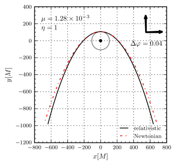
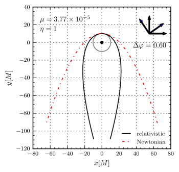
Figure 2: Trajectories followed by the FNC domain for $\eta=1$ encounters. Positions are given in units of black hole mass $M$. FNC domain motion for $\mu=1.28\times 10^{-3}$ is on the left and $\mu=3.77\times 10^{-5}$ is on the right. Relativistic precession of the frame through an angle $\Delta\varphi$ is indicated in the upper right corner (more pronounced for the $R_{p}\simeq 10M$ case). For reference the Newtonian parabolic orbit with the same pericentric distance is shown as the dashed curve.

III.1 Stellar model

The initial white dwarf is modeled as a nonrotating polytrope. The Lane-Emden equation with polytropic index $n=3/2$ provides initial density and pressure profiles, which are then mapped onto a three-dimensional Cartesian grid. The adiabatic index is taken to be $\gamma=5/3$, making the star neutrally stable against convection. We choose a mass $M_{*}=0.64M_{\odot}$ and radius $R_{*}=8.62\times 10^{8}$ cm, from which follows the remaining stellar properties. These properties are assembled in Table 1. They include the central density $\rho_{c}$, central pressure $p_{c}$, and stellar total energy $E_{\text{tot}}=-(3/7)\,GM_{*}^{2}/R_{*}=-E_{\text{int}}=\tfrac{1}{2}E_{g}$. We also calculate the moment of inertia $I_{*}=\tfrac{1}{3}\int x_{i}x_{i}\rho\,d^{3}x$ and the estimated break-up angular momentum $L_{*}=\sqrt{GM_{*}^{3}R_{*}}$. The fundamental radial pulsation period is given by $\tau_{0}=2\pi\sqrt{R_{*}^{3}/(\alpha M_{*})}$, where $\alpha=2.712$ results from our choice of $n=3/2$ and $\gamma=5/3$ cox1980 . A cold, degenerate white dwarf equation of state is not used, though we note the central density $\rho_{c}\sim 3\times 10^{6}$ g cm^-3 implies relativistic degeneracy would play a role. The size of the dimensionless gravitational potential ($\simeq 10^{-4}$) determines the accuracy of our formalism (Sec. II.4).

We investigate white dwarf–black hole encounters using three different mass ratios $\mu\equiv M_{*}/M$: $1.28\times 10^{-3}$, $4.21\times 10^{-4}$, and $3.77\times 10^{-5}$, corresponding to IMBH masses of $M=500\,M_{\odot}$, $M=1.52\times 10^{3}\,M_{\odot}$, and $M=1.70\times 10^{4}\,M_{\odot}$, respectively. The code uses black hole mass $M$ as the fundamental unit of mass, length, and time. The stellar parameters, when written in terms of $M$, therefore are functions of $\mu$. Their values are gathered in Table 2.

III.2 Orbits

The duration of each simulation is set equal to $10\,\tau_{0}$, with the star reaching pericenter at $\tau=0$. At pericenter $r=R_{p}$ the radial phase is $\chi=0$. The starting separation $R_{i}$ is chosen, which determines $\chi_{i}$ and the azimuthal angle $\phi_{i}$. In the FNC frame, the black hole appears to swing about through an angle $\Psi(\tau)$. The initial orientation of the frame can be freely chosen. The geodesic equations and the Eq. (24) for $\Psi$ are integrated. In the black hole frame the FNC frame vectors precess by an angle $\varphi$ that is the difference between $\phi$ and $\Psi$. These orbital parameters and the cumulative frame precession $\Delta\varphi$ are summarized in Table 3.

Figure 2 plots trajectories (as seen in the black hole frame in Schwarzschild coordinates) of the FNC frame center for a pair of $\eta=1$ encounters. Relativistic apsidal advance and frame precession are evident in passing both the $M=500M_{\odot}$ (left) and $17,000M_{\odot}$ (right) black holes, though both effects are more pronounced in the latter case. Plotted for comparison is the Newtonian parabolic orbit with the same pericentric distance.

III.3 Hydrodynamic parameters, resolution, and runtimes

The PPMLR hydro method (see Appendix A), like most grid-based schemes, requires that some tenuous atmosphere surround the star. The initial density $\rho_{\rm{atm}}$ and pressure $p_{\rm{atm}}$ are set low enough to not affect the dynamics of the star. To ensure this, we choose the atmospheric density to be $\rho_{\rm{atm}}=\rho_{c}\times 10^{-15}$. To set the pressure, we first assume a value for the initial atmospheric sound speed, taking it to be equal to the virial velocity at $r=2R_{*}$: $c_{\rm{atm}}^{2}=M_{*}/(2R_{*})$. The atmospheric pressure is then set equal to $p_{\rm{atm}}=c_{\rm{atm}}^{2}\rho_{\rm{atm}}/\gamma$.

It is also useful in the hydrodynamic scheme to set minimum values for the density and pressure ($\rho_{\rm{floor}},p_{\rm{floor}}$) that cannot be breached. Such a floor sometimes proves necessary, as a strong shock wave encountering another large discontinuity in density might otherwise yield a zone with negative density or pressure. The floor density and pressure can be set quite low. We take $\rho_{\rm{floor}}=\rho_{c}\times 10^{-25}$ and $p_{\rm{floor}}=c_{\rm{atm}}^{2}\rho_{\rm{floor}}/\gamma.$

While an elongated domain might be used, all of our simulations involved a box with equal side lengths and an evenly-spaced Cartesian grid. We tested the degree of convergence of all of our results by using meshes with $128^{3}$, $256^{3}$, or $512^{3}$ total numbers of zones. The length of the side of the computational domain was set to $L=4R_{*}$ for stellar equilibrium tests and weak ($\eta=4-6$) encounters. For stronger or disruptive encounters the domain is taken to be larger, with $L=8R_{*}$. Resolution depends primarily on the number of zones across the radius of the initial star. We refer to the different resolutions by $\Delta_{A}$, $\Delta_{B}$, and $\Delta_{C}$, with $\Delta_{A}=R_{*}/32$, $\Delta_{B}=R_{*}/64$, $\Delta_{C}=R_{*}/128$. Also, zero-gradient outflow boundary conditions are used on the domain surface.

The domain is split into slabs for computing on a cluster. For simplicity we took the slabs to be one-zone thick sheets and allocated one cluster core per sheet. Thus the number of cores is locked to the number of zones in one direction. Our highest resolution runs used 512 processors. At this resolution simulations lasting ten dynamical times required between 88 and 127 hours of wall-clock time.

III.4 Equilibrium configurations and tests of hydro plus gravity

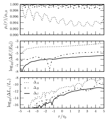
Figure 3: Tests of hydrostatic equilibrium with a polytropic star having $n=3/2$ and $\gamma=5/3$. In the top panel we plot the central density $\rho_{c}(\tau)$ as a function of time, normalized by its initial value. The time $\tau$ on the horizontal axis (shared by all three panels) is given in units of the fundamental radial pulsation period $\tau_{0}$. Low amplitude pulsations are evident at exactly the $F$-mode period, which last $>10$ periods. Models with three different resolutions, $\Delta_{A}$, $\Delta_{B}$, $\Delta_{C}$ (see text) are compared. Convergence to equilibrium is evident. Small secular drift in the central density occurs, a result of weak spurious entropy generation in the hydro code. The second panel plots fractional change in total energy $E_{\rm tot}(\tau)$. Higher resolution models conserve energy to $\lesssim 10^{-5}$. The bottom panel plots the change in total spin angular momentum $L_{\rm tot}(\tau)$ scaled relative to a dimensional estimate of break-up angular momentum $L_{*}$.

An important test is how close to exact stellar equilibrium can three-dimensional simulations be held. Equilibrium models serve as a control, especially for weak tidal encounters. The Lane-Emden equation is integrated with a fine one-dimensional mesh. The resulting hydrodynamic radial profiles are mapped onto the three-dimensional Cartesian mesh of chosen resolution. The Poisson solver (see Appendix A) is then called to find the self-gravitational potential in the three-dimensional domain.

The resulting stellar model is found to be close to but not exactly in equilibrium. The top panel of Fig. 3 reveals a small fractional oscillation and drift in the central density. Three main sources of error contribute to breaking equilibrium. First, there is discretization error in mapping the well-resolved one-dimensional Lane-Emden radial profiles onto a three-dimensional Cartesian grid. Second, there are inaccuracies in the gravitational field obtained with the Poisson solver. These two effects combine to place the initial star slightly out of hydrostatic equilibrium and in response the star oscillates, primarily in the fundamental radial mode (Fig. 3). Third, there is a weak spurious generation of entropy within the star, a byproduct of the PPM algorithm (and many other hydro schemes bale2002 ). In PPM, any gradient in density and pressure, even when balanced by gravitational acceleration in hydrostatic equilibrium, is viewed by the method as a discontinuity, or small shock. Small secular increases in entropy occur, leading to slight expansion of the star and decrease in central density. As Fig. 3 shows, at low resolution the effect is an average decrease in density of $\sim 0.5$ % over five to ten dynamical times.

Both of these effects are reduced with higher resolution. In these tests we used domains with $128^{3}$, $256^{3}$, and $512^{3}$ zones. In each case the domain length was four times the radius of the star, $L=4R_{*}$, and so the three resolutions considered had 32, 64, and 128 zones per $R_{*}$. Based on this test, we take the lowest resolution of interest to be $\Delta_{A}$, with our best results requiring resolutions of $\Delta_{B}$ and $\Delta_{C}$. At the higher resolutions we hold total energy conservation to $\lesssim 10^{-5}$ and the equilibrium models have effectively no tendency to generate spurious angular momentum.

During a tidal encounter, however, a star will be set into nonradial (and radial) oscillations. The amplitude and persistence of these oscillations is an important result to be derived from the numerical simulations. The tests in this section show that stellar pulsations are well maintained by our code even at modest resolution. The radial mode is seen to damp in amplitude over time but with $Q\simeq 40$.

IV Hydrodynamic features and mass stripping in weak tidal encounters

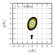
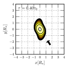
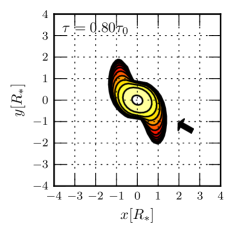
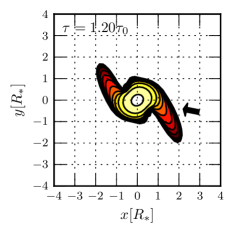
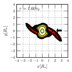
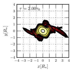
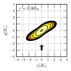
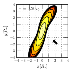
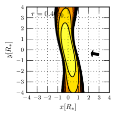
Figure 4: Density contour plots of an $\eta=3$ encounter with $\mu=3.77\times 10^{-5}$. Positions are in units of $R_{*}$. The contour lines are of $\log_{10}\rho$, ranging from $-8$ to $-2$ in steps of $0.5$ (as seen in the equatorial plane). Besides the Newtonian quadrupole, the octupole tidal term and (orbital) relativistic correction to the quadrupole term have been included in the calculation.

Figure 5: Density contour plots of an $\eta=1$ encounter with $\mu=3.77\times 10^{-5}$. Positions are in units of $R_{*}$. The simulation begins at $\tau=-5\,\tau_{0}$, reaches pericenter at $\tau=0$, and ends at $\tau=5\,\tau_{0}$. The contour lines are given for $\log_{10}\rho$ from $-8$ to $-2$ in steps of $0.5$. Note slight deflection of the CM in this and preceding figure.

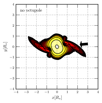
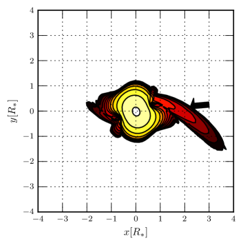
Figure 6: Contour plots of density of the star in the x-y plane at $\tau=1.7\,\tau_{0}$ for an $\eta=3$ encounter with $\mu=1.28\times 10^{-3}$. Positions are in units of $R_{*}$. The contour lines are given for $\log_{10}\rho$ from $-11$ to $-5$ in steps of 0.5. Comparison is made between a simulation with only the quadrupole ($l=2$) tidal terms (left) and one with both the quadrupole and octupole ($l=3$) tidal terms included (right). Resolution of these simulations is $\Delta_{B}$. The effect of the octupole tidal terms in driving a deflection of the CM is evident in the asymmetry of the tidal lobes.

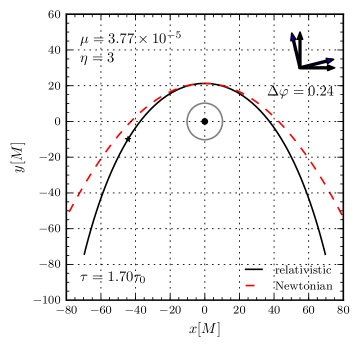
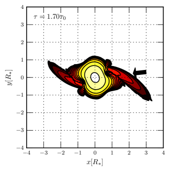
Figure 7: An $\eta=3$ encounter with more extreme mass ratio $\mu=3.77\times 10^{-5}$. Results shown at time $\tau=1.7\,\tau_{0}$. On the left, position of the frame center is marked on the orbit. On the right are shown density contours in the x-y plane. The contour lines are given for $\log_{10}\rho$ from $-8$ to $-2$ in steps of $0.5$. The quadrupole and octupole tidal terms have been included. For this more extreme mass ratio, the effects of the octupole tide are less pronounced (compare to Fig. 6).

In this section we consider some of the qualitative hydrodynamic features that are seen in tidal encounters, focusing especially on our inclusion of a higher-order tidal moment. In addition, we calculate and show the amount of mass loss that occurs as a function of parameter $\eta$ for weak tidal encounters between a white dwarf and an IMBH.

IV.1 Octupole tidal term

In general our simulations could include all of the tidal acceleration terms identified as potentially significant in Sec. II. However, it is useful to turn various terms on or off and compare simulations to see the resulting effects. One result of doing so is that we find that our mass ratios are too small to make inclusion of the $l=4$ tide worthwhile. Consequently we have not included $l=4$ in any of the results in this paper. The same is not true of the octupole tide ($l=3$), which generates interesting physical effects.

In Figs. 5 and 5 we consider encounters at our most extreme mass ratio ($\mu=3.77\times 10^{-5}$) and with encounter strengths $\eta=3$ and $\eta=1$, respectively. In these simulations we have included the full tidal field. With $\eta=3$ the star is tidally disturbed with a small fraction of mass stripped from the star, as can be seen at a sequence of times in Fig. 5. In contrast, the star is fully tidally disrupted when $\eta=1$, as seen in Fig. 5. Similar but not identical results from high-resolution mesh-based calculations can be found in Refs. khok1993 ; khok1993strong ; frol1994 . The primary difference is our inclusion of the octupole tidal term, whose effect shows up in the asymmetry of the tidal lobes in Fig. 5 and the deflection of the CM that is also evident in both Fig. 5 and Fig. 5.

Figure 6 even more clearly shows the effects of the octupole tide. In this case we plot an $\eta=3$ encounter with less extreme mass ratio $\mu=1.28\times 10^{-3}$. The full tidal field is incorporated in the simulation shown in the right panel, while the left panel shows the same simulation except for switching off the octupole tide. The arrow represents the direction from the black hole to the origin of the FNC frame. For contrast Fig. 7 shows on the right side an $\eta=3$ encounter at the same dynamical time but from a simulation with our most extreme mass ratio. The asymmetry is still present but much less pronounced, as reference to Fig. 1 and the analysis of Section II.5 would suggest.

IV.2 Mass loss in weak tidal encounters

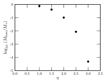
Figure 8: Fraction of mass stripped from white dwarf as a function of $\eta$ for weak tidal encounters. In each simulation the mass ratio was fixed at $\mu=1.28\times 10^{-3}$ and we plot the fraction of mass lost from the domain at $\tau=5\,\tau_{0}$ (the end of the simulations). The fraction of mass lost for $\eta=4$ was also computed and found to be $\simeq 10^{-10}$ (off scale).

Weak tidal encounters may result as stars diffuse into the loss cone of a SMBH or IMBH. Successive passages may heat the star and the induced oscillations may be resonant with the orbit rath2005 . Gravitational bremsstrahlung may be important as well for compact systems. The combination of these effects spurs a reduction in $\eta$ with each passage.

Another important effect of weak encounters is partial mass stripping. In the absence of competing effects, any mass loss will be reflected in the star having a lower average central density and larger average radius during the next encounter. This effect in turn shifts $\eta$ to a lower value and enhances the likelihood of disruption krol2011 .

We have calculated the amount of mass loss in a set of weak tidal encounters. In Fig. 8, the fractional amount of mass stripped from the star and lost from the computational domain is given for a range of encounter parameters from $\eta=1$ through $\eta=3$. (The $\eta=4$ case was computed as well but the measured mass loss fraction of $\simeq 10^{-10}$ may be low enough to be affected by the “atmosphere” we are forced to add to the hydrodynamic simulations.) The $\eta=1$ case involved complete disruption. In each case we held the mass ratio fixed at $\mu=1.28\times 10^{-3}$.

For $\eta\gtrsim 2$ ($R_{p}\gtrsim 1.6\,R_{t}$) the amount of mass loss is small enough that multiple passages with partial stripping should occur. If the star were not heated (but see Sec. V), then the response of the mean radius would be determined by $\delta R_{*}/R_{*}=-(1/3)\delta M_{*}/M_{*}$ and $\delta\eta/\eta=\delta M_{*}/M_{*}$. The $1.0$ % mass loss at $\eta=2.5$, for example, would induce a radius increase of only $0.3$ % and a drop in $\eta$ of 1 %. At $\eta=2$ however, the mass loss is $10$ % and the mean radius increase would be $3$ %, leading to a 10 % drop in $\eta$. As we will show in the next section, shock heating is important as well and the effects of mass loss just set a lower bound on effective reduction of $\eta$.

V Tidal energy deposition, relativistic effects, and capture

In this section we discuss the transfer of energy into the star that occurs as a result of tidal interaction. This topic has been addressed previously (see e.g., pres1977 ; cart1985 ; lee1986 ; khok1993 ). We consider the subject again for several reasons. First, our FNC system is tailored to follow small relative motions with respect to the initial timelike geodesic. Second, the FNC expansion we use retains higher-order moments and orbital relativistic effects. Finally, we are able to apply relatively high resolution ($512^{3}$) and assess convergence of our numerical results.

The equation of motion (69) of the fluid in the FNC frame is nearly Newtonian. As such we can carry over much of the standard understanding of tidal heating cart1985 with only minimal modification. If we contract Eqs. (69) and (70) with $v^{i}$, use the continuity equation and first law of thermodynamics, we obtain the equation of energy conservation of the star (as seen in the FNC frame)

$$\frac{\partial}{\partial\tau}\left(\rho\Pi+\tfrac{1}{2}\rho v^{2}\right) + \frac{\partial}{\partial x^{k}}\left[\rho v^{k}\left(\Pi+\frac{p}{\rho}+\tfrac{1}{2}v^{2}\right)\right]+\rho v^{i}\frac{\partial\Phi_{*}}{\partial x^{i}}$$ (71)

$$\quad=-\rho v^{i}\frac{\partial\Phi_{\text{tidal}}}{\partial x^{i}}-\rho v^{i}\frac{\partial A_{i}}{\partial\tau}.$$

Integrating over a volume encompassing all of the material, we can define the internal energy $U_{*}=\int\rho\Pi\,d^{3}x$, self-gravitational energy $\Omega_{*}=\tfrac{1}{2}\int\rho\Phi_{*}\,d^{3}x$, and kinetic energy $T_{*}=\tfrac{1}{2}\int\rho v^{2}\,d^{3}x$. The equation of energy conservation of the star is then

$$\frac{dE_{*}}{d\tau}=-\int\rho v^{i}\frac{\partial\Phi_{\text{tidal}}}{\partial x^{i}}\,d^{3}x-\int\rho v^{i}\frac{\partial A_{i}}{\partial\tau}\,d^{3}x,$$ (72)

where the total energy $E_{*}=U_{*}+\Omega_{*}+T_{*}$ would be conserved in the absence of tides. We have assumed that the fluid remains adiabatic (no radiative cooling) and that no mass or energy fluxes through a sufficiently large bounding surface.

To gain a physical picture, imagine dropping the gravitomagnetic potential $A_{i}$ (61) and retaining only Newtonian terms in the tidal potential $\Phi_{\rm tidal}$ (60). Then the tidal energy transfer cart1985 would reduce to

$$\frac{dE_{*}}{d\tau}=-\tfrac{1}{2}C_{ij}^{(0)}\,\dot{I}_{ij}-\tfrac{1}{6}C_{ijk}^{(0)}\,\dot{I}_{ijk}+\cdots,$$ (73)

where $I_{ij}=\int\rho x_{i}x_{j}d^{3}x$ and $I_{ijk}=\int\rho x_{i}x_{j}x_{k}d^{3}x$ are the second and third mass moments, dot refers to the time derivative, and of course only the trace-free parts of $I_{ij}$ and $I_{ijk}$ contribute. While our code calculates all of the moments and relativistic corrections we enumerated in Sec. II, the quadrupole tide still dominates the energy transfer.

V.1 Total energy deposition and comparison with linear theory

A series of simulations were run with a fixed mass ratio of $\mu=1.28\times 10^{-3}$ but with varying encounter parameters ($\eta=1$ through $\eta=6$) and at three different resolutions. In each case we measured the final total energy of the configuration as seen in the FNC frame and compared it to the initial energy of the inbound star. The tidal field was seen to do work on the star and the gain in energy is depicted in Fig. 9.

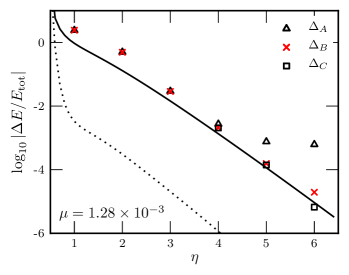
Figure 9: Measured energy deposition versus encounter parameter $\eta$ and comparison with linear theory. Each simulation was made with $\mu=1.28\times 10^{-3}$. The points indicate measured fractional increases in the total energy of the star at the end of each simulation. Results are given at three different resolutions for each $\eta$. The measured energies are numerically well converged for $\eta=1$ through $\eta=4$, and probably $\eta=5$ as well. Our range of resolution is not adequate to measure the deposited energy for $\eta=6$, which is at the level of $10^{-5}$ of the initial stellar energy. The solid curve gives the prediction of linear theory for the contributions of the quadrupole ($l=2$) and octupole tides and the nonradial oscillations they induce. The dotted curve is the prediction for the octupole ($l=3$) tide alone, which is two orders of magnitude smaller than the quadrupole at this mass ratio.

Table 4: Energy deposited into the star or debris as a function of tidal parameter $\eta$. The second column gives the fractional increase in the energy of the star relative to the magnitude of the star’s initial total energy. The third column gives the expected fractional increase in energy based on linear theory of excitation of nonradial modes. The fourth column gives the difference, which is a fractional excess energy deposition. The fifth column estimates the amount of the excess energy that might be attributed to shock heating and the sixth column estimates the amount of the excess that could be explained by excitation of the fundamental radial mode. Each encounter was simulated with a mass ratio of $\mu=1.28\times 10^{-3}$. Tabulated numbers in column two were drawn from our highest resolution runs.

$\eta$	$\frac{\Delta E_{\rm dep}}{|E_{\text{tot}}|}$	$\frac{\Delta E_{\rm lin}}{|E_{\text{tot}}|}$	$\frac{\Delta E_{\rm ex}}{|E_{\text{tot}}|}$	$\frac{\Delta E_{\rm shock}}{|E_{\text{tot}}|}$	$\frac{\Delta E_{\rm rad}}{|E_{\text{tot}}|}$
1	2.41	9.39e-01	1.48
2	4.89e-01	1.30e-01	3.59e-01	3.3e-01	8.9e-02
3	2.89e-02	1.44e-02	1.45e-02	2.4e-02	1.6e-03
4	2.11e-03	1.34e-03	7.68e-03	2.0e-03	1.4e-05
5	1.50e-04	1.15e-04	3.49e-05
6	1.16e-05	9.23e-06	2.40e-06

The energy gain is also tabulated in Table 4, but expressed as a ratio to the magnitude of the total energy $E_{\text{tot}}=-(3/7)\,GM_{*}^{2}/R_{*}$ of the initial star. We see that for $\eta=1$ the star has come apart. Progressively less energy is deposited for weaker encounters. By comparing simulations made at three different resolutions it is apparent that the results for $\eta=1$ through $\eta=5$ have converged. The result for $\eta=6$ is less well known. In any event, we appear able to determine accurately fractional energy depositions as small as $10^{-4}$.

Energy observed in the simulations to be deposited onto the star can be compared to the predictions of linear theory. Press and Teukolsky pres1977 and Lee and Ostriker lee1986 calculated the amount of energy that a time-dependent linear perturbation in the gravitational potential would induce via the excitation of nonradial modes. The interaction is decomposed into spherical harmonics, and each tidal multipole will excite the corresponding lowest frequency nonradial $l$ mode. The total energy deposited is a sum over each $l$ mode contribution and is given by

$$\Delta E_{\text{lin}}=\left(\frac{GM_{*}^{2}}{R_{*}}\right)\left(\frac{M}{M_{*}}\right)^{2}\sum_{l=2,3,...}\left(\frac{R_{*}}{R_{p}}\right)^{2l+2}T_{l}(\eta),$$ (74)

where the key to the theory is calculating the dimensionless functions $T_{l}(\eta)$ pres1977 , which depend on $\eta$ and also the polytropic index $n$. We use the results for $T_{l}$ obtained previously lee1986 ; port1993 for an $n=3/2$ polytrope.

The mass ratio (taken to be $\mu=1.28\times 10^{-3}$ in this section) affects the relative magnitude of the $l=2$ and $l=3$ excitations, as reference to (74) makes clear. In Fig. 9 we plot the curves for both the $l=2$ and $l=3$ contributions to $\Delta E_{\text{lin}}$. The linear contribution of the octupole tide is two orders of magnitude below that of the quadrupole.

We see a clear convergence with linear theory in the limit of weak encounters (up to $\eta=5$). As the strength of the encounter grows the energy actually deposited is seen to exceed the predictions of linear theory. This excess in energy deposition appears to be real (based on numerical convergence) and confirms results discovered previously khok1993 . As Table 4 indicates, the excess can be as much as 50% to 75% of the total. The result has important implications for predictions of the cross section for tidal capture of stars.

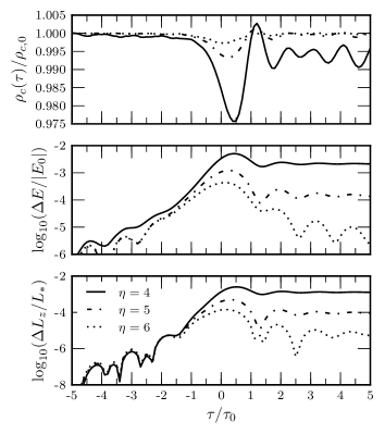
Figure 10: Weak tidal encounters. Top panel shows fractional changes in central density for $\eta=4$, $\eta=5$, and $\eta=6$ encounters. Mid panel shows (normalized) energy deposited for each encounter. Bottom panel displays (normalized) spin angular momentum deposited for each encounter. The mass ratio is $1.28\times 10^{-3}$. Each curve is drawn from the highest resolution ($\Delta_{C}$) simulations.

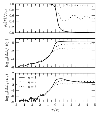
Figure 11: Partial and complete disruptions. Same as previous figure except displaying results for $\eta=1$, $\eta=2$, and $\eta=3$ encounters. The star disrupts completely when $\eta=1$ as seen by behavior of central density. Energy deposition continues to rise with the strength of the encounter, while angular momentum deposition saturates. The mass ratio is $1.28\times 10^{-3}$. Results are drawn from highest resolution simulations.

V.2 Shock heating and the energy excess

The time dependence of the central density of the white dwarf provides clues on where the excess energy resides. In Fig. 10 and 11 the top panels show $\rho_{c}(t)$ normalized by the initial central density of the star. Figure 10 shows the behavior for weak tidal encounters ($\eta=4$, $\eta=5$, and $\eta=6$) and Fig. 11 displays stronger encounters ($\eta=1$, $\eta=2$, and $\eta=3$). All models were computed with $\mu=1.28\times 10^{-3}$. Complete disruption is evident for $\eta=1$. For weaker encounters the central density typically decreases to a new lower average value and oscillates. The average normalized central density, post-encounter, is (1) $\rho_{c}^{\prime}/\rho_{c}\simeq 0.5$ for $\eta=2$, (2) $\rho_{c}^{\prime}/\rho_{c}\simeq 0.93$ for $\eta=3$, and (3) $\rho_{c}^{\prime}/\rho_{c}\simeq 0.995$ for $\eta=4$.

For a polytropic model, a reduction in the central density can arise either by reducing the mass of the star or by increasing $K=p/\rho^{1+1/n}$. As we have already seen, weak encounters involve some loss of mass. Furthermore, as our sequence of contour plots indicates, weakly disturbed stars are affected by formation of shocks in the outer layers. The heating is not uniform but we can get an approximate sense of the effects by assuming it is. For the nonce we assume that $K\rightarrow K^{\prime}>K$ following the encounter. For a $n=3/2$ polytrope, the following scaling laws hold

$$K\sim M_{*}^{2/3}\,\rho_{c}^{-1/3},\quad R_{*}\sim M_{*}^{1/3}\,\rho_{c}^{-1/3},\quad|E_{\text{tot}}|\sim M_{*}^{5/3}\,\rho_{c}^{1/3}.$$ (75)

We treat the mass loss and change in central density as observables that indicate a new approximate polytropic state. Using the scalings, we can estimate that the change in total energy of the star would follow

$$\Delta E\simeq|E_{\text{tot}}|\left[1-\left(\frac{M_{*}^{\prime}}{M_{*}}\right)^{5/3}\left(\frac{\rho_{c}^{\prime}}{\rho_{c}}\right)^{1/3}\right].$$ (76)

Except for the case $\eta=2$ where 10% of the mass is lost, the resulting changes in energy are mostly the result of shock heating. Using the values obtained from Figs.  8, 10, and 11, we estimate the effects of (assumed) uniform heating and list the results in the fifth column of Table 4. The correspondence with the fractional excess energy gain in column four is suggestive that shock heating provides the sink for most of the excess.

V.3 Radial mode excitation

After weak tidal encounters with the black hole, the white dwarf is observed to oscillate not only in the quadrupole ($l=2$, $m=\pm 2$) $f$ modes but also in the fundamental radial $F$ mode. This can best be seen by the oscillations in central density in Figs. 10 and 11 for the $\eta=3$ and $\eta=4$ encounters. In those two cases the observed oscillations match the period of the linear radial $F$ mode almost exactly.

The excitation of the radial mode was noted by Khoklov et al. (1993) khok1993 ; khok1993strong . Excitation of this mode by a tidal field is not possible at linear order. Khoklov et al. attributed it to a nonlinearity in the post-encounter hydrodynamics. They further suggested that it might be a locus of some of the excess energy gain.

To examine this idea, we simulated a set of dynamical stellar models that were deliberately set into radial oscillation. In these tests no tidal field was included. By varying the amplitude of the radial oscillation we sought to correlate the increase in energy in the star with the amplitude of oscillation in the central density. The observed oscillations in the central density that occur in our tidal encounters could then be used to estimate the amount of energy in the radial mode.

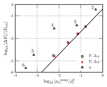
Figure 12: Excitation of the fundamental radial mode. We compare radial pulsation models with those of tidal encounters for $\eta=2-6$ and for mass ratio $\mu=1.28\times 10^{-3}$. Squares and crosses indicate results for radial oscillation simulations, measuring the added energy of the star versus amplitude of the oscillation in the central density. The line indicates a quadratic dependence. Individual triangles are points constructed from tidal encounter simulations, plotting the excess deposited energy versus observed amplitude of the central density oscillation. For weak encounters the observed energy excess is an order of magnitude or two higher than can be explained by excitation of the fundamental radial mode. Energy in the radial mode can be 11% to 25% of the excess in encounters with $\eta=3$ and $\eta=2$.

We generate radially pulsating models by introducing a homologous scaling of the Lane-Emden density profile as an initial condition. Consider a homologous mapping of the star that takes the original radius $R_{*}$ to $R_{*}^{\prime}=R_{*}/\lambda$ via scaling parameter $\lambda$. Assume that the equilibrium stellar profile is $\rho(r)$. Map the original density profile to a new one using

$$\bar{\rho}(r)=\lambda^{3}\rho(\lambda r).$$ (77)

With this scaling the mass is unaffected by the transformation. Then we assume that $K$ does not scale and calculate the altered pressure profile from the new density taking the polytropic index fixed also. The scaled density is used to calculate a new gravitational potential, which no longer provides hydrostatic equilibrium. Technically, the initial radial displacement is linear, which would not match the shape of the fundamental radial mode amplitude. Accordingly, we might expect a set of radial overtones to be excited. Practically, though, most of the excitation is observed to be in the $F$ mode.

We compute models with parameter range $\lambda=[0.9,0.95,0.98,0.995,1.005,1.02]$. We compare the change in total energy between the radially pulsating models and the equilibrium model, $\Delta E^{\lambda}_{\rm tot}-\Delta E^{\lambda=0}_{\rm tot}$, with the observed amplitude of oscillation in the central density. The resulting points form an approximately quadratic power-law relationship, as can be seen in Fig. 12.

To compare these radially pulsating models to the tidal encounters, we read off the amplitude of central density oscillations from Figs. 10 and 11 for different $\eta$. These oscillation amplitudes and the observed tidal excess energy for the same $\eta$ are used to plot points in Fig. 12 also. They are marked in the figure to indicate their associated value of $\eta$. In all tidal encounter cases the excess energy is greater than can be explained by energy in the excitation of the radial mode, though for $\eta=2$ and $\eta=3$ the radial mode may be a non-negligible contributor at the level of 25% to 11%, respectively. For weaker encounters the radial mode is as much as two orders of magnitude smaller. Some numerical values are compared in Table 4.

V.4 Relativistic effects on energy deposition

Another way to see the excess in energy deposited on the star is to plot its value normalized to the value expected from linear theory. Figure 13 shows the data for weak encounters in this fashion, but does so for all three mass ratios. The plot shows clearly how the excess energy grows with increasing tidal encounter strength and yet approaches the linear result nicely for the weakest encounters.

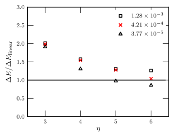
Figure 13: Energy deposition normalized to expected values from linear theory. Three mass ratios were examined. All of the simulations were made at highest resolution, $\Delta_{C}$. Growth in energy transfer with increasing tidal strength is evident. Also evident is the effect of relativistic motion and relativistic tidal corrections in the most extreme mass ratio case (triangles). A slight suppression in energy transfer appears at $\eta=3$, $\eta=4$, and $\eta=5$ for $\mu=3.77\times 10^{-5}$ that differs from the mutually consistent values seen at less extreme mass ratios.

More importantly, this plot shows the presence of relativistic effects on the energy transfer. All of these simulations were done at our highest resolution, $512^{3}$. The only variables were $\eta$ and $\mu$. As we discussed previously, the $\eta=6$ results are not numerically converged but the results for $\eta=3$ through $\eta=5$ are. For the most extreme mass ratio (triangles in the plot), the star passes much closer to the black hole and the effects of relativistic motion and relativistic corrections in the tidal field will be more pronounced. We observe a slight suppression in the energy transfer for $\eta=3$ through $\eta=5$. Simulations run at several resolutions indicate the effect is real. Notice the level of consistency in the energy transfer that occurs for the other two, less extreme mass ratios.

An explanation for the suppression likely can be found in a modification of the linear theory. As Press and Teukolsky pres1977 show, the overlap integral for the tidal interaction at each mode $nlm$ involves a product between two terms, $Q_{nl}$ (which depends upon the normal mode amplitudes) and $K_{nlm}$ (which depends upon the time dependence of the amplitude and phase of the $lm$ part of the tidal field). In the FNC frame (with approximately Newtonian self-gravity and a weak tidal field), the integrals for $Q_{nl}$ are indifferent to whether the orbital motion is relativistic or not. The same is not true of $K_{nlm}$ [Press and Teukolsky’s Eq. (39)]. For example with $l=2$, the tidal amplitude will not only vary as $r(t)^{-3}$ but will be corrected by an (orbital) 1PN term that behaves as $r(t)^{-5}$ (II.3). Furthermore, the relativistic shape of the orbit will be important and the motion of the black hole in the FNC frame requires that the azimuthal angle $\phi(t)$ in their equation be replaced by $\Psi(t)$. In effect, $T_{l}(\eta)$ has to be replaced by a function $T_{l}(\eta,\Phi_{p})$ of $\eta$ and a measure of the depth of the relativistic potential, $\Phi_{p}=M/R_{p}$.

V.5 Capture orbits: effects of tides and gravitational bremsstrahlung

The energy transferred into the star by the tides comes at the expense of orbital energy. If we assume the inbound white dwarf has zero total orbital energy ($\tilde{E}=1$ in the relativistic sense), the orbital energy after the encounter becomes $E_{\text{orb}}=-\Delta E$ and can be used to estimate the semi-major axis $a=-M_{*}M/2E_{\text{orb}}$ of the initial capture orbit. For compact systems, and especially for higher mass black holes, the effect of gravitational wave bremsstrahlung should be included. The orbital energy is then $E_{\text{orb}}=-\Delta E_{\text{tidal}}-\Delta E_{GW}$.

To calculate the gravitational bremsstrahlung, we approximate the orbital motion as Newtonian and first use the classic result pete1964 for the rate of energy loss averaged over one period of a bound orbit

$$\left<\frac{dE}{dt}\right>=\frac{32}{5}\frac{G^{4}(M+M_{*})M^{2}M_{*}^{2}}{c^{5}a^{5}}f(e),$$ (78)

where the eccentricity $e$ determines

$$f(e)=\left(1-e^{2}\right)^{-7/2}\left(1+\frac{73}{24}e^{2}+\frac{37}{96}e^{4}\right).$$ (79)

Multiplying this luminosity by the orbital period $T=2\pi a^{3/2}/[G(M+M_{*})]^{1/2}$ yields the amount of energy radiated in one period

$$\Delta E_{GW}=\frac{64\pi}{5}\frac{G^{7/2}(M+M_{*})^{1/2}M^{2}M_{*}^{2}}{c^{5}}f(e)a^{-7/2}.$$ (80)

To get the burst associated with a parabolic orbit, we replace $a$ in the above formula with pericentric distance $R_{p}=a(1-e)$ and then take the limit as $e\rightarrow 1$

$$\Delta E_{GW}=\frac{85\pi\sqrt{2}}{24}\frac{G^{7/2}}{c^{5}}\frac{(M+M_{*})^{1/2}M^{2}M_{*}^{2}}{R_{p}^{7/2}}.$$ (81)

Table 5: Capture orbits from the combined effects of tidal energy transfer and gravitational bremsstrahlung. A range of $\eta$ for weak encounters in which the white dwarf survives is considered. Three mass ratios $\mu$ are examined. Tidal energy transfer and gravitational wave loss are separately listed. Energies are compared to the scale of kinetic energy $T_{p}=MM_{*}/R_{p}$ at pericenter. The importance of gravitational bremsstrahlung rises with increasing black hole mass. The resulting capture orbits are given in terms of the ratio $R_{\text{max}}/R_{p}$ between apocentric and pericentric distances.

$\mu$	$\eta$	$\frac{\Delta E_{\rm GW}}{T_{p}}$	$\frac{\Delta E_{\text{tidal}}}{T_{p}}$	$\frac{R_{\rm max}}{R_{p}}$
$1.28\times 10^{-3}$	2	5.30e-08	3.92e-03	2.54e+02
-	3	2.70e-08	3.04e-04	3.29e+03
-	4	1.67e-08	2.69e-05	3.72e+04
-	5	1.15e-08	2.21e-06	4.50e+05
$4.21\times 10^{-4}$	2	1.11e-07	1.90e-03	5.25e+02
-	3	5.65e-08	1.43e-04	6.99e+03
-	4	3.50e-08	1.26e-05	7.94e+04
-	5	2.41e-08	1.03e-06	9.48e+05
$3.77\times 10^{-5}$	2	5.53e-07	4.59e-04	2.18e+03
-	3	2.83e-07	2.75e-05	3.60e+04
-	4	1.75e-07	2.12e-06	4.35e+05
-	5	1.20e-07	1.58e-07	3.60e+06

We list results for tidal capture of white dwarfs in Table 5. There we tally the amount of tidal energy transfer observed in the simulations for different mass ratios $\mu$ and encounter strengths $\eta$ (for those cases in which the star survives). Also given is the amount of gravitational wave energy loss during the encounter. (There is also gravitational wave emission from the internal hydrodynamic motions of the star, but these can be shown to be orders of magnitude smaller.) Energies are given relative to the scale of kinetic energy of the star at pericenter, which is easily obtained from Table 3. The effect of the tides dominates but gravitational bremsstrahlung increases in importance for more massive black holes. Given the total energy loss from the orbit, the capture orbit can be described by the ratio $R_{\text{max}}/R_{p}=(1+e)/(1-e)$ between the apocentric and pericentric distances.

VI Angular momentum

A tidal encounter transfers not only energy but also angular momentum. Since the fluid equations are nearly Newtonian in the FNC frame, the standard analysis of self-gravitating fluids cart1985 provides an approximate physical picture. Let the spin tensor be

$$J_{ik}=\tfrac{1}{2}\int\rho(x_{i}v_{k}-v_{i}x_{k})d^{3}x,$$ (82)

and the first moment of the tidal force tensor be

$$F_{ik}=-\int\rho x_{i}\partial_{k}\Phi_{\text{tidal}}d^{3}x\simeq-I_{ij}C_{jk}^{(0)}.$$ (83)

The antisymmetric part of the tensor virial theorem expresses conservation of angular momentum and we find that the tidal field exerts a torque given by

$$\dot{J}_{ik}=-\tfrac{1}{2}\left(I_{ij}C_{jk}^{(0)}-I_{kj}C_{ji}^{(0)}\right)+\cdots.$$ (84)

A torque results whenever the bulge drawn up dynamically in $I_{ij}$ lags (or leads) the principal axis of the tidal field. Numerically we compute the action of the full tidal field, including higher order moments and (orbital) relativistic corrections. But the most important contributor to the torque remains the Newtonian part of the quadrupole tide.

In our models, the black hole appears to move (in the FNC frame) in the $x$-$y$ plane, which induces changes in the $z$ component of the white dwarf’s spin angular momentum, $L_{z}$. The bottom panels of Figs. 10 and 11 show the growth in $L_{z}$ (normalized to an estimate of breakup angular momentum) during tidal encounters of varying strength. The total amount of angular momentum deposited in the star varies over four orders of magnitude in models that range from $\eta=6$ to $\eta=1$. In several cases the spin overshoots before settling back nolt1982 , an effect of the black hole racing out more than 90 degrees ahead of the principal axis of the star.

VI.1 Center of mass deflection

The deposition of angular momentum has been seen in many past numerical studies. What is new in this paper is calculating the effects of the octupole tide, $C_{ijk}$. We can again get a physical picture by considering Newtonian behavior. Let the first moment of the mass distribution be $D_{k}=\int\rho\,x_{k}\,d^{3}x$. Then take the momentum equation (69), restrict it to Newtonian terms, and construct an equation of motion for $D_{k}$,

$$\ddot{D}_{k}=-C_{ki}^{(0)}D_{i}-\tfrac{1}{2}C_{kij}^{(0)}I_{ij}-\tfrac{1}{6}C_{kijl}^{(0)}I_{ijl}+\cdots.$$ (85)

If the octupole and other higher-order moments vanish, and if the star is initially centered on the frame $D_{k}=0$, then the CM has no tendency to move. If however the octupole tide is present, it couples to the second mass moment and drives an acceleration of the CM. Once the CM shifts the quadrupole tide plays a role also.

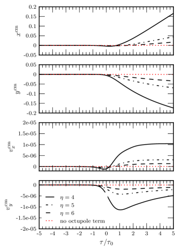
Figure 14: Deflection of the center of mass. Positions (top two panels) and velocities (bottom two panels) of the CM in simulations with $\eta=4,5,6$ and mass ratio $\mu=1.28\times 10^{-3}$. A simulation with no octupole tidal term is shown (dotted red line) for comparison. The resolution in each case was $512^{3}$.

Since our models include the octupole tide, we see its effect on CM motion. Some of these effects are apparent in the contour plots shown earlier in Figs. 5, 5, and 6, primarily in the asymmetry of the tidal lobes. More quantitatively, we compared simulations that included only the quadrupole ($l=2$) tide with ones that included both the quadrupole ($l=2$) and octupole ($l=3$) terms. In Fig. 14, the octupole tide can be seen to cause a deflection of the CM of the star away from the FNC origin (here we show actual shifts in position, not components of $D_{k}$). No deflection is seen in the quadrupole-only model. The size of the deflection can also be seen to depend upon the strength of the encounter. These small positional changes and velocities are well determined at our highest resolution.

VI.2 Orbital angular momentum change

Surprisingly (from a numerical standpoint) the CM position and velocity are determined well enough that we can compute from them the change in orbital angular momentum. To our knowledge this has not been tried or seen in previous simulations of tidal encounters.

To provide a simple physical picture again, consider a Newtonian isolated fluid body of mass $M_{*}$ moving about a heavy (stationary) mass. Let coordinates for the fixed frame be $X_{k}$ and $t$ and let the motion of a second frame following the object be described by $X_{k}^{(0)}(t)$ and $V_{k}^{(0)}(t)$. The (total) angular momentum tensor seen in the fixed frame is

$$J_{ij}^{\prime}=\tfrac{1}{2}\int\rho(X_{i}V_{j}-V_{i}X_{j})d^{3}X,$$ (86)

and for motion about a stationary mass $M\gg M_{*}$ (conservative central force), $dJ_{ij}^{\prime}/dt=0$. Consider coordinates more suited to following internal positions and velocities

$$x_{k}=X_{k}-X^{(0)}_{k}(t),\qquad v_{k}=V_{k}-V_{k}^{(0)}(t).$$ (87)

We can then use the moving frame to decompose the angular momentum into orbital and spin (internal) parts

$$J_{ij}^{\prime}=L_{ij}^{(0)}+\Delta L_{ij}+J_{ij},$$ (88)

where

$$L_{ij}^{(0)}=\tfrac{1}{2}M_{*}\left(X_{i}^{(0)}V_{j}^{(0)}-V_{i}^{(0)}X_{j}^{(0)}\right),$$ (89)

and

$$\Delta L_{ij}=\tfrac{1}{2}\left(X_{i}^{(0)}\dot{D}_{j}-\dot{D}_{i}X_{j}^{(0)}\right)+\tfrac{1}{2}\left(D_{i}V_{j}^{(0)}-V_{i}^{(0)}D_{j}\right).$$ (90)

If the moving frame follows the CM, then $D_{k}=\dot{D}_{k}=0$ and $\Delta L_{ij}=0$. In that case, changes in the spin angular momentum will be compensated by changes in the orbital angular momentum, $dJ_{ij}/dt=-dL_{ij}^{(0)}/dt$. If instead the moving frame is set to follow the orbit of a test mass (similar to FNCs), then $L_{ij}^{(0)}$ is conserved and the changes in (internal) $J_{ij}$ are compensated by $\Delta L_{ij}$,

$$\frac{dJ_{ij}}{dt}=-\frac{d\Delta L_{ij}}{dt}.$$ (91)

To test our ability to track these complementary effects in our numerical models, we set up a strictly Newtonian version of our code (Newtonian tidal field and orbit) and simulated a tidal encounter with mass ratio $\mu=1.28\times 10^{-3}$. The upper curve in the top panel of Fig. 15 shows the gain in the $z$ component of angular momentum $L_{z}^{\text{spin}}$ of the star in an $\eta=4$ encounter. The lower curve shows the independently determined history of $\Delta L_{z}^{\text{orbital}}$ and its remarkable (numerical) balance with the increase in spin. The balance is only possible because we have included both the quadrupole and octupole tides. Three different resolutions are shown to provide a sense of the convergence.

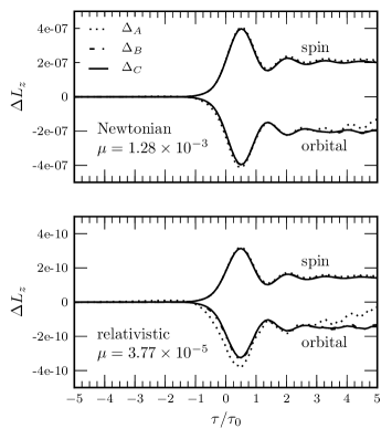
Figure 15: Total angular momentum conservation in Newtonian and relativistic simulations. The top panel shows a strictly Newtonian model while the bottom panel shows a full FNC model with our most relativistic orbit. We use an encounter strength $\eta=4$ and a mass ratio for the Newtonian case of $\mu=1.28\times 10^{-3}$ and $\mu=3.77\times 10^{-5}$ for the relativistic case. Three resolutions ($\Delta_{A},\Delta_{B},\Delta_{C}$) are shown.

VI.3 Relativistic angular momentum transfer

There are several obstacles to duplicating the above result in our full simulations (i.e., in general relativity). These include (1) defining angular momentum rigorously (i.e., in an asymptotically flat spacetime), (2) the difficulty in defining a split between spin and orbital angular momenta, and (3) the difficulties in transferring angular momentum between coordinate systems  thor1985 ; misn1973 .

The encounter between a white dwarf and IMBH can be regarded as isolated in an asymptotically flat spacetime. So total angular momentum can be defined (asymptotically) and is conserved. Furthermore, consistent with the approximations we have used, the IMBH is sufficiently massive to be regarded as stationary (Schwarzschild). The spacetime thus has Killing vectors and in particular has a rotational Killing vector $\xi_{(\phi)}^{\mu}=(\partial/\partial\phi)^{\mu}$ about the axis normal to the orbital plane. We may then form the conserved four-current $\mathscr{J}^{\mu}=T^{\mu\nu}\xi_{(\phi)\nu}$ and from it derive a conserved total angular momentum of the star (and debris)

$$J_{z}=\int\mathscr{J}^{0}\sqrt{-g}\,d^{3}X=\int d^{3}X\sqrt{-g}\,\rho\,h\,r^{2}\sin^{2}\theta\,U^{\phi}\,U^{0},$$ (92)

where $h=1+\Pi+p/\rho$ is the specific enthalpy and the integral is over a volume that encompasses all of the material.

To approximately split orbital and spin angular momenta, we view the fluid as confined to a small volume (FNC domain). The center of the frame moves on $X^{\mu}=X_{(0)}^{\mu}(\tau)$, which has constants of motion $\tilde{E}$ and $\tilde{L}$. To the extent that the gravitational mass of the star does not change and can be approximated by $M_{*}$ (order $\varepsilon^{2}$ errors), the initial orbital angular momentum will be $L_{z}^{(0)}=M_{*}r_{(0)}(t)^{2}U_{(0)}^{\phi}(t)=M_{*}\tilde{L}$, which coincides with $J_{z}$. Thus $L_{z}^{(0)}$ is the analogue of (89).

As the star passes through pericenter internal motions develop and spin is deposited in the fluid (which we compute in the FNC frame). The CM is also deflected, which affects the orbital angular momentum. If the velocity and position of the CM are transferred from the FNC frame to Schwarzschild coordinates, they can be used to form corrections $\delta X^{\mu}$ and $\delta U^{\mu}$ relative to the geodesic $X_{(0)}^{\mu}(\tau)$. We can then compute the change in the orbital angular momentum using

$$\delta L_{z}^{\text{orbital}}=M_{*}\left(r_{(0)}^{2}\delta U^{\phi}+2r_{(0)}U_{(0)}^{\phi}\delta r\right).$$ (93)

An event $(\tau,x^{i})$ in FNCs will have a Schwarzschild coordinate location $X^{\mu}$. By assumption, $X^{\mu}$ is close to $X_{(0)}^{\mu}$ and we can form an expansion

$$\delta X^{\mu}=X^{\mu}-X^{\mu}_{(0)}(\tau)=x^{i}\left(\frac{\partial X^{\mu}}{\partial x^{i}}\right)_{(0)}+\cdots.$$ (94)

Then, recognizing the tetrad frame components,

$$\delta X^{\mu}=x^{i}\lambda_{i}^{\mu}+\cdots.$$ (95)

In like fashion, the velocity $u^{a}$ at $(\tau,x^{i})$ can be transformed to components $U^{\mu}$ at the event $X^{\mu}$ by

$$U^{\mu}(X^{\nu})=\frac{\partial X^{\mu}}{\partial\tau}(\tau,x^{k})\,u^{0}+\frac{\partial X^{\mu}}{\partial x^{i}}(\tau,x^{k})\,u^{i}.$$ (96)

The transformation matrix is then expanded about FNC frame center, yielding

$$U^{\mu}(X^{\nu})=\frac{\partial X^{\mu}}{\partial\tau}(\tau,0)\,u^{0} + \frac{\partial X^{\mu}}{\partial\tau\,\partial x^{i}}(\tau,0)\,u^{0}\,x^{i}$$

$$+ \frac{\partial X^{\mu}}{\partial x^{i}}(\tau,0)\,u^{i}+\cdots.$$

We reduce this expression by recognizing first that $U_{(0)}^{\mu}=\partial X^{\mu}/\partial\tau(\tau,0)$. Secondly, in the FNC frame $u^{0}\simeq 1+\mathcal{O}(\varepsilon^{2})$ and $u^{i}=v^{i}+\mathcal{O}(\varepsilon^{3})$. Finally, $\lambda_{i}^{\ \mu}=\partial X^{\mu}/\partial x^{i}$, which allows us to write

$$\delta U^{\mu}=U^{\mu}-U^{\mu}_{(0)}=x^{i}\frac{d\lambda_{i}^{\mu}}{d\tau}+v^{i}\lambda_{i}^{\mu}+\cdots.$$ (98)

Then, we set $x^{i}=D_{i}/M_{*}$ and use (95) to calculate $\delta r$. Next we set $v^{i}=\dot{D}_{i}/M_{*}$ and use (98) to find $\delta U^{\phi}$. These are then both employed in (93) to obtain the shift in the relativistic orbital angular momentum.

The bottom panel in Figure 15 shows results from an $\eta=4$ encounter with our most relativistic orbit ($3.77\times 10^{-5}$). The top curve is the angular momentum deposited into the star. The bottom curve is from our calculation of (93) for the change in the orbital angular momentum. Three resolutions are shown and the result is well converged numerically. It is worth noting that the remarkable balance between the two in this relativistic case depends heavily on the transformations shown above. A straightforward application of the Newtonian expression (90) fails to provide an accurate measure of the compensating change.

VI.4 Energy versus angular momentum and comparison with the affine model

Having obtained both the energy and the angular momentum that are transferred in a tidal encounter, we compare the two in Fig. 16. We confirm the previously known linear relationship koch1992 ; nolt1982 , which holds over a broad range of encounter strengths. Kochanek has analyzed koch1992 the relationship within the context of ellipsoidal models and tested it through use of an affine code cart1985 ; lumi1986 . His analysis found the proportionality to be

$$\Delta E_{\rm tot}=\frac{|E_{g}|}{\sqrt{15}}\frac{\Delta L_{z}}{\sqrt{I_{*}|E_{g}|}},$$ (99)

where $E_{g}=2E_{\text{tot}}$ is the gravitational potential energy of the star. In Fig. 16 we plot this ellipsoidal model relationship (solid line) for comparison. It fails to fit full simulation results at the upper end (especially for full disruption at $\eta=1$) where linear analysis ceases to be a good approximation. Each of our simulations used mass ratio $\mu=1.28\times 10^{-3}$ and results are shown for higher resolutions $\Delta_{C}$ and $\Delta_{B}$.

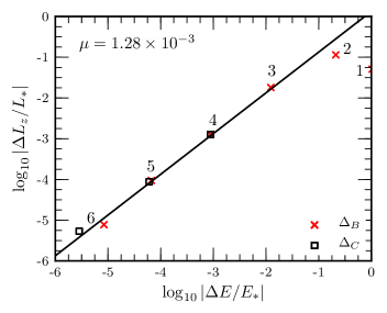
Figure 16: Tidally transferred angular momentum $\Delta L_{z}$ versus energy $\Delta E$. Angular momentum and energy normalized by $L_{*}=\sqrt{GM_{*}^{3}R_{*}}$ and $E_{*}=GM_{*}^{2}/R_{*}$, respectively. Solid line is from analysis of ellipsoidal models koch1992 . Simulations used mass ratio $\mu=1.28\times 10^{-3}$.

VII Conclusions

In this paper we investigated the tidal interactions between a white dwarf and an intermediate mass black hole. We used a Fermi normal coordinate system that provides a local moving frame roughly centered on the star. The FNC approach yields an expansion of the black hole tidal field that contains quadrupole and higher multipole moments and orbital relativistic effects. It also allows a simpler, nearly-Newtonian treatment of the star’s hydrodynamic motions and self-gravity, at least in a sufficiently confined FNC domain. We detailed which terms in the tidal field expansion are consistent with this approximation to the hydrodynamics and self-gravity. A new numerical code was constructed based around this formalism. It utilizes the well-developed PPMLR hydrodynamics method and a three-dimensional spectral method approach to solve for the self-gravitational potential.

We simulated a set of tidal models, both weak encounters and those at the threshold of disruption. At the outset, simulations were computed of our stellar equilibrium models, without a superposed tidal field, to demonstrate how “quiet” the initial models are and to establish their value as a control. We then examined the overall hydrodynamic features in tidal encounters and computed the mass loss from a white dwarf as a result of different weak encounters. For the range of black hole masses we considered in this paper, we found the $l=4$ part of the tidal field to have negligible impact. The same would not be true had we modeled white dwarf encounters with $10M_{\odot}$ to $50M_{\odot}$ black holes. The tidal field expansion also includes the gravitomagnetic term. Its effects are subtle and we intend to address those in a subsequent paper.

Besides computing the mass loss, one of the principal focuses of this paper was on transfer of energy from the orbit into the white dwarf and total energy losses from the orbit. We computed accurately the deposition of tidal energy onto the star. We then investigated where that energy resides. After comparing to the results of linear theory, we found that a combination of excitation of nonradial and radial modes and surface layer heating accounts for the energy transfer to the star. Stars that survive a tidal encounter (1) are oscillating violently in the fundamental (rotating) quadrupole mode, (2) suffer some mass loss, (3) are shock heated in their outer layers, (4) see an average reduction in their central density and an increase in their radius, and (5) develop nonlinearly an oscillation in their fundamental radial mode. We also identified a slight relativistic suppression of tidal energy transfer in the encounters with the most massive black hole we considered. All of these effects seen in our numerical models were shown to be accurately determined by considering several different finite difference resolutions. Several of these effects would make disruption more likely upon a second passage. With energy transfer to the star computed, we separately calculated the amount of energy loss from the orbit due to gravitational bremsstrahlung. We combined these losses to estimate the range of tidal capture orbits that result following weak encounters.

Lastly, we turned attention to transfer of angular momentum from the orbit into spin of the white dwarf. We computed the tidal torquing of the star and debris, and confirmed with our full numerical models the previously predicted linear relationship between transferred energy and deposited angular momentum. Then we demonstrated the result of including the octupole part of the tide in driving a deflection of the center of mass of the star (and debris), which to our knowledge is the first instance of this effect being computed in finite difference numerical models. Furthermore, we were able to take the observed CM deflection and compute directly from it the change in orbital angular momentum. The increase in spin angular momentum in the star is seen to balance nicely with decrease in orbital angular momentum. While expected physically, this result is only possible to see once enough terms are included in the tidal field. Furthermore, it is necessary to include an approximate relativistic calculation to transform effects seen in the FNC frame into changes in orbital angular momentum seen in the black hole frame.

Appendix A Numerical Method

Our numerical method for calculating tidal interactions between a massive black hole and a star consists of three parts: a module that computes the motion of the FNC frame and the tidal acceleration terms, a hydrodynamics solver, and a self-gravity module. Overall, the method combines a three-dimensional finite difference approach for the hydrodynamics and a spectral co-location technique for the self-gravity.

A.1 Motion of the FNC frame and tidal accelerations

The FNC frame center follows a timelike geodesic of the Schwarzschild background spacetime. We integrate the Darwin form of the geodesic Eqs., (13)–(18), using a Runge-Kutta routine for some set of orbital parameters (i.e., $e$ and $p$) and some initial azimuthal position $\phi$ or radial distance $R_{i}$. The position of the frame center in Schwarzschild coordinates is obtained as functions of the radial phase $\chi$. We can invert $\tau=\tau(\chi)$ and take the proper time $\tau$ instead as the curve parameter. Proper time along the geodesic becomes the time coordinate within the entire FNC frame.

Most of the effort in computing the tidal accelerations is accomplished via the derivations in Sec. II. We must integrate Eq. (24) for the frame precession angle $\Psi$ given some initially chosen orientation. The components of the Riemann tensor in the black hole frame are computed at the instantaneous position of the frame center and projected into the FNC frame using the time-dependent components of the FNC frame vectors. From this the various tidal tensors are computed and finally the tidal potential (60) and gravitomagnetic potential (61) are computed.

A.2 PPMLR hydrodynamics algorithm

We use a version of the explicit, time-dependent hydrodynamics code VH-1 blondin to solve the equations for inviscid flow of an ideal compressible gas with fixed adiabatic index $\gamma$ and with gravitational acceleration terms. The code is based on the piecewise parabolic method (PPM) of Colella and Woodward cole1984 and uses the Lagrangian-remap formulation of the method. It is an extension of Godunov’s method that offers high-order accuracy in smooth regions of the flow (third order in space and second order in time) while sharply capturing discontinuities. Our version of VH-1 was recast in C and ported to parallel machines running under MPI. The coordinate topology in the hydrodynamics code is taken to be Cartesian. We use a zero-gradient outflow boundary condition. Mass, energy, and momentum are allowed to flux out of the domain provided the local, instantaneous normal component of velocity is outward directed. Otherwise, the fluxes are set to zero.

This particular hydrodynamics technique is very standard and verification of the code follows a well-known procedure. We ran the code against a battery of standard test problems, including but not limited to (1) the Sod shock tube sod1978 , (2) twin, colliding blast waves, (3) Mach 3 wind tunnel with step, and (4) double Mach reflection of a strong shock (see Woodward and Colella wood1984 ). The results chen2012 were indistinguishable from those published previously.

The hydrodynamics code, as well as the other major elements, use domain decomposition to facilitate parallel computing. To make the algorithm simple, we have in fact chosen to divide the three-dimensional domain into slabs that are one zone deep, and farm each thin slab to an individual processor. Each processor executes the directionally split part of the algorithm along the two directions of available data, and then partially updated data is gathered to transpose the domain decomposition along another direction. A run with $N^{3}$ total spatial grid points will make use of $N$ processors. We have run a few computations on a $1024^{3}$ grid with $1024$ processors. Most of our highest resolution runs have $N=512$.

Several other tests of the hydrodynamics, when combined with the self-gravity routine, were made and these are discussed in Sec. III.3.

A.3 Pseudo-spectral self-gravity solver

Our computation of the self-gravitational field follows closely a method developed by Broderick and Rathore (brod2006, ). At our level of approximation, the gravitational field as a whole is determined by a gravitomagnetic potential $A_{k}$, a scalar tidal potential $\Phi_{\rm tidal}$, and the self-gravitational potential $\Phi$. The field $\Phi$ satisfies Poisson’s equation

$$\nabla^{2}\Phi(\vec{x})=4\pi\rho(\vec{x}),$$ (100)

where $\rho$ is the Newtonian mass density. In principle, $\Phi+\Phi_{\rm tidal}$ satisfies (100) subject to imposition of appropriate boundary conditions. However, we separately compute the tidal potential and solve the Poisson equation only for the self-gravitational field $\Phi$ subject to the condition $\Phi\rightarrow 0$ as $r\rightarrow\infty$.

We solve (100) with a discrete sine transform (DST) in three dimensions. This spectral approach serves to rapidly invert the matrix resulting from finite differencing the elliptic equation. Unfortunately, the way our boundary conditions are handled (see below) does not allow exponential convergence, one of the other primary benefits of spectral methods. Instead our solutions of (100) are second-order (algebraically) convergent, consistent with the other parts of the code.

While a Fourier transform is natural on a Cartesian mesh, matching to an asymptotically vanishing boundary condition on $\Phi$ requires some effort. Use of the DST implies that the field vanishes everywhere on the boundary of our rectangular domain. To circumvent this, the method described by Broderick and Rathore brod2006 (see also pres1996 ) crafts a one-zone-thick distribution of mass $\rho^{B}$ (image mass) in the outermost zone along each boundary face of the domain. With the right distribution of image mass the solution for $\Phi$ will approach the boundary with a fall-off that is consistent with (extrapolated) vanishing at infinity and with correct multipole content. The problem to be solved with the DST is then

$$\nabla^{2}\Phi=4\pi\left(\rho+\rho^{B}\right)=4\pi\rho_{\rm total},$$ (101)

once $\rho^{B}(\vec{x})$ is specified. We provide details in what follows, especially how our cell-centering makes for slight differences with Broderick and Rathore.

The grid consists of cell-centered data, so that the outermost points in any direction are a half zone away from the physical faces (boundaries) of the domain. For example, let $I$ be the number of zones in the $x$ direction. Let $\Delta x$ be the zone increment and $L_{x}=I\Delta x$ be the width of the domain. Then $x_{i}=(i+1/2)\Delta x$ denote the locations of the field values in the $x$ direction, with equivalent discrete locations $y_{j}$ and $z_{k}$ in the other directions. Note that while the FNC system will have its origin at the center of the domain, in order to apply the DST we make a shift temporarily so that the origin in the DST calculation is placed at a corner of the domain. The field and the source are assumed to be odd symmetric across any face. Then, given the half zone cell-centering, the forward transform is a DST of type II fftw ,

$$\hat{f}_{l}=\sum_{i=0}^{I-1}f(x_{i})\sin\left[\frac{\pi}{I}(i+1/2)(l+1)\right],$$ (102)

and the inverse transform is a DST of type III,

$$f(x_{i})=\frac{2}{I}\sum_{l=0}^{I-2}\hat{f}_{l}\sin\left[\frac{\pi}{I}(i+1/2)(l+1)\right]+\frac{(-1)^{i}}{I}\hat{f}_{I-1}.$$ (103)

We can easily generalize from one dimension to three, but do so in a way that enables parallel computing. Let $I,J,K$ be the number of zones in the $x$, $y$, and $z$ directions. Let $i,j,k$ distinguish the spatial locations like before but now with $y_{j}=(j+1/2)\Delta y$ and $z_{k}=(k+1/2)\Delta z$. The corresponding discrete points in the transform space are indexed by $l,m,n$. The discrete three-dimensional sine transform of, say, $\rho$ can be accomplished in three steps, each of which is a DST-II and can be computed in parallel given a slab decomposition of the domain:

$$u_{ljk} = \sum_{i=0}^{I-1}\rho_{ijk}\sin\left[\frac{\pi}{I}(i+1/2)(l+1)\right],$$

$$v_{lmk} = \sum_{j=0}^{J-1}u_{ljk}\sin\left[\frac{\pi}{J}(j+1/2)(m+1)\right],$$

$$\hat{\rho}_{lmn} = \sum_{k=0}^{K-1}v_{lmk}\sin\left[\frac{\pi}{K}(k+1/2)(n+1)\right].$$ (104)

Then, if from $\hat{\rho}_{lmn}$ we have determined $\hat{\Phi}_{lmn}$, we can reverse the process in parallel with a DST-III transform to find $\Phi_{ijk}$,

$$w_{lmk} = \frac{2}{K}\sum_{n=0}^{K-2}\hat{\Phi}_{lmn}\sin\left[\frac{\pi}{K}(k+1/2)(n+1)\right]$$

$$+\frac{(-1)^{k}}{K}\hat{\Phi}_{lm,K-1}$$

$$y_{ljk} = \frac{2}{J}\sum_{m=0}^{J-2}w_{lmk}\sin\left[\frac{\pi}{J}(j+1/2)(m+1)\right]$$

$$+\frac{(-1)^{j}}{J}w_{l,J-1,k}$$

$$\Phi_{ijk} = \frac{2}{I}\sum_{l=0}^{I-2}y_{ljk}\sin\left[\frac{\pi}{I}(i+1/2)(l+1)\right]$$ (105)

$$+\frac{(-1)^{i}}{I}y_{I-1,j,k}.$$

We derive the algebraic connection between $\hat{\rho}_{lmn}$ and $\hat{\Phi}_{lmn}$ using a centered, second-order finite difference expression

$$\left(\nabla^{2}\Phi\right)_{ijk} = (\Phi_{i+1,jk}-2\Phi_{ijk}+\Phi_{i-1,jk})/(\Delta x)^{2}$$ (106)

$$+(\Phi_{i,j+1,k}-2\Phi_{ijk}+\Phi_{i,j-1,k})/(\Delta y)^{2}$$

$$+(\Phi_{ij,k+1}-2\Phi_{ijk}+\Phi_{ij,k-1})/(\Delta z)^{2}$$

$$= 4\pi\rho_{ijk}.$$

Upon substituting the Fourier transform we obtain

$$\hat{\Phi}_{lmn}=-4\pi\frac{\hat{\rho}_{lmn}}{\kappa_{lmn}^{2}},$$ (107)

where

$$\kappa_{lmn}^{2} = \frac{2}{(\Delta x)^{2}}\left[1-\cos\left(\frac{\pi(l+1)}{I}\right)\right]$$

$$+\frac{2}{(\Delta y)^{2}}\left[1-\cos\left(\frac{\pi(m+1)}{J}\right)\right]$$

$$+\frac{2}{(\Delta z)^{2}}\left[1-\cos\left(\frac{\pi(n+1)}{K}\right)\right],$$

which is unchanged from Broderick and Rathore. Note that determining $\kappa_{lmn}$ using (106) immediately makes the method algebraically convergent, but as we will see this is consistent with our handling of the boundary conditions.

We next consider how to trick the DST into providing a solution with an appropriate, asymptotically-falling $\mathcal{O}(1/r)$ field at the boundary of the domain. This starts with deciding what the field at the boundary should be. We rely on most of the mass being confined to the inner region of the domain and use a multipole expansion up to some order $l_{\rm max}$

$$\Phi^{B}(\vec{x})=-\sum^{l_{max}}_{l=0}\sum^{l}_{m=-l}\frac{4\pi}{2l+1}r^{-(l+1)}Q_{lm}Y_{lm}(\theta,\phi),$$ (108)

to give an approximation for the asymptotic field once we have obtained a set of source moments

$$Q_{lm}=\int d^{3}x^{\prime}{r^{\prime}}^{l}Y^{*}_{lm}(\theta^{\prime},\phi^{\prime})\rho(\vec{x}^{\prime}).$$

We find $l_{\rm max}=5$ is typically sufficient.

Given the assumptions implicit in use of the DST (odd symmetry across each face of the domain), with little mass density near the boundary the field will approach the boundary linearly and vanish. In our discrete representation the field at the ultimate physical zone (say $\Phi_{0,jk}$) will be odd-symmetric with respect to the field in the neighboring ghost zone (in this case $\Phi_{-1,jk}$). The trick is to introduce a boundary mass distribution $\rho^{B}$ in the outermost physical zones that generates just the right kink in the discrete field so that $\Phi\simeq\Phi^{B}$ in the ultimate physical zones while still being consistent with the odd symmetry at each domain face.

We can illustrate this in one dimension. Let $i=0$ be the first physical cell at $x=+\Delta x/2$. The DST requires that the field vanish at $x=0$, which is not at a field sample but corresponds to fractional location $i=-1/2$. Instead, if we carry a neighboring ghost zone at $x=-\Delta x/2$ ($i=-1$), the field there satisfies $\Phi_{-1}=-\Phi_{0}$. The average between these two, the implied value on the domain boundary, is of course zero. Now imagine instead that the first few field samples ($\Phi_{2}$, $\Phi_{1}$, and $\Phi_{0}$) trend smoothly toward some (nonzero) $\Phi^{B}=\Phi^{B}_{-1/2}$ assumed to exist at $x=0$. If we smoothly extrapolate to the first ghost zone we would have an implied value there of

$$\Phi^{*}_{-1}=2\Phi^{B}_{-1/2}-\Phi_{0}.$$ (109)

If we evaluated (106) in the ultimate ($i=0$) location we would write

$$\Phi^{*}_{-1,jk} - 2\Phi_{0,jk}+\Phi_{1,jk}$$

$$= \Delta x^{2}\left(4\pi\rho-\partial_{y}^{2}\Phi-\partial_{z}^{2}\Phi\right)_{0jk}.$$

In a solution to the elliptic system the last two equations could be combined to “close the mesh” and encode the desired boundary condition. In using the DST though, (109) violates the required antisymmetry. To get around this, substitute (109) into (A.3) and insert the DST-required condition $\Phi_{-1}=-\Phi_{0}$ to obtain

$$\Phi_{-1,jk} - 2\Phi_{0,jk}+\Phi_{1,jk}$$

$$= (\Delta x)^{2}\left(4\pi\rho-\partial_{y}^{2}\Phi-\partial_{z}^{2}\Phi\right)_{0,jk}-2\Phi^{B}_{-1/2,jk}.$$

We can interpret this last piece on the right-hand side as a source $\rho^{B}_{0,jk}$, where

$$\rho_{0,jk}^{B}=-\frac{2\Phi_{-1/2,jk}}{4\pi(\Delta x)^{2}},$$ (112)

that adds to the real mass density $\rho$. This image mass density is one zone thick. The implied loss of differentiability in $\Phi$ is the primary reason why the spectral method will not converge exponentially, and is in this case algebraic and second order.

The discussion above was confined to one face of the domain. We generalize by placing image mass density in the outermost zones on all six faces of the computational domain,

$$4\pi\rho^{B}_{ijk}= - \frac{2}{(\Delta x)^{2}}\left(\delta_{i,0}\Phi^{B}_{-1/2,jk}+\delta_{i,I-1}\Phi^{B}_{I-1/2,jk}\right)$$

$$- \frac{2}{(\Delta y)^{2}}\left(\delta_{j,0}\Phi^{B}_{i,-1/2,k}+\delta_{j,J-1}\Phi^{B}_{i,J-1/2,k}\right)$$

$$- \frac{2}{(\Delta z)^{2}}\left(\delta_{k,0}\Phi^{B}_{ij,-1/2}+\delta_{k,K-1}\Phi^{B}_{ij,K-1/2}\right).$$

Given our cell centering, this image distribution differs from Broderick and Rathore by a factor of 2. Once $\Phi$ has been determined within the domain, extrapolated values can be placed in the surrounding ghost zones [e.g., (109)] as needed.

To test the Poisson solver, a set of compact density distributions are constructed that have associated known analytic solutions for $\Phi$. The mass is confined within a sphere of unit radius near the center of the domain. The density is tapered to zero sufficiently smoothly so as to not affect the order of convergence of the method boyd2001 . Each test distribution has a different angular multipole and since the equation is linear we use a superposition

$$\rho=\sum_{l=0}c_{l}r^{l}\left(1-r^{2}\right)^{3}P_{l}(\cos\gamma),\qquad{\rm for\ }r<1,$$ (114)

where $\rho=0$ for $r>1$. Different orientations ($\gamma$) can be tested, as well as different relative multipole strengths $c_{l}$. We tested configurations where $l=0$ dominated and ones where it did not contribute significantly. In our highest resolution test with domain length $L=4$ in three dimensions with $512^{3}$ zones, the local error is less than 0.1% over most of the domain.

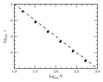
Figure 17: Convergence of $L_{2}$ error between numerical $\Phi^{\rm num}$ and analytic $\Phi^{\rm analytic}$ solutions of a self-gravity test problem. The $L_{2}$ error is plotted against number of zones, $N$, in one direction. The total number of zones in a model is $N^{3}$. The method exhibits second-order convergence.

The solution should converge at second-order rate as the number of grid points or basis functions increases. The behavior is illustrated in Fig. 17. Consider a domain with equal length sides $L$. Take $I=J=K=N$. The total number of grid locations is $N^{3}$. The $L_{2}$ error is

$$\varepsilon=\left[\frac{1}{N^{3}}\sum_{ijk}\left(\Phi^{\rm num}_{ijk}-\Phi^{\rm analytic}_{ijk}\right)^{2}\right]^{1/2}.$$ (115)

Figure 17 shows strict second-order convergence in the $L_{2}$ error over a range of five doublings of $N$.

Appendix B Octupole tidal tensor in the FNC frame

The nonzero components of the octupole tidal tensor in the FNC frame for parabolic $\tilde{E}=1$ orbits are given by

$$C_{111} = \frac{3M}{4r^{4}}\Big{[}3\left(1+\frac{7\tilde{L}^{2}}{3r^{2}}\right)\cos\Psi+5\left(1+\frac{\tilde{L}^{2}}{r^{2}}\right)\cos 3\Psi-6\frac{\tilde{L}}{r}U^{r}\left(1+\frac{5\tilde{L}^{2}}{3r^{2}}\right)\sin\Psi$$

$$- 10\frac{\tilde{L}}{r}U^{r}\left(1+\frac{\tilde{L}^{2}}{r^{2}}\right)\cos 2\Psi\,\sin\Psi\Big{]}V_{2}^{-1}$$

$$C_{131} = C_{311}=C_{113}=\frac{M}{4r^{4}}\Big{[}\frac{\tilde{L}}{r}U^{r}\left(1+\frac{5\tilde{L}^{2}}{r^{2}}\right)\cos\Psi+15\frac{\tilde{L}}{r}U^{r}\left(1+\frac{\tilde{L}^{2}}{r^{2}}\right)\cos 3\Psi$$

$$+ 18\left(1+\frac{11\tilde{L}^{2}}{9r^{2}}\right)\sin\Psi+30\left(1+\frac{\tilde{L}^{2}}{r^{2}}\right)\cos 2\Psi\,\sin\Psi\Big{]}V_{2}^{-1}$$

$$C_{122} = C_{212}=C_{221}=\frac{M}{r^{4}}\Big{[}-3\left(1+\frac{7\tilde{L}^{2}}{3r^{2}}\right)\cos\Psi+\frac{\tilde{L}}{r}U^{r}\left(1+\frac{5\tilde{L}^{2}}{r^{2}}\right)\sin\Psi\Big{]}V_{2}^{-1}$$

$$C_{133} = C_{313}=C_{331}=\frac{M}{4r^{4}}\Big{[}3\left(1+\frac{7\tilde{L}^{2}}{3r^{2}}\right)\cos\Psi-15\left(1+\frac{\tilde{L}^{2}}{r^{2}}\right)\cos 3\Psi$$

$$+ 14\frac{\tilde{L}}{r}U^{r}\left(1+\frac{5\tilde{L}^{2}}{7r^{2}}\right)\sin\Psi+30\frac{\tilde{L}}{r}U^{r}\left(1+\frac{\tilde{L}^{2}}{r^{2}}\right)\cos 2\Psi\,\sin\Psi\Big{]}V_{2}^{-1}$$

$$C_{322} = C_{232}=C_{223}=-\frac{M}{r^{4}}\Big{[}\frac{\tilde{L}}{r}U^{r}\left(1+\frac{5\tilde{L}^{2}}{r^{2}}\right)\cos\Psi+3\left(1+\frac{7\tilde{L}^{2}}{3r^{2}}\right)\sin\Psi\Big{]}V_{2}^{-1}$$

$$C_{333} = \frac{3M}{4r^{4}}\Big{[}\frac{\tilde{L}}{r}U^{r}\left(1+\frac{5\tilde{L}^{2}}{r^{2}}\right)\cos\Psi-5\frac{\tilde{L}}{r}U^{r}\left(1+\frac{\tilde{L}^{2}}{r^{2}}\right)\cos 3\Psi$$ (116)

$$- 12\left(1+\frac{2\tilde{L}^{2}}{3r^{2}}\right)\sin\Psi+20\left(1+\frac{\tilde{L}^{2}}{r^{2}}\right)\sin^{3}\Psi\Big{]}V_{2}^{-1}.$$

References

- (1) M. J. Rees, Nature 333, 523 (Jun. 1988)
- (2) S. Komossa, J. Halpern, N. Schartel, G. Hasinger, M. Santos-Lleo, and P. Predehl, ApJL 603, L17 (Mar. 2004), arXiv:astro-ph/0402468
- (3) J. Magorrian and S. Tremaine, MNRAS 309, 447 (Oct. 1999), arXiv:astro-ph/9902032
- (4) J. Wang and D. Merritt, Astrophys. J. 600, 149 (Jan. 2004), arXiv:astro-ph/0305493
- (5) B. Carter and J. P. Luminet, Nature 296, 211 (Mar. 1982)
- (6) E. S. Phinney, in The Center of the Galaxy, IAU Symposium, Vol. 136, edited by M. Morris (1989) p. 543
- (7) C. R. Evans and C. S. Kochanek, ApJL 346, L13 (Nov. 1989)
- (8) L. E. Strubbe and E. Quataert, MNRAS 400, 2070 (Dec. 2009), arXiv:0905.3735 [astro-ph.CO]
- (9) A. M. Beloborodov, A. F. Illarionov, P. B. Ivanov, and A. G. Polnarev, MNRAS 259, 209 (Nov. 1992)
- (10) M. Kesden, Phys. Rev. D 85, 024037 (Jan. 2012), arXiv:1109.6329 [astro-ph.CO]
- (11) D. Grupe, H.-C. Thomas, and K. M. Leighly, A&A 350, L31 (Oct. 1999), arXiv:astro-ph/9909101
- (12) S. Komossa and N. Bade, A&A 343, 775 (Mar. 1999), arXiv:astro-ph/9901141
- (13) J. Greiner, R. Schwarz, S. Zharikov, and M. Orio, A&A 362, L25 (Oct. 2000), arXiv:astro-ph/0009430
- (14) J. P. Halpern, S. Gezari, and S. Komossa, Astrophys. J. 604, 572 (Apr. 2004), arXiv:astro-ph/0402497
- (15) P. Esquej, R. D. Saxton, M. J. Freyberg, A. M. Read, B. Altieri, M. Sanchez-Portal, and G. Hasinger, A&A 462, L49 (Feb. 2007), arXiv:astro-ph/0612340
- (16) N. Cappelluti, M. Ajello, P. Rebusco, S. Komossa, A. Bongiorno, C. Clemens, M. Salvato, P. Esquej, T. Aldcroft, J. Greiner, and H. Quintana, A&A 495, L9 (Feb. 2009), arXiv:0901.3357 [astro-ph.CO]
- (17) S. Komossa, H. Zhou, A. Rau, M. Dopita, A. Gal-Yam, J. Greiner, J. Zuther, M. Salvato, D. Xu, H. Lu, R. Saxton, and M. Ajello, Astrophys. J. 701, 105 (Aug. 2009), arXiv:0902.3248 [astro-ph.GA]
- (18) W. P. Maksym, M. P. Ulmer, and M. Eracleous, Astrophys. J. 722, 1035 (Oct. 2010), arXiv:1008.4140 [astro-ph.HE]
- (19) J. R. Cummings, S. D. Barthelmy, A. P. Beardmore, D. N. Burrows, S. Campana, V. D’Elia, P. A. Evans, N. Gehrels, J. M. Gelbord, C. Guidorzi, S. T. Holland, E. A. Hoversten, J. A. Kennea, H. A. Krimm, O. M. Littlejohns, R. Margutti, F. E. Marshall, A. Melandri, C. Pagani, K. L. Page, D. M. Palmer, P. Romano, M. H. Siegel, E. Sonbas, R. L. C. Starling, G. Stratta, G. Tagliaferri, and E. Troja, GRB Coordinates Network 11823, 1 (Mar. 2011)
- (20) S. B. Cenko, H. A. Krimm, A. Horesh, A. Rau, D. A. Frail, J. A. Kennea, A. J. Levan, S. T. Holland, N. R. Butler, R. M. Quimby, J. S. Bloom, A. V. Filippenko, A. Gal-Yam, J. Greiner, S. R. Kulkarni, E. O. Ofek, F. Olivares E., P. Schady, J. M. Silverman, N. Tanvir, and D. Xu, ArXiv e-prints(Jul. 2011), arXiv:1107.5307 [astro-ph.HE]
- (21) A. Renzini, L. Greggio, S. di Serego Alighieri, M. Cappellari, D. Burstein, and F. Bertola, Nature 378, 39 (Nov. 1995)
- (22) S. Gezari, S. Basa, D. C. Martin, G. Bazin, K. Forster, B. Milliard, J. P. Halpern, P. G. Friedman, P. Morrissey, S. G. Neff, D. Schiminovich, M. Seibert, T. Small, and T. K. Wyder, Astrophys. J. 676, 944 (Apr. 2008), arXiv:0712.4149
- (23) S. Gezari, T. Heckman, S. B. Cenko, M. Eracleous, K. Forster, T. S. Gonçalves, D. C. Martin, P. Morrissey, S. G. Neff, M. Seibert, D. Schiminovich, and T. K. Wyder, Astrophys. J. 698, 1367 (Jun. 2009), arXiv:0904.1596 [astro-ph.CO]
- (24) S. van Velzen, G. R. Farrar, S. Gezari, N. Morrell, D. Zaritsky, L. Östman, M. Smith, J. Gelfand, and A. J. Drake, Astrophys. J. 741, 73 (Nov. 2011), arXiv:1009.1627 [astro-ph.CO]
- (25) S. Gezari, R. Chornock, A. Rest, M. E. Huber, K. Forster, E. Berger, P. J. Challis, J. D. Neill, D. C. Martin, T. Heckman, A. Lawrence, C. Norman, G. Narayan, R. J. Foley, G. H. Marion, D. Scolnic, L. Chomiuk, A. Soderberg, K. Smith, R. P. Kirshner, A. G. Riess, S. J. Smartt, C. W. Stubbs, J. L. Tonry, W. M. Wood-Vasey, W. S. Burgett, K. C. Chambers, T. Grav, J. N. Heasley, N. Kaiser, R.-P. Kudritzki, E. A. Magnier, J. S. Morgan, and P. A. Price, Nature 485, 217 (May 2012), arXiv:1205.0252 [astro-ph.CO]
- (26) B. A. Zauderer, E. Berger, A. M. Soderberg, A. Loeb, R. Narayan, D. A. Frail, G. R. Petitpas, A. Brunthaler, R. Chornock, J. M. Carpenter, G. G. Pooley, K. Mooley, S. R. Kulkarni, R. Margutti, D. B. Fox, E. Nakar, N. A. Patel, N. H. Volgenau, T. L. Culverhouse, M. F. Bietenholz, M. P. Rupen, W. Max-Moerbeck, A. C. S. Readhead, J. Richards, M. Shepherd, S. Storm, and C. L. H. Hull, Nature 476, 425 (Aug. 2011), arXiv:1106.3568 [astro-ph.HE]
- (27) A. J. Levan, N. R. Tanvir, S. B. Cenko, D. A. Perley, K. Wiersema, J. S. Bloom, A. S. Fruchter, A. d. U. Postigo, P. T. O’Brien, N. Butler, A. J. van der Horst, G. Leloudas, A. N. Morgan, K. Misra, G. C. Bower, J. Farihi, R. L. Tunnicliffe, M. Modjaz, J. M. Silverman, J. Hjorth, C. Thöne, A. Cucchiara, J. M. C. Cerón, A. J. Castro-Tirado, J. A. Arnold, M. Bremer, J. P. Brodie, T. Carroll, M. C. Cooper, P. A. Curran, R. M. Cutri, J. Ehle, D. Forbes, J. Fynbo, J. Gorosabel, J. Graham, D. I. Hoffman, S. Guziy, P. Jakobsson, A. Kamble, T. Kerr, M. M. Kasliwal, C. Kouveliotou, D. Kocevski, N. M. Law, P. E. Nugent, E. O. Ofek, D. Poznanski, R. M. Quimby, E. Rol, A. J. Romanowsky, R. Sánchez-Ramírez, S. Schulze, N. Singh, L. van Spaandonk, R. L. C. Starling, R. G. Strom, J. C. Tello, O. Vaduvescu, P. J. Wheatley, R. A. M. J. Wijers, J. M. Winters, and D. Xu, Science 333, 199 (Jul. 2011), arXiv:1104.3356 [astro-ph.HE]
- (28) J. S. Bloom, D. Giannios, B. D. Metzger, S. B. Cenko, D. A. Perley, N. R. Butler, N. R. Tanvir, A. J. Levan, P. T. O’Brien, L. E. Strubbe, F. De Colle, E. Ramirez-Ruiz, W. H. Lee, S. Nayakshin, E. Quataert, A. R. King, A. Cucchiara, J. Guillochon, G. C. Bower, A. S. Fruchter, A. N. Morgan, and A. J. van der Horst, Science 333, 203 (Jul. 2011), arXiv:1104.3257 [astro-ph.HE]
- (29) D. N. Burrows, J. A. Kennea, G. Ghisellini, V. Mangano, B. Zhang, K. L. Page, M. Eracleous, P. Romano, T. Sakamoto, A. D. Falcone, J. P. Osborne, S. Campana, A. P. Beardmore, A. A. Breeveld, M. M. Chester, R. Corbet, S. Covino, J. R. Cummings, P. D’Avanzo, V. D’Elia, P. Esposito, P. A. Evans, D. Fugazza, J. M. Gelbord, K. Hiroi, S. T. Holland, K. Y. Huang, M. Im, G. Israel, Y. Jeon, Y.-B. Jeon, H. D. Jun, N. Kawai, J. H. Kim, H. A. Krimm, F. E. Marshall, P. Mészáros, H. Negoro, N. Omodei, W.-K. Park, J. S. Perkins, M. Sugizaki, H.-I. Sung, G. Tagliaferri, E. Troja, Y. Ueda, Y. Urata, R. Usui, L. A. Antonelli, S. D. Barthelmy, G. Cusumano, P. Giommi, A. Melandri, M. Perri, J. L. Racusin, B. Sbarufatti, M. H. Siegel, and N. Gehrels, Nature 476, 421 (Aug. 2011), arXiv:1104.4787 [astro-ph.HE]
- (30) G. Lodato, A. R. King, and J. E. Pringle, MNRAS 392, 332 (Jan. 2009), arXiv:0810.1288
- (31) K. Hayasaki, N. Stone, and A. Loeb, ArXiv e-prints(Oct. 2012), arXiv:1210.1333 [astro-ph.HE]
- (32) S. Kobayashi, P. Laguna, E. S. Phinney, and P. Mészáros, Astrophys. J. 615, 855 (Nov. 2004), arXiv:astro-ph/0404173
- (33) W. H. Press and S. A. Teukolsky, Astrophys. J. 213, 183 (1977)
- (34) A. Khokhlov and F. Melia, ApJL 457, L61+ (Feb. 1996)
- (35) D. Kasen and E. Ramirez-Ruiz, Astrophys. J. 714, 155 (May 2010), arXiv:0911.5358 [astro-ph.HE]
- (36) Y. Rathore, R. D. Blandford, and A. E. Broderick, MNRAS 357, 834 (Mar. 2005), arXiv:astro-ph/0406102
- (37) S. Rosswog, E. Ramirez-Ruiz, and W. R. Hix, Astrophys. J. 695, 404 (Apr. 2009), arXiv:0808.2143
- (38) R. A. Nolthenius and J. I. Katz, Astrophys. J. 263, 377 (Dec. 1982)
- (39) G. V. Bicknell and R. A. Gingold, Astrophys. J. 273, 749 (Oct. 1983)
- (40) P. Laguna, W. A. Miller, W. H. Zurek, and M. B. Davies, ApJL 410, L83 (Jun. 1993)
- (41) S. Ayal, M. Livio, and T. Piran, Astrophys. J. 545, 772 (Dec. 2000), arXiv:astro-ph/0002499
- (42) A. Khokhlov, I. D. Novikov, and C. J. Pethick, Astrophys. J. 418, 163 (Nov. 1993)
- (43) A. Khokhlov, I. D. Novikov, and C. J. Pethick, Astrophys. J. 418, 181 (Nov. 1993)
- (44) V. P. Frolov, A. M. Khokhlov, I. D. Novikov, and C. J. Pethick, Astrophys. J. 432, 680 (Sep. 1994)
- (45) J. A. Marck, A. Lioure, and S. Bonazzola, A&A 306, 666 (Feb. 1996), arXiv:astro-ph/9505027
- (46) P. Diener, V. P. Frolov, A. M. Khokhlov, I. D. Novikov, and C. J. Pethick, Astrophys. J. 479, 164 (Apr. 1997)
- (47) J. Guillochon, E. Ramirez-Ruiz, S. Rosswog, and D. Kasen, Astrophys. J. 705, 844 (Nov. 2009), arXiv:0811.1370
- (48) B. Carter and J.-P. Luminet, A&A 121, 97 (May 1983)
- (49) J.-P. Luminet and B. Carter, Astrophys. J. Suppl. Ser. 61, 219 (Jun. 1986)
- (50) C. S. Kochanek, Astrophys. J. 385, 604 (Feb. 1992)
- (51) P. B. Ivanov and I. D. Novikov, Astrophys. J. 549, 467 (Mar. 2001), arXiv:astro-ph/0005107
- (52) P. B. Ivanov, M. A. Chernyakova, and I. D. Novikov, MNRAS 338, 147 (Jan. 2003), arXiv:astro-ph/0205065
- (53) T. Bogdanović, M. Eracleous, S. Mahadevan, S. Sigurdsson, and P. Laguna, Astrophys. J. 610, 707 (Aug. 2004), arXiv:astro-ph/0404256
- (54) R. Haas, R. V. Shcherbakov, T. Bode, and P. Laguna, Astrophys. J. 749, 117 (Apr. 2012), arXiv:1201.4389 [astro-ph.HE]
- (55) R. V. Shcherbakov, A. Pe’er, C. S. Reynolds, R. Haas, T. Bode, and P. Laguna, ArXiv e-prints(Dec. 2012), arXiv:1212.4837 [astro-ph.HE]
- (56) J. H. Krolik and T. Piran, Astrophys. J. 743, 134 (Dec. 2011), arXiv:1106.0923 [astro-ph.HE]
- (57) J. H. Krolik and T. Piran, Astrophys. J. 749, 92 (Apr. 2012), arXiv:1111.2802 [astro-ph.HE]
- (58) M. Ishii, M. Shibata, and Y. Mino, Phys. Rev. D 71, 044017 (Feb. 2005), arXiv:gr-qc/0501084
- (59) C. Misner, K. Thorne, and J. Wheeler, Gravitation (W.H. Freeman, San Francisco, 1973)
- (60) F. K. Manasse and C. W. Misner, Journal of Mathematical Physics 4, 735 (Jun. 1963)
- (61) B. Mashhoon, Astrophys. J. 197, 705 (May 1975)
- (62) J. Marck, Royal Society of London Proceedings Series A 385, 431 (Feb. 1983)
- (63) E. Poisson, A relativist’s toolkit : the mathematics of black-hole mechanics (Cambridge University Press, Cambridge, 2004)
- (64) K. S. Thorne and J. B. Hartle, Phys. Rev. D 31, 1815 (Apr. 1985)
- (65) C. Darwin, Royal Society of London Proceedings Series A 249, 180 (Jan. 1959)
- (66) C. Cutler, D. Kennefick, and E. Poisson, Phys. Rev. D 50, 3816 (Sep. 1994)
- (67) L. G. Fishbone, Astrophys. J. 185, 43 (Oct. 1973)
- (68) S. Detweiler and E. Poisson, Phys. Rev. D 69, 084019 (Apr. 2004)
- (69) J. P. Cox, Theory of stellar pulsation (Princeton University Press, Princeton, NJ, 1980)
- (70) D. Bale, R. J. LeVeque, S. Mitran, and J. A. Rossmanith, SIAM J. Sci. Comput. 24, 955 (2003), http://epubs.siam.org/sam-bin/dbq/article/39738
- (71) B. Carter and J. P. Luminet, MNRAS 212, 23 (Jan. 1985)
- (72) H. M. Lee and J. P. Ostriker, Astrophys. J. 310, 176 (Nov. 1986)
- (73) S. F. Portegies Zwart and A. T. Meinen, A&A 280, 174 (Dec. 1993)
- (74) P. C. Peters, Physical Review 136, 1224 (Nov. 1964)
- (75) J. Blondin, J. Hawley, G. Lindahl, and E. Lufkin, “ Virginia Hydrodynamics 1 (VH-1),” (2012), http://wonka.physics.ncsu.edu/pub/VH-1/
- (76) P. Colella and P. R. Woodward, Journal of Computational Physics 54, 174 (Sep. 1984)
- (77) G. A. Sod, Journal of Computational Physics 27, 1 (Apr. 1978)
- (78) P. Woodward and P. Colella, Journal of Computational Physics 54, 115 (Apr. 1984)
- (79) R. M. Cheng, Tidal Disruption of a Star By a Massive Black Hole Computed In Fermi Normal Coordinates, Ph.D. thesis, University of North Carolina at Chapel Hill (2012)
- (80) A. E. Broderick and Y. Rathore, MNRAS 372, 923 (Oct. 2006), arXiv:astro-ph/0411652
- (81) W. Press, S. Teukolsky, W. Vettering, and B. Flannery, Numerical Recipes in C: The Art of Parallel Scientific Computing (Cambridge University Press, Cambridge, 1996)
- (82) M. Frigo and S. G. Johnson, “Fastest Fourier Transform in the West (FFTW),” (2012), http://www.fftw.org/
- (83) J. P. Boyd, Chebyshev and Fourier Spectral Methods (Dover Publications, Inc., Mineola, New York, 2001)