On quasi–linear PDAEs with convection:
applications, indices, numerical solution

Abstract

For a class of partial differential algebraic equations (PDAEs) of quasi–linear type which include nonlinear terms of convection type a possibility to determine a time and spatial index is considered. As a typical example we investigate an application from plasma physics. Especially we discuss the numerical solution of initial boundary value problems by means of a corresponding finite difference splitting procedure which is a modification of a well known fractional step method coupled with a matrix factorization. The convergence of the numerical solution towards the exact solution of the corresponding initial boundary value problem is investigated. Some results of a numerical solution of the plasma PDAE are given.

,

1 Introduction

In this paper quasi–linear PDAEs for $u=u(t,x),~{}x\in\Omega:=(0,1),$ of the form

$$Au_{t}+Bu_{xx}+C[u]u_{x}+Du= f(t,x),\quad t\in(0,t_{e}),~{}~{}~{}~{}x\in\Omega,$$ (1)

for some $t_{e}>0$ are considered. $~{}u$ and $f$ are mappings $~{}u,f:~{}[0,t_{e}]\times\bar{\Omega}\rightarrow{\Rset}^{n},~{}~{}n\geq 1,$ where $f$ (supposed to be sufficiently smooth) is given. $A,~{}B,~{}C[u]$ and $D$ are real $(n,n)-$matrices where $A,~{}B$ and $D$ are assumed to be constant. All matrices may be singular, but $A,~{}B\neq 0$. $C[u]$ may depend on $u$. We suppose that it is linear in $u$. Typically, when $C[u]$ is linear in $u$, vector $C[u]u_{x}$ describes physical convection.
For system (1) we study classical initial boundary value problems (IBVPs). Initial values (IVs) may be decomposed

$$u(0,x) =\Phi_{a}(x)+\Phi_{c}(x),\quad x\in\bar{\Omega}$$ (2)

$$\Phi_{a,k}(x)= \begin{cases}u_{k}(0,x)\quad u_{k}(0,x)\quad\hbox{can be prescribed arbitrarily}\\ 0\hskip 22.76228pt\qquad\hbox{otherwise,}\end{cases}$$

$$\Phi_{c,k}(x)= \begin{cases}u_{k}(0,x)\quad u_{k}(0,x)\quad\hbox{cannot be prescribed arbitrarily}\\ 0\hskip 22.76228pt\qquad\hbox{otherwise,}\end{cases}$$

with ($k=1,...,n$). The boundary values (BVs) are of similar form,

$$u(t,x)= \Psi_{a}(t,x)+\Psi_{c}(t,x),\quad t\in[0,t_{e}],\quad x\in\partial\Omega=\{0,1\}.$$ (3)

This means the data which can be prescribed arbitrarily are in $\Phi_{a},~{}\Psi_{a}$. The consistent data (see e.g. [2] or [12]) are collected in $\Phi_{c},~{}\Psi_{c}$. Furthermore, we assume that the compatibility relations

$$\Phi_{a}(x)+\Phi_{c}(x)=\Psi_{a}(0,x)+\Psi_{c}(0,x),\quad x\in\partial\Omega,$$ (4)

are satisfied. Because almost every PDAE has its own IV and BV distribution we avoid here to give a more detailed general description of these data. In section 5 we solve this problem for the plasma PDAE considered in the next section.
This paper is organized as follows. In section 2 a nonlinear PDAE from physics is presented. In section 3 known general index concepts applicable also to nonlinear PDAEs are considered. The numerical solution of IBVPs by a finite difference splitting method is studied in section 4. Especially, convergence results are given. A numerical example from plasma physics is presented in section 5.

2 An application

In this section we cite a mathematical model from plasma physics [7, Chapter 5] whose underlying system of equations is of type (1). It describes the space–time–movement of a system consisting of ions (with mass $m_{i}$, density $n_{i}$ and positive electrical charge $q$) and electrons (with density $n_{e}$ and electrical charge $-q$) in the space domain $\Omega$. The charge $q(n_{e}-n_{i})$ produces an electrical potential $\phi$ such that the ions move under the corresponding electrical force $-q\phi_{x}$. The system of electrons is considered to be a gas with (constant) temperature $T_{e}$ and pressure $p=k_{B}T_{e}n_{e}$ where $k_{B}$ is Boltzmann’s constant. The relation between $n_{e}$ and $\phi$ is given by the equilibrium of electrical and mechanical forces,

$$qn_{e}\phi_{x}-k_{B}T_{e}n_{e,x}=0,~{}$$

and the equations of conservation of mass and momentum for the ions are

$$n_{i,t}+(n_{i}v_{i})_{x}-D_{i}n_{i,xx}=0\quad\mathrm{and}\quad m_{i}\left(\frac{\partial}{\partial t}+v_{i}\frac{\partial}{\partial x}\right)v_{i}+q\phi_{x}=0,$$

respectively. $D_{i}$ is a (constant) diffusion coefficient, and $v_{i}$ is the velocity of the ions. The equation for $\phi$ is Poisson’s equation

$$\phi_{xx}-4\pi(n_{e}-n_{i})=0.$$

It is convenient to transform this system of equations by a linear transformation into a new system of the form (1) with $n=4,~{}~{}f=0$ and new dependent variables $u_{i}$ and with matrices

$$A=\left(\begin{smallmatrix}1&0&0&0\\ 0&1&0&0\\ 0&0&0&0\\ 0&0&0&0\end{smallmatrix}\right),~{}B= \left(\begin{smallmatrix}-b_{0}&0&0&0\\ 0&0&0&0\\ 0&0&0&0\\ 0&0&0&1\end{smallmatrix}\right),~{}C[u]=\left(\begin{smallmatrix}u_{2}&u_{1}&0&0\\ 0&u_{2}&0&d_{1}\\ 0&0&-1&u_{3}\\ 0&0&0&0\end{smallmatrix}\right),~{}D=\left(\begin{smallmatrix}0&0&0&0\\ 0&0&0&0\\ 0&0&0&0\\ 1&0&-1&0\end{smallmatrix}\right).$$ (5)

The new variables $u_{i}$ are (up to a constant) given by $u_{1}\sim n_{i},~{}~{}u_{2}\sim v_{i},~{}~{}u_{3}\sim n_{e},~{}~{}u_{4}\sim\phi.$ $b_{0}\geq 0$ and $d_{1}>0$ are constants.
Note that the matrices $A,~{}B$ are diagonal and singular, and $C[u]$ is linear in the components of $u$ (for short we say that $C[u]$ is linear in $u$).
Further examples of a system of type (1) are a poroelastic model of a living bone [5, 6, 10] and the incompressible Navier–Stokes equations if eq. (1) is generalized in obvious manner to two and three space dimensions.

3 Indices

First we introduce two definitions of classical linear spaces. Let $l,~{}m$ be nonnegative integers, and let $C_{sc}^{l,m}$ be the space of scalar real functions $w(t,x),~{}~{}t\in[0,t_{e}],~{}~{}x\in\overline{\Omega}$, whose derivatives up to the $(l+m)^{th}$ order (time derivatives up to the $l^{th}$ order and space derivatives up to the $m^{th}$ order) are continuous. With $C_{sc}^{l,m}$ the set

$$C^{l,m}_{n}:=\left\{w=(w_{1},...,w_{n})^{T};~{}~{}~{}w_{i}\in C_{sc}^{l,m},~{}~{}i=1,...,n\right\}$$

is defined. By $C_{n,0}^{l,m}$ we denote a set of vector valued functions with vanishing BVs,

$$C^{l,m}_{n,0}:=\Big{\{}w\in C_{n}^{l,m};\quad w(t,0)=w(t,1)=0\Big{\}}.$$

While the index of linear PDAEs has been considered by several authors, e.g. [2, 3, 4, 8, 12, 13], the index for nonlinear systems is investigated little, see however [11] where a discretization based index definition has been given, and [14]. We mention that we do not transform system (1) to a first order system because we prefer in numerical calculations the original second order form.
In this paper, a well known index concept for PDAEs is used to construct certain operators whose invertibility (if so) yields indices. The basic notion of a time index $\nu_{t}$ and a spatial index $\nu_{x}$ can be found, e.g., in [3, 12, 14].
Throughout this paper the time index $\nu_{t}$ of (1) is of special interest. We assume that a solution u of the IBVP (1) – (4) exists and that $u$ is sufficiently differentiable. Furthermore, we suppose that $u(t,x)=0~{}$ for $~{}x\in\partial\Omega.$ When $\Psi_{a}$ and $\Psi_{c}$ (see eq. (3)) are known, zero BVs can be obtained by a suitable transformation of $u$.

3.1 Time index

Definition 1

If the matrix $A$ is regular, the time index $\nu_{t}$ of the PDAE (1) is defined to be zero. If $A$ is singular, then $\nu_{t}$ is the smallest number of times the PDAE must be differentiated with respect to $t$ in order to determine $u_{t}$ as a continuous function of $t,~{}x,~{}u$ and certain space derivatives of $u-$components.

Since in most practical applications of PDAEs the time index is $\nu_{t}=1$ or $\nu_{t}=2$, we give here the formalism for these two indices for PDAEs of type (1) only. First, an auxiliary result is stated. To simplify the notation we use in the following the summation convention (summation about twofold indices from $1$ to $n$).

Lemma 2

Let $u$ be sufficiently smooth, and suppose that $C[u]$ is linear in $u$. Then

1. $\partial_{t}C[u]u_{x}=C^{(1)}[u_{x}]u_{t}+C[u]u_{tx}$ where $C^{(1)}_{ik}[u_{x}]:=C_{ij,k}u_{j,x}$,

2. $\partial_{t}C^{(1)}[u_{x}]u_{t}=C^{(1)}[u_{tx}]u_{t}+C^{(1)}[u_{x}]u_{tt}.$

[Proof.] Let $C_{ij,k}:=\frac{\partial C_{ij}}{\partial u_{k}},~{}i,j,k\in\{1,\dots,n\}.$ Componentwise differentiation with respect to time yields

$$\partial_{t}C_{ij}u_{j,x}=C_{ij,k}u_{k,t}u_{j,x}+C_{ij}u_{j,tx}=(C_{ij,k}u_{j,x})u_{k,t}+C_{ij}u_{j,tx}.$$

Statement (I) follows from the definition of $C^{(1)}_{ik}$. Using this definition again and the linearity of $C$ in $u$ we get

$$\partial_{t}C^{(1)}_{ik}[u_{x}]u_{k,t}= C_{ij,k}u_{j,tx}u_{k,t}+C_{ij,k}u_{j,x}u_{k,tt}= C^{(1)}_{ik}[u_{tx}]u_{k,t}+C_{ik}^{(1)}[u_{x}]u_{k,tt}$$

which is (II) in component form.∎ For example, $C[u]$ given in (5) produces $C^{(1)}[u_{x}]=\left(\begin{smallmatrix}u_{2,x}&u_{1,x}&0&0\\ 0&u_{2,x}&0&0\\ 0&0&u_{4,x}&0\\ 0&0&0&0\end{smallmatrix}\right).~{}$
With this Lemma and with definitions

$$L:= B\partial^{2}_{x}+D,\qquad M[u,u_{x}]:=L+C^{(1)}[u_{x}]+C[u]\partial_{x}$$

we find formally from eq. (1) under the assumptions of Lemma 2 after one time differentiation (this case is relevant for $\nu_{t}=1$) the derivative array

$$\displaystyle\left(\begin{matrix}A&0\\ M[u,u_{x}]&A\end{matrix}\right)\displaystyle\left(\begin{matrix}u_{t}\\ u_{tt}\end{matrix}\right)+\displaystyle\left(\begin{matrix}Lu+C[u]u_{x}\\ 0\end{matrix}\right)= \displaystyle\left(\begin{matrix}f\\ f_{t}\end{matrix}\right).$$ (6)

Two time differentiations of (1) produce the derivative array (for $\nu_{t}=2$)

$$\displaystyle\left(\begin{matrix}A&0&0\\ M[u,u_{x}]&A&0\\ 2C^{(1)}[u_{tx}]&M[u,u_{x}]&A\end{matrix}\right)\displaystyle\left(\begin{matrix}u_{t}\\ u_{tt}\\ u_{ttt}\end{matrix}\right)+\displaystyle\left(\begin{matrix}Lu+C[u]u_{x}\\ 0\\ 0\end{matrix}\right)=\displaystyle\left(\begin{matrix}f\\ f_{t}\\ f_{tt}\end{matrix}\right).$$ (7)

When $A$ is singular, the coefficient matrices (denoted by $\mathcal{A}$) of the systems (6), (7) are singular in the sense that ${\mathcal{A}}v=0$ where $v\neq 0$ is an appropriate vector function (e.g. in the case of eq. (6), $v=(u_{t}^{T},u_{tt}^{T})^{T},~{}u\in C^{2,2}_{n}$). However, the coefficient matrices might uniquely determine $u_{t}$. The analogous problem for linear time varying DAEs (differential algebraic equations) is discussed in [1, p. 29], and for linear PDAEs of first order it is investigated in [14].
For the nonlinear PDAE (1), the derivative array (6) or (7) is used to write

$$Pu_{t}= F$$ (8)

where $P$ is according to eq. (6) or (7) an operator valued matrix, and the vector $F$ does not depend on $u_{t}$. First, we must find $P$ and an appropriate domain of definition $D(P)$. Second, the invertibility of $P$ must be studied.
We mention, that the matrix $P$ in equation (8) is the analogue to the nonsingular diagonal matrix $D(x_{j})$ defined in [14], Definition 3.5. However, here we need not require a diagonal form of $P$.

3.2 Spatial index

If $B$ is singular, we suppose that the PDAE is written in quasilinear form (with respect to second space derivatives), i.e. we transform $B$ according to $\overline{B}=S_{0}BS_{1}^{-1}=\left(\begin{smallmatrix}I_{m}&0\\ 0&0\end{smallmatrix}\right)$ where $S_{0},~{}S_{1}$ are constant regular $(n,n)-$matrices.

Definition 3

The spatial index $\nu_{x}$ of a system with a regular matrix $B$ is defined to be zero. When $B$ is singular, $\nu_{x}$ is the smallest number of times the PDAE

$$\overline{A}\overline{u}_{t}+\overline{B}\overline{u}_{xx}+\overline{C}[S_{1}^{-1}\overline{u}]\overline{u}_{x}+\overline{D}\overline{u}=\overline{f}(t,x)$$

($\overline{u}=S_{1}u,~{}\overline{A}=S_{0}AS_{1}^{-1}$, and so on) must be differentiated with respect to $x$ in order to obtain

$$\overline{U}:=(\underbrace{\overline{u}_{1,xx},\overline{u}_{2,xx},...,\overline{u}_{m,xx}}_{m~{}~{}elements},\underbrace{\overline{u}_{{n_{1}+1},x},...,\overline{u}_{n,x}}_{n-m~{}~{}elements})^{T}$$

as a continuous function of $~{}~{}t,~{}x,~{}\overline{u},~{}\overline{u}_{t}$ and $\bar{u}_{1,x},\dots,\bar{u}_{m,x}$.

It is straightforward to derive for $\overline{U}$ a derivative array (by differentiations of the PDAE with respect to $x$) analogous to eq. (6) or (7). As a result, after a minimal number of $x-$differentiations one can find a representation of $\overline{U}$ of the form $\overline{Q}~{}\overline{U}=\overline{G}$ where $\overline{Q}$ is an operator valued matrix. The vector $\overline{G}$ is independent of the components of $\overline{U}$. This definition of the spatial index is according to the one given in [12]. It does not transform the PDAE (1) to a system of first order as is often done, e.g. in [14]. Such a transformation, in general, changes the indices. For example, one can show that the time-index here is $0$ if and only if the corresponding index in [14] is $1$, a time-index $1$ or $2$ here implies an index $2$ there.

3.3 Time index of the plasma PDAE

Here, we study the time index $\nu_{t}$ of the PDAE (1) under the assumption of zero BVs, $u(t,0)=u(t,1)=0,~{}$ and $f\in C_{4}^{p,q}$ with suitable $p,~{}q.~{}$ To be specific we further assume that this IBVP has a solution $u\in C_{4,0}^{1,2}$ which possibly exists only local in time. To determine the time index of system (1) we generate for $\nu_{t}$ – if possible – system (8) with the condition that $P$ defined on $D(P)$ is invertible. In order to determine $\nu_{t}$ we differentiate the third and fourth equation of the PDAE with respect to $t$ with the result

$$-u_{3,tx}+u_{3,t}u_{4,x}+u_{3}u_{4,tx}=0\;\;\hbox{and}\;\;u_{4,txx}+u_{1,t}-u_{3,t}=0.$$

A new system can be formed by means of these two equations and the first two equations of the original system. This is a closed system of four equations for the components of $u_{t}$ in terms of $u$ and derivatives which are not time derivatives of $u-$components. Obviously, the new system can be written

$$Pu_{t}=F(u):= \left(\begin{smallmatrix}-u_{2}u_{1,x}-u_{1}u_{2,x}+b_{0}u_{1,xx}\\ -u_{2}u_{2,x}-d_{1}u_{4,x}\\ 0\\ 0\end{smallmatrix}\right),~{}P:= \left(\begin{smallmatrix}1&0&0&0\\ 0&1&0&0\\ 0&0&[-\partial_{x}+u_{4,x}]&u_{3}\partial_{x}\\ 1&0&-1&\partial^{2}_{x}\end{smallmatrix}\right).$$ (9)

Now what is essential for the determination of the index of the PDAE is that $u$ in $P$ can be seen as a fixed element with the result that $P:~{}D(P)\rightarrow R(P)$, $D(P)\subset C_{4,0}^{1,2}$, is a linear operator ($R(P)$ denotes the range of $P$). We can try to solve the first equation in (9) for $u_{t}$ by standard linear theory. In particular, if $P^{-1}$ exists we get $\nu_{t}$ as the least number of time differentiations which are necessary to get the equation for $u_{t}$ (in the example considered here, one differentiation with respect to $t$ is needed).

Remark 4

The right hand side of the first equation in (9) does not play any role when $\nu_{t}$ is to be determined. This implies that $\nu_{t}$ is independent of $f$ in equation (1). This is a reasonable result because the right hand side function should not influence the indices of a PDAE.

We ask whether the linear operator $P$ with $D(P)\subset C_{4,0}^{1,3}$ has for fixed $u=u(t,x)$ an inverse. The answer comes from kernel $N(P)$ whose elements $z$ fulfill

$$Pz=\left(\begin{smallmatrix}z_{1}\\ z_{2}\\ -z_{3,x}+u_{4,x}z_{3}+u_{3}z_{4,x}\\ z_{1}-z_{3}+z_{4,xx}\end{smallmatrix}\right)=0.$$

This reduces to $z_{1}=z_{2}=0$ and a linear homogeneous coupled system of two ordinary differential equations for $z_{3}$ and $z_{4},$ $-z_{3,x}+u_{4,x}z_{3}+u_{3}z_{4,x}=0$ and $-z_{3}+z_{4,xx}=0,$ with homogeneous BVs, $z_{3}(0)=0$ and $z_{4}(0)=z_{4}(1)=0.~{}$ $~{}z_{4}$ is also a solution of the equation $-z_{4,xxx}+u_{4,x}z_{4,xx}+u_{3}z_{4,x}=0$ which can be reduced to $-y_{xx}+u_{4,x}y_{x}+u_{3}y=0$ where $y=y(t,x):=z_{4,x}(t,x).$ By $\varphi_{1}$ and $\varphi_{2}$ we denote two fundamental solutions of the equation for $y$, i.e. $y=K_{1}\varphi_{1}+K_{2}\varphi_{2}$ is the general solution ($K_{i},~{}i=1,2,$ are independent of $x$). Then the following Lemma holds:

Lemma 5

Let $u$ be such that $\left|\displaystyle\begin{matrix}\varphi_{1,x}(0)&\varphi_{2,x}(0)\\ \int\limits_{0}^{1}\varphi_{1}(\xi)d\xi&\int\limits_{0}^{1}\varphi_{2}(\xi)d\xi\end{matrix}\right|~{}\neq~{}0.$
Then $z_{3}~{}=z_{4}~{}=~{}0.$

Since the proof is simple, it is omitted here (for details see [10]).
Under the assumptions of this Lemma we see that $N(P)=\{0\}$. Therefore, system (9) can be solved for $u_{t}$, and the time index is $\nu_{t}=1$.
We mention that based on Definition 3 the spatial index of the plasma PDAE can be determined similarly. The result is $\nu_{x}=0.~{}~{}$

4 Numerical solution by a finite difference method

In this section we consider the numerical solution of IBVPs (1) – (4) by means of a fractional step difference method which is combined with a matrix factorization. The fractional step method and numerous variants of it are well known, see e.g. [9]. By this method, the order of the system of equations which must be solved can be reduced considerably. The effort can be reduced further by a proper partition of the original system matrix (denoted by $L$ below) into two splitting matrices ($L=L_{1}+L_{2}$).
To describe the general procedure, we first rewrite the nonlinear part $C[u]u_{x}$ of the PDAE (1) as $C[u,\partial_{x}]u$ which is more convenient sometimes. $C[u,\partial_{x}]$ is an operator valued matrix. For example, with $C[u]$ given in (5) it is

$$C[u]u_{x}=\displaystyle\left(\begin{matrix}u_{2}&u_{1}&0&0\\ 0&u_{2}&0&d_{1}\\ 0&0&-1&u_{3}\\ 0&0&0&0\end{matrix}\right)\textstyle\left(\begin{matrix}u_{1,x}\\ u_{2,x}\\ u_{3,x}\\ u_{4,x}\end{matrix}\right)= \displaystyle\left(\begin{matrix}\partial_{x}u_{2}&0&0&0\\ 0&u_{2}\partial_{x}&0&d_{1}\partial_{x}\\ 0&0&-\partial_{x}&u_{3}\partial_{x}\\ 0&0&0&0\end{matrix}\right)\displaystyle\left(\begin{matrix}u_{1}\\ u_{2}\\ u_{3}\\ u_{4}\end{matrix}\right)=:C[u,\partial_{x}]u.$$

We suppose that $A$ is singular and is given as $A=\left(\begin{smallmatrix}I_{n_{1}}&0\\ 0&0\end{smallmatrix}\right)$  where $I_{n_{1}}$ is the unit matrix of order $n_{1}<n$ $(n_{1}\geq 1).$ Let $n_{2}=n-n_{1}.$ Corresponding to this partition of $A$ we introduce the notation $u=(u_{1},~{}u_{2})^{T}~{}$ and $M=\left(\begin{smallmatrix}M_{11}&M_{12}\\ M_{21}&M_{22}\end{smallmatrix}\right)$ where the $(n,n)-$matrix $M$ may be one of the matrices $B,~{}C,~{}D$. The component representation of $u_{k}$ is $u_{k}=(u_{k1}^{T},...,u_{kn_{k}}^{T})^{T},~{}k=1,2.$ According to this partition, PDAE (1) is written

$$\displaystyle\left(\begin{matrix}I_{n_{1}}&0\\ 0&0\end{matrix}\right)u_{t}+\displaystyle\left(\begin{matrix}B_{11}&B_{12}\\ B_{21}&B_{22}\end{matrix}\right)u_{xx}+\displaystyle\left(\begin{matrix}C_{11}[u,\partial_{x}]&C_{12}[u,\partial_{x}]\\ C_{21}[u,\partial_{x}]&C_{22}[u,\partial_{x}]\end{matrix}\right)u+\displaystyle\left(\begin{matrix}D_{11}&D_{12}\\ D_{21}&D_{22}\end{matrix}\right)u=f.$$ (10)

Furthermore, let the operator valued matrices $L_{k}[u],~{}k=1,2,~{}$ be defined by ($C_{kj}=C_{kj}[u,\partial_{x}]$)

$$L_{1}[u]:= \displaystyle\left(\begin{matrix}0&0\\ (B_{21}\partial^{2}_{x}+C_{21}+D_{21})&(B_{22}\partial^{2}_{x}+C_{22}+D_{22})\end{matrix}\right),$$ (11)

$$L_{2}[u]:= \displaystyle\left(\begin{matrix}(B_{11}\partial_{x}^{2}+C_{11}+D_{11})&(B_{21}\partial^{2}_{x}+C_{21}+D_{21})\\ 0&0\end{matrix}\right)$$ (12)

such that $L[u]~{}:=~{}B\partial^{2}_{x}+C[u,\partial_{x}]+D~{}=~{}L_{1}[u]+L_{2}[u].$

Remark 6

Sometimes, other operators $L_{1}$, $L_{2}$ with $L=L_{1}+L_{2}$ may be more convenient because the solution of the equations may be easier. In every case, the partition should be such that the identity $AL_{2}=L_{2}$ does hold. This is needed in a factorization as explained below in eq. (16).

In order to obtain an approximate numerical solution of IBVP (1) – (4) we consider it with zero BVs (3) by means of a difference method. The first time derivative is approximated with an equidistant time step size $\tau$ by

$$u_{t}(t_{m+1},x_{k})\approx\frac{1}{\tau}(u^{m+1}(x_{k})-u^{m}(x_{k})),\quad t_{m+1}=(m+1)\tau,\quad m=0,1,...$$

The corresponding IBVP is space discretized on an equidistant grid

$$\Omega_{h}:=\{x_{k}=kh,~{}k=0,1,...,M;~{}~{}h=1/M,~{}M>1\}$$

by using difference formulas ($k=1,...,M-1$)

$$u_{xx}(t,x_{k})\approx \frac{\delta^{2}}{h^{2}}u_{k}(t):=\frac{1}{h^{2}}\big{(}u_{k-1}(t)-2u_{k}(t)+u_{k+1}(t)\big{)},$$

$$u_{x}(t,x_{k})\approx \frac{\delta_{0}}{2h}u_{k}(t)\quad\hbox{or}\quad\frac{\delta_{+}}{h}u_{k}(t)\quad\hbox{or}\quad\frac{\delta_{-}}{h}u_{k}(t)$$ (13)

where $\delta_{0},~{}\delta_{+}$ and $\delta_{-}$ are the usual central, forward and backward difference operators, respectively. Now suppose $t\in(0,t_{e})$, $t_{e}>0$. We approximate eq. (1) by the difference equation ($m=0,1,...,~{}~{}~{}k=1,...,M-1$)

$$A\frac{u_{k}^{m+1}-u_{k}^{m}}{\tau}+L_{h}[u_{k}^{m}]u_{k}^{m+1}= f_{k}^{m+1}.$$ (14)

$L_{h}[u_{k}^{m}]$ denotes a discretization of $L[u(t_{m},x_{k})].$ We rewrite this equation as

$$\left(A+\tau L_{h}[u^{m}_{k}]\right)\frac{u_{k}^{m+1}-u_{k}^{m}}{\tau}=f_{k}^{m+1}-L_{h}[u^{m}_{k}]u^{m}_{k}$$ (15)

and factorize approximately for $\tau\rightarrow 0$

$$A+\tau L_{h}[u_{k}^{m}]\approx(A+\tau L_{h1}[u_{k}^{m}])(I+\tau L_{h2}[u_{k}^{m}])$$ (16)

$$= A+\tau(L_{h1}[u_{k}^{m}]+AL_{h2}[u^{m}_{k}])+O(\tau^{2})=A+\tau L_{h}[u^{m}_{k}]+O(\tau^{2}),$$

where $L_{h1}$ and $L_{h2}$ are corresponding discretizations of (11) and (12), respectively (we used $AL_{h2}=L_{h2}$ and $L_{h1}+L_{h2}=L_{h}$). $u_{k}^{m}$ is considered to be an approximation for $u(t_{m},x_{k})$. Therefore, we study for $m=0,1,...$, $k=1,...,M-1$ fractional splitting

$$\left(A+\tau L_{h1}[u^{m}_{k}]\right)u_{k}^{m+1/2}= f_{k}^{m+1}-L_{h}[u^{m}_{k}]u_{k}^{m},$$ (17)

$$\left(I+\tau L_{h2}[u^{m}_{k}]\right)\frac{u_{k}^{m+1}-u_{k}^{m}}{\tau}= u_{k}^{m+1/2}.$$ (18)

$u_{k}^{0}$ is (for every $k$) given as IV.

Remark 7

This discussion shows that the fractional step method requires the solution of two linear systems of coupled equations, but each of them is, in numerous applications, of a considerably reduced order.

The approximate factorization (16) implies the following Lemma.

Lemma 8

Suppose

1. $v=v(t,x)\in{\Rset}^{n},~{}t\in(0,t_{e}),$ is for some $t_{e}>0$ the exact solution (sufficiently smooth) of the IBVP (10), (2) – (4),

2. the system of algebraic equations (17), (18) has a unique solution.

Then the method (17), (18) and the system (15) are equivalent for $\tau\rightarrow 0$, i.e. eqs. (17), (18) approximate the original system to the same $\tau-$order as eq. (15).

4.1 Convergence of the fractional step method

We consider the convergence of the numerical solution $u_{k}^{m}$ calculated by the scheme (14) towards the exact solution $v(t_{m},x_{k})$ of the corresponding IBVP for $\tau\rightarrow 0$ and $h\rightarrow 0$ under the condition $~{}(m+1)\tau=t~{}~{}(t~{}~{}\mbox{fixed}).~{}$ The basic assumption is that $C[v]=C^{0}+C^{1}[v]$ is linear in $v$ where the matrix $C^{0}=const.$ is chosen in such a manner that the matrices $G_{0k}$, $k=1,...,M-1,$ defined below in (39) are regular. For example, a proper choice may be $C^{0}=C[\bar{v}],$ $C^{1}[v]=C[v]-C[\bar{v}]$ where vector $\bar{v}$ does not depend on $t$ and $x,$ e.g. $\bar{v}$ is a suitable mean value of $v$.
First, we need the full truncation error $\alpha_{k}^{m+1}$ defined for $~{}m=0,1,...,$
$k=1,...,M-1$ by

$$\alpha_{k}^{m+1}:= A\frac{v_{k}^{m+1}-v_{k}^{m}}{\tau}+L_{h}[v_{k}^{m}]v_{k}^{m+1}-f_{k}^{m+1}$$ (19)

where $L_{h}[v^{m}_{k}]:=B\frac{\delta^{2}}{h^{2}}+C[v_{k}^{m}]\frac{\delta}{qh}+D,$ and $q=1$ (for one–sided differences) or $q=2$ (for central differences). $\delta$ stands for $\delta_{0}$ or $\delta_{+}$ or $\delta_{-}.$ Under the assumption that $v$ is sufficiently smooth we Taylor expand $v^{m}_{k},~{}v^{m}_{k\pm 1}$ in $t_{m+1}$ and $x_{k}$ to get in lowest order with respect to $\tau$ and $h$

$$\alpha_{k}^{m+1}= A(v_{k,t}^{m+1}-\frac{1}{2}v_{k,tt}^{m+1}\tau+O(\tau^{2}))+B(v_{k,xx}^{m+1}+\frac{1}{12}v_{k,xxxx}^{m+1}h^{2}+O(h^{4}))$$

$$+C[v_{k}^{m+1}-v_{k,t}^{m+1}\tau+O(\tau^{2})](v_{k,x}^{m+1}+\bar{O}^{m+1}(h^{q}))+Dv_{k}^{m+1}-f_{k}^{m+1}.$$

Since $C[v_{k}^{m+1}-v_{k,t}^{m+1}\tau]=C^{0}+C^{1}[v_{k}^{m+1}]-\tau C^{1}[v_{k,t}^{m+1}]~{}$ and
$~{}Av_{k,t}^{m+1}+Bv_{k,xx}^{m+1}+\big{(}C^{0}+C^{1}[v_{k}^{m+1}]\big{)}v_{k,x}^{m+1}+Dv_{k}^{m+1}=f_{k}^{m+1},~{}$ the truncation error can be written

$$\alpha_{k}^{m+1}= A\bar{O}^{m+1}(\tau)+B\bar{O}^{m+1}(h^{2})+C[v_{k}^{m+1}]\bar{O}^{m+1}(h^{q})$$ (20)

$$+C^{1}[v_{k,t}^{m+1}]\bar{O}^{m+1}(\tau h^{q})+C^{1}[v_{k,t}^{m+1}]\bar{O}^{m+1}(\tau).$$

Here, e.g., $\bar{O}^{m+1}(\tau)=\tau w,~{}w\in\Rset^{n},~{}w$ independent of $\tau$. Second, scheme (14) is written by means of the Kronecker product in matrix form,

$$\Big{(}I_{M-1}\otimes\frac{A}{\tau}+ Q_{h}[U^{m}]\Big{)}U^{m+1}=\Big{(}I_{M-1}\otimes\frac{A}{\tau}\Big{)}U^{m}+F^{m+1},$$ (21)

$$Q_{h}[U^{m}]:= \frac{1}{h^{2}}P\otimes B+\frac{1}{qh}\tilde{P}_{q}\otimes C[U^{m}]+I_{M-1}\otimes D$$

where $U^{m}:=(u_{1}^{mT},...,u_{M-1}^{mT})^{T},\quad F^{m}:=(f_{1}^{mT},...,f_{M-1}^{mT})^{T},~{}$ and

$$P:= \left(\begin{smallmatrix}-2&1&&\\ 1&-2&1&\\ &&\ddots&\\ &&1&-2&\end{smallmatrix}\right)\in\Rset^{(M-1)\times(M-1)}.$$ (22)

$q$ and $~{}\tilde{P}_{q}~{}$ depend on the discretization of the first space derivative. For example, using central difference formula in (13), it is $q=2$ and

$$\tilde{P}:=\left(\begin{smallmatrix}0&1&&\\ -1&0&1&\\ &&\ddots&\\ &&-1&0&\end{smallmatrix}\right)\in\Rset^{(M-1)\times(M-1)}~{}$$

(another differencing is chosen in (35)). The $(n(M-1),n(M-1))-$matrix $\tilde{P}_{q}\otimes C[U^{m}]$ is a block matrix whose block at position $(j,k)$ is $\tilde{P}_{q,jk}C[u_{j}^{m}],$ $u_{j}^{m}\in\Rset^{n}.$ Eqs. (19) and (20) imply that $~{}V^{m+1}$ satisfies equation

$$\Big{(}I_{M-1}\otimes\frac{A}{\tau}+ Q_{h}[V^{m}]\Big{)}V^{m+1}=\Big{(}I_{M-1}\otimes\frac{A}{\tau}\Big{)}V^{m}+F^{m+1}+{\mathcal{A}}^{m+1},$$ (23)

$${\mathcal{A}}^{m+1}:= E_{1}O^{m+1}(\tau)+E_{2}O^{m+1}(h^{2})+E_{3}^{m+1}O^{m+1}(h^{q})$$ (24)

$$+E_{4}^{m+1}\left[O^{m+1}(\tau h^{q})+O^{m+1}(\tau)\right]$$

where $E_{1}:=I_{M-1}\otimes A,~{}~{}E_{2}:=I_{M-1}\otimes B,~{}~{}E_{3}^{j+1}:=I_{M-1}\otimes C[V^{j+1}],$
$E_{4}^{j+1}:=I_{M-1}\otimes C^{1}[V_{t}^{j+1}]$ and, e.g., $O^{m+1}(\tau)$ means $O^{m+1}(\tau)\in{\Rset}^{n(M-1)}.$ The foregoing relations can be used to estimate a norm of the global error $\eta^{m}:=V^{m}-U^{m}$. In the following we choose the discrete $L_{2}-$norm defined for a vector $v=(v_{1},...,v_{n(M-1)})^{T}$ by $||v||:=\left[h\sum_{k=1}^{n(M-1)}{v_{k}^{2}}\right]^{1/2}.~{}$
Subtracting eq. (21) from eq. (23), we obtain

$$\left(I_{M-1}\otimes\frac{A}{\tau}\right)\eta^{m+1}+Q_{h}[V^{m}]V^{m+1}-Q_{h}[U^{m}]U^{m+1}= \left(I_{M-1}\otimes\frac{A}{\tau}\right)\eta^{m}+{\mathcal{A}}^{m+1}.$$

By the identity

$$Q_{h}[V^{m}]V^{m+1}-Q_{h}[U^{m}]U^{m+1}=\big{(}Q_{h}[V^{m}]-Q_{h}[U^{m}]\big{)}V^{m+1}+Q_{h}[U^{m}]\big{(}V^{m+1}-U^{m+1}\big{)},$$

the foregoing equation can be written

$$G^{m}\eta^{m+1}= \left(I_{M-1}\otimes\frac{A}{\tau}\right)\eta^{m}-\left(Q_{h}[V^{m}]-Q_{h}[U^{m}]\right)V^{m+1}+{\mathcal{A}}^{m+1},$$ (25)

$$G^{m}:= I_{M-1}\otimes\frac{A}{\tau}+\frac{1}{h^{2}}P\otimes B+\frac{1}{qh}\tilde{P}_{q}\otimes C[U^{m}]+I_{M-1}\otimes D.$$ (26)

Now we use the fact that

$$Q_{h}[V^{m}]-Q_{h}[U^{m}]=\frac{1}{qh}\tilde{P}_{q}\otimes\left(C[V^{m}]-C[U^{m}]\right)=\frac{1}{qh}\tilde{P}_{q}\otimes C^{1}[\eta^{m}]$$

(because the linearity of $C[u]$ implies $C[V^{m}]-C[U^{m}]=C^{1}[\eta^{m}]$). Furthermore, one can construct a $(n(M-1),n(M-1))-$matrix $\tilde{C}[V^{m+1}]$ such that

$$\left(\tilde{P}_{q}\otimes C^{1}[\eta^{m}]\right)V^{m+1}=\tilde{C}[V^{m+1}]\eta^{m}.$$

Therefore, eq. (25) takes the form ($G^{-m}=(G^{m})^{-1}$)

$$\eta^{m+1}= G^{-m}\left(I_{M-1}\otimes\frac{A}{\tau}-\frac{1}{qh}\tilde{C}[V^{m+1}]\right)\eta^{m}+G^{-m}{\mathcal{A}}^{m+1}$$

or for short

$$~{}\eta^{m+1}=H^{m}\eta^{m}+R^{m+1},\quad H^{m}:=G^{-m}\left(I_{M-1}\otimes\frac{A}{\tau}-\frac{1}{qh}\tilde{C}[V^{m+1}]\right),$$

$\quad R^{m+1}:=G^{-m}{\mathcal{A}}^{m+1}.~{}$ It follows for $m=0,1,...$

$$\eta^{m+1}=H^{m}H^{m-1}...H^{0}\eta^{0}+H^{m}H^{m-1}...H^{1}R^{1}+...+H^{m}R^{m}+R^{m+1},$$

$$||\eta^{m+1}||\leq ||H^{m}H^{m-1}...H^{0}||~{}||\eta^{0}||+||H^{m}H^{m-1}...H^{1}||~{}||R^{1}||$$ (27)

$$+||H^{m}H^{m-1}...H^{2}||~{}||R^{2}||+...+||H^{m}||~{}||R^{m}||+||R^{m+1}||.$$

Now we require for $0<m\tau=t\in(0,t_{e}]$ that

$$\sup_{m\in{\mathbb{N}}}\left\{||H^{m}H^{m-1}...H^{j}||,~{}~{}j=1,...,m\right\}~{}<~{}\infty,$$ (28)

possibly under a restriction of one of the forms

$$\kappa_{0}\leq\frac{\tau}{h}\leq\kappa_{1}, \qquad\kappa_{2}\leq\frac{\tau}{h^{2}}\leq\kappa_{3}.$$ (29)

Assumption (28) is discussed shortly in Remark 12. With this condition, the right hand side in (27) can be estimated further to give

$$||\eta^{m+1}|| \leq K_{0}||\eta^{0}||+\bar{K}_{1}\sum_{j=0}^{m}{||R^{j+1}||}\leq K_{0}||\eta^{0}||+(m+1)\bar{K}_{1}\max_{j\in[0,m]}||R^{j+1}||$$

$$\leq K_{0}||\eta^{0}||+K_{1}\frac{t}{\tau}\max_{j\in[0,m]}||R^{j+1}||.$$ (30)

$K_{0},~{}K_{1},~{}\bar{K}_{1}$ are constants. Using $||R^{j+1}||=||G^{-j}{\mathcal{A}}^{j+1}||,$ relation (24) yields

$$||R^{j+1}||\leq ||G^{-j}E_{1}||O(\tau)+||G^{-j}E_{2}||O(h^{2})+||G^{-j}E_{3}^{j+1}||O(h^{q})$$ (31)

$$+||G^{-j}E_{4}^{j+1}||\left[O(\tau h^{q})+O(\tau)\right]$$

or also

$$||R^{j+1}||\leq ||G^{-j}||\Big{(}||E_{1}||O(\tau)+||E_{2}||O(h^{2})+||E_{3}^{j+1}||O(h^{q})$$ (32)

$$+||E_{4}^{j+1}||\left[O(\tau h^{q})+O(\tau)\right]\Big{)}.$$

Note that ineq. (31) is sharper than ineq. (32). Since the matrices $E_{l}$ are block diagonal, their norms can be estimated easily. For example, $E_{3}^{j+1}$ is of the form
$E_{3}^{j+1}=diag\{C[v_{1}^{j+1}],...,C[v_{M-1}^{j+1}]\}$, and

$$||E_{3}^{j+1}||=\left[\max_{k}\left[\lambda_{max}(C^{T}[v_{k}^{j+1}]C[v_{k}^{j+1}])\right]\right]^{1/2}$$

where $\lambda_{max}(E)$ is the largest eigenvalue of $E$. Especially, if $v$ is sufficiently smooth for some time $t\leq t_{e}$, then all norms $||E_{l}||$ are bounded. Therefore, (32) can be written also

$$||R^{j+1}||\leq K_{3}||G^{-j}||\left(O(\tau)+O(h^{2})+O(h^{q})+O(\tau h^{q})\right)$$

with some constant $K_{3}$.
An estimate of $||G^{-j}||$ can be based on the eigenvectors $\phi_{k}$ of the symmetric matrix $\frac{1}{h^{2}}P$. By definition, $\frac{1}{h^{2}}P\phi_{k}=\lambda_{k}\phi_{k},~{}~{}k=1,...,M-1$. The eigenvalues are given by $\lambda_{k}=-\frac{4}{h^{2}}\sin^{2}\left(\frac{k\pi}{2M}\right)$. They fulfill for $h\to 0$ the asymptotic relation $\lambda_{k}=-(k\pi)^{2}+O(h^{2})$ (because $h=1/M$). The set $\{\phi_{k},~{}~{}k=1,...,M-1\}$ is assumed to be orthonormal. Let $\Phi:=\sqrt{h}(\phi_{1},...,\phi_{M-1})$ be the matrix of the eigenvectors and $\Lambda:=diag(\lambda_{1},...,\lambda_{M-1}).$ Since $\Phi^{-1}=\Phi^{T}=\Phi,~{}$ it follows that (for short $\Psi_{n}:=\Phi\otimes I_{n}$)

$$\frac{1}{h^{2}}P\otimes B= \Psi_{n}(\Lambda\otimes B)\Psi_{n},$$ (33)

$$I_{M-1}\otimes\left(\frac{1}{\tau}A+D\right)= \Psi_{n}\left(I_{M-1}\otimes\left(\frac{1}{\tau}A+D\right)\right)\Psi_{n}.$$ (34)

For simplicity, we assume that the first order derivative $\partial_{x}$ is discretized by a one sided difference approximation ($q=1$), say

$$\frac{1}{h}\tilde{P}_{q}\equiv \frac{1}{h}\tilde{P}=\frac{1}{h}\left(\begin{smallmatrix}-1&1&&\\ &-1&1&\\ &&\ddots&\\ &&&-1&1\\ &&&&-1&\end{smallmatrix}\right)\equiv\frac{1}{h}\left(-I_{M-1}+H_{M-1}\right).$$ (35)

Inserting this into eq. (26) and using eqs. (33) and (34), $G^{j}$ can be written

$$G^{j}= G_{0}+G_{1}^{j},$$ (36)

$$G_{0}= \Psi_{n}\left[I_{M-1}\otimes\left(\frac{1}{\tau}A-\frac{1}{h}C^{0}+D\right)+\Lambda\otimes B\right]\Psi_{n},$$ (37)

$$G_{1}^{j}= \frac{1}{h}\left[H_{M-1}\otimes C^{0}+\tilde{P}\otimes C^{1}[U^{j}]\right].$$ (38)

Eq. (37) implies that the $(n(M-1),n(M-1))-$matrix $G_{0}$ can be reduced to the set of $(n,n)-$matrices $G_{0k},~{}k=1,...,M-1,$

$$G_{0}=\Psi_{n}\left(\begin{smallmatrix}G_{01}&&&\\ &&\ddots&\\ &&&G_{0M-1}\end{smallmatrix}\right)\Psi_{n},~{}~{}G_{0k}:=\frac{1}{\tau}A-\frac{1}{h}C^{0}+D+\lambda_{k}B.$$ (39)

If the low order matrices $G_{0k},~{}k=1,...,M-1,$ are regular (this is due to the choice of $C^{0}$), then $G_{0}$ is regular. Therefore, $G^{j}=G_{0}\left(I_{n(M-1)}+G_{0}^{-1}G_{1}^{j}\right),$ and it follows

$$||G^{-j}||~{}\leq~{} ||\left(I_{n(M-1)}+G_{0}^{-1}G_{1}^{j}\right)^{-1}||~{}||G_{0}^{-1}||$$ (40)

provided $I_{n(M-1)}+G^{-1}_{0}G^{j}_{1}$ is also invertible. The second factor on the right hand side can be written

$$||G_{0}^{-1}||=\max_{k}||G^{-1}_{0k}||_{n} ~{}=~{}\max_{k}\frac{1}{\left[\lambda_{min}\left(G_{0k}^{T}G_{0k}\right)\right]^{1/2}}$$ (41)

where $||Q||_{n}$ is the spectral norm of a real $(n,n)-$matrix $Q,$ and $~{}\lambda_{min}\left(G_{0k}^{T}G_{0k}\right)$ is the smallest eigenvalue of the matrix $G_{0k}^{T}G_{0k}.$ The first factor on the right of ineq. (40) can be estimated by means of

$$\left|\left|\left(I_{n(M-1)}+G_{0}^{-1}G_{1}^{j}\right)^{-1}\right|\right|\leq\frac{1}{1-||G_{0}^{-1}G_{1}^{j}||}$$

provided $||G_{0}^{-1}G_{1}^{j}||<1.$ It may be appropriate to estimate further
$||G_{0}^{-1}G_{1}^{j}||\leq||G_{0}^{-1}||~{}||G_{1}^{j}||.~{}$ $~{}||G_{0}^{-1}||$ is given already in (41), and $||G_{1}^{j}||$ is

$$||G_{1}^{j}||= \frac{1}{h}\left|\left|-I_{M-1}\otimes C^{1}[U^{j}]+H_{M-1}\otimes C[U^{j}]\right|\right|$$

$$\leq \frac{1}{h}\left(\left|\left|I_{M-1}\otimes C^{1}[U^{j}]\right|\right|+\left|\left|H_{M-1}\otimes C[U^{j}]\right|\right|\right)$$

$$= \frac{1}{h}\left(\max_{k\in[1,M-1]}\left|\left|C^{1}[u_{k}^{j}]\right|\right|_{n}+\max_{k\in[1,M-2]}\left|\left|C[u_{k}^{j}]\right|\right|_{n}\right).$$ (42)

Here we used the identities

$$\left|\left|H_{M-1}\otimes C[U^{j}]\right|\right|=\left[\lambda_{max}\left(\left(H_{M-1}\otimes C[U^{j}]\right)^{T}\left(H_{M-1}\otimes C[U^{j}]\right)\right)\right]^{1/2}$$

$$=\left[~{}\lambda_{max}\left(\begin{smallmatrix}0&&&&\\ &&C_{1}^{T}C_{1}&&\\ &&&\ddots&&\\ &&&&C^{T}_{M-2}C_{M-2}\end{smallmatrix}\right)~{}\right]^{1/2}=\max_{k}\left[~{}\lambda_{max}\left(C_{k}^{T}C_{k}\right)\right]^{1/2}=\max_{k}||C_{k}||_{n}$$

(for short $C_{k}=C[u_{k}^{j}]$). Relations (41) and (42) show that the norms $||G_{0}^{-1}||$ and $||G_{1}^{j}||$ can be estimated by norms of low order matrices (of order $n$ where $n$ is usually small, e.g. $n=4$ for the plasma PDAE given in section 2).
We summarize the foregoing result in the following Lemma.

Lemma 9

Suppose that for $\tau\in(0,\tau_{0}]$ and $h\in(0,h_{0}]$ ($\tau_{0},~{}h_{0}>0$),
$(m+1)\tau=t\in(0,t_{e}],$

1. the $(n,n)-$matrices $G_{0k},~{}k=1,...,M-1,$ are regular,

2. $||u_{k}^{j}||_{n}\leq K_{0},~{}k=1,...,M-1,~{}j=1,...,m+1,$ where $K_{0}$ is some constant independent of $\tau$ and $h,$

3. there is a positive constant $\delta_{0}<1$ such that the condition

   $$||G_{0}^{-1}||~{}||G_{1}^{j}||\leq \Big{(}\max_{k\in[1,M-1]}~{}||G_{0k}^{-1}||_{n}\Big{)}~{}\frac{1}{h}\Big{(}\max_{k\in[1,M-1]}~{}||C^{1}[u_{k}^{j}]||_{n}$$ (43)

   $$+\max_{k\in[1,M-2]}\left|\left|C[u_{k}^{j}]\right|\right|_{n}\Big{)}~{}\leq\delta_{0}$$

   is satisfied.

Then $\left|\left|G^{-j}\right|\right|~{}\leq~{}\frac{1}{1-\delta_{0}}\left|\left|G_{0}^{-1}\right|\right|.\qquad$

This condition plays a crucial role when proving the convergence of the difference scheme considered here. We illustrate this by the following example.

Example 10

Inequality (43) is for the case $n=1$, $A=1$, $B=-1$, $C=C^{0}=const.<0,$ $D=0$ and Dirichlet BVs of type of a CFL–condition known from the discretization theory of hyperbolic differential equations. In this case

$$G =\frac{1}{\tau}I_{M-1}-\frac{1}{h^{2}}P+\frac{C^{0}}{h}\tilde{P}=G_{0}+G_{1},$$

$$G_{0} =\Phi\left[\left(\frac{1}{\tau}-\frac{C^{0}}{h}\right)I_{M-1}-\Lambda\right]\Phi,\quad G_{1}=\frac{C^{0}}{h}H_{M-1}.$$

Therefore, $G_{0k}=\frac{1}{\tau}-\frac{C^{0}}{h}-\lambda_{k}$ which implies

$$||G_{0}^{-1}||=\frac{\tau}{\min\limits_{k}\left(1+|C^{0}|\frac{\tau}{h}+\tau|\lambda_{k}|\right)}\leq\tau.$$

Furthermore, $H^{T}_{M-1}H_{M-1}$ is a diagonal matrix which has eigenvalues $0$ and $1$, hence $||H_{M-1}||=1,$ and

$$||G_{0}^{-1}||~{}||G_{1}||\leq\tau\frac{|C^{0}|}{h}.$$

If this is required to be less than $1$ (according to (43)), it resembles the well known CFL condition $|C^{0}|\tau/h<1.$

In order to prove convergence, the estimate (31) should be applied to the error inequality (30). To estimate the norms $||G^{-j}E_{l}||,~{}l=1,...,4,$ we use again the decomposition (36) under the assumption that $G_{0}^{-1}$ exists. Then the relation $G^{j}=G_{0}\left(I_{n(M-1)}+G_{0}^{-1}G_{1}^{j}\right)$ gives

$$\left|\left|G^{-j}E_{l}\right|\right|~{}= \left|\left|\left(I_{n(M-1)}+G_{0}^{-1}G_{1}^{j}\right)^{-1}G_{0}^{-1}E_{l}\right|\right|$$

$$~{}\leq ~{}\left|\left|\left(I_{n(M-1)}+G_{0}^{-1}G_{1}^{j}\right)^{-1}\right|\right|~{}\left|\left|G_{0}^{-1}E_{l}\right|\right|.$$

Since $E_{l}$ is (for all $l$) a block diagonal matrix, the representation (37) implies that also the norm $\left|\left|G^{-j}E_{l}\right|\right|$ can be estimated by the calculation of norms of $(n,n)-$matrices,

$$||G^{-j}E_{l}||\leq~{} \left|\left|\left(I_{n(M-1)}+G_{0}^{-1}G_{1}^{j}\right)^{-1}\right|\right|~{}\max_{k}~{}||G_{0k}^{-1}||_{n}\max_{k^{\prime}}~{}||E_{lk^{\prime}}||_{n}.$$

Sometimes, this estimate may be useful. The result of the foregoing estimates is the following Lemma.

Lemma 11

Suppose

1. $C[u]=C^{0}+C^{1}[u]\in{\Rset}^{n\times n}~{}$ is linear in $u$,

2. the exact solution $v=v(t,x)$ of the IBVP is sufficiently smooth for
   $~{}t\in(0,t_{e}],~{}$ $t_{e}>0,~{}$ especially $||V||,~{}~{}||V_{t}||<\infty,$

3. $(m+1)\tau=t\in(0,t_{e}],~{}m\in\mathbb{N},~{}$ $t$ fixed,

4. $||U^{j}||<\infty,~{}j=1,...m,$

5. $||\eta^{0}||=0,$

6. $\sup_{m\in{\mathbb{N}}}\left\{||H^{m}H^{m-1}...H^{j}||,~{}~{}j=1,...,m\right\}~{}<~{}\infty,$

7. inequality (43) with $\delta_{0}<1$ is valid.

Then an upper bound of the global error (see ineq. (30)) can be expressed in terms of norms containing $G_{0}^{-1}$ only:

$$||\eta^{m+1}||~{}\leq~{} \frac{K_{1}}{1-\delta_{0}}~{}\frac{t}{\tau}\Big{\{}\max_{k\in[1,M-1]}\Big{[}||G^{-1}_{0k}A||_{n}~{}O(\tau)+||G^{-1}_{0k}B||_{n}~{}O(h^{2})\Big{]}$$

$$+\max_{j\in[1,m+1]}\Big{(}||G_{0}^{-1}E^{j}_{3}||O(h)+||G_{0}^{-1}E^{j}_{4}||(O(\tau)+O(\tau h))\Big{)}\Big{\}}.\qquad$$

From this Lemma, one may get convergence results possibly under a restriction of the type given in (29). $||G_{0k}A||_{n},~{}||G_{0k}^{-1}B||_{n}~{}$ and $||G_{0}^{-1}E_{l}||,~{}l=3,4,~{}$ depend on $\tau,~{}h$ and on the indices of the PDAE. For example, in the case of the plasma system ($\nu_{t}=1$), we have with the choice $C^{0}=\left(\begin{smallmatrix}0&0&0&0\\ 0&0&0&d_{1}\\ 0&0&-1&0\\ 0&0&0&0\end{smallmatrix}\right)$ $||G_{0k}^{-1}A||_{n}=O(\tau),~{}~{}||G_{0k}^{-1}B||_{n}=O(\tau),$ provided $\tau$ and $h^{2}$ are related by $\tau/h^{2}\leq\kappa$ where $\kappa$ is independent of $\tau$ and $h$. By the way we note that in the plasma example $||G_{0k}^{-1}||_{n}$ is of order $O(\tau^{1/2})$ only. Therefore, one should not estimate $||G_{0k}^{-1}A||_{n}$ by the upper bound $||G_{0k}^{-1}||_{n}||A||_{n}.~{}$ The dependence of norms on the indices of the PDAE is discussed in [12].

Remark 12

1. The sixth requirement is a stability condition. Conditions of this type are well known in the theory of difference methods of time dependent partial differential equations (see also [12] where the assumption is discussed for linear PDAEs without convection). Unfortunately, a general easy method to verify the assumption when a convection term is present is not available. It should be studied separately for each problem of type (1) with given matrices $A,~{}B,~{}C,~{}D.$

2. In most cases, the seventh assumption can be satisfied only when the step sizes $\tau$ and $h$ are restricted in a certain way and/or when the convection term is not dominant, see also example 10.

5 Numerical example

For an example we choose the plasma PDAE (with $n=4,~{}d=1$) described in section 2. The matrices are defined in (5). Let the parameters in $B$ and $C[u]$ be defined by $b_{0}=0.02$ and $d_{1}=1.$ First, according to (2) and (3) IVs and (Dirichlet) BVs must be specified. Since $\nu_{t}=1$ (see section 3.3), both terms $\Phi_{a},~{}\Phi_{c}$ are different from zero. One can prescribe arbitrary IVs for two components of $u=u(t,x)$ only, say $u_{2}$ and $u_{4}$ (these are the non zero components of $\Phi_{a}$). One can show that we can assign especially the BV $u_{3}(0,0)$ which is assumed to be non zero. Given this BV and

$$g_{4}(x):=u_{4}(0,x)=K_{4}\cos(2\pi x)$$

(where the constant $K_{4}$ is defined below), it follows from the third equation of the system (1), (5) that the consistent IV of $u_{3}$ is

$$g_{3}(x):=u_{3}(0,x)=u_{3}(0,0)e^{g_{4}(x)}/e^{g_{4}(0)}.$$

This can be inserted into the fourth equation of the system with the result that the consistent IV for $u_{1}$ is

$$g_{1}(x):=u_{1}(0,x)=g_{3}(x)-g_{4,xx}(x)=u_{3}(0,0)e^{g_{4}(x)}/e^{g_{4}(0)}+4\pi^{2}g_{4}(x).$$

The IV for $u_{2}$ can be given arbitrarily, here we choose

$$g_{2}(x):=u_{2}(0,x)=K_{2}x(x-0.5),\qquad K_{2}=const.,$$

and BVs are for $t\in\bar{I}_{t}$

$$u_{1}(t,0) =u_{1}(t,1)=u_{2}(t,0)=0,~{}u_{3}(t,0)=u_{3}(0,0),~{}u_{4}(t,0)=u_{4}(t,1)=K_{4}.$$

According to relation (4), the BVs for $u_{1}$ imply $K_{4}=-u_{3}(0,0)/(4\pi^{2}).$ With these relations the IBVP (1) – (4) with matrices (5) is defined completely, and we may solve it by a finite difference method. The two parameters $K_{2}$ and $u_{3}(0,0)$ can be chosen arbitrarily, for an example let $u_{3}(0,0)=0.2$ and $K_{2}=0.4$. Furthermore, let the two step sizes $\tau$ and $h$ be related by $\tau=K_{0}h$ (or less restrictive by $\tau\leq K_{0}h$) where $K_{0}$ is a positive constant ($K_{0}=0.5$ below). This restriction has its origin in the second equation which is of hyperbolic type (inhomogeneous Burgers equation). In the example, the CFL condition for the second equation is satisfied for the data chosen because

$$\frac{\tau}{h}\max_{k}\left\{|u^{m}_{2k}|_{m\tau=1}\right\}$$

is much smaller than 1. Some values of this expression are given in Table 1

Table 1:

N	20	40	80	160	320
CFL2	0.0771	0.0799	0.0811	0.0817	0.0819
e1	0.0075	0.0051	0.0027	0.0013	0.0006
e2	0.0141	0.0113	0.0076	0.0049	0.0031

in the line CFL₂ for different values of $N=1/h$. Furthermore, in the table $e_{i}$ is defined by $~{}e_{i}:=||U_{i,h}-U_{i,h/2}||,~{}i=1,2,~{}$ where $U_{i,h}$ and $U_{i,h/2}$ are the numerical approximations of $u_{i}$ at time $t=1$ and at the space grid points for the two different step sizes $h$ and $h/2$. Note that $u_{1}$ and $u_{2}$ are the ion density and the ion velocity, respectively (see section 2), and, therefore, $u_{1}$ must be nonnegative.
In Figure 5.1, a typical result of the finite difference solution of the IBVP with the data given at time $t=1$ is shown. The components $u_{1}$ and $u_{2}$ which are the most interesting ones are presented.

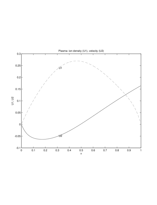
Figure 1:

6 Conclusion

After an application of PDAEs with a nonlinear convection term we first considered the determination of the time and spatial index of such systems. These were based on definitions given earlier in the literature, e.g. [14]. We reduced this problem to the question whether there is an inverse of some operator defined on a properly defined solution space. For the case of the plasma PDAE (a system with time index 1) this was shown in detail. In most practical applications, PDAEs have time index less than 3.
Then we studied the numerical solution of corresponding IBVPs by means of a finite difference splitting method familiar from the treatment of partial differential equations. Especially the convergence was considered for the case that both the time and space step sizes tend to zero. The main problem in these investigations is (in one space dimension) to handle the limit $h\to 0$ in relation to the time step size $\tau$. For fixed $h$ and $\tau\to 0$ this problem is easy. Some results concerning the problem when both $h$ and $\tau$ go to zero were given.
Finally, some results of a numerical solution of an IBVP from plasma physics were presented. This example is interesting because the PDAE which is nonlinear is a mixture of partial differential equations of parabolic, elliptic and hyperbolic type.

References

- [1] K.E. Brenan, S.L. Campbell, and L.R. Petzold. Numerical solution of initial-value problems in differential-algebraic equations. North-Holland Publ. Co., Amsterdam, 1989.
- [2] S. L. Campbell and W. Marszalek. ODE/DAE integrators and MOL problems. ICIAM 95 Minisymposium on MOL, 1995.
- [3] S.L. Campbell and W. Marszalek. The index of an infinite dimensional implicit system. Math. Mod. of Syst., 1(1):1–25, 1996.
- [4] S.L. Campbell and W. Marszalek. DAEs arising from traveling wave solutions of PDEs. J. Comput. Appl. Math., 82(1-2):41–58, 1997.
- [5] S. C. Cowin. Bone poroelasticity. Journ. of Biomechan., 32:217–238, 1999.
- [6] E. Detournay and H.-D. A. Cheng. Fundamentals of poroelasticity. In: Hudson, J. A. (Ed.), Comprehensive rock engineering: principles, practice and projects. Pergamon, Oxford, 1993.
- [7] R.K. Dodd, J.C. Eilbeck, J.D. Gibbon, and H.C. Morris. Solitons and nonlinear wave equations. Academic Press, New York, 1982.
- [8] M. Günther and Y. Wagner. Index concepts for linear mixed systems of differential-algebraic and hyperbolic-type equations. SIAM Journ. on Sci. and Statist. Comp., in press, 1999.
- [9] N.N. Janenko. Die Zwischenschrittmethode zur Lösung mehrdimensionaler Probleme der mathematischen Physik. Springer-Verlag, Berlin, 1969.
- [10] W. Lucht and K. Debrabant. Models of quasi-linear PDAEs with convection. Technical report, Martin-Luther-Universität Halle, Fachbereich Mathematik und Informatik, 2000.
- [11] W. Lucht and K. Strehmel. Discretization based indices for semilinear partial differential algebraic equations. Appl. Numer. Math., 28:371–386, 1998.
- [12] W. Lucht, K. Strehmel, and C. Eichler-Liebenow. Indexes and special discretization methods for linear partial differential algebraic equations. BIT, 39, No. 3:484–512, 1999.
- [13] W. Marszalek. Analysis of partial differential algebraic equations. PhD thesis, North Carolina State University, Raleigh, 1997.
- [14] W.S. Martinson and P.I. Barton. A differentiation index for partial differential equations. SIAM Journ. Sci. Comp., 21, no.6:2295–2315, 2000.