Magnetism of CuX${}_{2}$ frustrated chains (X = F, Cl, Br): the role of covalency

Abstract

Periodic and cluster density-functional theory (DFT) calculations, including DFT+$U$ and hybrid functionals, are applied to study magnetostructural correlations in spin-1/2 frustrated chain compounds CuX${}_{2}$: CuCl${}_{2}$, CuBr${}_{2}$, and a fictitious chain structure of CuF${}_{2}$. The nearest-neighbor and second-neighbor exchange integrals, $J_{1}$ and $J_{2}$, are evaluated as a function of the Cu–X–Cu bridging angle $\theta$ in the physically relevant range 80–110${}^{\circ}$. In the ionic CuF${}_{2}$, $J_{1}$ is ferromagnetic for $\theta\leq 100^{\circ}$. For larger angles, the antiferromagnetic superexchange contribution becomes dominant, in accord with the Goodenough-Kanamori-Anderson rules. However, both CuCl${}_{2}$ and CuBr${}_{2}$ feature ferromagnetic $J_{1}$ in the whole angular range studied. This surprising behavior is ascribed to the increased covalency in the Cl and Br compounds, which amplifies the contribution from Hund’s exchange on the ligand atoms and renders $J_{1}$ ferromagnetic. At the same time, the larger spatial extent of X orbitals enhances the antiferromagnetic $J_{2}$, which is realized via the long-range Cu–X–X–Cu paths. Both, periodic and cluster approaches supply a consistent description of the magnetic behavior which is in good agreement with the experimental data for CuCl${}_{2}$ and CuBr${}_{2}$. Thus, owing to their simplicity, cluster calculations have excellent potential to study magnetic correlations in more involved spin lattices and facilitate application of quantum-chemical methods.

I Introduction

Copper compounds have been extensively studied as spin-$\frac{1}{2}$ quantum magnets, material prototypes of quantum spin models. While local properties of these compounds are usually similar and involve nearly isotropic Heisenberg spins, the variability of the magnetic behavior stems from the unique structural diversity. Depending on the particular arrangement of the magnetic Cu${}^{2+}$ atoms and their ligands in the crystal structure, different spin lattices can be formed. Presently, experimental examples for many of simple lattice geometries, including the uniform chain,Stone et al. (2003); Lake et al. (2005) square lattice,Rønnow et al. (1999); *ronnow2001; Tsyrulin et al. (2009) Shastry-Sutherland lattice of orthogonal spin dimers,Miyahara and Ueda (2003); Takigawa et al. (2010) and kagomé lattice,Mendels and Bert (2010) are available and actively studied. Some of the copper compounds feature more complex spin latticesRüegg et al. (2007); Mentré et al. (2009); *tsirlin2010; Janson et al. (2012) that have not been anticipated in theoretical studies, yet trigger the theoretical researchLaflorencie and Mila (2011); Lavarélo et al. (2011) once relevant material prototypes are available.

Owing to the competition between ferromagnetic (FM) and antiferromagnetic (AFM) contributions to the exchange couplings, compounds of particular interest are those with M-X-M bridging angles close to 90${}^{\circ}$, with M being a transition metal and X being a ligand. Such geometries are realized in the quasi-1D cuprates featuring chains of edge-sharing CuO${}_{4}$ plaquettes, which represent a simple example of low-dimensional spin-1/2 magnetic materials. Independent of the sign of the nearest-neighbor (NN) coupling $J_{1}$, its competition with the sizeable AFM next-nearest-neighbor (NNN) coupling $J_{2}$ leads to magnetic frustration. Depending on the ratio $J_{2}/J_{1}$, such compounds exhibit exotic magnetic behavior like helical order,Mourigal et al. (2011) spin-Peierls transitionHase et al. (1993) or quantum critical behavior.Drechsler et al. (2007) The difficulties in the microscopic description of such compounds originate from ambiguities in the experimental estimates of the ratio $J_{2}/J_{1}$, leading to controversial modeling of the magnetic structure.Masuda et al. (2004); *FHC_LiCu2O2_chiT_CpT_NS_wrong_model_comment; *FHC_LiCu2O2_chiT_CpT_NS_wrong_model_reply Thus, the combination of different sets of experimental data with a careful theoretical analysis of the individual exchange pathways is of crucial importance for obtaining a precise microscopic magnetic model.

However, the search for new quantum magnets, as well as the work on existing materials, require not only the ability to estimate the couplings but also a solid understanding of the nexus between crystallographic features of the material and ensuing magnetic couplings. The Goodenough-Kanamori-Anderson (GKA)Goodenough (1955); *GKA_2; *GKA_3 rules are a generic and well-established paradigm that prescribes FM couplings for bridging angles close to 90${}^{\circ}$ and AFM couplings else, where the bridging angle refers to the M–X–M pathway. In Cu${}^{2+}$ oxides, generally the GKA rules successfully explain the crossover between the FM and AFM interactions for Cu–O–Cu angles close to 90${}^{\circ}$. The boundary between the FM and AFM regimes is usually within the range of $95-98^{\circ}$,Braden et al. (1996) but may considerably be altered by side groups and distortions.Geertsma and Khomskii (1996); Ruiz et al. (1997a); Lebernegg (2011)

In addition to Cu${}^{2+}$ oxides, the systems of interest include copper halides,Coldea et al. (1997); *coldea2001; Rüegg et al. (2003) carbodiimides,Zorko et al. (2011); *tsirlin2012 and other compound families. Although microscopic arguments behind the GKA rules should be also applicable to these non-oxide materials, the critical angles separating the FM and AFM regimes, as well as the role of the ligand in general, are still little explored. Moreover, the low number of experimentally studied compounds impedes a comprehensive experimental analysis available for oxides.

More and more, density functional theory (DFT) electronic structure calculations complement experimental studies and deliver accurate estimates of magnetic couplings.Lebernegg et al. (2011); Janson et al. (2010); Jeschke et al. (2011); Xiang and Whangbo (2007); Pickett (1997); Ku et al. (2002) They are especially well suited for the study of magnetostructural correlations, as both real and fictitious crystal structures can be considered in a calculation. However, in a periodic structure the effect of a single geometrical parameter is often difficult to elucidate, because different geometrical features are intertwined and evolve simultaneously upon the variation of an atomic position. Geometrical effects on the local magnetic coupling are better discerned in cluster models that represent a small group of magnetic atoms and, ideally, a single exchange pathway. Additional advantages of cluster models, owing to their low number of correlated atoms, are lower computational costs and, most important, their potential for the application of parameter-free wavefunction-based computational methods, i.e. in a strict sense $ab$ $initio$ calculations. By contrast, presently available band-structure methods for calculating strongly correlated compounds rely on empirical parameters and corrections where their choice is in general not unambiguous.Tsirlin et al. (2010b, 2011)

There have been several attempts to describe the local properties of solids with clusters especially in combination with $ab$ $initio$ quantum-chemical methods.Muñoz et al. (2002, 2005); Negodaev et al. (2010); Huang et al. (2011); Siurakshina et al. (2008) However, the construction of clusters is far from being trivial. On one side, to make the calculations computationally feasible, the number of quantum mechanically treated atoms has to be kept as small as possible. On the other side, accurate results require that these atoms experience the ”true” crystal potential. Usually, this is achieved by embedding the cluster into a cloud of point chargesMüller and Paulus (2012); Huang et al. (2011) and so called total ion potentials.Winter et al. (1987); de Graaf et al. (2002) But even for involved embeddings it was demonstrated, that the choice of the cluster may have significant effects on the results of the calculations and, thus, size-convergence has to be checked thoroughly.de Graaf et al. (2002)

Here, we study the effect of geometrical parameters on the magnetic exchange in Cu${}^{2+}$ halides. The family of halogen atoms spans a wide range of electronegativities, from the ultimately electronegative fluorine, forming strongly ionic Cu–F bonds, to chlorine and bromine that produce largely covalent compounds with Cu${}^{2+}$.van der Laan et al. (1981) Presently, we do not consider iodine because no Cu${}^{2+}$ iodides have been reported. In our modeling, we use the simplest possible periodic crystal structure of a CuX${}_{2}$ chain that enables the variation of the Cu–X–Cu bridging angle in a broad range. We further perform a comparative analysis for clusters and additionally consider the problem of long-range couplings. The evaluation of such couplings requires larger clusters, thus posing a difficulty for the cluster approach. The observed trends for the magnetic exchange as a function of the bridging angle are analyzed from the microscopic viewpoint, and reveal the crucial role of covalency that underlies salient differences between the ionic Cu${}^{2+}$ fluorides and largely covalent chlorides and bromides.

On the experimental side, the compounds and crystal structures under consideration are relevant to the CuCl${}_{2}$ and CuBr${}_{2}$ materials that show interesting examples of frustrated Heisenberg chains.Banks et al. (2009); Schmitt et al. (2009) At low temperatures, these halides form helical magnetic structures and demonstrate improper ferroelectricity along with the strong magnetoelectric coupling.Seki et al. (2010); Zhao et al. (2012)

The paper is organized as follows. In section II, the applied theoretical methods are presented. In the third section, the crystal structures of the CuX${}_{2}$ compounds are described and compared. In section IV, the results of periodic and cluster calculations are discussed and compared. Finally, the discussion, summary, and a short outlook are given in section V.

II Methods

The electronic structures of clusters and periodic systems were calculated with the full-potential local-orbital code fplo9.00-34.Koepernik and Eschrig (1999) For the scalar-relativistic calculations within the local density approximation (LDA), the Perdew-Wang parameterizationPerdew and Wang (1992) of the exchange-correlation potential was used together with a well converged mesh of up to 12$\times$12$\times$12 k-points for the periodic models.

The effects of strong electronic correlations were considered by mapping the LDA bands onto an effective tight-binding (TB) model. The transfer integrals $t_{i}$ of the TB-model are evaluated as nondiagonal elements between Wannier functions (WFs). For the clusters, the transfer integral corresponds to half of the energy difference of the magnetic orbitals.Hay et al. (1975) These transfer integrals $t_{i}$ are further introduced into the half-filled single-band Hubbard model $\hat{H}=\hat{H}_{TB}+U_{\text{eff}}\sum_{i}\hat{n}_{i\uparrow}\hat{n}_{i\downarrow}$ that is eventually reduced to the Heisenberg model for low-energy excitations,

$$\hat{H}=\sum_{\left\langle ij\right\rangle}J_{ij}\hat{S_{i}}\cdot\hat{S_{j}}$$ (1)

The reduction is well-justified in the strongly correlated limit $t_{i}\ll U_{\text{eff}}$, where $U_{\text{eff}}$ is the effective on-site Coulomb repulsion, which exceeds $t_{i}$ by at least an order of magnitude (see Table 1). This procedure yields AFM contributions to the exchange evaluated as $J_{i}^{\text{AFM}}=4t_{i}^{2}/U_{\text{eff}}$.

Alternatively, the full exchange couplings $J_{i}$, comprising FM and AFM contributions, can be derived from total energies of collinear magnetic arrangements evaluated in spin-polarized supercell calculations within the mean-field density functional theory (DFT)+$U$ formalism. We use a local spin-density approximation (LSDA)+$U$ scheme in combination with a unit cell quadrupled along the $b$ axis and a $k$-mesh of 64 points. The on-site repulsion and exchange amount to $U_{d}$ = 7$\pm$0.5 eV and $J_{d}$ = 1 eV, respectively. The same $U_{d}$ value is chosen for all CuX${}_{2}$ (X = F, Cl, Br) compounds to facilitate a comparison of the magnetic behavior. In section IV.5, however, it will be shown that $U_{d}$ has in fact no qualitative effect on the magnetic couplings of the CuX${}_{2}$ (X = F, Cl, Br) compounds. We applied the around mean field (AMF) as well as the fully localized limit (FLL) double counting corrections where both types where found to supply similar results. Thus, following the earlier studies of Cu${}^{2+}$ compounds,Schmitt et al. (2009); Lebernegg et al. (2011); Janson et al. (2010) the presented results are obtained within the AMF scheme.

For the clusters we used, in addition to the LSDA+$U$ method, the B3LYP hybrid functionalBecke (1993) with a 6-311G basis set. The B3LYP calculations were performed within the gaussian09 code.Frisch et al. The free parameter $\alpha$, indicating the admixture of exact exchange, was varied in the range between 0.15 and 0.25 to investigate its influence on the calculated exchange couplings.

III Crystal structures

The copper CuX${}_{2}$ dihalides feature isolated chains of edge-sharing CuX${}_{4}$ plaquettes.sup The chains of this type are the central building block of many well-studied cuprates such as CuGeO${}_{3}$ (Ref. Hase et al., 1993), Li${}_{2}$ZrCuO${}_{4}$ (Ref. Drechsler et al., 2007), and Li${}_{2}$CuO${}_{2}$ CuX${}_{2}$ halides are charge neutral, which makes them especially well suited for the modeling within the cluster approach.

CuBr${}_{2}$ crystallizes in the monoclinic space group $C2/m$ with $a$ = 14.728 Å, $b$ = 5.698 Å and $c$ = 8.067 Å, and $\beta$ = 115.15${}^{\circ}$ at room temperature.Oeckler and Simon (2000) The planar chains of edge-sharing CuBr${}_{4}$ plaquettes run along the $b$-axis (Fig. 1). The Cu–Br–Cu bridging angle $\theta$ amounts to 92.0${}^{\circ}$, the Cu–Br distance is 2.41 Å, while the distances between the neighboring chains amount to $d_{\parallel}$ = 3.82 Å and $d_{\perp}$ = 3.15 Å in the direction parallel to $c$ and perpendicular to the plaquette plane, respectively.

CuCl${}_{2}$ is isostructural to CuBr${}_{2}$ with the Cu–Cl distance of 2.26 Å and $\angle$(Cu–Cl–Cu) = 93.6${}^{\circ}$.Burns and Hawthorne (1993) The interchain separations amount to $d_{\parallel}$ = 3.73 Å and $d_{\perp}$ = 2.96 Å along the $c$ and $a$ directions, respectively.

CuF${}_{2}$ features a two-dimensional distorted version of the rutile structure, with corner-sharing CuF${}_{4}$ plaquettes forming a buckled square lattice.Burns and Hawthorne (1991) This atomic arrangement is very different from the chain structures of CuCl${}_{2}$ and CuBr${}_{2}$. For the sake of comparison with other Cu${}^{2+}$ halides, we constructed a fictitious one-dimensional structure of CuF${}_{2}$. The Cu–F distance of 1.91 Å was chosen to match the respective average bond length in the real CuF${}_{2}$ compound. The corresponding bridging angle, yielding a minimum in total energy, was determined to be 102${}^{\circ}$. Although this crystal structure remains hypothetical, it is likely metastable and could be formed in CuF${}_{2}$ under a strong tensile strain on an appropriate substrate.

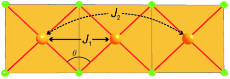
Figure 1: (Color online) Edge-sharing CuX${}_{4}$-plaquettes forming the magnetic chains in the CuX${}_{2}$ compounds. The chains, running along [010] are flat and lie in the $ab$ plane. The stacking of the planes is accompanied by a shift to match the monoclinic angle.sup The arrows indicate the nearest-neighbor and next-nearest-neighbor interaction pathways, and $\theta$ denotes the Cu-X-Cu bridging angle.

IV Results

IV.1 Band structure calculations

First, we consider magnetic couplings in the experimental crystal structures of CuCl${}_{2}$ and CuBr${}_{2}$, as well as in the relaxed structure of chain-like CuF${}_{2}$. The DFT calculations of the band structure and the density of states (DOS) of CuX${}_{2}$ (X = F, Cl, Br) compounds within the LDA yield a valence band width of 6–8 eV,sup in agreement with the experimental photoelectron spectra.van der Laan et al. (1981) The valence band complex becomes slightly narrower upon an increase in the ligand size, because the lower electronegativity of Cl and Br brings the respective $p$ states closer to the Cu $3d$ states, thus enhancing the hybridization and reducing the energy separation between the Cu and ligand orbitals. All the band structures feature a separated band crossing the Fermi level (Fig. 2). In the local-orbital representation visualized by WFs (Fig. 4), this band is formed by the antibonding $\sigma$*-combination of Cu $3d_{x^{2}-y^{2}}$ and X $p$ orbitals. The isolated half-filled band suffices for describing the magnetic properties and the low-lying magnetic excitations via the transfer integrals $t_{i}$ which are subsequently introduced into a Hubbard model. Ligand valence $p$-orbital contributions to the magnetic orbital, denoted as $\beta$ in Table 1, illustrate the increase in the metal–ligand hybridization from F to Br.

The dispersion calculated with the WF-based one-band TB model for CuBr${}_{2}$ is also shown in Fig. 2, and the leading transfer integrals together with the AFM contributions $J_{i}^{\text{AFM}}$ are given in Table 1. The evaluation of $J_{i}^{\text{AFM}}$ requires the value of $U_{\text{eff}}$, which is not known precisely. Here, we estimate $U_{\text{eff}}$ by comparing the transfer integral $t_{2}$ obtained from the TB analysis with the exchange coupling $J_{2}$ from the LSDA+$U$ calculations. While short-range couplings may involve large FM contributions, the long-range coupling $J_{2}$ should be primarily AFM. Therefore, $J_{2}^{\text{AFM}}=J_{2}$ in a good approximation, and $U_{\text{eff}}=4t_{2}^{2}/J_{2}$. This way, we find $U_{\text{eff}}=6$ eV for X = F, 4 eV for Cl, and 3 eV for Br. The reduction in $U_{\text{eff}}$ reflects the general trend of the enhanced Cu–X hybridization and covalency, because the $U_{\text{eff}}$ value pertains to the screened Coulomb repulsion in the mixed Cu–X band. The enhanced hybridization leads to a stronger screening, larger spatial extension and, thus, to the lower $U_{\text{eff}}$ values.

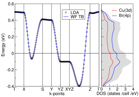
Figure 2: (Color online) Comparison of the calculated LDA band structure of CuBr${}_{2}$ and the band derived from a fit using an effective one-band tight-binding model based on Cu-centered Wannier functions (WF TB). The right plot shows the total density of states (DOS) together with the partial DOS of Cu(3$d$) and Br(4$p$) states. The Fermi level is at zero energy. Notation of $k$-points: $\Gamma=(000)$, X$=(\frac{\pi}{a}00)$, S$=(\frac{\pi}{a}\frac{\pi}{b}0)$, Y$=(0\frac{\pi}{b}0)$, YZ$=(0\frac{\pi}{b}\frac{\pi}{c})$, XYZ$=(\frac{\pi}{a}\frac{\pi}{b}\frac{\pi}{c})$, Z$=(00\frac{\pi}{c})$.

Table 1: Results for the experimental (X = Cl, Br) and hypothetical (X = F) structures of CuX${}_{2}$: the bridging angle $\theta$, the ligand contribution to the magnetic orbital $\beta$, transfer integrals $t_{i}$, AFM contributions to the exchange $J_{i}^{\text{AFM}}=4t_{i}^{2}/U_{\text{eff}}$, total exchange integrals $J_{i}$ from LSDA+$U$ calculations with $U_{d}=7\pm 0.5$ eV, and the effective on-site Coulomb repulsion $U_{\text{eff}}$ obtained by equilibration of $4t_{2}^{2}/U_{\text{eff}}$ (see text for details).

	$\theta$	$\beta$	$t_{1}$	$t_{2}$	$J^{AFM}_{1}$	$J^{AFM}_{2}$	$J_{1}$	$J_{2}$	$U_{\text{eff}}$
	(deg)		(meV)	(meV)	(meV)	(meV)	(meV)	(meV)	(eV)
CuBr${}_{2}$	92	0.28	47	136	2.5	21.0	$-8.8\pm 0.4$	$22.2\pm 3.4$	3.0
CuCl${}_{2}$	93.6	0.26	34	117	1.1	13.7	$-12.9\pm 0.9$	$13.4\pm 2.2$	4.0
CuF${}_{2}$	102	0.15	132	50	11.6	1.6	$5.4\pm 0.9$	$1.2\pm 0.2$	6.0

The estimates in Table 1 reveal two major differences between the ionic CuF${}_{2}$ and more covalent CuCl${}_{2}$ and CuBr${}_{2}$ compounds. First, the nearest-neighbor (NN) coupling $J_{1}$ is AFM in the fluoride, while FM in the chloride and bromide. Second, the AFM next-nearest-neighbor (NNN) coupling $J_{2}$ is enhanced upon increasing the covalency of the Cu–X bonds. In CuF${}_{2}$, this coupling is weak ($J_{2}\ll J_{1}$), whereas in the chloride and bromide $J_{2}\geq|J_{1}|$. The NNN coupling is amplified by the larger ligand size and the increased covalency. This coupling involves the long-range Cu–X–X–Cu pathway and requires a strong overlap between the ligand orbitals, which is possible for X = Cl and especially Br, while remaining weak for the smaller fluoride anion. The changes in the NN coupling seem to be well described by the GKA rules. Considering the trends for copper oxides,Braden et al. (1996) one expects FM $J_{1}$ for $\theta$ close to $90^{\circ}$, as in CuCl${}_{2}$ and CuBr${}_{2}$, and AFM $J_{1}$ for $\theta>98^{\circ}$, as in the chain-like structure of CuF${}_{2}$. Nevertheless, the covalency is also paramount for the sign of $J_{1}$, as shown by the magnetostructural correlations presented below (Sec. IV.2).

Finally, we briefly compare our DFT-based estimates of $J_{i}$ with the experiment. Because the chain-like polymorph of CuF${}_{2}$ has not been prepared experimentally, no comparison can be performed. The microscopic analysis of CuCl${}_{2}$ presented in Ref. Schmitt et al., 2009 shows reasonable agreement between the experimental ($J_{1}=-7.8$ meV, $J_{2}=11.6$ meV) and calculated ($J_{1}=-12.9\pm 0.9$ meV, $J_{2}=13.4\pm 2.2$ meV) values. The same is true for CuBr${}_{2}$, where we evaluated the intrachain couplings as $J_{1}=-8.8\pm 0.4$ meV, $J_{2}=22.2\pm 3.4$ meV which compare well with recently published experimental data $J_{1}=-11.0\pm 1.6$ meV, $J_{2}=31.0$ meV.Lee et al. (2012) Moreover, our calculations reveal significantly lower deviations from experiment than those supplied in Ref. Lee et al., 2012.

Puzzled by the origin of the discrepancy between our values for $J_{1}$ and $J_{2}$ and the published calculational results for CuBr${}_{2}$,Lee et al. (2012) we repeated the DFT+$U$ calculations for CuBr${}_{2}$ as well as CuCl${}_{2}$ with the code vaspKresse and Furthmüller (1996a); *vasp2 and the same computational parameters as used in Ref. Lee et al., 2012. For the parameters $U_{d}$ and $J_{d}$, we adopted 8 eV and 1 eV, respectively, which corresponds to the effective $U\!=U_{d}\!-\!J_{d}\!=\!7$ eV in Refs. Lee et al., 2012. For the GGA+$U$ calculations, we used again a unit cell quadrupled along the $b$ axis and the $k$-mesh of 64 points. The resulting $J_{1}$ and $J_{2}$ values generally agree with the published values,Banks et al. (2009); Lee et al. (2012) except for $J_{1}$ in CuBr${}_{2}$, for which we obtain only half of the value provided in Ref. Lee et al., 2012. The agreement with the experimental data can be improved by increasing the $U_{d}$ value. In particular, $U_{d}\!=\!12$ eV yields $J_{1}\!=\!-95$ K and $J_{2}$ = 113 K for CuCl${}_{2}$ and $J_{1}\!=\!-124$ K and $J_{2}$ = 357 K for CuBr${}_{2}$, very close to the experimental estimates.Schmitt et al. (2009); Lee et al. (2012) This $U_{d}$ value is significantly higher than the $U_{d}=7$ eV we used in our fplo9.00-34 calculations. There are basically two reasons for the large difference: The first reason are the different basis sets of fplo9.00-34 and vasp, implementing local orbitals and projected augmented waves,Blöchl (1994); *paw2 respectively, which crucially affect the local quantity $U_{d}$. Second, we used an around mean field double counting correction (DCC) while a fully localized limit DCC, which is always used in vasp, requires larger $U_{d}$ values.Tsirlin and Rosner (2010)

IV.2 Variation of the bridging angle

To establish magnetostructural correlations in CuX${}_{2}$ halides, we systematically vary the bridging angle $\theta$ and evaluate the NN coupling $J_{1}$. Since the Cu–Cu distance and two Cu–X distances form a triangle with $\theta$ being one of its angles, the change in $\theta$ alters either the Cu–Cu distance, or the Cu–X distance, or both. We compared different flavors of varying $\theta$: i) the Cu-Cu distance is varied, while the X position is subsequently optimized to yield the equilibrium Cu–X distance and $\theta$; ii) the Cu-Cu distance is fixed, while the Cu–X distance is varied; and iii) the Cu–X distance is fixed, while the Cu–Cu distance is varied. For all three cases, we evaluated $J_{1}$ as a function of the Cu–X–Cu angle. Fig. 3 shows on the example of CuCl${}_{2}$ that despite minor numerical differences, all three methods conform well to each other. Additionally, we studied the influence of $U_{d}$ by varying it in the wide range of 4–9 eV. This causes a shift of the curves along the vertical axis, but the qualitative behavior of $J_{1}$ versus the Cu-X-Cu angle is retained.sup

Remarkably, $J_{1}$ reaches its minimum absolute value at around $\theta=100^{\circ}$ and becomes strongly FM at large bridging angles (Fig. 3). This result is robust with respect to the particular procedure of varying $\theta$. To better understand the microscopic origin of this peculiar behavior, we performed similar calculations for CuF${}_{2}$ and CuBr${}_{2}$. As different procedures of varying $\theta$ arrive at similar results, we fixed the Cu–X distance for each ligand and achieved different $\theta$ values by adjusting the Cu–Cu distance, only.

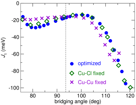
Figure 3: (Color online) $J_{1}$ of CuCl${}_{2}$ as function of the bridging angles where different structural parameters are fixed: i) the Cu-Cu distance is varied, while the X position is subsequently optimized to yield the equilibrium Cu–X distance and $\theta$; ii) the Cu-Cu distance is fixed, while the Cu–X distance is varied; and iii) the Cu–X distance is fixed, while the Cu–Cu distance is varied. The dashed vertical line indicates the experimental bridging angle.

Similar to our results for the fixed geometries (Table 1), magnetostructural correlations for $J_{1}$ (Fig. 4) reveal a large difference between the ionic CuF${}_{2}$ and covalent CuCl${}_{2}$ and CuBr${}_{2}$. In CuF${}_{2}$, $J_{1}$ follows the anticipated behavior with the FM-to-AFM crossover at $\theta\simeq 100^{\circ}$. However, the covalent compounds always show FM $J_{1}$, with a maximum (i.e., the minimum in the absolute value) at $\theta\!=\!100\!-\!105^{\circ}$ and the enhanced FM character at even larger bridging angles. This trend persists up to at least $\theta=120^{\circ}$ (Fig. 3).

The effect of strongly FM $J_{1}$ in CuCl${}_{2}$ and CuBr${}_{2}$ can be explained by considering individual contributions to the exchange. The AFM contribution $J_{1}^{\text{AFM}}$ arises from the electron hopping between the Cu sites. The hopping probability measured by the transfer integral $t_{1}$ critically depends on the Cu–X–Cu bridging angle. In a simple ionic picture, the transfer is maximal at $\theta=180^{\circ}$ (singly bridged) and approaches zero at $\theta=90^{\circ}$, thus providing the microscopic reasoning behind the GKA rules. This anticipated trend is indeed shown by CuF${}_{2}$, where $J_{1}^{\text{AFM}}=4t_{1}^{2}/U_{\text{eff}}$ increases above $\theta=90^{\circ}$ and underlies the increase in $J_{1}$. However, the covalent CuX${}_{2}$ halides show qualitatively different behavior with the very low (and decreasing) $t_{1}$ and $J_{1}^{\text{AFM}}$ up to at least $\theta=110^{\circ}$. This result implies that the large contribution of the ligand states in a covalent compound has also a strong influence on the Cu–X–Cu hopping process and alters the anticipated trend for the AFM exchange.

The FM contribution $J_{1}^{\text{FM}}$ can be evaluated as $J_{1}-J_{1}^{\text{AFM}}$, where we use $J_{1}$ from the LSDA+$U$ calculation and $J_{1}^{\text{AFM}}=4t_{1}^{2}/U_{\text{eff}}$ from the TB analysis. Microscopically, $J_{1}^{\text{FM}}$ originates from the Hund’s coupling on the ligand siteMazurenko et al. (2007) and/or from the FM coupling between the Cu $3d$ and ligand $p$ states.Nishimoto et al. (2012); *kuzian2012 Regarding the former mechanism,Mazurenko et al. (2007) a simple model expression reads as $J_{1}^{\text{FM}}=-\beta^{4}J_{H}$, where $\beta$ is the ligand’s contribution to the Cu-centered magnetic orbital, and $J_{H}$ is the (effective) Hund’s coupling on the ligand. Even though this expression is derived for $\theta=90^{\circ}$, our data obtained for different $\theta$ values are well understood in terms of the variable $\beta$ (see bottom panels of Fig. 4). The increase in the bridging angle leads to larger $\beta$, thus enhancing $J_{1}^{\text{FM}}$. Since $\beta$ enters $J_{1}^{\text{FM}}$ as $\beta^{4}$, its effect should be dominant over any other contributions, such as slight variations of $J_{H}$. The increase in $\beta$ also explains the increasing FM contribution at low $\theta$ (Fig. 4).

In contrast to the covalent chloride and bromide, the ionic CuF${}_{2}$ shows only a minor FM contribution owing to the very low $\beta$. We also tried to artificially enhance $\beta$ by reducing the Cu–F bonding distance down to 1.60 Å. For bridging angles larger than 100${}^{\circ}$ the AFM coupling becomes twice as large as for the Cu–F distance of 1.91 Å and for angles smaller than 80${}^{\circ}$ the model compound becomes also AFM. The FM coupling strength about 90${}^{\circ}$ is almost unaffected. This indicates the robust ionic nature of Cu–F bonds. The reduction in the Cu–F distance increases the electron transfer without changing the hybridization, hence $J_{1}^{\text{AFM}}$ is increased, while $J_{1}^{\text{FM}}$ remains weak.

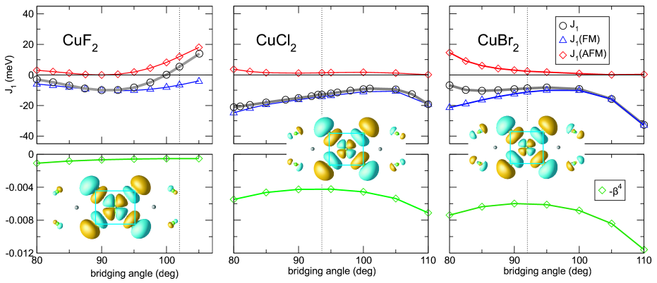
Figure 4: (Color online) Magnetostructural correlations for the CuX${}_{2}$ halides (the Cu–X distance is fixed, the Cu–Cu distance is variable). The upper panels show the total exchange $J_{1}$ (LSDA+$U$, $U_{d}=7$ eV) along with $J_{1}^{\text{AFM}}=4t_{1}^{2}/U_{\text{eff}}$ and $J_{1}^{\text{FM}}=J_{1}-J_{1}^{\text{AFM}}$. The bottom panels show $\beta^{4}$, where $\beta$ is the ligand’s contribution to the Cu-based magnetic orbital. The WFs for the experimental (relaxed) geometries are shown as insets.

IV.3 Cluster models

In a periodic calculation, the variation of structural parameters, such as bond lengths and angles, is generally challenging: the high symmetry couples the structural parameters to each other. As a result, changing a single parameter is often impossible without affecting the other parameters. The cluster models are more flexible and may allow for an independent variation of individual bond lengths and angles. This property renders the clusters as an excellent playground to study the magnetostructural correlations.

Before discussing the intrachain couplings using a combination of periodic and cluster models, we first want to demonstrate how cluster models for the three Cu dihalide compounds are constructed. Since the chains are spatially well-separated from each other, we can consider segments of a chain, with the terminal Li atoms keeping the electroneutrality (Fig. 5). No additional point charges are required, so that the clusters are kept as simple as possible.

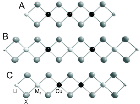
Figure 5: Three examples of model clusters: Cu${}_{3}$ trimer cluster as the minimal cluster for the evaluation of $J_{1}$ and $J_{2}$ (A); the pentamer cluster for calculating $J_{2}$, with only two Cu${}^{2+}$ and three substituted non-magnetic ions (B); and the tetramer cluster for calculating $J_{1}$ with two magnetic Cu and two nonmagnetic $M_{S}$ centers (C).

First, the effect of the chain length on $J_{1}$, $J_{2}$ and the ratio $-J_{2}/J_{1}$ is investigated (Fig. 6). For all three compounds, small clusters, such as dimers or trimers, are insufficient for describing the magnetic properties. The convergence with respect to the cluster size is different for different compounds (e.g., the ionic CuF${}_{2}$ demonstrates the slowest size convergence). To ensure a meaningful comparison with the periodic model or the experimental data, the convergence with respect to the cluster size has to be carefully checked.

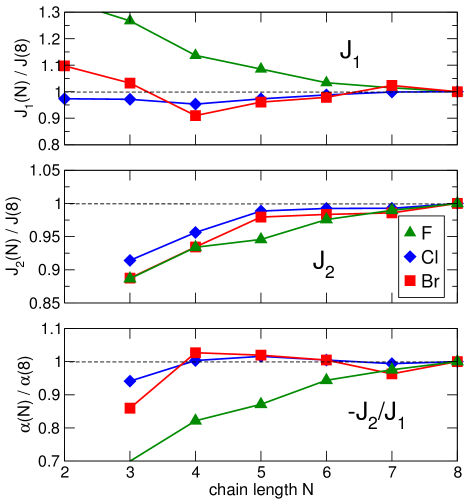
Figure 6: (Color online) $J_{1}(N)/J_{1}(N\!=\!8)$, $J_{2}(N)/J_{2}(N\!=\!8)$ and $\alpha(N)/\alpha(N\!=\!8)$ as a function of the chain length $N$. The bridging angle is fixed to the experimental (CuCl${}_{2}$ and CuBr${}_{2}$) and optimized (CuF${}_{2}$) values, respectively. For $J_{2}$ and $-J_{2}/J_{1}$, the minimal number of Cu-centers amounts to three. The exchange couplings are calculated with the LSDA+$U$ method with $U_{d}$ = 7 eV.

On the other hand, a large number of correlated centers requires a large number of spin configurations to estimate exchange couplings. While larger clusters are still feasible for DFT, they may pose a problem for advanced ab initio quantum-chemical methods. Therefore, we attempted to reduce the number of correlated Cu${}^{2+}$ ions by substituting them by formally nonmagnetic Mg${}^{2+}$ and Zn${}^{2+}$ ions (Fig. 5). Even with this minimum number of correlated centers, deviations below 10% to the size-converged Cu${}_{8}$ octamer cluster are obtained for the Cu–Br (Fig. 7) and also for the Cu–Cl clusters. In case of Cu-F, where convergence is reached at larger cluster size, at least four correlated centers are required to reduce the deviations down to that level.

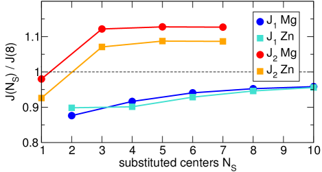
Figure 7: (Color online) $J_{1}$ and $J_{2}$ of the Cu-Br clusters calculated with clusters containing two correlated and N${}_{S}$ uncorrelated Mg${}^{2+}$ or Zn${}^{2+}$ centers. The bridging angle is fixed to the experimental value. The resulting exchange integrals are normalized to that for the Cu${}_{8}$-octamer cluster. For the calculations, the LSDA+$U$ method is used with $U_{d}$ = 7 eV.

Similar results, as for the $J$’s, concerning size convergence and substitutions are obtained for the NN and NNN transfers, $t_{1}$ and $t_{2}$, calculated in LDA. These results show that the simple clusters suffice for describing the intrachain physics of these compounds and that the problem of appropriately embedding the clusters may be at least partially bypassed by increasing the cluster size and substituting part of the correlated centers with weakly correlated ions.

IV.4 Cluster versus periodic models

In the following, both cluster and periodic models will be used for calculating $J_{2}$ and the $-J_{2}/J_{1}$ ratio, as well as the transfer integrals $t_{i}$ of the Cu dihalides. The comparison of periodic and cluster models for a broad range of bridging angles allows to exclude an accidental agreement between both models, which can be realized in a specific geometry by appropriately choosing the chain length, substitutions, and the termination of the cluster. However, when the cluster is prepared in such a way, the good agreement with the periodic model would be lost by varying the geometrical parameters.

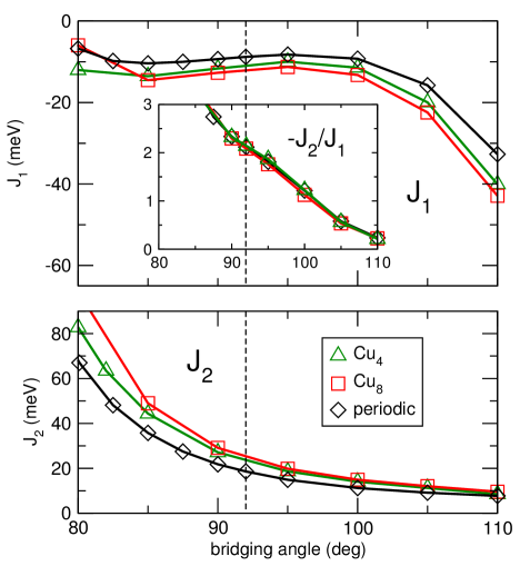
Figure 8: (Color online) CuBr${}_{2}$: exchange integrals $J_{1}$ and $J_{2}$ as a function of the bridging angle. A periodic as well as two different cluster models (Cu${}_{4}$ and Cu${}_{8}$) were used. The inset shows the ratio $-J_{2}/J_{1}$. The dashed vertical line indicates the experimental bridging angle of 92${}^{\circ}$. For the calculations, the LSDA+$U$ method is used with $U_{d}$ = 7 eV.

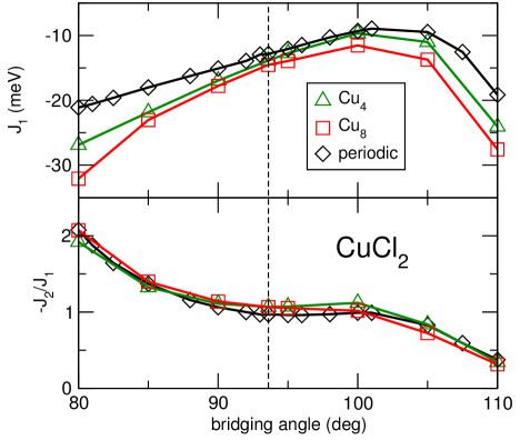
Figure 9: (Color online) Exchange integrals $J_{1}$ and the ratio $-J_{2}/J_{1}$ of CuCl${}_{2}$ as a function of the bridging angle calculated with a periodic and two cluster models. The dashed vertical line indicates the experimental bridging angle of 93.6${}^{\circ}$. For the CuF${}_{2}$ data, see supplementary information. For the calculations, the LSDA+$U$ method is used with $U_{d}$ = 7 eV.

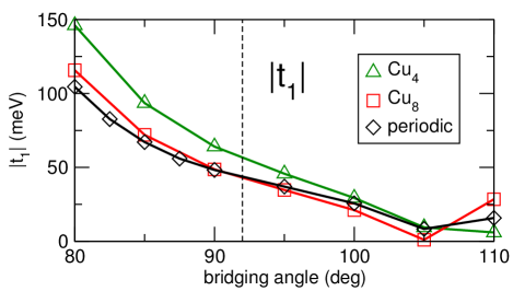
Figure 10: (Color online) CuBr${}_{2}$: the nearest-neighbor transfer integral $t_{1}$ as a function of the bridging angle calculated with a periodic as well as two cluster models (Cu${}_{4}$ and Cu${}_{8}$).

The exchange integrals as well as the $-J_{2}/J_{1}$ ratio versus the bridging angles are depicted in Figs. 8 and 9 for CuBr${}_{2}$ and CuCl${}_{2}$, respectively. A comparison of the nearest-neighbor transfer integral $t_{1}$ of CuBr${}_{2}$, calculated with cluster and periodic models, is shown in Fig. 10. The clusters can reproduce the results of band structure calculations over the whole range of bridging angles, thus justifying the construction of the clusters. In the $-J_{2}/J_{1}$ ratio, which governs the magnetic ground state, the deviations between the cluster and periodic models are compensated to a large degree.

In CuF${}_{2}$, the deviations between $J_{1}$ and $J_{2}$ obtained in the cluster and periodic models, respectively, are also compensated in the ratio $-J_{2}/J_{1}$, except for the smallest bridging angles.sup The singularity in $-J_{2}/J_{1}$ at about 100${}^{\circ}$ arises from the crossover between the FM and the AFM $J_{1}$.

These results show that well-controlled cluster models are capable of describing local properties of ionic as well as strongly covalent solids, whereas the good agreement with band structure calculations is not accidental or artificial. Finally, the results demonstrate that superexchange and magnetic coupling in insulators are relatively short-range effects even for strongly covalent compounds.

IV.5 LSDA+$U$ vs. hybrid functionals

A common problem of DFT-based approaches applied to strongly correlated electrons is the ambiguous choice of empirical parameters and corrections that are required to mimic many-body effects, e.g., in the mean-field DFT+$U$ approach. Hybrid functionals represent an alternative, although still empirical, way of simulating the effect of strong electron correlations within DFT. In this way, the non-local exact exchange is mixed with the local LDA or GGA exchange, while the mixing parameter $\alpha$ is typically the only free parameter. In contrast to DFT+$U$, hybrid functionals are more robust with respect to the adjustable parameters, and the constant value of $\alpha=0.20$ or $\alpha=0.25$ can be used in a rather general fashion. Additionally, the exact exchange correction is generally applied to all orbitals while in DFT+$U$ the corrections are applied to a certain set of orbitals which are assumed to be the strongly correlated ones.

In this study, we apply the B3LYP functional on dimer models and vary $\alpha$ between 0.15 and 0.25 ($\alpha=0.20$ corresponds to the standard B3LYP functional as implemented in gaussian). Although we pointed out that dimer models are too small for calculating $J_{1}$ in quantitative agreement with the periodic model, they are well suited for comparing the different DFT methods and parameter sets. Despite substantially different treatment of many-body effects in DFT+$U$ and hybrid functionals, the resulting exchange integrals of all three CuX${}_{2}$ compounds are quite similar (Fig. 11). Thus, the B3LYP calculations confirm the LSDA+$U$ results, justify the choice of the free parameters in the latter approach and demonstrate that the unusual FM $J_{1}$ coupling of CuCl${}_{2}$ and CuBr${}_{2}$ is not an artifact of a certain method. Despite the fact that B3LYP was originally constructed to reproduce the thermodynamical data for small molecules, it provides meaningful results for strongly correlated systems such as CuX${}_{2}$, in line with the earlier studies.Ruiz et al. (1997b); Muñoz et al. (2002); Tabookht et al. (2010) Moreover, the calculated exchange integrals are robust with respect to $\alpha$: the exchange integrals are rather insensitive to the choice of this parameter.

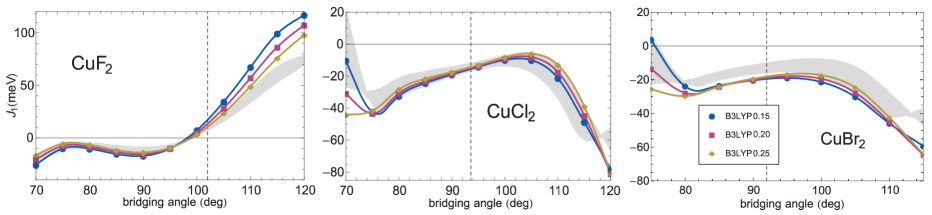
Figure 11: (Color online) The exchange integral $J_{1}$ of the CuX${}_{2}$ (X = F, Cl, Br) compounds as a function of the bridging angle. The calculations are done for a dimer model with LSDA+$U$ and $U_{d}=7\pm 1$ eV (grey area), and with the B3LYP functional ($\alpha=0.15-0.25$).

V Discussion and Summary

Our study of magnetostructural correlations in the CuX${}_{2}$ halides reveals the crucial role of the ligand in magnetic exchange. Its effect is two-fold: First, the larger size of Cl and Br is responsible for the enhanced NNN coupling $J_{2}$ that is assisted by the sizable overlap of ligand $p$ orbitals along the Cu–X–X–Cu pathway. Second, the covalent nature of the Cu–Cl and Cu–Br bonds underlies the large ligand contribution to the magnetic orbitals and, consequently, the strong FM nearest-neighbor (NN) coupling $J_{1}$ in the broad range of bridging angles which could be ascribed to Hund’s exchange on the ligand site. The tendency of covalent Cu${}^{2+}$ halides to exhibit FM exchange along the Cu–X–Cu pathways can be illustrated but also challenged by several experimental observations. It should be emphasized that ferromagnetic NN coupling requires not only sizeable ferromagnetic contributions but also small transfer integrals as were found for CuCl${}_{2}$ and CuBr${}_{2}$. Otherwise, the AFM contributions will outweigh the FM terms even for covalent compounds.

Experimental data for Cu${}^{2+}$ chlorides and bromides indeed show the robust FM NN coupling for the bridging angles below $90^{\circ}$. While the $\theta<90^{\circ}$ regime is not typical for the ionic oxides and fluorides, it is abundant in covalent systems and observed, e.g., in Cu-based FM spin chains.Willet and Landee (1981); *devries1987 The FM nature of the NN coupling at $\theta\!=\!90\!-\!95^{\circ}$ is evidenced by CuCl${}_{2}$ and CuBr${}_{2}$ themselves.Banks et al. (2009); Schmitt et al. (2009); Zhao et al. (2012); Lee et al. (2012) However, larger $\theta$ values are less common and require geometries other than the edge-sharing CuX${}_{2}$ chains considered in the present study.

The angles of $\theta>95^{\circ}$ are only found in edge-sharing dimers and corner-sharing chains. Moreover, the respective experimental situation is rather incoherent. In (CuBr)LaNb${}_{2}$O${}_{7}$ and (CuCl)LaTa${}_{2}$O${}_{7}$, the corner-sharing geometry with $\theta>100^{\circ}$ indeed leads to the FM exchange, although with a tendency towards AFM exchange at $\theta\geq 108-109^{\circ}$ (Refs. Tsirlin et al., 2012b, c). By contrast, the Cu${}_{2}$Cl${}_{6}$ dimers may reveal the AFM exchange even at $\theta\simeq 95.5^{\circ}$, as in LiCuCl${}_{3}\cdot 2$H${}_{2}$O (Ref. Abrahams and Williams, 1963) or TlCuCl${}_{3}$ and KCuCl${}_{3}$ (Ref. Shiramura et al., 1997) where the latter exhibit transfer integrals that are 3.5 times larger as that in CuCl${}_{2}$. On the other hand, similar Cu${}_{2}$Cl${}_{6}$ dimers with the same bridging angle of $\theta\simeq 95.5^{\circ}$ in the spin-ladder compound IPA-CuCl${}_{3}$ feature the sizable FM intradimer coupling.Masuda et al. (2006)

These experimental examples show that the bridging angle $\theta$ may not be the single geometrical parameter determining the Cu–X–Cu superexchange. Details of the atomic arrangement are important even for Cu${}^{2+}$ oxides,Ruiz et al. (1997b); *ruiz97_2 whereas in more covalent systems this effect is likely exaggerated because interactions involve specific orbitals, so that each bond determines the orientation of other bonds around the same atom. We have pointed out, that such magnetostructural correlations, essential for understanding the magnetic behavior and for the search of new interesting materials, can nicely be investigated with cluster models. In particular in case of intricate crystal structures clusters enable studying effects of each structural parameters separately, while for periodic models only a set of parameters can be modified at once.

On a more general side, our results identify the Cu–X–Cu pathways as the leading mechanism of the short-range exchange in Cu${}^{2+}$ halides. The fact that the magnetostructural correlations weakly depend on the procedure of varying $\theta$ (Fig. 3) entails the minor role of direct Cu–Cu interactions, because the coupling always evolves in a similar fashion, no matter whether the Cu–Cu distance is fixed or varied. Therefore, the nature of the ligand is of crucial importance, and affects the Cu–X–Cu hopping along with the FM contribution, presumably related to the Hund’s coupling on the ligand site.Mazurenko et al. (2007) In ionic systems, the nearest neighbor hopping increases with the bridging angle and dominates over the small FM contributions, thus leading to the conventional GKA behavior. However, the GKA behavior may be strongly altered in covalent compounds, as shown by our study and previously argued in model studies on the effect of side groups and distortions.Geertsma and Khomskii (1996); Lebernegg (2011); Ruiz et al. (1997b)

From the computational perspective, magnetic modeling of chlorides and bromides is generally challenging. Although these compounds are still deep in the insulating regime, far from the Mott transition ($t_{i}\ll U_{\text{eff}}$, see Table 1), the sizable hybridization of ligand states with correlated Cu $3d$ orbitals challenges the DFT+$U$ approach, with correlation effects restricted to the $d$ states. The microscopic evaluation of magnetic couplings in Cu${}^{2+}$ chlorides and bromides indeed leads to large uncertainties.Tsirlin et al. (2012c); Foyevtsova et al. (2011) Hybrid functionals, on the other hand, tend to overestimate magnetic exchange couplingsMuñoz et al. (2002) and provide a working, but empirical solution to the problem of strongly correlated electronic systems. This calls for the development and application of alternative techniques, as for instance ab initio quantum-chemical calculations, appropriately accounting for strong electron correlations. Since the wavefunction-based quantum-chemical calculations are presently restricted to finite systems, they require the construction of appropriate clusters. This task has been successfully accomplished in our work. We have demonstrated that relatively small clusters with a low number of correlated centers are capable of reproducing the results obtained for periodic systems, and provide adequate estimates of the magnetic exchange even for the long-range Cu–X–X–Cu interactions.

In summary, we have studied magnetostructural correlations in the family of CuX${}_{2}$ halides with X = F, Cl, and Br. Our results show substantial differences between the ionic CuF${}_{2}$ and largely covalent CuCl${}_{2}$ and CuBr${}_{2}$. The fluoride compound behaves similar to Cu${}^{2+}$ oxides, and shows weak FM exchange at the bridging angles close to $\theta=90^{\circ}$ along with the AFM exchange at $\theta\geq 100^{\circ}$. Going from F to Cl and Br leads to two major changes: i) the larger size of the ligand amplifies the AFM next-nearest-neighbor coupling $J_{2}$; ii) the increased covalency of the Cu–X bonds results in the strong mixing between the Cu $3d$ and ligand $p$ states, and enhances the FM contribution to the short-range nearest-neighbor coupling $J_{1}$. We have constructed cluster models which, first, supplied an excellent description of local properties of the solids. Second, they turned out as highly valuable tool for investigating magnetostructural correlations, e.g., they could be instrumental in the microscopic analysis of the covalent Cu${}^{2+}$ chlorides and bromides with interesting but still barely explored magnetism. Finally, they seem to be a viable approach to parameter-free quantum-chemical calculations of strongly correlated solids.

VI Acknowledgements

We acknowledge valuable discussions with O. K. Anderson and P. Blaha. S. L. acknowledges the funding from the Austrian Fonds zur Förderung der wissenschaftlichen Forschung (FWF). A.T. was partly supported by the Mobilitas grant of the ESF.

Supporting Material

(Color online) Crystal structure of the CuX${}_{2}$ (X = F, Cl, Br) compounds. Edge-sharing CuX${}_{4}$ plaquettes form planar chains running along the b-axis. For CuF${}_{2}$, this is a fictitious structure which is introduced in order to investigate the effects of different ligand size on the intrachain magnetic couplings. Real CuF${}_{2}$ features a 2-dimensional structure of corner-sharing CuF${}_{4}$-plaquettes that would be inappropriate for such purposes. $t_{1}$ and $t_{2}$ denote nearest-neighbor and next-nearest-neighbor intrachain hopping, respectively. $t_{i}c$ is the interchain hopping which is expected to have a negligible effect on the intrachain couplings.

References

- Stone et al. (2003) M. B. Stone, D. H. Reich, C. Broholm, K. Lefmann, C. Rischel, C. P. Landee, and M. M. Turnbull, Phys. Rev. Lett. 91, 037205 (2003).
- Lake et al. (2005) B. Lake, D. A. Tennant, C. D. Frost, and S. E. Nagler, Nature Mater. 4, 329 (2005).
- Rønnow et al. (1999) H. M. Rønnow, D. F. McMorrow, and A. Harrison, Phys. Rev. Lett. 82, 3152 (1999).
- Rønnow et al. (2001) H. M. Rønnow, D. F. McMorrow, R. Coldea, A. Harrison, I. D. Youngson, T. G. Perring, G. Aeppli, O. Syljuasen, K. Lefmann, and C. Rischel, Phys. Rev. Lett. 87, 037202 (2001).
- Tsyrulin et al. (2009) N. Tsyrulin, T. Pardini, R. R. P. Singh, F. Xiao, P. Link, A. Schneidewind, A. Hiess, C. P. Landee, M. M. Turnbull, and M. Kenzelmann, Phys. Rev. Lett. 102, 197201 (2009).
- Miyahara and Ueda (2003) S. Miyahara and K. Ueda, J. Phys.: Cond. Matter 15, R327 (2003).
- Takigawa et al. (2010) M. Takigawa, T. Waki, M. Horvatić, and C. Berthier, J. Phys. Soc. Jpn. 79, 011005 (2010).
- Mendels and Bert (2010) P. Mendels and F. Bert, J. Phys. Soc. Jpn. 79, 011001 (2010).
- Rüegg et al. (2007) C. Rüegg, D. F. McMorrow, B. Normand, H. M. Rønnow, S. E. Sebastian, I. R. Fisher, C. D. Batista, S. N. Gvasaliya, C. Niedermayer, and J. Stahn, Phys. Rev. Lett. 98, 017202 (2007).
- Mentré et al. (2009) O. Mentré, E. Janod, P. Rabu, M. Hennion, F. Leclercq-Hugeux, J. Kang, C. Lee, M.-H. Whangbo, and S. Petit, Phys. Rev. B 80, 180413(R) (2009).
- Tsirlin et al. (2010a) A. A. Tsirlin, I. Rousochatzakis, D. Kasinathan, O. Janson, R. Nath, F. Weickert, C. Geibel, A. M. Läuchli, and H. Rosner, Phys. Rev. B 82, 144426 (2010a).
- Janson et al. (2012) O. Janson, I. Rousochatzakis, A. A. Tsirlin, J. Richter, Y. Skourski, and H. Rosner, Phys. Rev. B 85, 064404 (2012).
- Laflorencie and Mila (2011) N. Laflorencie and F. Mila, Phys. Rev. Lett. 107, 037203 (2011).
- Lavarélo et al. (2011) A. Lavarélo, G. Roux, and N. Laflorencie, Phys. Rev. B 84, 144407 (2011).
- Mourigal et al. (2011) M. Mourigal, M. Enderle, R. K. Kremer, J. M. Law, and B. Fåk, Phys. Rev. B 83, 100409 (2011).
- Hase et al. (1993) M. Hase, I. Terasaki, and K. Uchinokura, Phys. Rev. Lett. 70, 3651 (1993).
- Drechsler et al. (2007) S.-L. Drechsler, O. Volkova, A. N. Vasiliev, N. Tristan, J. Richter, M. Schmitt, H. Rosner, J. Málek, R. Klingeler, A. A. Zvyagin, and B. Büchner, Phys. Rev. Lett. 98, 077202 (2007).
- Note (1) The same value of specific physical properties such as propagation vectors or spin gaps can be realized in different parts of the phase-diagram. To illustrate this effect, we consider an AFM and \tmspace+.1667em=\tmspace+.1667em0. In this case, the model is reduced to a uniform Heisenberg chain. In the other limit, \tmspace+.1667em=\tmspace+.1667em0 with an AFM , the system reduces to two decoupled uniform Heisenberg chains. Although the ratios are very different for these two cases, the physics is the same.
- Masuda et al. (2004) T. Masuda, A. Zheludev, A. Bush, M. Markina, and A. Vasiliev, Phys. Rev. Lett. 92, 177201 (2004).
- Drechsler et al. (2005) S.-L. Drechsler, J. Málek, J. Richter, A. S. Moskvin, A. A. Gippius, and H. Rosner, Phys. Rev. Lett. 94, 039705 (2005).
- Masuda et al. (2005) T. Masuda, A. Zheludev, A. Bush, M. Markina, and A. Vasiliev, Phys. Rev. Lett. 94, 039706 (2005).
- Goodenough (1955) J. B. Goodenough, Phys. Rev. 100, 564 (1955).
- Kanamori (1959) J. Kanamori, J. Phys. Chem. Solids 10, 87 (1959).
- Anderson (1963) P. W. Anderson, Solid State Phys. 14, 99 (1963).
- Braden et al. (1996) M. Braden, G. Wilkendorf, J. Lorenzana, M. Aïn, G. J. McIntyre, M. Behruzi, G. Heger, G. Dhalenne, and A. Revcolevschi, Phys. Rev. B 54, 1105 (1996).
- Geertsma and Khomskii (1996) W. Geertsma and D. Khomskii, Phys. Rev. B 54, 3011 (1996).
- Ruiz et al. (1997a) E. Ruiz, P. Alemany, S. Alvarez, and J. Cano, Inorg. Chem. 36, 3683 (1997a).
- Lebernegg (2011) S. Lebernegg, Croat. Chem. Acta 84, 505 (2011).
- Coldea et al. (1997) R. Coldea, D. A. Tennant, R. A. Cowley, D. F. McMorrow, B. Dorner, and Z. Tylczynski, Phys. Rev. Lett. 79, 151 (1997).
- Coldea et al. (2001) R. Coldea, D. A. Tennant, A. M. Tsvelik, and Z. Tylczynski, Phys. Rev. Lett. 86, 1335 (2001).
- Rüegg et al. (2003) C. Rüegg, N. Cavadini, A. Furrer, H.-U. Güdel, K. Krämer, H. Mutka, A. Wildes, K. Habicht, and P. Vorderwisch, Nature 423, 62 (2003).
- Zorko et al. (2011) A. Zorko, P. Jeglič, A. Potočnik, D. Arčon, A. Balčytis, Z. Jagličić, X. Liu, A. L. Tchougréeff, and R. Dronskowski, Phys. Rev. Lett. 107, 047208 (2011).
- Tsirlin et al. (2012a) A. A. Tsirlin, A. Maisuradze, J. Sichelschmidt, W. Schnelle, P. Höhn, R. Zinke, J. Richter, and H. Rosner, Phys. Rev. B 85, 224431 (2012a).
- Lebernegg et al. (2011) S. Lebernegg, A. A. Tsirlin, O. Janson, R. Nath, J. Sichelschmidt, Y. Skourski, G. Amthauer, and H. Rosner, Phys. Rev. B 84, 174436 (2011).
- Janson et al. (2010) O. Janson, A. A. Tsirlin, M. Schmitt, and H. Rosner, Phys. Rev. B 82, 014424 (2010).
- Jeschke et al. (2011) H. Jeschke, I. Opahle, H. Kandpal, R. Valentí, H. Das, T. Saha-Dasgupta, O. Janson, H. Rosner, A. Brühl, B. Wolf, M. Lang, J. Richter, S. Hu, X. Wang, R. Peters, T. Pruschke, and A. Honecker, Phys. Rev. Lett. 106, 217201 (2011).
- Xiang and Whangbo (2007) H. J. Xiang and M.-H. Whangbo, Phys. Rev. Lett. 99, 257203 (2007).
- Pickett (1997) W. E. Pickett, Phys. Rev. Lett. 79, 1746 (1997).
- Ku et al. (2002) W. Ku, H. Rosner, W. E. Pickett, and R. T. Scalettar, Phys. Rev. Lett. 89, 167204 (2002).
- Tsirlin et al. (2010b) A. A. Tsirlin, O. Janson, and H. Rosner, Phys. Rev. B 82, 144416 (2010b).
- Tsirlin et al. (2011) A. A. Tsirlin, O. Janson, and H. Rosner, Phys. Rev. B 84, 144429 (2011).
- Muñoz et al. (2002) D. Muñoz, I. de P. R. Moreira, and F. Illas, Phys. Rev. B 65, 224521 (2002).
- Muñoz et al. (2005) D. Muñoz, I. de P.R. Moreira, and F. Illas, Phys. Rev. B 71, 172505 (2005).
- Negodaev et al. (2010) I. Negodaev, C. de Graaf, and R. Caballol, J. Phys. Chem. 114, 7553 (2010).
- Huang et al. (2011) H.-Y. Huang, N. A. Bogdanov, L. Siurakshina, P. Fulde, J. van den Brink, and L. Hozoi, Phys. Rev. B 84, 235125 (2011).
- Siurakshina et al. (2008) L. Siurakshina, B. Paulus, and V. Yushankhai, Eur. Phys. J. B 63, 445 (2008).
- Müller and Paulus (2012) C. Müller and B. Paulus, Phys. Chem. Chem. Phys. 14, 7605 (2012).
- Winter et al. (1987) N. W. Winter, R. M. Pitzer, and D. K. Temple, J. Chem. Phys. 86, 3549 (1987).
- de Graaf et al. (2002) C. de Graaf, I. de P. R. Moreira, F. Illas, O. Iglesias, and A. Labarta, Phys. Rev. B 66, 014448 (2002).
- van der Laan et al. (1981) G. van der Laan, C. Westra, C. Haas, and G. A. Sawatzky, Phys. Rev. B 23, 4369 (1981).
- Banks et al. (2009) M. G. Banks, R. K. Kremer, C. Hoch, A. Simon, B. Ouladdiaf, J.-M. Broto, H. Rakoto, C. Lee, and M.-H. Whangbo, Phys. Rev. B 80, 024404 (2009).
- Schmitt et al. (2009) M. Schmitt, O. Janson, M. Schmidt, S. Hoffmann, W. Schnelle, S.-L. Drechsler, and H. Rosner, Phys. Rev. B 79, 245119 (2009).
- Seki et al. (2010) S. Seki, T. Kurumaji, S. Ishiwata, H. Matsui, H. Murakawa, Y. Tokunaga, Y. Kaneko, T. Hasegawa, and Y. Tokura, Phys. Rev. B 82, 064424 (2010).
- Zhao et al. (2012) L. Zhao, T.-L. Hung, C.-C. Li, Y.-Y. Chen, M.-K. Wu, R. K. Kremer, M. G. Banks, A. Simon, M.-H. Whangbo, C. Lee, J. S. Kim, I. Kim, and K. H. Kim, Adv. Mater. 24, 2469 (2012).
- Koepernik and Eschrig (1999) K. Koepernik and H. Eschrig, Phys. Rev. B 59, 1743 (1999).
- Perdew and Wang (1992) J. P. Perdew and Y. Wang, Phys. Rev. B 45, 13244 (1992).
- Hay et al. (1975) P. J. Hay, J. C. Thibeault, and R. Hoffmann, J. Am. Chem. Soc. 97, 4884 (1975).
- Note (2) A unit cell quadrupled along the axis with P2/m symmetry and four Cu-sites defines the supercell. Three different arrangements of the spins localized on the Cu-sites were sufficient to calculate all presented : two with the spin on one Cu-site flipped and one with the spins on two Cu-sites flipped (see supplemental materialsup ). This defines a system of linear equations of the type which can easily be solved. is the total energy of spin arrangement , is a constant and and describe how often a certain coupling is effectively contained in the supercell.
- Becke (1993) A. D. Becke, J. Chem. Phys. 98, 5648 (1993).
- (60) M. J. Frisch et al., “Gaussian 09, Revision B.01,” Gaussian, Inc., Wallingford, CT, 2009.
- (61) See Supplemental Material at http:… for: crystal structure; density of states of CuF, CuCl and CuBr; exchange couplings of CuCl for varying bridging angles calculated with LSDA+ using different values; Wannier functions of CuBr for different bridging angles; Comparison between cluster and periodic calculations for CuF; Collinear spin arrangements in the supercell;.
- Oeckler and Simon (2000) O. Oeckler and A. Simon, Z. Kristallogr. New Cryst. Struct. 215, 13 (2000).
- Burns and Hawthorne (1993) P. C. Burns and F. Hawthorne, Am. Mineral. 78, 187 (1993).
- Burns and Hawthorne (1991) P. C. Burns and F. C. Hawthorne, Powder Diffr. 6, 156 (1991).
- Note (3) The bridging angle minimizing the total energy for the given Cu-F bonding distance was estimated by a series of LDA-calculations for bridging angles between 70 and 120.
- Note (4) The orbitals are denoted with respect to a local coordinate system, where for each plaquette one of the Cu–X bonds and the direction perpendicular to the plaquette are chosen as and -axes, respectively.
- Lee et al. (2012) C. Lee, J. Liu, M.-H. Whangbo, H.-J. Koo, R. K. Kremer, and A. Simon, Phys. Rev. B 86, 060407 (2012).
- Kresse and Furthmüller (1996a) G. Kresse and J. Furthmüller, Comput. Mater. Sci. 6, 15 (1996a).
- Kresse and Furthmüller (1996b) G. Kresse and J. Furthmüller, Phys. Rev. B 54, 11169 (1996b).
- Note (5) A value of 7\tmspace+.1667emeV has turned out to supply good agreement with experimental data for several Cu-compounds, see e.g. Refs. \rev@citealpnumCaYCuO, dioptase, linaritePRB.
- Blöchl (1994) P. E. Blöchl, Phys. Rev. B 50, 17953 (1994).
- Kresse and Joubert (1999) G. Kresse and D. Joubert, Phys. Rev. B 59, 1758 (1999).
- Tsirlin and Rosner (2010) A. A. Tsirlin and H. Rosner, Phys. Rev. B 82, 060409(R) (2010).
- Note (6) We adopted a fictitious structure, where the edge-sharing chains are simply stacked, leading to a rectangular unit cell. This has the advantage of a much simpler construction of the different structures. For CuBr, also the small tilting between the chains is not considered and the Cu–Br distance is slightly enhanced to 2.45\tmspace+.1667emÅ enabling to span a broader range of the bridging angles without getting artefacts from unphysically small Br–Br distances.
- Mazurenko et al. (2007) V. V. Mazurenko, S. L. Skornyakov, A. V. Kozhevnikov, F. Mila, and V. I. Anisimov, Phys. Rev. B 75, 224408 (2007).
- Nishimoto et al. (2012) S. Nishimoto, S.-L. Drechsler, R. Kuzian, J. Richter, J. Málek, M. Schmitt, J. van den Brink, and H. Rosner, Europhys. Lett. 98, 37007 (2012).
- Kuzian et al. (2012a) R. O. Kuzian, S. Nishimoto, S.-L. Drechsler, J. Málek, S. Johnston, J. van den Brink, M. Schmitt, H. Rosner, M. Matsuda, K. Oka, H. Yamaguchi, and T. Ito, Phys. Rev. Lett. 109, 117207 (2012a).
- Note (7) For larger clusters of CuBr the expectation values of the broken symmetry (BS) states calculated with the hybrid functional tend to deviate from the theoretical values. The deviations (%), depending on the bridging angle and , slightly shift the BS states and thus affect the exchange couplings. This impedes a fair comparison of the different methods and different choices of parameters what is exactly our goal.
- Ruiz et al. (1997b) E. Ruiz, P. Alemany, S. Alvarez, and J. Cano, J. Am. Chem. Soc. 119, 1297 (1997b).
- Tabookht et al. (2010) Z. Tabookht, X. López, M. Bénard, and C. de Graaf, J. Phys. Chem. A 114, 12291 (2010).
- Willet and Landee (1981) R. D. Willet and C. P. Landee, J. Appl. Phys. 52, 2004 (1981).
- de Vries et al. (1987) G. C. de Vries, R. B. Helmholdt, E. Frikkee, K. Kopinga, W. J. M. de Jonge, and E. F. Godefroi, J. Phys. Chem. Solids 48, 803 (1987).
- Tsirlin et al. (2012b) A. A. Tsirlin, A. M. Abakumov, C. Ritter, P. F. Henry, O. Janson, and H. Rosner, Phys. Rev. B 85, 214427 (2012b).
- Tsirlin et al. (2012c) A. A. Tsirlin, A. M. Abakumov, C. Ritter, and H. Rosner, Phys. Rev. B 86, 064440 (2012c).
- Abrahams and Williams (1963) S. C. Abrahams and H. J. Williams, J. Chem. Phys. 39, 2923 (1963).
- Shiramura et al. (1997) W. Shiramura, K. Takatsu, H. Tanaka, K. Kamishima, M. Takahashi, H. Mitamura, and T. Goto, J. Phys. Soc. Jpn. 66, 1900 (1997).
- Masuda et al. (2006) T. Masuda, A. Zheludev, H. Manaka, L.-P. Regnault, J.-H. Chung, and Y. Qiu, Phys. Rev. Lett. 96, 047210 (2006).
- Foyevtsova et al. (2011) K. Foyevtsova, I. Opahle, Y.-Z. Zhang, H. O. Jeschke, and R. Valentí, Phys. Rev. B 83, 125126 (2011).
- Kuzian et al. (2012b) R. O. Kuzian, S. Nishimoto, S.-L. Drechsler, J. Málek, S. Johnston, J. van den Brink, M. Schmitt, H. Rosner, M. Matsuda, K. Oka, H. Yamaguchi, and T. Ito, Phys. Rev. Lett. 109, 117207 (2012b).
- Wolter et al. (2012) A. U. B. Wolter, F. Lipps, M. Schäpers, S.-L. Drechsler, S. Nishimoto, R. Vogel, V. Kataev, B. Büchner, H. Rosner, M. Schmitt, M. Uhlarz, Y. Skourski, J. Wosnitza, S. Süllow, and K. C. Rule, Phys. Rev. B 85, 014407 (2012).