Weighted-ensemble Brownian dynamics simulation: Sampling of rare events in non-equilibrium systems

Abstract

We provide an algorithm based on weighted-ensemble (WE) methods, to accurately sample systems at steady state. Applying our method to different one- and two-dimensional models, we succeed to calculate steady state probabilities of order $10^{-300}$ and reproduce Arrhenius law for rates of order $10^{-280}$. Special attention is payed to the simulation of non-potential systems where no detailed balance assumption exists. For this large class of stochastic systems, the stationary probability distribution density is often unknown and cannot be used as preknowledge during the simulation. We compare the algorithms efficiency with standard Brownian dynamics simulations and other WE methods.

Rare events are ubiquitous in many biological, chemical and physical processes Moss and McClintock (1989); G. van Kampen (1992). Whereas the density of states is known in systems at thermal equilibrium, interesting phenomena often occur in non-equilibrium systems Nicolis and Prigogine (1977). Unfortunately, many such problems are inaccessible to analytic methods. Therefore computer simulations are a widely used tool to estimate the density of states or transition rates between them Mannella and Palleschi (1989); Mannella (2000). Since standard Brownian dynamic simulation Burrage (1999); Kloeden and Platen (2011) provides computational costs that are inversely proportional to the state’s probability, specialized methods Bhanot et al. (1987); Giardina et al. (2006); Dickson and Dinner (2010) have to be used to adequately sample rare events, i.e. states with low probability or low transition rates.

In the last decades, flat histogram algorithms Wang and P. Landau (2001) have been developed, allowing one to evenly sample states with highly different probabilities. These algorithms are implementations of the umbrella sampling Torrie and Valleau (1977), where each state is sampled according to a given probability distribution, the so-called umbrella distribution. Within non-equilibrium umbrella sampling (NEUS) Warmflash et al. (2007) the space of interest is divided into different but almost evenly sampled subregions. The interaction between different regions occurs solely due to probability currents between then. Whereby the probability distribution within a region is then calculated by performing Monte Carlo simulations.

In order to calculate low rates between a starting and a final state, forward flux sampling methods can be used (for a review see) Allen et al. (2009). These methods introduce a sequence of surfaces between these states and introduce walkers (copies of the system) to perform weighted trajectories according to the underlying dynamics. If walkers cross one of the surfaces, getting closer to the final state, new walkers with smaller weights are introduced. Finally, many walkers with particular small weights reach the final state. The consideration of the particular weights allows one to calculate very low rates in a finite simulation time. Recently, extensions to these methods have been developed to calculate both, transition rates using umbrella sampling Dickson et al. (2009) and probability distributions using forward flux sampling Valeriani et al. (2007) algorithms.

In this work, we present an algorithm, based on the previously developed weighted-ensemble (WE) Brownian dynamics simulations Huber and Kim (1996); Bhatt et al. (2010); Zhang et al. (2010); Bhatt and Bahar (2012), that allows one to calculate the stationary probability density function (SPDF) as well as transition rates between particular states. Like in WE simulations the space of interest is divided into several subregions and the probability for finding the system in them is calculated by generating equally weighted walkers in each region. By moving to the underlying dynamics, the walkers transport probability between the subregions. Thus, WE methods are usually applied to systems of Brownian particles moving in a potential landscape Bhatt et al. (2010); Bhatt and Zuckerman (2011).

We are interested in an algorithm which allows simulations of stochastic dynamical systems which, apriori do not obey detailed balance for probability fluxes or suppose some special topology of the flow Graham and Haken (1971a, b); Haken (1975); Risken (1984); Schimansky-Geier et al. (1985). Such are given for Brownian particles in conservative force fields under the influence of additive noise. Even canonic dissipative systems possess a vanishing probability flow if transformed to the energy as dynamic variable Haken (1975); Ebeling and Engel-Herbert (1980); Klimontovich (1980). In consequence, both systems allow exact analytic solutions of the SPDF. In contrary, we aim to develop an algorithm which does not assume that neither the deterministic nor the stochastic items (see $\mathrm{Eq.}$ (1) below) underly such conditions. Thus, no information on the SPDF can be used for the simulations.

In general the algorithm can be applied to arbitrary dynamical systems of the form:

$$\dot{x}_{n}=f_{n}(\textbf{x})+g_{n}(\textbf{x})\xi_{n}(t)\text{,}\ n=1,...,d\text{,}$$ (1)

where $d$ is the number of stochastic time-dependent degrees of freedom $x_{n}(t),n=1,...,d$; the functions $f_{n}(\textbf{x})$ describe the deterministic velocities for the $n$-th direction; $\xi_{n}(t)$ represents zero-mean Gaussian noise with delta-like correlation function $\langle\xi_{n}(t)\xi_{m}(t^{\prime})\rangle=\delta_{nm}\delta(t-t^{\prime})$. The noise intensity along the $n$-th direction is scaled by the functions $g_{n}(\textbf{x})$, which in general depend on the vector $\textbf{x}=(x_{1},x_{2},...,x_{d})^{T}$. We are interested in high precision sampling of the stationary probability current $J_{st}(\textbf{x})$ and the SPDF $p_{st}(\textbf{x})$ of finding the system in the $d$-dimensional cube $[x_{1},x_{1}+dx_{1}],...,[x_{d},x_{d}+dx_{d}]$ with a finite resolution. We will specify the resolution by the number $M_{n,res}$ of evenly spaced supporting points along the $n$-th direction, for which we will determine $p_{st}(\textbf{x})$.

This article is organized as follows: In section I we introduce an algorithm, based on WE methods Huber and Kim (1996), that allows one to calculate low probabilities and rates. Afterwards, we study one- and two dimensional model systems and analyze the algorithms efficiency compared to Brownian dynamics simulation (BDS) and WE techniques.

I The algorithm

First, for sake of clarity, we restrict ourselves here to particle motion in one dimension, $d=1$, under additive noise. The deterministic part of the dynamics $\mathrm{Eq.}$ (1) can be always represented as a conservative force $f(x)=-U^{\prime}(x)$. The noise strength is scaled by the parameter $D$, we put $g(x)=\sqrt{2D}$. For such systems, the SPDF is known to be

$$p_{st}(x)=Z^{-1}_{st}\ e^{-\frac{U(x)}{D}},$$ (2)

where $Z_{st}$ is a normalization constant.

We are interested in finding numerically the system’s SPDF, $p_{st}(X_{j})$, at a set of $M_{res}$ evenly spaced supporting points $X_{j}$ in a finite part of the physical space, given by $x\in[L^{-},L^{+}[$. The region of interest is divided into $M\geq M_{res}$ subregions of size $\Delta x=\frac{L^{+}-L^{-}}{M}$, the $i$-th subregion is bounded by $(x_{i},x_{i+1})$, $i=0,\dots,M-1$, with $x_{i}=i\Delta x+L^{-}$. Supporting points are given explicitly by $X_{j}=L^{-}+(j-\frac{1}{2})\Delta X_{res}$, $j=1,2,\dots,M_{res}$, with $\Delta X_{res}=\lceil\frac{M}{M_{res}}\rceil\Delta x$, see Fig. 1. Here $\lceil z\rceil$ denotes the largest integer smaller than or equal to $z$.

Figure 1: Scheme of the interpolation points $x_{i}$ and the supporting points $X_{j}$ used in the numerical calculations. In this scheme we have used $\lceil\frac{M}{M_{res}}\rceil=4$.

Let us introduce the probability $P_{i}(t)$ for finding a particle in the $i$-th subregion at time $t$, and the corresponding set $\textbf{P}(t)=(P_{0}(t),P_{1}(t),...,P_{M-1}(t))$. Initially, no information on the system is available, thus, each subregion is given an arbitrary amount of probability $P_{i}(0)$, simply fulfilling the normalization condition $\sum_{i=0}^{M-1}P_{i}(0)=1$. Naturally, equilibration can be accelerated if one already has information on the SPDF of the system (Eq. (1)). In that case, one can choose $\textbf{P}(0)$ close to the set $\textbf{P}_{st}$, which optimally approximates the SPDF:

$$P_{st,i}=\int_{x_{i}}^{x_{i+1}}dx\ p_{st}(x).$$ (3)

However, in general no such information is required.

I.1 Time evolution

After setting the initial set $\textbf{P}(t=0)$, the time evolution of the $\textbf{P}(t)\rightarrow\textbf{P}(t+h)$ is performed using three different steps.

We start with a redistribution step, in which $N$ walkers (copies of the system) are uniformly distributed in each subregion. Besides their individual positions $x^{k}_{i}(t)$, where $i=0,...,M-1$ denotes the particular subregion and $k=1,...,N$ the individual walkers, each walker possesses a given amount of weight $q^{k}_{i}(t)$. This is nothing but the present probability in the $i$-th subregion distributed to the $N$ walkers, which yields

$$q^{k}_{i}(t)=\frac{P_{i}(t)}{N}.$$ (4)

Note that one does not need to introduce walkers in subregions with $P_{i}(t)=0$.

After the redistribution step has been performed, Eq. (1) is integrated for all walkers, using a Brownian dynamic simulation step $h$ and an arbitrary integration scheme. This integration step realizes the time evolution $x^{k}_{i}(t)\rightarrow x^{k}_{i}(t+h)$. Here walkers transport probability between the subregions. As walkers are independent of each other, it is of importance to note that the particular time evolution of each one of the $N\times M$ walkers is due to different sample paths in the stochastic parts of the Langevin equation.

Lastly, an updating step is performed, in which the new probabilities $P_{i}(t)\rightarrow P_{i}(t+h)$ are calculated by summing up the weights of all walkers that are currently located in the particular subregion,

$$P_{i}(t+h)=\sum_{i^{\prime},k|x_{i^{\prime}}^{k}(t+h)\in(x_{i},x_{i+1})}q^{k}_{i^{\prime}}(t).$$ (5)

In what follows, we will name the sequence of redistribution, integration and updating step as running step. After an equilibration time $T_{therm}$, the set $\textbf{P}(t)$ reaches a stationary regime, where the $P_{i}(t)$’s fluctuate around their mean values $\langle P_{i}\rangle$.

I.2 Calculating the stationary probability

The individual $\langle P_{i}\rangle$ are estimated by averaging over a total amount of $N_{T}$ sets $\textbf{P}(t_{\ell})$, $\ell=1,2,...,N_{T}$, taken, after the system has reached the stationary regime, every $n_{av}$ running steps: $t_{\ell}=T_{therm}+(\ell-1)n_{av}h$. It turns out that the mean probabilities $\langle P_{i}\rangle$ coincide with the stationary probability $P_{st,i}$ (see Eq. (3)), for compatibly chosen time step $h$ and the size of a subregion $\Delta x$ (see Sec. I.5).

Finally the SPDF on the supporting points $p_{st}(X_{j})$ is calculated by adding the adjacent $\langle P_{i}\rangle$ and dividing by the size $\Delta X_{res}$ (in order to have a properly normalized PDF):

$$p_{st}(X_{j})=\frac{1}{\Delta X_{res}}\sum_{i=(j-1)\lceil\frac{M}{M_{res}}\rceil}^{j\lceil\frac{M}{M_{res}}\rceil-1}\langle P_{i}\rangle.$$ (6)

I.3 Calculation of the probability current

The stationary probability current $J_{st}(x)$ at position $x$ can be easily calculated by adding up (with the right sign) the weights of all walkers, passing $x$ to the right and to the left per unit time. In practice $x$ should be the boundary of a subregion. If $x=x_{i}$ the current $J(x_{i})(t)$ is given by:

$$J(x_{i})(t)=\frac{1}{h}\left(\sum_{i^{\prime},k\in R_{i}}q^{k}_{i^{\prime}}(t)\,-\sum_{i^{\prime},k\in L_{i}}q^{k}_{i^{\prime}}(t)\,\right)$$ (7)

and $R_{i}$ indicate these walkers which cross the boundary moving rightwards, i.e. $x^{k}_{i^{\prime}}(t)>x_{i}\wedge\ x^{k}_{i^{\prime}}(t-h)<x_{i}$. Alternatively, $L_{i}$ assign walkers transporting weight leftwards, $x_{i^{\prime}}^{k}(t)<x_{i}\wedge x_{i^{\prime}}^{k}(t-h)>x_{i}$.

Averaging over $N_{T}$ such estimates, taken in the stationary regime, leads to the average current $\langle J(x_{i})\rangle$, which converges towards $J_{st}(x_{i})$ for $N_{T}\rightarrow\infty$.

I.4 Implementation of boundary conditions

The implementation of boundary conditions for the probability current or the SPDF is straightforward. Right now, absorbing boundaries are already implemented at $L^{-}$ and $L^{+}$, since walkers that pass these boundaries are not located in any subregion. Therefore, their weights will get lost in the next updating step. Reflecting boundary conditions at $L^{+}$ can be implemented by setting $x^{k}_{i}(t+h)\rightarrow 2L^{+}-x^{k}_{i}(t+h)$ for all walkers with $x^{k}_{i}(t+h)>L^{+}$. Hence, the probability current at $L^{+}$ will be zero. Reflecting boundaries at $L^{-}$ can be implemented analogously.

I.5 Convergence criteria

I.5.1 One-dimensional systems

In order to ensure, that $\langle P_{i}\rangle$ and $\langle J(x_{i})\rangle$ converge towards the stationary probability distribution and the probability current of Eq. (1) for $N_{T}\rightarrow\infty$, the time step $h$ and the size of a subregion $\Delta x$ have to fulfill specific criteria. This is due to the redistribution step, where walkers are uniformly distributed in each subregion. This implicates statistical errors, since they can reach positions in a subregion that, are inaccessible or at least more improbable. Therefore, walkers can more easily escape from potential minimums or reach regions of low probability. This effectively flats the probability distribution, leading to more probability in regions of low probability, for instance, around local maximums of $U(x)$, and less probability in the potentials minimums. In order to overcome this problem, earlier works Huber and Kim (1996); Bhatt et al. (2010) have stored the positions and weights of all walkers. In the next redistribution step, walkers were only spaced on the stored positions according to the weights belonging to them. This requires a lot of computer memory, especially for large $N$ and $M$.

However, we found that one does not need to store these information, if the subregions are small enough to ensure that walkers have a non-negligible probability to leave them during one integration step. As a measure of how far a walker can step, due to the fluctuations, in one time step, we use the diffusion length $L_{dif}=2\sqrt{Dh}$. Thus, the size of a subregion $\Delta x$ should be small compared to the diffusion length $L_{dif}$

$$\Delta x\ll 2\sqrt{Dh}.$$ (8)

The distance a walker can pass during an integration step is not only determined by $L_{dif}$, but also by the deterministic dynamics, leading to a step length $L_{det}=f(x)h$ in first order. Usually $f(x)$ changes very fast at the boundaries of the simulation area, which produces high deterministic velocities and regions of low probability. Walkers can only reach these regions, if the fluctuation are strong enough to balance the deterministic force, i.e. if

$$|f(x)|h<2\sqrt{Dh}$$ (9)

for all $x\in[L^{-},L^{+}[$. This leads to a condition for the time step $h$:

$$h<h_{\max}:=\frac{4D}{\max_{x\in[L^{-},L^{+}]}f^{2}(x)}.$$ (10)

Hence, lower time steps allow one to sample regions, far from the potential extrema and for instance, the tails of the SPDF. If a larger time step is chosen, the $\langle P_{i}\rangle$ will run to zero in subregions with larger deterministic force.

Since it is often difficult to fulfill Eq. (10) in the entire simulation area, one should choose a time step, which allows one to fulfill Eq. (8).

I.5.2 Multidimensional systems

In general, our method can be applied to stochastic dynamical systems in arbitrary dimension $d\geq 1$ (Eq. (1)). For the foundation of the algorithm, we refer to the Appendix $\mathrm{Sec.}$ B. However, in order to ensure convergence in a finite region $A$, the criteria for the time step $h$ and the size of a subregion $\Delta x_{i}$ along the $i$-th direction should be fulfilled. For noise dominated directions the criteria hold, therefore, the condition for the time step (Eq. (10)) becomes:

$$h\approx\min_{1\leq n\leq d}(\frac{4D_{n}}{\max_{A}(f_{n}(\textbf{x}))^{2}}),$$ (11)

and the criteria for the size of a subregion along the $n$-th directions (Eq. (8)) reads:

$$\Delta x_{n}\ll 2\sqrt{D_{n}h}.$$ (12)

However, there might be directions without any noise ($D_{n}=0$). In that case the length of a subregion should ensure, that walkers can leave it due to the deterministic term $f_{n}(\textbf{x})$, leading to

$$\Delta x_{n}\leq f_{n}(\textbf{x})h.$$ (13)

otherwise information on the deterministic dynamics gets lost during the redistribution step, since walker that stay into a subregion do not produce any change in the $P_{i}$ and are again randomly placed in their subregion during the next redistribution step. For equally sized subregions $\Delta x_{n}$ should be the minimum value of Eq. (13) with respect to all x in the simulation area for each of the $d$ directions. These criteria can lead to a huge number of subregions, especially in high dimensional spaces.

To appropriately reduce the number of subregions, the $\Delta x_{n}$ should be chosen in order to locally fulfill the criteria. This was implemented by a grouping algorithm, that groups original subregions into ”larger” ones as long as walkers can leave these due to the deterministic term (Eq. 13). Depending on the system, this procedure highly reduces the total number of ”larger” subregions $M_{group}$. If the grouping algorithm was used, $N$ walkers are randomly placed in each of these ”larger” subregions and a probability $P_{i}$ of finding a walker in the corresponding area was introduced. We find that such grouping highly reduces the computational costs, since less subregions and therefore less walkers are required. Since walkers jump out of these regions until the next redistribution step starts, the algorithm still approximates the correct SPDF.

I.6 Simulation techniques

Simulations were performed on a Intel®Xeon ®CPU E31245 @ 3.30GHz processor with 16 Gb DDR-3 RAM. The algorithm described above was implemented in a $C^{++}$ program for one- and two-dimensional systems. Runs of the algorithm are specified by the time step $h$, the size of a subregion $\Delta x$, ($\Delta y$, in two-dimensional problems), the simulation area, given by $L^{-}$ and $L^{+}$ ($L^{\pm}_{x}$, $L^{\pm}_{y}$), the number of walkers per subregion $N$, the thermalization time $T_{therm}$, and the number of running steps between two sets of P denoted as $n_{av}$. The numerical integration of the Langevin Eq. (1) was done using a Heun scheme. A resolution of $M_{res}=200$ was used in any direction.

To compare the results with other methods, we also perform Brownian dynamics simulation (BDS) using $N_{Brown}$ initially uniformly placed particles in the simulation area. Integration was done using the Heun scheme Kloeden and Platen (2011); Gilsing and Shardlow (2007) with integration time step $h_{Brown}$. After a thermalization time $T_{therm,Brown}$ the particles positions were recorded after time intervals $\Delta t_{Brown}$. The BDS was given a running time $T_{run}$ (real CPU time) which usually equals the time our algorithm needs to produce its results. After $T_{run}$ the BDS was stopped and the SPDF was calculated using the recorded particle positions. We set $T_{therm,Brown}=T_{therm}$, $h_{Brown}=h$, $\Delta t_{Brown}=n_{av}h$ to make results comparable.

II Model systems and results

II.1 One dimensional system

In order to demonstrate the implementation of the algorithm, we study overdamped Brownian motion in a bistable potential $U(x)=-\frac{x^{2}}{2}+\frac{x^{4}}{4}$. Correspondingly, we put $f(x)=x-x^{3}$ and $g(x)=\sqrt{2D}$ in Eq. (1) which results in a bistable system which is often used to study bistable systems or stochastic resonance therein Risken (1984); Gammaitoni et al. (1998). The two stable states come up to the potentials minimums, located at $x=-1$ and $x=1$, respectively. The corresponding SPDF is given by Eq. (2). For low noise strength, the SPDF attains sharp peaks at the potentials minimums and decreases down to low values at the borders and the local maximum, for instance for $D=0.01$ $p_{st}(0)\approx 10^{-11}$.

II.1.1 Equilibration

At first, we study the equilibration process, performing simulations with different numbers of walkers per subregion $N$. Results are shown in Fig. 2. Analyzing the time dependence of the probability $P_{i}(t)$, we find that longest thermalization time occurs at the local maximum of $U(x)$. Note that runs with larger $N$ thermalize at lower $t$, but one needs more integration steps.

After thermalization has been achieved, we evaluate the coefficient of variation of the probability, given by

$$c(x_{i})=\frac{\sqrt{\langle(P_{i}-\langle P_{i}\rangle)^{2}\rangle}}{\langle P_{i}\rangle}$$ (14)

where averages $\langle\cdots\rangle$ are performed for a fixed number $N_{T}$ of sets ${\bf P}$ and different $N$ and $x_{i}$. We find it to scale according to $\frac{1}{\sqrt{N}}$ (data not shown).

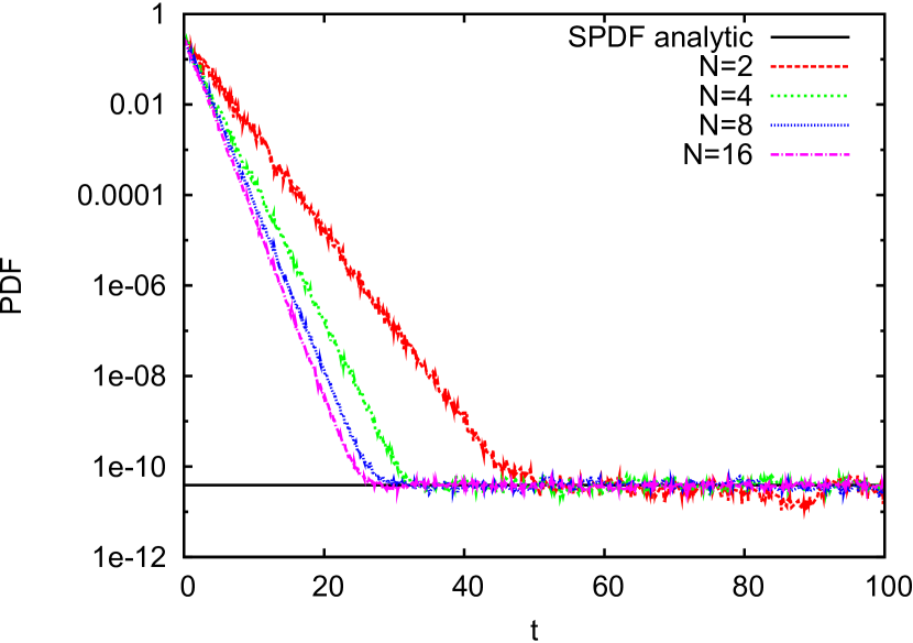
Figure 2: $PDF$ at $x=0$ obtained from $P_{i}$ by $PDF(t)=\frac{P_{i}(t)}{\Delta x}$ for the subregion containing $x=0$ for $D=0.01$ and different numbers of walkers per subregion $N$. Parameters are chosen as in run 1 (see Tab. 1).

II.1.2 Stationary probability density function

We start to calculate the SPDF $p_{st}$ in the region $[L^{-},L^{+}[$ for a small noise strength ($D=0.01$). The time step $h$ and the box size $\Delta x$ are set according to the criteria (see Tab. 1).

run	$L^{-}$	$L^{+}$	$h$	$\Delta x$	$M$
1	-1.4	1.4	0.011	0.00104869	2670
2	-1.75	1.75	0.0015	0.000387297	9037
3	-2.5	2.5	0.0001	0.00010775	46404

Table 1: Time step $h$ and box size $\Delta x$ according to convergence criteria Eq. (10) and (8), where we choose $h=\frac{h_{max}}{2}$ and $\Delta x=\frac{1}{20}L_{dif}$.

Using the results shown in Fig. 2, we set the thermalization time $T_{therm}=50$ for a run with $N=2$. Time averages after thermalization were calculated over an ensemble of $N_{T}=10^{4}$ sets P.

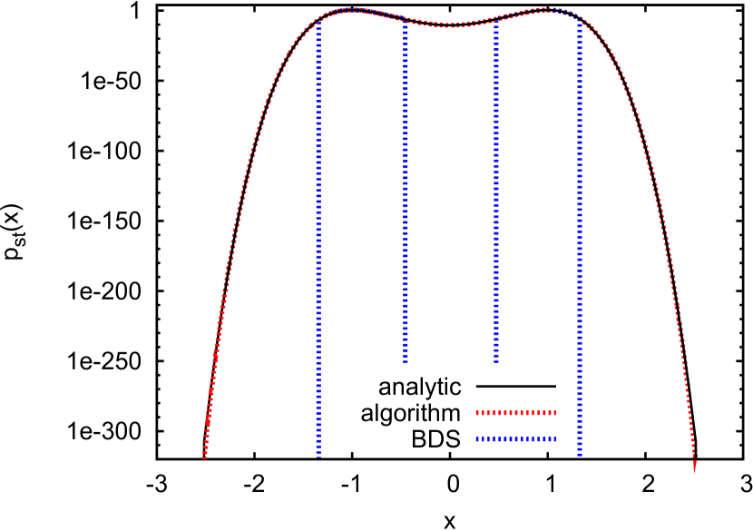
Figure 3: Estimates for the stationary probability density obtained from the algorithm for run $3$ (see Tab. 1) and by using a Brownian dynamics simulation for $D=0.01$. Analytic results are obtained from Eq. (2).

Results for the SPDF are shown in Fig. 3. The algorithm calculates the tails of the distribution down to $10^{-300}$ correctly, after a running time $T_{run}\approx 27\ hours$. We also calculate the SPDF using Brownian dynamics simulation using $N_{Brown}=10^{4}$, which stops estimating at a level of $10^{-6}$ after the same running time. Further runs were performed (see Tab. 1 (run $2$) and (run $3$)), approximating the tails down to $10^{-10}$ ($M_{group}=1136$) and $10^{-48}$ ($M_{group}=6789$) after a running time of $\approx 30\ sec$ and $\approx 10\ min$ , respectively (data not shown).

Simulations for different values of $\frac{\Delta x}{L_{dif}}$ indicate that insignificant deviations from the analytic SPDF occur for $\Delta x>\frac{1}{20}$.

II.1.3 Probability current

Next, we present that our algorithm can be used to calculate the escape rate to pass the energy barrier at $x_{max}=0$. Such problems are typical for chemical reactions Hänggi et al. (1990) and in the field of neuroscience Tuckwell (1988).

Initially, only $N$ particles are assigned at the subregion including $x_{min}=1$, so approximating an initial delta-like probability distribution for $t=0$. Furthermore, an absorbing boundary right behind the local maximum ($x_{abs}=-0.01$) is included. To fulfill normalization of the SPDF, walkers that reach $x_{abs}$ are reinjected immediately at $x_{min}$. The escape rate to pass the barrier is given by the probability current $J(x_{max})$. For small noise intensities, the probability current on top of the potential barrier can be described using Arrhenius law, namely:

$$J(x_{max})\propto e^{-\frac{\Delta U}{D}},$$ (15)

where $\Delta U=U(x_{max})-U(x_{min})=0.25$. Since strong fluctuations are rare, but possible, we will use $J(x_{abs})$ to approximate $J(x_{max})$. Probability currents $J(x_{abs})$ were recorded for each time step and averaged over a sequence of $n_{av}=\lceil\frac{0.1}{h}\rceil$ running steps, resulting in $\langle J(x_{abs})\rangle$.

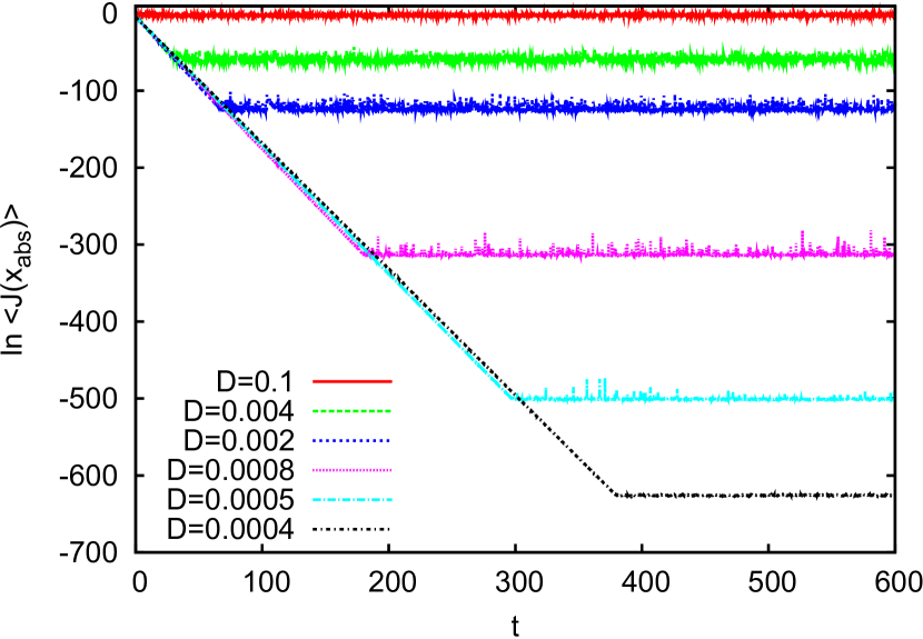
Figure 4: Time dependence of the probability current $J(x_{abs})$ obtained from our algorithm for $L^{-}=-0.02$, $L^{+}=1.39$ and decreasing noise intensities (from top to bottom). The time step is set $h=\frac{h_{max}}{2}$ and $\Delta x=\frac{1}{20}L_{dif}$. Note that $h_{max}$ and $L_{dif}$ vary according to Eq. (10) and (8), respectively, resulting in larger running times for smaller $D$.

Figure 4 shows the time dependence of $\ln\langle J(x_{abs})\rangle$. After a relaxation regime, where the current decays exponentially, the current reaches its stationary value.

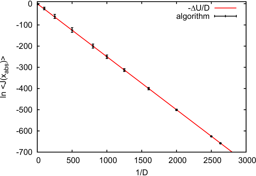
Figure 5: Stationary probability current as a function of the inverse noise strength obtained by time averaging the data partly shown in Fig. 4 in the stationary regime. Error bars show three standard deviations of the stationary data.

The values of $\ln\langle J(x_{abs})\rangle$, averaged over the stationary regime, are shown in Fig. 5 for different noise intensities. Fulfilling the criteria described above, the algorithm reproduces well Arrhenius law down to $\ln\langle J(x_{max})\rangle\approx-650$ corresponding to a current $J(x_{max})\approx 10^{-286}$.

II.1.4 Efficiency compared to weighted-ensemble Brownian dynamics simulation

In order to compare the efficiency of two algorithms, important quantities are the transient time required to first reach the steady state. Once the algorithm reaches the steady state, we quantify the size of the fluctuations by the coefficient of variation Eq. (14) at the potential’s local maximum $x=0$. The computation time mainly depends on the number of integrations $N_{int}$ needed, to reach the stationary regime.

Figure 6: Relative fluctuations plotted over the number of integration steps, needed for equilibration, for the algorithm (black) and standard (WE) simulation (red). The number of walkers per subregion is shown for each point. Simulations were done for run $1$ and $2$ (compare Tab. 1).

In order to compare the efficiency, the size of fluctuations (Eq. (14)) in the local minimum relative to $p_{st}(0)\approx 3.88717\times 10^{-11}$ during the stationary regime is plotted over $N_{int}$ in Fig. 6. The most effective algorithm would be located close to the origin. Comparing the efficiency of standard WE simulations and our algorithm, we find that WE simulations with low $N$ equilibrate faster. However, the precision highly depends on the fluctuations during the stationary regime. To produce results of same precision (same $c(0)$) both algorithms approximately need the same $N_{int}$. Usually WE simulations were performed using thousands of walkers per subregions, resulting in a low value of $c(0)$. Here runs of our algorithm producing the same $c(0)$ need much less $N$ and have memory requirements independent of $N$.

II.2 Two-dimensional systems

II.2.1 Poincaré Oscillator

As an example of a two-dimensional system with known SPDF, we consider the Poincaré oscillator Ebeling and Engel-Herbert (1980); Ebeling et al. (1986); Lekkas et al. (1988), represented by the dynamical system:

$$\begin{array}[]{cl}\dot{x}=&y\\ \dot{y}=&(\alpha-x^{2}-y^{2})y-x+\sqrt{2D}\xi(t),\\ \end{array}$$ (18)

where $\xi(t)$ represent delta correlated white Gaussian noise with zero mean. Using the energy function $H(x,y)=\frac{1}{2}(x^{2}+y^{2})$, which only depends on the distance to the origin, one can calculate the associated SPDF:

$$p_{st}(x,y)=Z^{-1}_{st}\,\exp\Large(\frac{\alpha H(x,y)-H^{2}(x,y)}{D}\Large),$$ (19)

(see appendix $\mathrm{Sec.}$ A). Since noise only applies to the $y$-direction, the lengths of a subregion $\Delta x$ and $\Delta y$ in $x$- and $y$-direction are calculated by Eq. (13) and (8), respectively. The minimum of $|f_{x}(x,y)|=|y|$ is equal to $0$, therefore, we choose $\Delta x=\Delta y\ h$, which corresponds to a first order approximation of $|f_{x}(x,y)|$ in the next subregion.

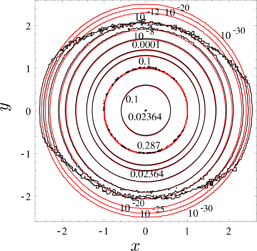
Figure 7: Contour plots of the SPDF ($D=0.1$ and $\alpha=1$) obtained from the algorithm (black), using the parameters $L_{x}^{-}=L_{y}^{-}=-3$, $L_{x}^{+}=L_{y}^{+}=3$, $T_{therm}=8$, $N_{T}=10^{3}$, $h=0.01$, $M_{x}=189737$, $M_{y}=1897$, $M_{group}=1688940$, $N=2$, ($\Delta y=\frac{1}{20}L_{dif}$) and the analytic solution (red) Eq. (19). Contour lines are labeled according to represented values of the SPDF and show the rotational symmetry. The SPDF possesses its global maximum at $H(x,y)=\frac{\alpha}{2}$, corresponding to the unit circle for our choice of $\alpha$, and a local minimum in the origin. Running time $\approx 5\ hours$.

Results for the SPDF are shown in Fig. 7. Interestingly, the algorithm approximates better the SPDF along the direction where no noise was applied. Here the SPDF is sampled down to $10^{-30}$. We found that the algorithm slightly oversamples the analytic SPDF in the tails. This is due to the statistical errors, made during the redistribution step. By reducing the size of a subregion, this error can be reduced further. Along the $y$-direction, noise is applied. Here the behavior is similar as in the one dimensional example (see above). For runs with larger $\Delta y$ (results not shown) the algorithm slightly oversamples the SPDF in the origin.

II.2.2 Bistable system with colored noise

As a further example, we calculate the SPDF of the two dimensional system:

$$\begin{array}[]{cl}\dot{x}=&x-x^{3}+y\\ \dot{y}=&-\displaystyle\frac{1}{\tau}y+\frac{1}{\tau}\sqrt{2D}\xi(t),\\ \end{array}$$ (22)

where $\tau$ denotes the time scale separation between $x$ and the colored noise $y$. The white Gaussian noise $\xi(t)$ has been already described above. This system has been studied previously in Debnath et al. (1990); Hänggi and Jung (1995). Like in the bistable system we have studied above, the SPDF has maximums at $(x,y)=(1,0)$ and $(x,y)=(-1,0)$. However, for some combinations of $\tau$ and $D$, the SPDF possesses a local minimum at $(x,y)=(0,0)$.

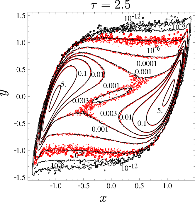
Figure 8: Contour plots of the SPDF of Eq. (22) ($D=0.1$, $\tau=2$ and $\tau=2.5$) obtained from the algorithm (black) and BDS (red) of the same running time. Parameters: (top) $L_{x}^{-}=L_{y}^{-}=-1.5$, $L_{x}^{+}=L_{y}^{+}=1.5$, $T_{therm}=10$, $N_{T}=10^{3}$, $h=0.0889$, $M_{x}=14319$, $M_{y}=1273$, $M_{group}=165003$, $N=2$,($\Delta x=\Delta y\ h$, $\Delta y=\frac{1}{20}L_{dif}$), $N_{Brown}=10^{3}$, and (bottom) $L_{x}^{-}=L_{y}^{-}=-1.5$, $L_{x}^{+}=L_{y}^{+}=1.5$, $T_{therm}=12$, $N_{T}=10^{3}$, $h=0.0889$, $M_{x}=17899$, $M_{y}=1591$, $M_{group}=206957$, $N=2$,($\Delta x=\Delta y\ h$, $\Delta y=\frac{1}{20}L_{dif}$), $N_{Brown}=10^{3}$. Running times are $19\ min$ (top) and $21\ min$ (bottom)

Plots of the SPDF are depicted in Fig. 8. Our algorithm samples the SPDF down to $10^{-12}$, whereas BDS breaks down at a level of $10^{-6}$. The minimum, occurring for $\tau=2.5$ was clearly found by the algorithm.

II.2.3 FitzHugh-Nagumo-system

As a last example, we consider the widely used FitzHugh-Nagumo-system Fitzhugh (1961), which is often used in the field of Neuroscience Lindner et al. (2004) or to study synchronization Gunton et al. (2003); Toral et al. (2003) and coherence phenomena Toral et al. (2007), represented by:

$$\begin{array}[]{cl}\dot{x}=&\frac{1}{\epsilon}(x-x^{3}-y)+\sqrt{2D_{x}}\xi_{x}(t)\\ \dot{y}=&\gamma x-y+b+\sqrt{2D_{y}}\xi_{y}(t).\\ \end{array}$$ (25)

Here $\epsilon$ denotes the timescale separation between the activator variable $x$ and the inhibitor variable $y$. $\xi_{x}(t),\xi_{y}(t)$, represent independent zero-mean delta-correlated Gaussian white noises. We want to study the stationary probability density in the case of $D_{x}=D_{y}=D$ for a time scale separation $\epsilon=0.1$. We set the parameters according to Ref. Kostur et al. (2003) to $b=1.4$, $\epsilon=0.1$ and $\gamma=2$. Thus, the system is in the excitable regime. Since the deterministic part of the equation for the activator variable increases very fast if $x$ is increased, we have to choose a time step $h=0.01$, which is small enough, that the walkers’ steps are small compared to $1$, but allows us to fulfill the criteria for the size of the subregions.

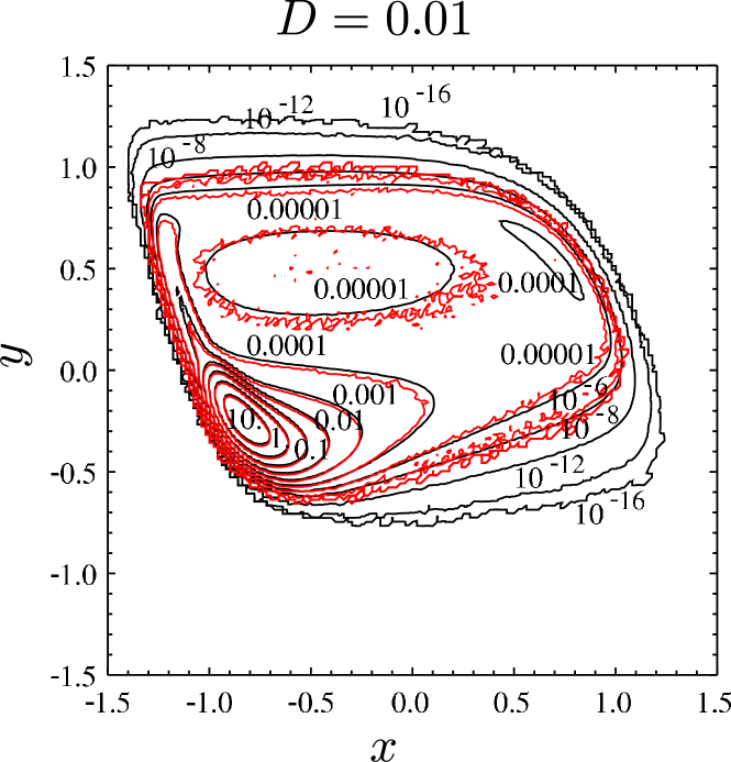
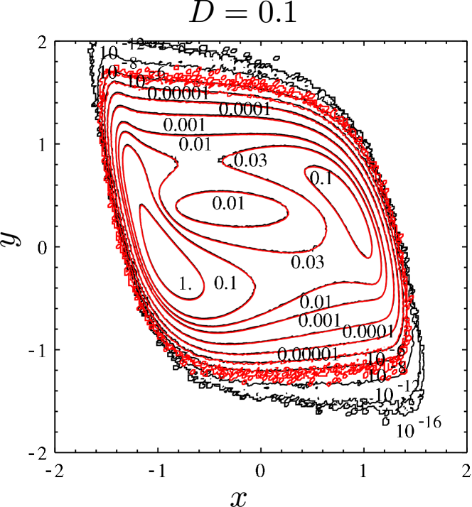
Figure 9: Contour plots of the the SPDF of Eq. (25) fod ($D=0.01$ (top) and $D=0.1$ (bottom)) obtained from the algorithm (black) and BDS (red) with the same running time. Parameters: (top) $L_{x}^{-}=L_{y}^{-}=-2$, $L_{x}^{+}=L_{y}^{+}=2$, $T_{therm}=5$, $N_{T}=10^{3}$, $h=0.01$, $M_{x}=4000$, $M_{y}=4000$, $N=2$,($\frac{\Delta x}{\sqrt{Dh}}=\frac{1}{10}$), $N_{Brown}=10^{3}$, $M_{group}=314027$, and (bottom) $L_{x}^{-}=L_{y}^{-}=-2$, $L_{x}^{+}=L_{y}^{+}=2$, $T_{therm}=3$, $N_{T}=10^{3}$, $h=0.01$, $M_{x}=1333$, $M_{y}=1333$, $N=2$, ($\Delta x=\Delta y=\frac{1}{20}L_{dif}$), $N_{Brown}=10^{3}$, $M_{group}=146568$. Running times are $27\ min$ (top) and $19\ min$ (bottom). Simulation times for the BDS were chosen three times larger.

Contour plots of the SPDF are shown in Fig. 9. Especially regions of low probability are much better sampled, using the algorithm. In the case of low diffusion ($D=0.01$, Fig. 9 (top)) the algorithm runs down to $10^{-16}$, whereas BDS stops at a level of $10^{-6}$. Especially the minimum is much better sampled by our algorithm. Note that the local maximum located in the surroundings of $(x,y)=(0.7,0.5)$ was not found by BDS. For higher diffusion values ($D=0.1$, Fig. 9 (top)), significant differences can be found only in the tails.

III Discussion

III.1 One dimensional system

In the one dimensional system (see section II.1) we succeeded to approximate the SPDF down to $10^{-300}$. If equally sized subregions are used, a huge number of subregions has to be implemented, in order to fulfill the convergence criteria (see section I.5). However, by evaluating the SPDF according to Eq. (6) the additional computational costs also reduce the fluctuations of the estimated SPDF. If the subregions are to large, the theoretical SPDF is overestimated by the algorithm in potential minimums and underestimated in the potentials maximums.

We also managed to calculate escape rates of size $10^{-286}$. Although the finite size of a subregion leads to small errors, in the calculated SPDF, Arrhenius law is well reproduced for such small probability currents.

At the stationary regime the $P_{i}$ fluctuate around their mean value, estimating the SPDF. By either increasing the number of averages $N_{T}$ or the number of walkers per subregion $N$ these fluctuations can be reduced, leading to higher precision. The estimation error scales with $\sqrt{N_{T}}$ and $\sqrt{N}$, respectively. However, increasing the number of walkers per subregion also effects the computational costs during the thermalization. Simulations for different $N$ show that runs with higher $N$ become stationary faster, but this does not compensate for the additional computational costs. We also find, that increasing $N$ slightly improves the sampling of the SPDF’s tails. Once the system is in the stationary regime the increase of the computational costs scale linearly with $N$ and $N_{T}$. An advantage of simulations with small $N$ is, that one does not need to perform running steps for subregions with $P_{i}=0$ and the number of such regions naturally increases for small $N$. We usually use the smallest possible $N=2$ and scale the estimation error by increasing $N_{T}$.

III.2 Comparison with weighted-ensemble Brownian dynamics

Since the general idea of our method was adapted from prior simulation techniques known as weighted-ensemble (WE) sampling Huber and Kim (1996); Bhatt et al. (2010); Bhatt and Bahar (2012), we want to discuss advantages and disadvantages of our algorithm in comparison with these techniques. The main difference in WE techniques is the redistribution step. Here, using WE techniques, positions and weights of all walkers are stored, and new walkers are introduced on the stored positions considering their particular weights.

In our algorithm, there is no need to store any position or weight, since walkers are randomly placed in each subregion. The resulting statistical errors can be neglected, if the size of the subregions fulfills conditions which, unfortunately, lead to much larger numbers of subregions. By averaging the probabilities, these extra computational costs contribute to an reduction of fluctuations in the stationary regime.

The comparison of the computational costs until equilibration and the achieved precision shows, that both algorithms posses the same efficiency for high precision runs.

III.3 Two dimensional systems

In the case of two dimensional systems, we found that the algorithm outperforms Brownian dynamics simulations. However, the number of subregions needed according to the criteria can be really high, especially if there are some directions without any noise. Here it is necessary to size the subregions to fulfill the criteria locally. A first step in that direction has already been done by the implementation of the grouping algorithm. We are quite confident that it is possible to reduce the computational costs by optimizing the Mesh. The analyzed examples show, that the running times highly depend on the investigated system. For the bistable system with colored noise and the FitzHugh-Nagumo-system, we obtained good results within $\approx 20$ minutes, whereas the algorithm needed about $5$ hours for the Van-der-Pol oscillator.

IV Conclusion

We provided and tested an algorithm that allows the calculation of low probabilities and low rates. The algorithm is based on WE Brownian dynamic simulations, but uses a uniform distribution of walkers within each subregion. To our findings, the resulting statistical errors can be neglected if one uses subregions small compared to the diffusion length. In contrast to WE methods, the required memory does not depend on the number of walkers, which leads to less memory requirements for runs with large numbers of walkers.

Special attention was payed to non-equilibrium dynamical systems. Applying the method to one- and two-dimensional model systems, we analyze its efficiency compared to standard Brownian dynamics simulation. Our method outperforms Brownian dynamics simulation by several orders of magnitude and its efficiency is comparable to weighted-ensemble Brownian dynamic simulations in all studied systems and lead to impressive results in regions of low probability and small rates.

Appendix A Stationary probability density of the Poincaré oscillator

Using the energy function $H(x,y)=\frac{1}{2}(x^{2}+y^{2})$, we get from $\mathrm{Eq.}$ (18) to a representation as a canonic dissipative system:

$$\begin{array}[]{cl}\dot{x}=&\partial_{y}H\\ \dot{y}=&\partial_{y}(\alpha H-H^{2})-\partial_{x}H+\sqrt{2D}\xi(t).\\ \end{array}$$ (28)

The corresponding Fokker Planck equation in the $x,y$ phase space for the SPDF $p_{st}(x,y)$ reads Ebeling and Engel-Herbert (1980):

$$\begin{array}[]{cl}\partial_{t}p_{st}=0=&-\partial_{y}H\partial_{x}p_{st}+\partial_{x}H\partial_{y}p_{st}\\ &-\partial_{y}(\partial_{y}(\alpha H-H^{2})p_{st})+D\partial_{y}^{2}p_{st}\,.\\ \end{array}$$ (31)

Using the ansatz $p_{st}(x,y)=p_{st}(H(x,y))$, the first two items at the r.h.s. cancel. The remaining second line can be integrated once. Assuming an exponentially decaying SPDF at infinitely large energies yield the disappearance of the irreversible probability flux in y-direction Graham and Haken (1971a); Haken (1975). One finds, afterwards :

$${p_{st}}\,\frac{d}{dH}(\alpha H-H^{2})\,=\,D\,\frac{d}{dH}p_{st}\,.$$ (32)

It leads to Eq. (19).

Appendix B Foundation of the algorithm

In this Appendix we show that the presented algorithm is described by a corresponding Master equation for the probability distribution density $P_{i}(t)$ for the case of a Markovian hopping process between boxes. We use a single index $i$ to label the boxes, but the argument applies to any spatial dimension $d$. We identify the dynamics of the stochastic system which shall be simulated with the discrete stochastic dynamics of the walkers. The latter is defined via the matrices of probabilities per unit time $w(i\to i^{\prime})$ which describe the hopping in the given discretized space. We assume that it shall converge for sufficiently small time scales and box lengths to the outgoing dynamics.

Let assume that we have the probability distribution density given at time $t$ in every box with index $i$. It holds

$$\sum_{i}P_{i}(t)=1.$$ (33)

We redistribute the probability in every box to $N$ walkers. In result any walker $k=1,\dots,N$ of the same box gets an identical weight

$$q_{i}^{k}(t)\,=\,{P_{i}(t)\over N}\,.$$ (34)

until the next new redistribution.

At later time $t+h$ the walkers may be still inside the box or may have jumped to other boxes. Let $U_{i}$ denote all possible box-indices which can be reached during a single step from the ${i}$-box. Then in accordance with the assumption above, the probability is $w(i\to i^{\prime})h$ that during $h$ a single walker leaves ${i}$-box and jumps to the box with index $i^{\prime}\,\in\,U_{i}$. By this hopping the walker $k$ carries the weight $q_{i}^{k}(t)$ to the new box, which step is, obviously, connected with a lost in the outgoing box. Therefore, the lost per particle for this specific hopping from $i\to i^{\prime}$ can be expressed as

$$w(i\to i^{\prime})\,h\,q_{i}^{k}(t).$$ (35)

The whole lost of weight will be realized on all possible hopping channels. It is identical for all $N$ particles being located in the present box. Hence, the full lost becomes

$$Nq_{i}^{k}(t)\sum_{i^{\prime}\in U_{i}}w(i\to i^{\prime})h=P_{i}(t)\sum_{i^{\prime}\in U_{i}}w(i\to i^{\prime})\,h\,.$$ (36)

Alternatively, one can also introduce $U^{\prime}_{i}$ as the boxes where from walkers can reach the ${i}$-box. Then, gain of weight transferred by every walker arriving at the $i$-box is expressed, if $i^{\prime}\in\,U^{\prime}_{i}$, by

$$w(i^{\prime}\to i)\,h\,q_{i^{\prime}}^{k}$$ (37)

Again, summing over the different hopping steps and considering that all the $N$ walkers inside the box with $i^{\prime}\in U^{\prime}_{i}$ reach the $i$ box, yields the gain

$$\sum_{i^{\prime}\in U^{\prime}_{i}}w(i^{\prime}\to i)hNq_{i^{\prime}}^{k}(t)=\sum_{i^{\prime}\in U^{\prime}_{i}}w(i^{\prime}\to i)hP_{i^{\prime}}(t).$$ (38)

Therefore, the balance of transported weight results in the following shift of the full weight in the $i$-box at time $t+h$ compared to the former one

$$P_{i}(t+h)\,-\,P_{i}(t)\,= \,-\,P_{i}(t)\,\sum_{i^{\prime}\in U_{i}}w(i\to i^{\prime})h$$ (39)

$$+\sum_{i^{\prime}\in U^{\prime}_{i}}w(i^{\prime}\to i)\,hP_{i^{\prime}}(t)\,,$$

plus corrections of order $O(h^{2})$ corresponding to cases in which two or more walkers jump from one box to another during the time interval $h$. After dividing by the time step $h$ and taking the limit $h\to 0$ we obtain the wanted Master equation for the discretized dynamics in the boxed phase space

$$\partial_{t}P_{i}(t)\,=\, - \,P_{i}(t)\,\sum_{i^{\prime}\in U_{i}}w(i\to i^{\prime})\,$$ (40)

$$+ \,\sum_{i^{\prime}\in U^{\prime}_{i}}w(i^{\prime}\to i)\,P_{i^{\prime}}(t)\,.$$

References

- Moss and McClintock (1989) F. Moss and P. V. McClintock, Noise in nonlinear dynamical systems, Vol. I-III (Cambridge University Press, New York, 1989).
- G. van Kampen (1992) N. G. van Kampen, Stochastic processes in physics and chemistry (North-Holland, Amsterdam, 1992).
- Nicolis and Prigogine (1977) G. Nicolis and I. Prigogine, Self-Organization in Nonequilibrium Systems: From Dissipative Structures to Order Through Fluctuations (Wiley-Interscience, New York, 1977).
- Mannella and Palleschi (1989) R. Mannella and V. Palleschi, Phys. Rev. A 40, 3381 (1989).
- Mannella (2000) R. Mannella, in Stochastic Processes in Physics, Chemistry, and Biology, Lecture Notes in Physics, Vol. 557, edited by J. A. Freund and T. Pöschel (Springer, Berlin, 2000) p. 353.
- Burrage (1999) P. Burrage, Runge-Kutta methods for stochastic differential equations, Ph.D. thesis, University of Queensland (1999).
- Kloeden and Platen (2011) P. Kloeden and E. Platen, Numerical solution of stochastic differential equations, Vol. 23 (Springer, Berlin, 2011).
- Bhanot et al. (1987) G. Bhanot, R. Salvador, S. Black, P. Carter, and R. Toral, Phys. Rev. Lett. 59, 803 (1987).
- Giardina et al. (2006) C. Giardina, J. Kurchan, and L. Peliti, Phys. Rev. Lett. 96, 120603 (2006).
- Dickson and Dinner (2010) A. Dickson and A. Dinner, Annu. Rev. Phys. Chem. 61, 441 (2010).
- Wang and P. Landau (2001) F. Wang and D. P. Landau, Phys. Rev. Lett. 86, 2050 (2001).
- Torrie and Valleau (1977) G. Torrie and J. Valleau, J. Comp. Phys. 23, 187 (1977).
- Warmflash et al. (2007) A. Warmflash, P. Bhimalapuram, and A. Dinner, J. Chem. Phys. 127, 154112 (2007).
- Allen et al. (2009) R. Allen, C. Valeriani, and P. ten Wolde, J. Phys.: Condens. Matter 21, 463102 (2009).
- Dickson et al. (2009) A. Dickson, A. Warmflash, and A. Dinner, J. Chem. Phys. 131, 154104 (2009).
- Valeriani et al. (2007) C. Valeriani, R. Allen, M. Morelli, D. Frenkel, and P. Wolde, J. Chem. Phys. 127, 114109 (2007).
- Huber and Kim (1996) G. Huber and S. Kim, Biophys. J. 70, 97 (1996).
- Bhatt et al. (2010) D. Bhatt, B. Zhang, and D. Zuckerman, J. Chem. Phys. 133, 014110 (2010).
- Zhang et al. (2010) B. Zhang, D. Jasnow, and D. Zuckerman, J. Chem. Phys. 132, 054107 (2010).
- Bhatt and Bahar (2012) D. Bhatt and I. Bahar, J. Chem. Phys. 137, 104101 (2012).
- Bhatt and Zuckerman (2011) D. Bhatt and D. Zuckerman, J. Chem. Theory Comput. 7, 2520 (2011).
- Graham and Haken (1971a) R. Graham and H. Haken, Z. Phys. 243, 289 (1971a).
- Graham and Haken (1971b) R. Graham and H. Haken, Z. Phys. 245, 141 (1971b).
- Haken (1975) H. Haken, Rev. Mod. Phys. 47, 67 (1975).
- Risken (1984) H. Risken, The Fokker Planck equation, Vol. 23 (Springer, Berlin, 1984).
- Schimansky-Geier et al. (1985) L. Schimansky-Geier, A. Tolstopjatenko, and W. Ebeling, Phys. Lett. 108A, 329 (1985).
- Ebeling and Engel-Herbert (1980) W. Ebeling and H. Engel-Herbert, Physica A 104, 378 (1980).
- Klimontovich (1980) Y. Klimontovich, Kinetic theory of elecromagnetic processes (Springer, Berlin, 1983 (in Russian: Nauka, Moscow, 1980)).
- Gilsing and Shardlow (2007) H. Gilsing and T. Shardlow, J. Comput. Appl. Math. 205, 1002 (2007).
- Gammaitoni et al. (1998) L. Gammaitoni, P. Hänggi, P. Jung, and F. Marchesoni, Rev. Mod. Phys. 70, 223 (1998).
- Hänggi et al. (1990) P. Hänggi, T. P., and N. Borkovec, Rev. Mod. Phys. 62, 251 (1990).
- Tuckwell (1988) H. Tuckwell, Introduction to theoretical neurobiology, Vol. 2 (Cambridge University Press, New York, 1988).
- Ebeling et al. (1986) W. Ebeling, H. Herzel, W. Richert, and L. Schimansky-Geier, Zeitschrift f. angew. Math. und Mech. 66, 141 (1986).
- Lekkas et al. (1988) K. Lekkas, L. Schimansky-Geier, and H. Engel-Herbert, Z. Phys. B - Condensed Matter 70, 517 (1988).
- Debnath et al. (1990) G. Debnath, F. Moss, T. Leiber, H. Risken, and F. Marchesoni, Phys. Rev. A 42, 703 (1990).
- Hänggi and Jung (1995) P. Hänggi and P. Jung, Adv. Chem. Phys. 89, 239 (1995).
- Fitzhugh (1961) R. Fitzhugh, Biophys. J. 1, 445 (1961).
- Lindner et al. (2004) B. Lindner, J. Garcıa-Ojalvo, A. Neiman, and L. Schimansky-Geier, Phys. Rept. 392, 321 (2004).
- Gunton et al. (2003) J. Gunton, R. Toral, C. Mirasso, M. Gracheva, et al., Recent. Res. Devel. Applied Phys. 6, 497 (2003).
- Toral et al. (2003) R. Toral, C. Masoller, C. Mirasso, M. Ciszak, and O. Calvo, Physica A 325, 192 (2003).
- Toral et al. (2007) R. Toral, C. Mirasso, and J. Gunton, Europhys. Lett. 61, 162 (2007).
- Kostur et al. (2003) M. Kostur, X. Sailer, and L. Schimansky-Geier, Fluct. Noise Lett. 3, 155 (2003).