Identification of fractional order systems using modulating functions method

Abstract

The modulating functions method has been used for the identification of linear and nonlinear systems. In this paper, we generalize this method to the on-line identification of fractional order systems based on the Riemann-Liouville fractional derivatives. First, a new fractional integration by parts formula involving the fractional derivative of a modulating function is given. Then, we apply this formula to a fractional order system, for which the fractional derivatives of the input and the output can be transferred into the ones of the modulating functions. By choosing a set of modulating functions, a linear system of algebraic equations is obtained. Hence, the unknown parameters of a fractional order system can be estimated by solving a linear system. Using this method, we do not need any initial values which are usually unknown and not equal to zero. Also we do not need to estimate the fractional derivatives of noisy output. Moreover, it is shown that the proposed estimators are robust against high frequency sinusoidal noises and the ones due to a class of stochastic processes. Finally, the efficiency and the stability of the proposed method is confirmed by some numerical simulations.

I Introduction

Fractional differential equations and fractional integrals are gaining importance in research community because of their capacity to accurately describe real world processes. The flow of fluid in a porous media, the conduction of heat in a semi-infinite slab, the voltage-current relation in a semi infinite transmission line are such examples of processes naturally modeled by fractional differential equations or fractional integrals.

This paper is dealing with the identification of fractional order dynamical systems. The identification of such systems has been used for instance, for the estimation of the state of charge of lead acid batteries [1], and for the identification in thermal systems [2, 3]. The goal of system identification is to estimate the parameters of a model from system input/output measurements. Different methods have been proposed for the identification of fractional order systems. Most of them consist in the generalization to fractional order systems of standard methods that were used in the identification of systems with integer order derivatives. We can classify these methods into time domain methods and frequency domain methods. Time-domain methods have been introduced for example in [4, 5], where a method based on the discretization of a fractional differential equation using Grunwald definition has been introduced, and the parameters have been estimated using least square approach. In [6], a method based on the approximation of a fractional integrator by a rational model has been proposed. In [7], the use of methods based on fractional orthogonal bases has been introduced. Other techniques can be also found for example in [8], [9], [10] and the references therein.

In this paper, we are interested in the identification of fractional order systems using modulating functions method in case of noisy measurements. Modulating functions method has been developed by Shinbrot in [11, 12] to estimate the parameters of a state space representation. Thanks to the properties of modulating functions, the fractional differential equation defining a fractional order system is transformed into a linear system of algebraic equations. Hence, instead of solving a fractional differential equation where the initial values are often unknown, the problem of identification is transformed into solving a linear system where the initial conditions are not required. Generalization of modulating functions method to fractional systems has been already proposed, for example in [13]. However, the authors of this paper proposed only to reduce the orders of the derivatives in a fractional differential equation. Moreover, the noisy case has not been considered.

In the next section, basic definitions of fractional derivatives and modulating functions are recalled. Then in Section III, modulating functions method is applied to the identification of fractional order linear systems. Error analysis in both the continuous and discrete cases are presented in Section IV. Numerical results are presented in Section V, followed by conclusions summarizing the main results obtained.

II Preliminary

In this section, first we recall the definitions and some useful properties of the Riemann-Liouville fractional derivative and modulating functions. Then, a new fractional integration by parts formula is given.

II-A Riemann-Liouville fractional derivative

Let $f$ be a continuous function defined on $\mathbb{R}$, then the Riemann-Liouville fractional derivative of $f$ is defined by (see [14] p. 62): $\forall\,t\in\mathbb{R}_{+}^{*}$,

$${\mathrm{D}}_{t}^{\alpha}f(t):=\frac{1}{\Gamma(l-\alpha)}\frac{d^{l}}{dt^{l}}\int_{0}^{t}\left(t-\tau\right)^{l-\alpha-1}f(\tau)\,d\tau,$$ (1)

where $l-1\leq\alpha<l$ with $l\in\mathbb{N}^{\ast}$, and $\Gamma(\cdot)$ is the Gamma function (see [15] p. 255). As an example, using (1) the fractional derivative of an $n^{th}$ ($n\in\mathbb{N}$) order polynomial is given by (see [14] p. 72): $\forall\,t\in\mathbb{R}_{+}^{*}$,

$${\mathrm{D}}_{t}^{\alpha}t^{n} =\frac{\Gamma(n+1)}{\Gamma(n+1-\alpha)}\,t^{n-\alpha}.$$ (2)

We assume that the fractional derivative and the Laplace transform of $f$ both exist, then the Laplace transform of the fractional derivative of $f$ is given by (see [16] p. 284): $\forall\,s\in\mathbb{C}$,

$$\mathcal{L}\left\{{\mathrm{D}}_{t}^{\alpha}f(t)\right\}(s) =s^{\alpha}\hat{f}(s)-\sum_{i=0}^{l-1}s^{i}\left[{\mathrm{D}}_{t}^{\alpha-i-1}f(t)\right]_{t=0},$$ (3)

where $\hat{f}$ denotes the Laplace transform of $f$, and $s$ denotes the variable in the frequency domain.

Finally, we recall some results on the existence and the initial values of the fractional derivative in the following proposition.

Proposition 1

(see [14] pp. 75-77) If $f\in\mathcal{C}^{l-1}([0,T])$ and $f^{(l)}\in\mathcal{L}([0,T])$ where $T\in\mathbb{R}^{*}_{+}$, then the Riemann-Liouville fractional derivative ${\mathrm{D}}_{t}^{\alpha}f(t)$ exists, where $l-1\leq\alpha<l$ with $l\in\mathbb{N}^{\ast}$. Moreover, the condition $f^{(i)}(0)=0$, for $i=0,\ldots,l-1$, is equivalent to the following condition: $\left[{\mathrm{D}}_{t}^{\alpha}f(t)\right]_{t=0}=0.$

II-B Modulating functions

Let $l\in\mathbb{N}^{*}$, $T\in\mathbb{R}^{*}_{+}$, and $g$ be a function satisfying the following properties:

$(P_{1}):$

$g\in\mathcal{C}^{l}([0,T])$;

$(P_{2}):$

$g^{(j)}(0)=g^{(j)}(T)=0,\ \forall\,j=0,1,\dots,l-1$,

then $g$ is called modulating function of order $l$ [17]. Hence, according to Proposition 1, the modulating function $g$ has also the following properties:

$(P_{3}):$

$\forall\,0\leq\beta<l$,  ${\mathrm{D}}_{t}^{\beta}g(t)$ exists;

$(P_{4}):$

$\forall\,0\leq\beta<l$,  $\left[{\mathrm{D}}_{t}^{\beta}g(t)\right]_{t=0}=0$.

II-C Fractional integration by parts

Another useful property of the modulating functions is given in the following theorem.

Theorem 1

Let $y$ be a function such that the $\alpha^{th}$ order fractional derivative exits and $g$ be a modulating function of order $l$ with $l-1\leq\alpha<l$ with $l\in\mathbb{N}^{\ast}$. Then, we have:

$$\int_{0}^{T}g(T-t)\,{\mathrm{D}}^{\alpha}_{t}y(t)\,dt=\int_{0}^{T}{\mathrm{D}}^{\alpha}_{t}g(t)\,y(T-t)\,dt,$$ (4)

where $T\in\mathbb{R}^{*}_{+}$.

Proof:

By applying the convolution theorem of the Laplace transform (see [15], p. 1020), we get:

$$\mathcal{L}\left\{\int_{0}^{T}g(T-t)\,{\mathrm{D}}^{\alpha}_{t}y(t)\,dt\right\}(s)=\hat{g}(s)\mathcal{L}\left\{{\mathrm{D}}^{\alpha}_{t}y(t)\right\}(s).$$ (5)

Then, using (3) we obtain:

$$\begin{split}&\hat{g}(s)\mathcal{L}\left\{{\mathrm{D}}^{\alpha}_{t}y(t)\right\}(s)=\\ &\qquad\hat{g}(s)s^{\alpha}\hat{y}(s)-\sum_{i=0}^{l-1}s^{i}\hat{g}(s)\left[{\mathrm{D}}_{t}^{\alpha-i-1}y(t)\right]_{t=0}.\end{split}$$ (6)

Moreover, using (3) and $(P_{4})$ we get:

$$\mathcal{L}\left\{{\mathrm{D}}^{\alpha}_{t}g(t)\right\}(s)=s^{\alpha}\,\hat{g}(s),$$ (7)

$$\mathcal{L}\left\{g^{(i)}(t)\right\}(s)=s^{i}\,\hat{g}(s),$$ (8)

for $i=0,\ldots,l-1$. Consequently, by applying (7), (8) and the inverse of the Laplace transform to (6), we obtain:

$$\begin{split}&\mathcal{L}^{-1}\left\{\hat{g}(s)\mathcal{L}\left\{{\mathrm{D}}^{\alpha}_{t}y(t)\right\}(s)\right\}(T)=\\ &\qquad\qquad\mathcal{L}^{-1}\left\{\mathcal{L}\left\{{\mathrm{D}}^{\alpha}_{t}g(t)\right\}(s)\ \hat{y}(s)\right\}(T)\\ &\qquad\qquad\qquad-\sum_{i=0}^{l-1}g^{(i)}(T)\left[{\mathrm{D}}_{t}^{\alpha-i-1}y(t)\right]_{t=0}.\end{split}$$ (9)

Using $(P_{2})$, the initial conditions $\left[{\mathrm{D}}_{t}^{\alpha-i-1}y(t)\right]_{t=0}$, for $i=0,1,\dots,l-1$, can be eliminated.

Finally, this proof can be completed by applying the convolution theorem of the Laplace transform to (9). ∎

According to the previous theorem, we can see that by working in the frequency domain: on the one hand, we can obtain an integral formula which can be considered as the generalization of the classical integration by parts formula. Another fractional integration by parts formula has also been given in [18], however the Caputo fractional derivative was involved in the formula; on the other hand, the initial conditions of the fractional derivatives of $y$ can be eliminated using a modulating function. In fact, the idea of obtaining this theorem is inspired by the recent algebraic parametric estimation technique [19, 20, 21, 22, 23, 24, 25, 26], which eliminates the unknown initial conditions by applying algebraic manipulations in the frequency domain.

III Identification of fractional order systems

III-A Fractional order linear systems

In this section, we consider a class of fractional order linear systems which are defined by the following fractional differential equation: $\forall\,t\in I=[0,T]\subset\mathbb{R}^{*}_{+}$,

$$\sum_{i=0}^{L}a_{i}\,{\mathrm{D}}^{\alpha_{i}}_{t}y(t)=\sum_{j=0}^{M}b_{j}\,{\mathrm{D}}^{\beta_{j}}_{t}u(t),$$ (10)

where $y$ is the output, $u$ is the input, $a_{i},b_{j}\in\mathbb{R}^{*}$ are unknown parameters to be identified, and $\alpha_{i},\beta_{j}\in\mathbb{R}_{+}$ are assumed $0\leq\alpha_{0}<\alpha_{1}<\cdots<\alpha_{L}$, $0\leq\beta_{0}<\beta_{1}<\cdots<\beta_{M}$ with $L,M\in\mathbb{N}$.

Let $y^{\varpi}$ be a noisy observation of $y$ on the interval $I$:

$$\forall\,t\in I,\ y^{\varpi}(t)=y(t)+\varpi(t),$$ (11)

where $\varpi$ is an integrable noise. We are going to estimate the unknown parameters in (10) using the input $u$ and the observation $y^{\varpi}$.

One of the standard methods for the identification of systems with integer order derivatives is to use the least-squares method [28]. This method was generalized to fractional order systems in [4, 5]. In this method, we need to estimate the fractional derivatives of $y$ and $u$ using a fractional order differentiator [29, 30, 31]. However, a fractional order differentiator often contains a truncated term error. An alternative method consists in solving the problem in the frequency domain by applying the Laplace transform to (10). However, according to (3), this application can produce unknown initial conditions. In the next subsection, we are going to apply modulating functions method to eliminate these unknown initial conditions.

III-B Application of modulating functions method

We denote $W=L+M+1$, $\alpha=\max\left(\alpha_{L},\beta_{M}\right)$, and $l=\lceil\alpha\rceil$, where $\lceil\alpha\rceil$ denotes the smallest integer greater than or equal to $\alpha$. Then, we take a set of modulating functions $\left\{g_{n}\right\}_{n=1}^{N}$ with $W\leq N\in\mathbb{N}$. Using Theorem 1, we can give the following proposition.

Proposition 2

Let $\left\{g_{n}\right\}_{n=1}^{N}$ be a set of modulating functions of order $l$. If we assume that $b_{0}=1$ in the fractional order linear system defined by (10), then the unknown parameters in this fractional order linear system can be estimated by solving the following linear system:

$$\left(\begin{array}[]{c}{U}_{N}\ {Y}_{N}^{\varpi}\\ \end{array}\right)\left(\begin{array}[]{c}{\tilde{B}}\\ {\tilde{A}}\\ \end{array}\right)={I}_{N},$$ (15)

where ${\tilde{B}}=\left({\tilde{b}}_{1},\cdots,{\tilde{b}}_{M}\right)^{T}$, ${\tilde{A}}=\left({\tilde{a}}_{0},\cdots,{\tilde{a}}_{L}\right)^{T}$ are estimators of the unknown parameters, and

$${U}_{N}(n,j) =-\int_{0}^{T}{\mathrm{D}}^{\beta_{j}}_{t}g_{n}(t)\,u(T-t)\,dt,$$ (16)

$${Y}_{N}^{\varpi}(n,i+1) =\int_{0}^{T}{\mathrm{D}}^{\alpha_{i}}_{t}g_{n}(t)\,y^{\varpi}(T-t)\,dt,$$ (17)

$${I}_{N}(n) =\int_{0}^{T}{\mathrm{D}}^{\beta_{0}}_{t}g_{n}(t)\,u(T-t)\,dt,$$ (18)

for $n=1,\ldots,N$, $j=1,\ldots,M$ and $i=0,\ldots,L$.

Proof:

By multiplying the modulating functions $g_{n}$ to the equation (10) and by integrating between $0$ and $T$, we get:

$$\begin{split}&\int_{0}^{T}\sum_{i=0}^{L}a_{i}\,g_{n}(T-t)\,{\mathrm{D}}^{\alpha_{i}}_{t}y(t)\,dt=\\ &\qquad\qquad\int_{0}^{T}\sum_{j=0}^{M}b_{j}\,g_{n}(T-t)\,{\mathrm{D}}^{\beta_{j}}_{t}u(t)\,dt,\end{split}$$ (19)

for $n=1,\ldots,N$. Then, using Theorem 1, we get

$$\sum_{j=1}^{M}b_{j}{U}_{N}(n,j)+\sum_{i=0}^{L}a_{i}{Y}_{N}(n,i+1)=\int_{0}^{T}{\mathrm{D}}^{\beta_{0}}_{t}g_{n}(t)u(T-t)dt,$$ (20)

where ${U}_{N}(n,j)=-\int_{0}^{T}{\mathrm{D}}^{\beta_{j}}_{t}g_{n}(t)\,u(T-t)\,dt$, and
${Y}_{N}(n,i+1)=\int_{0}^{T}{\mathrm{D}}^{\alpha_{i}}_{t}g_{n}(t)\,y(T-t)\,dt$. Finally, this proof can be completed by substituting $y$ by $y^{\varpi}$ in (20). ∎

Consequently, thanks to Theorem 1, instead of estimating (resp. calculating) the fractional derivatives of $y$ (resp. $u$), we calculate the fractional derivatives of the modulating functions. On the one hand, comparing to $y$, the modulating functions are known and without noise. On the other hand, if the fractional derivatives of $u$ cannot be analytically calculated or are difficult to calculate, we can solve the problem by calculating the ones of the modulating functions.

Finally, let us mention that since the proposed estimators are given in causal case, if we take the value of $T$ to be equal to the time where we estimate the parameters, then these estimators can be used for on-line identification applications.

IV Error analysis

In this section, we are going to study the noise effect in the integrals obtained in Proposition 2. For this purpose, we study the noise error contributions due to a high frequency sinusoidal noise and the ones due to a class of stochastic processes in continuous case and in discrete case, respectively.

IV-A Error analysis in continuous case

There are many applications where the output signal is corrupted by a sinusoidal noise of higher frequency [26]. Hence, we assume that the noise $\varpi$ is a high frequency sinusoidal noise in this subsection.

By writing $y^{\varpi}=y+\varpi$, the integral ${Y}_{N}^{\varpi}(n,i+1)$ given in (17), for $n=1,\ldots,N$ and $i=0,\ldots,L$, can be divided into:

$${Y}_{N}^{\varpi}(n,i+1)={Y}_{N}(n,i+1)+e_{N}^{\varpi}(n,i+1),$$ (21)

where ${Y}_{N}(n,i+1)$ is given in (20), and the associated noise error contribution is given by:

$$e_{N}^{\varpi}(n,i+1)=\int_{0}^{T}{\mathrm{D}}^{\alpha_{i}}_{t}g_{n}(t)\,\varpi(T-t)\,dt.$$ (22)

Consequently, the estimation errors for the estimators given in Proposition 2 only come from these noise error contributions. In the following proposition, we give error bounds for these noise error contributions.

Proposition 3

We assume that $\forall\,t\in I$, $\varpi(t)=c\sin(\omega t+\phi)$ with $c,\omega\in\mathbb{R}^{*}_{+}$ and $\phi\in[0,2\pi[$. Moreover, we assume that ${\mathrm{D}}^{\alpha_{i}+1}_{t}g_{n}(t)$ exists and is continuous on $[0,T]$, for $n=1,\ldots,N$ and $i=0,\ldots,L$. Then, we have:

$$\left|e_{N}^{\varpi}(n,i+1)\right|\leq\frac{c}{\omega}TC_{\alpha_{i}+1}+\frac{c}{\omega}\left|\left[{\mathrm{D}}_{t}^{\alpha_{i}}g_{n}(t)\right]_{t=T}\right|,$$ (23)

where $C_{\alpha_{i}+1}=\displaystyle\sup_{t\in[0,T]}\left|{\mathrm{D}}^{\alpha_{i}+1}_{t}g_{n}(t)\right|$, and $e_{N}^{\varpi}(n,i+1)$ is given by (22).

Proof:

Since $\frac{d}{dt}\left\{{\mathrm{D}}^{\alpha_{i}}_{t}g_{n}(t)\right\}={\mathrm{D}}^{\alpha_{i}+1}_{t}g_{n}(t)$ exists, then by applying integration by parts and $(P_{4})$, we get:

$$\begin{split}e_{N}^{\varpi}(n,i+1)=&\int_{0}^{T}{\mathrm{D}}^{\alpha_{i}}_{t}g_{n}(t)\,c\sin(\omega(T-t)+\phi)\,dt\\ =&-\frac{c}{\omega}\int_{0}^{T}{\mathrm{D}}^{\alpha_{i}+1}_{t}g_{n}(t)\,\cos(\omega(T-t)+\phi)\,dt\\ &\quad+\frac{c}{\omega}\cos(\phi)\left[{\mathrm{D}}_{t}^{\alpha_{i}}g_{n}(t)\right]_{t=T}.\end{split}$$ (24)

If ${\mathrm{D}}^{\alpha_{i}+1}_{t}g_{n}(t)\in\mathcal{C}([0,T])$, then this proof can be completed using (24). ∎

According to the previous proposition, if the frequency of the sinusoidal noise is high, then the associated noise error contributions can be negligible. Consequently, the estimators given in Proposition 2 can cope with this kind of noises.

IV-B Error analysis in discrete case

From now on, we assume that the noisy observation $y^{\varpi}$ defined in (11) is given in a discrete case. Let $y^{\varpi}(t_{j})=y(t_{j})+\varpi(t_{j})$ be a noisy discrete observation of $y$ given with an equidistant sampling period $T_{s}$, where $T_{s}=\frac{T}{m}$, $m\in\mathbb{N}^{*}$, and $t_{j}=jT_{s}$, for $j=0,\cdots,m$.

Since $y^{\varpi}$ is a discrete measurement, we apply a numerical integration method to approximate the integrals in (15). Let $w_{0}\geq 0$, $w_{m}\geq 0$ and $w_{j}>0$ for $j=1,\dots,m-1$ be the weights for a given numerical integration method, where weight $a_{0}$ (resp. $a_{m}$) is set to zero when there is an infinite value at $t_{0}=0$ (resp. $t_{m}=T$). Then, the integral ${Y}_{N}^{\varpi}(n,i+1)$ given in (17), for $n=1,\ldots,N$ and $i=0,\ldots,L$, can be approximated by:

$${Y}_{N,m}^{\varpi}(n,i+1):=T_{s}\sum_{j=0}^{m}{w_{j}}\,g_{n}^{(\alpha_{i})}(t_{j})\,y^{\varpi}(t_{m-j}),$$ (25)

where $g_{n}^{(\alpha_{i})}(t_{j}):=\left[{\mathrm{D}}^{\alpha_{i}}_{t}g_{n}(t)\right]_{t=t_{j}}$. The integrals given in (16) and (18) can be approximated in a similar way.

By writing $y^{\varpi}(t_{j})=y(t_{j})+\varpi(t_{j})$, we get:

$${Y}_{N,m}^{\varpi}(n,i+1)={Y}_{N,m}(n,i+1)+e_{N,m}^{\varpi}(n,i+1),$$ (26)

where

$${Y}_{N,m}(n,i+1) =T_{s}\displaystyle\sum_{j=0}^{m}{w_{j}}\,g_{n}^{(\alpha_{i})}(t_{j})\,y(t_{m-j}),$$ (27)

$$e_{N,m}^{\varpi}(n,i+1) =T_{s}\displaystyle\sum_{j=0}^{m}{w_{j}}\,g_{n}^{(\alpha_{i})}(t_{j})\,\varpi(t_{m-j}).$$ (28)

Thus the integral ${Y}_{N}^{\varpi}(n,i+1)$ is corrupted by two sources of errors:

• the numerical error which comes from a numerical integration method,

• the noise error contribution $e_{N,m}^{\varpi}(n,i+1)$.

Consequently, the estimation errors for the estimators given in Proposition 2 come from both the numerical errors and the noise error contributions in the discrete noisy case.

It is well known that if the value of $T$ is set, then when $T_{s}$ tends to $0$, $i.e.$ $m\rightarrow+\infty$, the numerical errors tend to $0$. In the next subsection, we are going to study the effect of the sampling period on the noise error contributions.

IV-C Influence of sampling period on noise error contributions

In this subsection, we consider a family of noises which are stochastic processes satisfying the following conditions:

$(C_{1}):$

for any $t,s\in I$, $t\neq s$, $\varpi(t)$ and $\varpi(s)$ are independent;

$(C_{2}):$

the mean value function of $\varpi(\cdot)$ denoted by $\mathrm{E}[\cdot]$ belongs to $\mathcal{L}(I)$;

$(C_{3}):$

the variance function of $\varpi(\cdot)$ denoted by $\mathrm{Var}[\cdot]$ is bounded on $I$.

Note that the white Gaussian noise and the Poisson noise satisfy these conditions. Then, we can give the following proposition.

Proposition 4

Let $\varpi(\cdot)$ be a stochastic process satisfying conditions $(C_{1})-(C_{3})$, and $\varpi(t_{j})$, for $j=0,\cdots,m$, be a sequence of $\{\varpi(\cdot)\}$ with an equidistant sampling period $T_{s}$. If ${\mathrm{D}}^{\alpha_{i}}_{t}g_{n}(t)\in\mathcal{L}^{2}(I)$, then we have the following convergence in mean square of the noise error contribution in the integral ${Y}_{N}^{\varpi}(n,i+1)$ given in (17), for $n=1,\ldots,N$ and $i=0,\ldots,L$:

$$e_{N,m}^{\varpi}(n,i+1)\xLongrightarrow[T_{s}\rightarrow 0]{\mathcal{L}^{2}(I)}\int_{0}^{T}{\mathrm{D}}^{\alpha_{i}}_{t}g_{n}(t)\,\mathrm{E}\left[\varpi(T-t)\right]\,dt,$$ (29)

where $e_{N,m}^{\varpi}(n,i+1)$ is given in (28). Moreover, if $\forall\,t\in I$, $\mathrm{E}\left[\varpi(t)\right]=0$, then we have:

$$e_{N,m}^{\varpi}(n,i+1)\xLongrightarrow[T_{s}\rightarrow 0]{\mathcal{L}^{2}(I)}0.$$ (30)

The proof of the previous proposition can be obtained in a similar way to the one given in [27]. Moreover, a similar result was studied using the non-standard analysis in [32].

Consequently, according to the previous proposition, the noise error contributions can be increasing with respect to the sampling period.

Finally, let us mention that solving the linear system given in Proposition 2 in noisy case is related to the matrix perturbation theory. The accuracy and the stability of the proposed estimators not only depend on the noise error contributions, but also depend on the condition number of the associated matrix. This condition number depends both on the input and the output of the fractional order system and on the used modulating functions. In general, we should choose the modulating functions that can give a small condition number. This study is out of the scope of this paper.

V Simulation results

In order to illustrate the accuracy and robustness with respect to corrupting noises of the proposed estimators, we present some numerical results in this section.

Let us consider a fractional order system defined by the following fractional differential equation: $\forall\,t\in[0,8]$,

$$a_{0}{\mathrm{D}}^{\alpha_{0}}_{t}y(t)+a_{1}{\mathrm{D}}^{\alpha_{1}}_{t}y(t)+a_{2}{\mathrm{D}}^{\alpha_{2}}_{t}y(t)=u(t),$$ (31)

where $a_{0}=3$, $a_{1}=2$, $a_{2}=1$, $\alpha_{0}=0$, $\alpha_{1}=0.5$ and $\alpha_{2}=1.5$. We assume that the output is $y(t)=\sin(3t)+1$. Hence, the initial conditions of $y$ are not equal to $0$. Moreover, the expression of the input can be obtained using (2) and the following formula (see [33] p. 83):

$$\begin{split}&{\mathrm{D}}_{t}^{\alpha_{i}}\sin(3t)=\\ &\frac{3t^{1-\alpha_{i}}}{\Gamma(2-\alpha_{i})}\,{}_{1}{\mathrm{F}}_{2}\left(1;\frac{1}{2}(2-\alpha_{i}),\frac{1}{2}(3-\alpha_{i});-\frac{1}{4}3^{2}t^{2}\right),\end{split}$$ (32)

where ${}_{p}{\mathrm{F}}_{q}\left(c_{1},\ldots,c_{p};d_{1},\ldots,d_{q};\cdot\right)$ is the generalized hypergeometric function given in [33] p. 303.

In our identification procedure, we use the following modulating functions, the fractional derivative of which are simple to calculate:

$$g_{n}(t)=(T-t)^{6+n}t^{6+N+1-n},$$ (33)

where $n=1,2,\cdots,N$ with $N=13$. The value of $T$ is taken to be equal to the time where we estimate the parameters. Let us recall that this kind of functions has been obtained when the algebraic parametric estimation technique was applied to the parameter estimation for signals described by differential equations [21].

In the two following examples, we estimate the parameters $a_{0}$, $a_{1}$ and $a_{2}$ using the noisy observation of $y$ where the noise is a high frequency sinusoidal noise and a gaussian noise, respectively. Moreover, we apply the trapezoidal rule to numerically approximate the integrals in our estimators.

Example 1. In this example, we assume that $y^{\varpi}(t_{j})=y(t_{j})+0.5\sin(10^{3}t_{j})$ with $T_{s}=0.01$. We can see this discrete noisy signal in Figure 1. In our identification procedure, we take $T=t_{i}$ for $t_{i}\in[1.8,8]$. The obtained estimations and the associated relative estimation errors are shown in Figure 2 and Figure 3. Hence, we can see that the proposed estimators can cope with a high frequency sinusoidal noise.

Example 2. In this example, we assume that $y^{\varpi}(t_{j})=y(t_{j})+\sigma\varpi(t_{j})$, where $T_{s}=0.01$, $\varpi(t_{j})$ is simulated from a zero-mean white Gaussian $iid$ sequence, and $\sigma\in\mathbb{R}_{+}^{*}$ is adjusted in such a way that the signal-to-noise ratio is equal to $SNR=22\text{dB}$. This noisy observation is shown in Figure 4. The obtained estimations and the associated relative estimation errors are given in Figure 5 and Figure 6. We can see that the proposed estimators are robust against a gaussian noise.

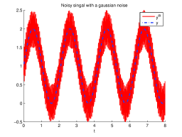
Figure 1: The noise-free output and its noisy observation.

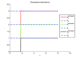
Figure 2: The exact parameters and their estimations with a sinusoidal noise.

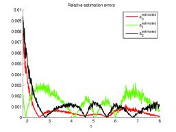
Figure 3: Relative estimation errors in the sinusoidal noise case.

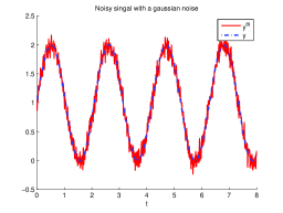
Figure 4: The noise-free output and its noisy observation.

VI Conclusions

In this paper, the modulating functions method has been generalized to the on-line identification problem of fractional order systems. Using this method, the unknown parameters have been estimated by solving a linear system of algebraic equations involving the input and the noisy output. Thanks to the properties of modulating functions, we do not need to estimate the fractional derivatives of the output, to calculate the ones of the input. We do not need to know the initial conditions either. Moreover, the integral given in the estimators can reduce the noise effects due to a high frequency sinusoidal noise or a class of stochastic processes. The efficiency and the robustness against corrupting noises have been confirmed by numerical examples. In order to improve the robustness against noises, some methods such as the instrumental variable method will be applied [34]. It was mentioned that the proposed estimators also depend on the choice of modulating functions. This problem will be studied in the future work. Moreover, the estimation of the fractional derivative orders in a time-delayed fractional order system will be considered.

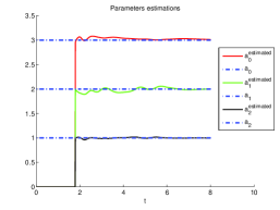
Figure 5: The exact parameters and their estimations with a gaussian noise.

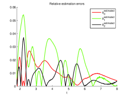
Figure 6: Relative estimation errors in the gaussian noise case.

References

- [1] J. Sabatier, M. Aoun, A. Oustaloup, G. Gregoire, F. Ragot and P. Roy, Fractional system identification for lead acid battery state of charge estimation, Signal Processing, 86, pp. 2645-2657, 2006.
- [2] J.D. Gabano and T. Poinot, Fractional modeling and identification of thermal systems, Signal Processing, 91, pp. 531-541, 2011.
- [3] J.D. Gabano, T. Poinot and H. Kanoun, Identification of a thermal system using continuous linear parameter-varying fractional modelling, IET Control Theory & Applications, 5, 7, pp. 889-899, 2011.
- [4] A. Oustaloup, L. Le Lay and B. Mathieu, Identification of non integer order system in the time domain, in proceeding IEEE CESA’96, SMC IMACS Multiconference, Computational Engineering in Systems Application, Symposium on Control, Optimisation and Supervision, Lille, France, July 9-12, 1996.
- [5] A. Djouambia, A. Vodab and A. Charefc, Recursive prediction error identification of fractional order models, Communications in Nonlinear Science and Numerical Simulation, 17, 6, pp. 2517-2524, 2012.
- [6] J.C. Trigeassou, T. Poinot, J. Lin, A. Oustaloup and F. Levron, Modeling and identification of a non integer order system, in: Proceedings of the ECC99,European Control Conference, Karlsruhe, Germany, 1999.
- [7] M. Aoun, R. Malti, F. Levron and A. Oustaloup, Synthesis of fractional Laguerre basis for system approximation, Automatica, 43, 9, pp. 1640-1648, 2007.
- [8] O. Cois, A. Oustaloup, T. Poinot and J.L. Battaglia, Fractional state variable filter for system identification by fractional model, in: IEEE 6th European Control Conference ECC2001. Porto, Portugal, 2001.
- [9] O. Cois, A. Oustaloup, E. Battaglia and J.L. Battaglia, Non integer model from modal decomposition for time domain system identification, In: proceedings of 12th IFAC Symposium on System Identification, SYSID, Santa Barbara, USA, 2000.
- [10] R. Malti, M. Aoun, J. Sabatier and A. Oustaloup, Tutorial on system identification using fractional differentiation models, in: 14th FAC Symposium on System Identification, Newcastle, Australia, 2006.
- [11] M. Shinbrot, On the analysis of linear and nonlinear dynamic systems from transient-response data, National Advisory Committee for Aeronautics NACA, Technical Note 3288, Washington, 1954.
- [12] M. Shinbrot, On the analysis of linear and nonlinear systems. Trans. ASME, pp. 547-552, 1957.
- [13] T. Janiczek, Generalization of modulating functions method in the fractional differential equations, Bulletin of the academy of Sciences, 58, 4, pp. 593-599, 2010.
- [14] I. Podlubny, Fractional Differential Equations, vol. 198 of Mathematics in Science and Engineering, Academic Press, New York, NY, USA, 1999.
- [15] M. Abramowitz and I.A. Stegun, editeurs. Handbook of mathematical functions. GPO, 1965.
- [16] A.A. Kilbas, H.M. Srivastava, and J.J. Trujillo, Theory and Applications of Fractional Differential Equations, vol. 204 of North-Holland Mathematics Studies, Elsevier, Amsterdam, The Netherlands, 2006.
- [17] H.A. Preising, D.W.T. Rippin, Theory and application of the modulating function method. I: Review and theory of the method and theory of the splinetype modulating functions, Computers and Chemical Engineering, 17, pp. 1-16, 1993.
- [18] I. Podlubny and Y.Q. Chen, Adjoint fractional differential expressions and operators. In: Proceedings of the ASME 2007 International Design Engineering Technical Conferences & Computers and Information in Engineering Conference IDETC/CIE 2007, Las Vegas, NV, September 4-7, 2007.
- [19] M. Fliess and H. Sira-Ramírez, An algebraic framework for linear identification, ESAIM Control Optim. Calc. Variat., 9, 2003, pp. 151-168.
- [20] M. Fliess and H. Sira-Ramírez, Closed-loop parametric identification for continuous-time linear systems via new algebraic techniques, in H. Garnier, L. Wang (Eds): Identification of Continuous-time Models from Sampled Data, pp. 363-391, Springer-Verlag, London, 2008.
- [21] M. Mboup, Parameter estimation for signals described by differential equations, Applicable Analysis, 88, pp. 29-52, 2009.
- [22] D.Y. Liu, O. Gibaru and W. Perruquetti, Parameters estimation of a noisy sinusoidal signal with time-varying amplitude. In: 19th Mediterranean conference on Control and automation (MED’11), Corfu, Greece, 2011.
- [23] D.Y. Liu, O. Gibaru, W. Perruquetti, M. Fliess and M. Mboup, An error analysis in the algebraic estimation of a noisy sinusoidal signal. In: 16th Mediterranean conference on Control and automation (MED’08), Ajaccio, France, 2008.
- [24] R. Ushirobira, W. Perruquetti, M. Mboup and M. Fliess, Algebraic parameter estimation of a biased sinusoidal waveform signal from noisy data, 16th IFAC Symposium on System Identification, Brussels, Belgium, 2012.
- [25] W. Perruquetti, P. Fraisse, M. Mboup and R. Ushirobira, An algebraic approach for Humane posture estimation in the sagital plane using accelerometer noisy signal, 51st IEEE Conference on Decision and Control, Hawaii, USA, 2012.
- [26] J.R. Trapero, H. Sira-Ramírez and V.F. Battle, An algebraic frequency estimator for a biased and noisy sinusoidal signal, Signal Processing, 87, pp. 1188-1201, 2007.
- [27] D.Y. Liu, O. Gibaru and W. Perruquetti, Error analysis of Jacobi derivative estimators for noisy signals. Numerical Algorithms, 58, 1, pp. 53-83, 2011.
- [28] L. Ljung, System Identification: Theory for the User, Prentice Hall PTR Upper Saddle River, NJ, USA, 1999.
- [29] D.L. Chen, Y.Q. Chen and D.Y. Xue, Digital Fractional Order Savitzky-Golay Differentiator, IEEE Transactions on Circuits and Systems II: Express Briefs, 58, 11, pp. 758-762, 2011.
- [30] D.Y. Liu, O. Gibaru, W. Perruquetti and T.M. Laleg-Kirati, Fractional order differentiation by integration with Jacobi polynomials, 51st IEEE Conference on Decision and Control, Hawaii, USA, 2012.
- [31] D.Y. Liu, O. Gibaru and W. Perruquetti, Non-asymptotic fractional order differentiators via an algebraic parametric method, 1st International Conference on Systems and Computer Science, Villeneuve d’ascq, France, 2012.
- [32] M. Fliess, Analyse non standard du bruit, C.R. Acad. Sci. Paris Ser. I, 342, pp. 797-802, 2006.
- [33] K.S. Miller and B. Ross, An Introduction to the Fractional Calculus and Fractional Differential Equations, Wiley, New York, 1993.
- [34] H. Garnier and L. Wang (Eds.), Identification of continuous-time models from sampled data, Springer-Verlag, London, 2008.