Joint Maximum Sum-Rate Receiver Design and Power Adjustment for Multihop Wireless Sensor Networks

Abstract

In this paper, we consider a multihop wireless sensor network (WSN) with multiple relay nodes for each hop where the amplify-and-forward (AF) scheme is employed. We present a strategy to jointly design the linear receiver and the power allocation parameters via an alternating optimization approach that maximizes the sum rate of the WSN. We derive constrained maximum sum-rate (MSR) expressions along with an algorithm to compute the linear receiver and the power allocation parameters with the optimal complex amplification coefficients for each relay node. Computer simulations show good performance of our proposed methods in terms of sum rate compared to the method with equal power allocation.

Index Terms—  Maximum sum-rate (MSR), power allocation, multihop, wireless sensor networks (WSNs)

1 Introduction

Recently, there has been a growing research interest in wireless sensor networks (WSNs) as their unique features allow a wide range of applications in the areas of defence, environment, health and home [1]. They are usually composed of a large number of densely deployed sensing devices which can transmit their data to the desired user through multihop relays [2]. Low complexity and high energy efficiency are the most important design characteristics of communication protocols [3] and physical layer techniques employed for WSNs. The performance and capacity of WSNs can be significantly enhanced through exploitation of spatial diversity with cooperation between the nodes [2]. In a cooperative WSN, nodes relay signals to each other in order to propagate redundant copies of the same signals to the destination nodes. Among the existing relaying schemes, the amplify-and-forward (AF) and the decode-and-forward (DF) are the most popular approaches [4].

Due to limitations in sensor node power, computational capacity and memory [1], some power allocation methods have been proposed for WSNs to obtain the best possible SNR or best possible quality of service (QoS) [5] at the destinations. The majority of the previous literature considers a source and destination pair, with one or more randomly placed relay nodes. These relay nodes are usually placed with uniform distribution [6], equal distance [7], or in line [8] with the source and destination. The reason of these simple considerations is that they can simplify complex problems and obtain closed-form solutions. A single relay AF system using mean channel gain channel state information (CSI) is analyzed in [9], where the outage probability is the criterion used for optimization. For DF systems, a near-optimal power allocation strategy called the Fixed-Sum-Power with Equal-Ratio (FSP-ER) scheme based on partial CSI has been developed in [6]. This near-optimal scheme allocates one half of the total power to the source node and splits the remaining half equally among selected relay nodes. A node is selected for relay if its mean channel gain to the destination is above a threshold. Simulations show that this scheme significantly outperforms existing power allocation schemes. One is the ’Constant-Power scheme’ where all nodes serve as relay nodes and all nodes including the source node and relay nodes transmit with the same power. The other is the ’Best-Select scheme’ where only the node with the largest mean channel gain to the destination is chosen as the relay node.

In this paper, we consider a general multihop wireless sensor networks where the AF relaying scheme is employed. Our strategy is to jointly design the linear maximum sum-rate (MSR) receiver (w) and the power allocation parameter (a) that contains the optimal complex amplification coefficients for each relay node via an alternating optimization approach. It can be considered as a constrained optimization problem where the objective function is the sum-rate (SR) and the constraint is a bound on the power levels among the relay nodes. Then the constrained MSR solutions for the linear receiver and the power allocation parameter can be derived. The proposed strategy and algorithm are not only applicable to simple 2-hop WSNs but also to general multihop WSNs with multi relay nodes and destination nodes. Another novelty is that we make use of the Generalized Rayleigh Quotient [13] to solve the optimization problem in an alternating fashion.

This paper is organized as follows. Section 2 describes the multihop WSN system model. Section 3 develops the joint MSR receiver design and power allocation strategy. Section 4 presents the proposed alternating optimization algorithm to maximize the sum rate. Section 5 presents and discusses the simulation results, while Section 6 provides some concluding remarks.

2 System Model

Consider a general m-hop wireless sensor network (WSN) with multiple parallel relay nodes for each hop, as shown in Fig. 1. The WSN consists of $N_{0}$ source nodes, $N_{m}$ destination nodes and $N_{r}$ relay nodes which are separated into $m-1$ groups: $N_{1}$,$N_{2}$, … ,$N_{m-1}$. We will focus on a time division scheme with perfect synchronization, for which all signals are transmitted and received in separate time slots. The sources first broadcast the $N_{0}\times 1$ signal vector s to the first group of relay nodes. We consider an amplify-and-forward (AF) cooperation protocol. Each group of relay nodes receives the signal, amplifies and rebroadcasts them to the next group of relay nodes (or the destination nodes). In practice, we need to consider the constraints on the transmission policy. For example, each transmitting node would transmit during only one phase. In our WSN system, we assume that each group of relay nodes transmits the signal to the nearest group of relay nodes (or destination nodes) directly.

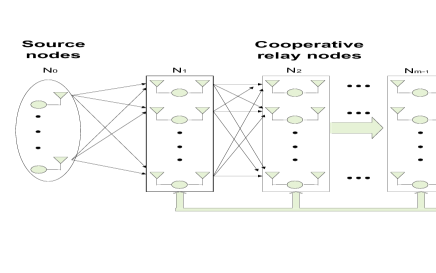
Fig. 1: $m$-hop WSN with $N_{0}$ sources, $N_{m}$ destinations and $N_{r}$ relays.

Let $\textbf{H}_{s}$ denote the $N_{1}\times{N_{0}}$ channel matrix between the source nodes and the first group of relay nodes, $\textbf{H}_{d}$ denote the $N_{m}\times{N_{m-1}}$ channel matrix between the $(m-1)$th group of relay nodes and destination nodes, and $\textbf{H}_{i-1,i}$ denote the $N_{i}\times{N_{i-1}}$ channel matrix between two groups of relay nodes as described by

$$\textbf{H}_{s}=\begin{bmatrix}\textbf{h}_{s,1}\\ \textbf{h}_{s,2}\\ \vdots\\ \textbf{h}_{s,N_{1}}\\ \end{bmatrix},~{}~{}~{}\textbf{H}_{d}=\begin{bmatrix}\textbf{h}_{m-1,1}\\ \textbf{h}_{m-1,2}\\ \vdots\\ \textbf{h}_{m-1,N_{m}}\\ \end{bmatrix},~{}~{}~{}\textbf{H}_{i-1,i}=\begin{bmatrix}\textbf{h}_{i-1,1}\\ \textbf{h}_{i-1,2}\\ \vdots\\ \textbf{h}_{i-1,N_{i}}\\ \end{bmatrix},~{}~{}~{}$$ (1)

where $\textbf{h}_{s,j}=[h_{s,j,1},h_{s,j,2},...,h_{s,j,N_{0}}]$ for $j=1,2,...,N_{1}$ is a row vector between source nodes and the $j$th relay of the first group of relay nodes, $\textbf{h}_{m-1,j}=[h_{m-1,j,1},h_{m-1,j,2},...,h_{m-1,j,N_{m-1}}]$ for $j=1,2,...,N_{m}$ is a row vector between the $(m-1)$th group of relay nodes and the $j$th destination node and $\textbf{h}_{i-1,j}=[h_{i-1,j,1},h_{i-1,j,2},...,h_{i-1,j,N_{i-1}}]$ for $j=1,2,...,N_{i}$ is a row vector between the $(i-1)$th group of relay nodes and the $j$th relay of the $i$th group of relay nodes. The received signal at the $i$th group of relay nodes ($\textbf{x}_{i}$) for each phase can be expressed as:

Phase 1:

$$\textbf{x}_{1}=\textbf{H}_{s}\textbf{s}+\textbf{v}_{1},$$ (2)

$$\textbf{y}_{1}=\textbf{F}_{1}\textbf{x}_{1},$$ (3)

Phase 2:

$$\textbf{x}_{2}=\textbf{H}_{1,2}\textbf{A}_{1}\textbf{y}_{1}+\textbf{v}_{2},$$ (4)

$$\textbf{y}_{2}=\textbf{F}_{2}\textbf{x}_{2},$$ (5)

⋮

Phase $i$: ($i=2,3,...,m-1$)

$$\textbf{x}_{i}=\textbf{H}_{i-1,i}\textbf{A}_{i-1}\textbf{y}_{i-1}+\textbf{v}_{i},$$ (6)

$$\textbf{y}_{i}=\textbf{F}_{i}\textbf{x}_{i},$$ (7)

At the destination nodes, the received signal can be expressed as

$$\textbf{d}=\textbf{H}_{d}\textbf{A}_{m-1}\textbf{y}_{m-1}+\textbf{v}_{d},$$ (8)

where v is a zero-mean circularly symmetric complex additive white Gaussian noise (AWGN) vector with covariance matrix $\sigma^{2}\textbf{I}$. $\textbf{A}_{i}={\rm diag}\{a_{i,1},a_{i,2},...,a_{i,N_{i}}\}$ is a diagonal matrix whose elements represent the amplification coefficient of each relay of the $i$th group. $\textbf{F}_{i}$ denotes the normalization matrix which can normalize the power of the received signal for each relay of the $i$th group of relays.(see the appendix to find the expression of $\textbf{F}_{i}$.) Please note that the property of the matrix vector multiplication $\textbf{Ay}=\textbf{Ya}$ will be used in the next section, where Y is the diagonal matrix form of the vector y and a is the vector form of the diagonal matrix A. At the receiver, a linear MMSE detector is considered where the optimal filter and optimal amplification coefficients are calculated. The optimal amplification coefficients are transmitted to the relays through the feedback channel. And the block marked with a Q[$\cdot$] represents a decision device.

3 Proposed Joint Maximum Sum-Rate Design of the Receiver and the Power Allocation

By substituting (2)-(7) into (8), we can get

$$\begin{split}\textbf{d}=&\textbf{C}_{0,m-1}\textbf{s}+\textbf{C}_{1,m-1}\textbf{v}_{1}+\textbf{C}_{2,m-1}\textbf{v}_{2}\\ &+...+\textbf{C}_{m-1,m-1}\textbf{v}_{m-1}+\textbf{v}_{d}\\ =&\textbf{C}_{0,m-1}s+\sum_{i=1}^{m-1}\textbf{C}_{i,m-1}\textbf{v}_{i}+\textbf{v}_{d}\end{split}$$ (9)

where

$$\textbf{C}_{i,j}=\left\{\begin{array}[]{ll}\prod_{k=i}^{j}\textbf{B}_{k},&\textrm{if $i\leqslant j$,}\\ \textbf{I},&\textrm{if $i>j$}.\\ \end{array}\right.$$ (10)

and

$$\textbf{B}_{0}=\textbf{H}_{s}$$ (11)

$$\textbf{B}_{i}=\textbf{H}_{i,i+1}\textbf{A}_{i}\textbf{F}_{i}~{}~{}~{}~{}~{}\textrm{for}~{}i=1,~{}2,~{}...,~{}m-2$$ (12)

$$\textbf{B}_{m-1}=\textbf{H}_{d}\textbf{A}_{m-1}\textbf{y}_{m-1}$$ (13)

We focus on the system which consists of one source node. Therefore, the expression of the Sum Rate (SR) for our m-hop WSNs is expressed as

$${\rm SR}=\frac{1}{m}\log_{2}\left[1+\frac{\sigma_{s}^{2}}{\sigma_{n}^{2}}\frac{\textbf{w}^{H}\textbf{C}_{0,m-1}\textbf{C}_{0,m-1}^{H}\textbf{w}}{\textbf{w}^{H}(\sum_{i=1}^{m}\textbf{C}_{i,m-1}\textbf{C}_{i,m-1}^{H})\textbf{w}}\right]$$ (14)

where w is the linear receiver, and $(\cdot)^{H}$ denotes the complex-conjugate (Hermitian) transpose. Let

$$\boldsymbol{\phi}=\textbf{C}_{0,m-1}\textbf{C}_{0,m-1}^{H}$$ (15)

and

$$\textbf{Z}=\sum_{i=1}^{m}\textbf{C}_{i,m-1}\textbf{C}_{i,m-1}^{H}$$ (16)

The expression for the sum-rate can be written as

$${\rm SR}=\frac{1}{m}\log_{2}\left(1+\frac{\sigma_{s}^{2}}{\sigma_{n}^{2}}\frac{\textbf{w}^{H}\boldsymbol{\phi}\textbf{w}}{\textbf{w}^{H}\textbf{Z}\textbf{w}}\right)=\frac{1}{m}\log_{2}(1+ax)$$ (17)

where

$$a=\frac{\sigma_{s}^{2}}{\sigma_{n}^{2}}$$ (18)

and

$$x=\frac{\textbf{w}^{H}\boldsymbol{\phi}\textbf{w}}{\textbf{w}^{H}\textbf{Z}\textbf{w}}$$ (19)

Since $\frac{1}{m}\log_{2}(1+ax)$ is a monotonically increasing function of $x$ ($a>0$), the problem of maximizing the sum rate is equivalent to maximizing $x$. In this section, we consider the case where the total power of the relay nodes in each group is limited to some value $P_{T,i}$ (local constraint). The proposed method can be considered as the following optimization problem:

$$\begin{split}&[\textbf{w}_{opt},\textbf{a}_{1,opt},...,\textbf{a}_{m-1,opt}]~{}=\arg\max_{\textbf{w},\textbf{a}_{1},...,\textbf{a}_{m-1}}\frac{\textbf{w}^{H}\boldsymbol{\phi}\textbf{w}}{\textbf{w}^{H}\textbf{Z}\textbf{w}},\\ &{~{}~{}~{}~{}~{}~{}~{}~{}~{}\textrm{subject to}}~{}P_{i}=P_{T,i},~{}i=1,2,...,m-1.\end{split}$$ (20)

where $P_{i}$ as defined above is the transmitted power of the $i$th group of relays, and $P_{i}=N_{i+1}\textbf{a}_{i}^{H}\textbf{a}_{i}$. We can notice that the expression $\frac{\textbf{w}^{H}\boldsymbol{\phi}\textbf{w}}{\textbf{w}^{H}\textbf{Z}\textbf{w}}$ in (20) is the Generalized Rayleigh Quotient, therefore the optimal solution of our maximization problem can be solved: $\textbf{w}_{opt}$ is any eigenvector corresponding to the dominant eigenvalue of $\textbf{Z}^{-1}\boldsymbol{\phi}$.

In order to obtain the optimal power allocation vector $\textbf{a}_{opt}$, we rewrite $\frac{\textbf{w}^{H}\boldsymbol{\phi}\textbf{w}}{\textbf{w}^{H}\textbf{Z}\textbf{w}}$ and the expression is given by

$$\frac{\textbf{w}^{H}{\boldsymbol{\phi}}\textbf{w}}{\textbf{w}^{H}\textbf{Z}\textbf{w}}=\frac{\textbf{a}_{i}^{H}\textbf{M}_{i}\textbf{a}_{i}}{\textbf{a}_{i}^{H}{\rm diag}\{\textbf{w}_{i}^{H}\textbf{P}_{i}\textbf{w}_{i}\}\textbf{a}_{i}+\textbf{w}_{i}^{H}\textbf{T}_{i}\textbf{w}_{i}},~{}{\rm for}~{}i=1,~{}2,...,~{}m-1,$$ (21)

where
$\textbf{M}_{i}={\rm diag}\{\textbf{w}_{i}^{H}\textbf{C}_{i+1,m-1}\textbf{H}_{i,i+1}\textbf{F}_{i}\}\textbf{C}_{0,i-1}\textbf{C}_{0,i-1}^{H}\times$
${\rm diag}\{\textbf{F}_{i}^{H}\textbf{H}_{i,i+1}^{H}\textbf{C}_{i+1,m-1}^{H}\textbf{w}_{i}\}$,

$\textbf{P}_{i}=\textbf{C}_{i+1,m-1}\textbf{H}_{i,i+1}\textbf{F}_{i}\}(\sum_{k=1}^{i}\textbf{C}_{k,i-1}\textbf{C}_{k,i-1}^{H})\times$
${\rm diag}\{\textbf{F}_{i}^{H}\textbf{H}_{i,i+1}^{H}\textbf{C}_{i+1,m-1}^{H}\}$
and
$\textbf{T}_{i}=(\sum_{k=i+1}^{m}\textbf{C}_{k,m-1}\textbf{C}_{k,m-1}^{H})$.

Since the multiplication of any constant value and a eigenvector is still the eigenvector of the matrix, we can express the receive filter as

$$\textbf{w}_{i}=\frac{\textbf{w}_{opt}}{\sqrt{\textbf{w}_{opt}^{H}(\sum_{k=i+1}^{m}\textbf{C}_{k,m-1}\textbf{C}_{k,m-1}^{H})\textbf{w}_{opt}}}$$ (22)

Therefore, we can obtain

$$\textbf{w}_{i}^{H}(\sum_{k=i+1}^{m}\textbf{C}_{k,m-1}\textbf{C}_{k,m-1}^{H})\textbf{w}_{i}=1=\frac{N_{i+1}\textbf{a}_{i}^{H}\textbf{a}_{i}}{P_{T,i}}$$ (23)

By substituting (23) into (21) and using $\textbf{M}_{i}$ and $\textbf{N}_{i}$ given above to simplify the expression of (21), we obtain

$$\frac{\textbf{w}^{H}\boldsymbol{\phi}\textbf{w}}{\textbf{w}^{H}\textbf{Z}\textbf{w}}=\frac{\textbf{a}_{i}^{H}\textbf{M}_{i}\textbf{a}_{i}}{\textbf{a}_{i}^{H}\textbf{N}_{i}\textbf{a}_{i}}~{}~{}~{}~{}{\rm for}~{}i=1,~{}2,...,~{}m-1$$ (24)

We can notice that the expression $\frac{\textbf{a}^{H}\textbf{M}_{i}\textbf{a}}{\textbf{a}_{i}^{H}\textbf{N}_{i}\textbf{a}_{i}}$ in (26) is the Generalized Rayleigh Quotient, therefore the optimal solution of our maximization problem can be solved: $\textbf{a}_{i,opt}$ is any eigenvector corresponding to the dominant eigenvalue of $\textbf{N}_{i}^{-1}\textbf{M}_{i}$, and satisfying $\textbf{a}_{i,opt}^{H}\textbf{a}_{i,opt}=\frac{P_{T,i}}{N_{i+1}}$. The solutions of $\textbf{w}_{opt}$ and $\textbf{a}_{i,opt}$ depend on each other. Therefore it is necessary to iterate them with an initial value of $\textbf{a}_{i}$ ($i=1,2,...,m-1$) to obtain the optimum solutions.

4 Proposed Alternating Maximization Algorithm

In this section, we devise our proposed alternating maximization algorithm which computes the linear receive filter and the power allocation parameters that maximize the sum rate of the WSN. In particular, we employ two methods to calculate the dominant eigenvectors. The first one is the QR algorithm [18] which calculates all the eigenvalues and eigenvectors of a matrix. We can choose the dominant eigenvector among them. The second one is the power method [18] which only calculates the dominant eigenvector of a matrix. Therefore, the computational complexity can be reduced. Table 1 shows a summary of our proposed algorithm which will be used for the simulations.

Table 1: Summary of the Proposed Algorithm

Initialize the algorithm by setting
${\textbf{A}_{i}}=\sqrt{\frac{P_{T,i}}{N_{i}N_{i+1}}}\textbf{I}$   for $i=1,2,...,m-1$
For each iteration:
1. Compute $\boldsymbol{\phi}$ and Z in (15) and (16).
2. Using QR algorithm or power method to compute the
dominate eigenvector of $\textbf{Z}^{-1}\boldsymbol{\phi}$, denoted as $\textbf{w}_{opt}$.
3. For $i=1,2,...,m-1$
a) Compute $\textbf{M}_{i}$ and $\textbf{N}_{i}$ in (24) and (25).
b) Using the QR algorithm or power method to compute the
dominate eigenvector of $\textbf{N}_{i}^{-1}\textbf{M}_{i}$, denoted as $\textbf{a}_{i}$.
c) To ensure the local power constraint $\textbf{a}_{i,opt}^{H}\textbf{a}_{i,opt}=\frac{P_{T,i}}{N_{i+1}}$,
compute $\textbf{a}_{i,opt}=\sqrt{\frac{P_{T,i}}{N_{i+1}\textbf{a}_{i}^{H}\textbf{a}_{i}}}\textbf{a}_{i}$.

Tong, we should include a short paragraph here discussing the required complexity and the convergence issues.

5 Simulations

In this section, we numerically study the sum-rate performance of our proposed joint MSR design of the receiver and power allocation methods and compare them with the equal power allocation method [6] which allocates the same power level equally for all links from the relay nodes. We consider a 3-hop ($m$=3) wireless sensor network. The number of source nodes ($N_{0}$), two groups of relay nodes ($N_{1},N_{2}$) and destination nodes ($N_{3}$) are 1, 4, 4, 2 respectively. We consider an AF cooperation protocol. The quasi-static fading channel (block fading channel) is considered in our simulations whose elements are Rayleigh random variables (with zero mean and unit variance) and assumed to be invariant during the transmission of each packet. In our simulations, the channel is assumed to be known at the destination nodes. For channel estimation algorithms for WSNs and other low-complexity parameter estimation algorithms, one can refer to [15] and [16]. During each phase, the sources transmit the QPSK modulated packets with 1500 symbols. The noise at the destination nodes is modeled as circularly symmetric complex Gaussian random variables with zero mean. When perfect (error free) feedback channel between destination nodes and relay nodes is assumed to transmit the amplification coefficients, it can be seen from Fig. 3 that our proposed method can achieve better sum-rate performance than the equal power allocation method. When using the power method to calculate the dominant eigenvector, it can get a very similar result to the QR algorithm. In practice, the feedback channel can not be error free. In order to study the impact of feedback channel errors on the performance, we employ the binary symmetric channel (BSC) as the model for the feedback channel and quantize each complex amplification coefficient to an 8-bit binary value (4 bits for the real part, 4 bits for the imaginary part). Vector quantization methods [17] can also be employed for increased spectral efficiency. The error probability (Pe) of BSC is fixed at $10^{-3}$. The dashed curves in Fig. 3 show the performance degradation compared with the performance when using a perfect feedback channel. To show the performance tendency of the BSC for other values of Pe, we fix the SNR at 10 dB and choose Pe ranging form 0 to $10^{-2}$. The performance curves are shown in Fig. 4, which illustrates the sum-rate performance versus Pe of our two proposed methods. It can be seen that along with the increase in Pe, their performance becomes worse.

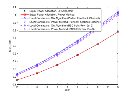
Fig. 2: Sum-rate performance versus SNR of our proposed joint maximum sum-rate design of the receiver and power allocation strategy for a 3-hop WSN, compared with equal power allocation method.

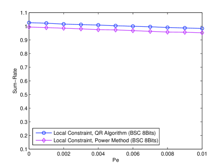
Fig. 3: Sum-rate performance versus Pe of our proposed joint strategy when employing BSC as the model for the feedback channel.

6 Conclusions

A joint MSR receiver design and power allocation strategy has been proposed for general multihop WSNs. It has been shown that our proposed strategy achieves a significantly better performance than the equal power allocation method. Possible extensions to this work may include the study of the complexity and the requirement for the feedback channel.

7 appendix

Here, we derive the expression of $\textbf{F}_{i}$ which is denoted in Section 2.

$$\textbf{F}_{i}={\rm diag}\{E(|x_{i,1}|^{2}),E(|x_{i,2}|^{2}),...,E(|x_{i,N_{i}}|^{2})\}^{-\frac{1}{2}}$$ (25)

where

$$E(|x_{i,j}|^{2}=\left\{\begin{array}[]{ll}\sigma_{s}^{2}|\textbf{h}_{s,j}|^{2}+\sigma_{n}^{2},~{}~{}~{}~{}~{}~{}~{}~{}~{}~{}~{}~{}~{}~{}~{}~{}~{}~{}~{}~{}~{}~{}~{}~{}~{}~{}~{}~{}~{}~{}~{}~{}~{}~{}~{}~{}~{}~{}\textrm{for $i=1$,}\\ \textbf{h}_{i-1,j}\textbf{A}_{i-1}E(\textbf{y}_{i-1}\textbf{y}_{i-1}^{H})\textbf{A}_{i-1}^{H}\textbf{h}_{i-1,j}^{H}+\sigma_{n}^{2},\\ ~{}~{}~{}~{}~{}~{}~{}~{}~{}~{}~{}~{}~{}~{}~{}~{}~{}~{}~{}~{}~{}~{}~{}~{}~{}~{}~{}~{}~{}~{}~{}~{}~{}~{}~{}~{}~{}~{}~{}~{}~{}~{}~{}~{}~{}~{}~{}~{}~{}~{}\textrm{for $i=2,3,...,m$}.\\ \end{array}\right.$$ (26)

$$E(\textbf{y}_{i}\textbf{y}_{i}^{H})=\left\{\begin{array}[]{ll}\textbf{F}_{i}(\sigma_{s}^{2}\textbf{H}_{s}\textbf{H}_{s}^{H}+\sigma_{n}^{2}\textbf{I})\textbf{F}_{i}^{H},~{}~{}~{}~{}~{}~{}~{}~{}~{}~{}~{}~{}~{}~{}~{}~{}~{}~{}~{}~{}~{}~{}~{}~{}~{}\textrm{for $i=1$,}\\ \textbf{F}_{i}[\textbf{H}_{i-1,i}\textbf{A}_{i-1}E(\textbf{y}_{i-1}\textbf{y}_{i-1}^{H})\textbf{A}_{i-1}^{H}\textbf{H}_{i-1,i}^{H}+\sigma_{n}^{2}\textbf{I}]\textbf{F}_{i}^{H}\\ ~{}~{}~{}~{}~{}~{}~{}~{}~{}~{}~{}~{}~{}~{}~{}~{}~{}~{}~{}~{}~{}~{}~{}~{}~{}~{}~{}~{}~{}~{}~{}~{}~{}~{}~{}~{}~{}~{}~{}~{}~{}~{}~{}~{}~{}~{}~{}~{}~{}~{}~{}~{}\textrm{for $i=2,3,...,m$}.\\ \end{array}\right.$$ (27)

References

- [1] I. F. Akyildiz, W. Su, Y. Sankarasubramaniam, and E. Cayirci, ”A Survey on Sensor Networks,” IEEE Commun. Mag., vol. 40, pp. 102-114, Aug. 2002.
- [2] J. N. Laneman, D. N. C. Tse and G. W. Wornell, ”Cooperative diversity in wireless networks: Efficient protocols and outage behavior,” IEEE Trans. Inf. Theory, vol. 50, no. 12, pp. 3062-3080, Dec. 2004.
- [3] H. Li and P. D. Mitchell, ”Reservation packet medium access control for wireless sensor networks,” in Proc. IEEE PIMRC, Sep. 2008.
- [4] Y. W. Hong, W. J. Huang, F. H. chiu, and C. C. J. Kuo, ”Cooperative Communications in Resource-Constrained Wireless Networks,” IEEE Signal Process. Mag., vol. 24, pp. 47-57, May 2007.
- [5] T. Q. S. Quek, H. Shin. and M. Z. win, ”Robust Wireless Relay Networks: Slow Power Allocation With Guaranteed QoS,” IEEE J. Sel. Topics Signal Process., vol. 1, no. 4, pp. 700-713, Dec. 2007.
- [6] J. Luo, R. S. Blum, L. J. Cimini, L. J. Greenstein, and A. M. Haimovich ”Decode-Forward Cooperative Diversity with Power Allocation in Wireless Networks” IEEE Trans. Wireless Commun., vol. 6, no. 3, pp. 793-799, Mar. 2007.
- [7] W. Su, A. K. Sadek, and K. J. R. Liu, ”Ser performance analysis and optimum power allocation for decode and forward cooperation protocol in wireless networks,” in Proc. IEEE WCNC, pp. 984-989, Mar. 2005.
- [8] D. Gunduz and E. Erkip, ”Opportunistic cooperation by dynamic resource allocation,” IEEE Trans. Wireless Commun., vol. 6, pp. 1446-1454, Apr. 2007.
- [9] X. Deng and A. Haimovich, ”Power allocation for cooperative relaying in wireless networks,” IEEE Trans. Commun., vol. 50, no. 12, pp. 3062-3080, Jul. 2005.
- [10] P. Clarke and R. C. de Lamare, ”Joint Transmit Diversity Optimization and Relay Selection for Multi-Relay Cooperative MIMO Systems Using Discrete Stochastic Algorithms,” IEEE Communications Letters, vol.15, no.10, pp.1035-1037, October 2011.
- [11] P. Clarke and R. C. de Lamare, ”Transmit Diversity and Relay Selection Algorithms for Multirelay Cooperative MIMO Systems” IEEE Transactions on Vehicular Technology, vol.61, no. 3, pp. 1084-1098, October 2011.
- [12] R. C. de Lamare, “Joint iterative power allocation and linear interference suppression algorithms for cooperative DS-CDMA networks”, IET Communications, vol. 6, no. 13 , 2012, pp. 1930-1942.
- [13] R. D. Juday, ”Generalized Rayleigh quotient approach to filter optimization” J. Opt. Soc., vol. 15, no. 4, pp. 777-790, Apr. 1998.
- [14] S. Haykin, Adaptive Filter Theory, 4th ed. Englewood Cliffs, NJ: Prentice-Hall, 2002.
- [15] T. Wang, R. C. de Lamare, and P. D. Mitchell, ”Low-Complexity Set-Membership Channel Estimation for Cooperative Wireless Sensor Networks,” IEEE Trans. Veh. Technol., vol. 60, no. 6, May, 2011.
- [16] R. C. de Lamare and P. S. R. Diniz, ”Set-Membership Adaptive Algorithms based on Time-Varying Error Bounds for CDMA Interference Suppression,” IEEE Trans. Veh. Technol., vol. 58, no. 2, Feb. 2009.
- [17] R. C. de Lamare and A. Alcaim, ”Strategies to improve the performance of very low bit rate speech coders and application to a 1.2 kb/s codec,” IEE Proceedings- Vision, image and signal processing. vol. 152, no. 1, Feb. 2005.
- [18] D. S. Watkins, Fundamentals of Matrix Computations, 2nd ed. John Wiley & Sons, New York, 2002.
- [19] R. C. de Lamare and R. Sampaio-Neto, ”Minimum Mean Squared Error Iterative Successive Parallel Arbitrated Decision Feedback Detectors for DS-CDMA Systems,” IEEE Transactions on Communications. vol. 56, no. 5, May, 2008.
- [20]