Cubic-scaling algorithm and self-consistent field for the random-phase approximation with second-order screened exchange

Abstract

The random-phase approximation with second-order screened exchange (RPA+SOSEX) is a model of electron correlation energy with two caveats: its accuracy depends on an arbitrary choice of mean field, and it scales as $\mathcal{O}(n^{5})$ operations and $\mathcal{O}(n^{3})$ memory for $n$ electrons. We derive a new algorithm that reduces its scaling to $\mathcal{O}(n^{3})$ operations and $\mathcal{O}(n^{2})$ memory using controlled approximations and a new self-consistent field that approximates Brueckner coupled-cluster doubles (BCCD) theory with RPA+SOSEX, referred to as Brueckner RPA (BRPA) theory. The algorithm comparably reduces the scaling of second-order Møller-Plesset (MP2) perturbation theory with smaller cost prefactors than RPA+SOSEX. Within a semiempirical model, we study H₂ dissociation to test accuracy and H_n rings to verify scaling.

I Introduction

Density functional theory (DFT) and coupled-cluster (CC) theory are the two dominant paradigms for the computation of many-electron ground states with complementary capabilities. Both theories are built upon the independent-orbital and self-consistent field (SCF) structure of Hartree-Fock (HF) theory QCtextbook . DFT proves the existence of an exact density functional HohenbergKohn for which there are approximations KohnSham ; LDA enabling routine simulation of thousands of electrons bigDFT that scale as $\mathcal{O}(n^{3})$ operations and $\mathcal{O}(n^{2})$ memory for $n$ electrons. CC theory is a systematically improvable hierarchy of methods CCreview indexed by $p\geq 2$ that scale as $\mathcal{O}(n^{2p+2})$ operations and $\mathcal{O}(n^{2p})$ memory. In practice, DFT is limited by accuracy and CC theory is limited by cost.

The random phase approximation (RPA) is a natural point of convergence in the ongoing development of CC theory and DFT. RPA emerges from truncated versions of CC methods as reduced-complexity methods that retain a significant fraction of the CC correlation energy RPAfromCC . RPA also occurs when DFT is used to approximate the polarization function in the adiabatic-connection fluctuation-dissipation formula for the correlation energy RPAfromACFD . This formula might become a part of more accurate density functionals, but it has a higher cost and complexity oldfastRPA than conventional density functionals. In both cases, a balance of cost and accuracy is being sought with RPA.

The electron correlation energy model that we consider in this paper is the RPA correlation energy plus the second-order screened exchange (SOSEX) energy VASP_SOSEX . RPA+SOSEX is exact for one electron and to second order in perturbation theory. It agrees with quantum Monte Carlo benchmarks of the uniform electron gas QMC_egas to within 0.002 Ha/electron Freeman_SOSEX . Benchmarks on inhomogeneous systems show mean absolute errors of 0.002 Ha/atom for cohesive energies of solids in a 5-solid test set VASP_SOSEX , 0.008 Ha/molecule for atomization energies of molecules in the G2-1 test set bench_SOSEX , and 0.010 Ha/atom for correlation energies of first and second row atoms bench_SOSEX . These atomic and molecular RPA+SOSEX results approach but fail to surpass the accuracy of second-order Møller-Plesset (MP2) perturbation theory RPA3rd ; SOSEX_implementation and the B3LYP density functional SE_SOSEX . Also, any RPA+SOSEX energy depends on a mean field choice and is not unique VASP_SOSEX .

The goal of this paper is to further develop RPA+SOSEX as a compromise between the cost of DFT and the accuracy of CC theory. Known algorithms for RPA+SOSEX VASP_SOSEX and similar models SOSEX_implementation require $\mathcal{O}(n^{5})$ operations and either $\mathcal{O}(n^{3})$ or $\mathcal{O}(n^{4})$ memory. By utilizing an auxiliary basis set auxiliary , fast interaction kernel summation fast_kernel_sum , and a low-rank approximation of energy denominators Laplace , we design a new algorithm to reduce the cost to $\mathcal{O}(n^{3})$ operations and $\mathcal{O}(n^{2})$ memory. We define a precise RPA+SOSEX total energy with a unique choice of mean field based on Brueckner orbitals Brueckner_orbitals that is designed to approximate Brueckner coupled-cluster doubles (BCCD) theory BCCD . This is referred to as Brueckner RPA (BRPA) theory.

It is important to be pragmatic about the short-term value of BRPA theory and a fast RPA+SOSEX algorithm. Despite its construction, BRPA is not a good approximation of BCCD. The approximations used to retain the RPA+SOSEX form are too crude. For a given basis, a fast RPA+SOSEX calculation will have a large cost relative to conventional DFT. With the continued reduction of average errors in density functionals DFTaccuracy and a correlation of DFT and RPA error outliers DFTerrors , it is unclear whether the cost is warranted without additional research.

The paper proceeds as follows. BRPA theory is derived in Sec. II as a truncation of BCCD theory. The SCF structure of BRPA theory is emphasized. The three main components of a fast RPA+SOSEX algorithm are introduced in Sec. III. This includes a nonstandard choice of primary and auxiliary basis, which simplifies the cost accounting and algorithm design. In Sec. IV, the tensor structure in existing RPA algorithms oldfastRPA ; SOSEX_implementation is reviewed and extended to RPA+SOSEX. The novel structure of RPA+SOSEX theory enables a significant reduction in the number of its variables. Fast and conventional RPA+SOSEX algorithms are designed in Sec. V as pseudocode. A detailed leading-order cost analysis is given instead of a crude scaling analysis. We study applications to a semiempirical H_n model in Sec. VI. The accuracy of BRPA theory is tested on H₂, and the scaling of RPA+SOSEX algorithms is confirmed with H_n calculations for large $n$. The implications for future work are discussed in Sec. VII. This includes implementation in established electronic structure codes, basis set convergence problems, and further development of correlation models. We conclude in Sec. VIII with a brief consideration of RPA as a distinct electronic structure paradigm.

II Brueckner RPA (BRPA) theory

The common origin of all post-HF methods is the many-electron Hamiltonian in second quantization notation QCtextbook ,

$$\hat{H}=E_{0}+h_{q}^{p}\hat{c}_{p}^{\dagger}\hat{c}_{q}+\tfrac{1}{4}\widetilde{V}_{rs}^{pq}\hat{c}_{p}^{\dagger}\hat{c}_{q}^{\dagger}\hat{c}_{s}\hat{c}_{r},$$ (1)

where $\hat{c}_{p}$ are the fermion lowering operators of spin-orbitals. Spin-orbital indices are labeled by $\{p,q,r,s\}$. Any tensor or product of tensors with repeated indices has an implicit sum over those indices unless they appear unrepeated in a tensor or product of tensors or in an explicit sum in the same equation. This notation is related to the standard bracket notation QCtextbook as

$$h_{q}^{p} =\langle p|h|q\rangle=\int d\mathbf{x}d\mathbf{y}\phi_{p}^{*}(\mathbf{x})h(\mathbf{x},\mathbf{y})\phi_{q}(\mathbf{y}),$$

$$V_{rs}^{pq} =\langle pq|rs\rangle=\int d\mathbf{x}d\mathbf{y}\phi_{p}^{*}(\mathbf{x})\phi_{q}^{*}(\mathbf{y})V(\mathbf{x},\mathbf{y})\phi_{r}(\mathbf{x})\phi_{s}(\mathbf{y}),$$

$$\widetilde{V}_{rs}^{pq} =\langle pq||rs\rangle=\langle pq|rs\rangle-\langle pq|sr\rangle,$$ (2)

where $\mathbf{x}$ and $\mathbf{y}$ are spin-space coordinates, $h(\mathbf{x},\mathbf{y})$ is the single-electron Hamiltonian, $V(\mathbf{x},\mathbf{y})$ is the inter-electron interaction, $\phi_{p}(\mathbf{x})$ are the spin-orbital wavefunctions, and $\widetilde{X}_{rs}^{pq}=X_{rs}^{pq}-X_{sr}^{pq}$ is a tensor antisymmetrization operation. The operators have symmetries $h(\mathbf{x},\mathbf{y})=h(\mathbf{y},\mathbf{x})^{*}$ and $V(\mathbf{x},\mathbf{y})=V(\mathbf{y},\mathbf{x})$.

We define a reference Slater determinant, $|\Phi\rangle$, by splitting the set of orbitals into virtual orbitals labeled by $\{a,b,c,d\}$ and $n$ occupied orbitals labeled by $\{i,j,k,l\}$. $|\Phi\rangle$ is defined by

$$\hat{c}_{i}^{\dagger}|\Phi\rangle=0,\ \ \ \hat{c}_{a}|\Phi\rangle=0,\ \ \ \langle\Phi|\Phi\rangle=1,$$ (3)

uniquely up to a global phase. When combined with fermion anticommutation, $\hat{c}_{p}^{\dagger}\hat{c}_{q}=\delta_{q}^{p}-\hat{c}_{q}\hat{c}_{p}^{\dagger}$ and $\hat{c}_{p}\hat{c}_{q}=-\hat{c}_{q}\hat{c}_{p}$, Eq. (3) is sufficient to calculate all expectation values of $|\Phi\rangle$.

HF theory posits the minimization of $E_{\mathrm{HF}}=\langle\Phi|\hat{H}|\Phi\rangle$ and diagonalization of particle and hole subspaces, $\langle\Phi|\hat{c}_{a}\hat{H}\hat{c}_{b}^{\dagger}|\Phi\rangle$ and $\langle\Phi|\hat{c}_{i}^{\dagger}\hat{H}\hat{c}_{j}|\Phi\rangle$. For local minima in $E_{\mathrm{HF}}$, this is equivalent to diagonalization of a Fock matrix,

$$f_{q}^{p0}=h_{q}^{p}+\widetilde{V}_{iq}^{ip}=\epsilon_{p}\delta_{q}^{p},$$ (4)

or equivalently a Fock operator in spin-space,

$$f^{0}(\mathbf{x},\mathbf{y}) =h(\mathbf{x},\mathbf{y})+v(\mathbf{x})\delta(\mathbf{x}-\mathbf{y})-\rho(\mathbf{x},\mathbf{y})V(\mathbf{x},\mathbf{y}),$$

$$\rho(\mathbf{x},\mathbf{y}) =\phi_{i}(\mathbf{x})\phi_{i}^{*}(\mathbf{y}),\ \ \ v(\mathbf{x})=\int d\mathbf{y}V(\mathbf{x},\mathbf{y})\rho(\mathbf{y},\mathbf{y}),$$

$$\ \ \ \ \int d\mathbf{y}f^{0}(\mathbf{x},\mathbf{y})\phi_{p}(\mathbf{y})=\epsilon_{p}\phi_{p}(\mathbf{x}),$$ (5)

with the canonical SCF structure between $\phi_{p}(\mathbf{x})$ and $f^{0}(\mathbf{x},\mathbf{y})$. The total energy consistent with the Fock matrix is

$$E_{\mathrm{HF}} =E_{0}+h_{i}^{i}+\tfrac{1}{2}\widetilde{V}_{ij}^{ij}$$ (6a)

$$=E_{0}+\tfrac{1}{2}(h_{i}^{i}+f_{i}^{i0}).$$ (6b)

The orbital energies are approximate excitation energies,

$$\epsilon_{a} =\langle\Phi|\hat{c}_{a}\hat{H}\hat{c}_{a}^{\dagger}|\Phi\rangle-E_{\mathrm{HF}},$$

$$\epsilon_{i} =E_{\mathrm{HF}}-\langle\Phi|\hat{c}_{i}^{\dagger}\hat{H}\hat{c}_{i}|\Phi\rangle,$$ (7)

which is known as Koopmans’ theorem Koopmans .

II.1 Brueckner coupled-cluster doubles (BCCD) theory

The basic structure of CC theory is to solve $\hat{H}|\Psi\rangle=E|\Psi\rangle$ approximately as a projected eigenvalue problem CCreview . It defines a cluster operator, $\hat{T}$, from the linear span of a set of operators, $\mathcal{S}$, omitting identity, $\hat{I}$, which only alters the normalization,

$$\langle\Phi|\hat{X}^{\dagger} \exp(-\hat{T})\hat{H}|\Psi\rangle=E\langle\Phi|\hat{X}^{\dagger}\exp(-\hat{T})|\Psi\rangle,\ \ \ \hat{X}\in\mathcal{S},$$

$$|\Psi\rangle =\exp(\hat{T})|\Phi\rangle,\ \ \ \hat{T}\in\mathrm{span}(\mathcal{S}\setminus\{\hat{I}\}).$$ (8)

At the singles-and-doubles level of theory (CCSD), $|\Phi\rangle$ is the HF ground state and $\mathcal{S}=\{\hat{I},\hat{c}_{a}^{\dagger}\hat{c}_{i},\hat{c}_{a}^{\dagger}\hat{c}_{b}^{\dagger}\hat{c}_{j}\hat{c}_{i}\}$. In its Brueckner variant (BCCD), $|\Phi\rangle$ is varied and $\hat{T}\in\mathrm{span}(\mathcal{S}\setminus\{\hat{I},\hat{c}_{a}^{\dagger}\hat{c}_{i}\})$.

We use nonstandard notation to simplify the tensor form of the BCCD equations. The first is $\hat{T}=\tfrac{1}{2}T_{ij}^{ab}\hat{c}_{a}^{\dagger}\hat{c}_{b}^{\dagger}\hat{c}_{j}\hat{c}_{i}$ with partial symmetry constraints: $T_{ij}^{ab}=T_{ji}^{ba}$ but not $T_{ij}^{ab}=-T_{ji}^{ab}$. The second is a non-Hermitian Brueckner matrix BCCD ,

$$b_{q}^{p}=f_{q}^{p0}+(\delta_{a}^{p}\delta_{q}^{i}f_{b}^{j0}+\tfrac{1}{2}\delta_{q}^{i}\widetilde{V}_{ab}^{pj}-\tfrac{1}{2}\delta_{a}^{p}\widetilde{V}_{qb}^{ij})\widetilde{T}_{ij}^{ab}.$$ (9)

This reduces the total energy to a form similar to Eq. (6b),

$$E =E_{0}+h_{i}^{i}+\tfrac{1}{2}\widetilde{V}_{ij}^{ij}+\tfrac{1}{4}\widetilde{V}_{ab}^{ij}\widetilde{T}_{ij}^{ab}$$ (10a)

$$=E_{0}+\tfrac{1}{2}(h_{i}^{i}+b_{i}^{i}).$$ (10b)

Also, the single-excitation equations simplify to $b_{i}^{a}=0$.

The most complicated part of BCCD theory is the double-excitation equations. We separate out a “ring” tensor,

$$R_{ij}^{ab}=\widetilde{V}_{ic}^{ak}\widetilde{T}_{kj}^{cb}+\widetilde{T}_{ik}^{ac}\widetilde{V}_{cj}^{kb}+\widetilde{T}_{ik}^{ac}\widetilde{V}_{cd}^{kl}\widetilde{T}_{lj}^{db},$$ (11)

which simplifies the remaining equations to

$$\widetilde{V}_{ij}^{ab} +b_{c}^{a}\widetilde{T}_{ij}^{cb}-b_{i}^{k}\widetilde{T}_{kj}^{ab}+b_{c}^{b}\widetilde{T}_{ij}^{ac}-b_{j}^{k}\widetilde{T}_{ik}^{ab}+\widetilde{R}_{ij}^{ab}$$

$$+\tfrac{1}{2}\widetilde{V}_{cd}^{ab}\widetilde{T}_{ij}^{cd}+\tfrac{1}{2}\widetilde{T}_{kl}^{ab}\widetilde{V}_{ij}^{kl}+\tfrac{1}{4}\widetilde{T}_{kl}^{ab}\widetilde{V}_{cd}^{kl}\widetilde{T}_{ij}^{cd}=0.$$ (12)

Only $\widetilde{T}_{ij}^{ab}$ appears in the BCCD tensor equations. Changes in $T_{ij}^{ab}$ that do not alter $\widetilde{T}_{ij}^{ab}$ are a redundancy in the theory.

II.2 BRPA as a truncation of BCCD

We construct BRPA theory by truncating the BCCD tensor equations to extract the RPA+SOSEX correlation model. We crudely attempt to minimize errors by minimizing the number of truncations. Only Eq. (II.1) is truncated by (1) removing the “ladder” terms on the second line of the equation, (2) reducing the ring tensor to a “direct-ring” tensor, $\widetilde{R}_{ij}^{ab}\Rightarrow\widetilde{D}_{ij}^{ab}$, for

$$D_{ij}^{ab}=V_{ic}^{ak}T_{kj}^{cb}+T_{ik}^{ac}V_{cj}^{kb}+T_{ik}^{ac}V_{cd}^{kl}T_{lj}^{db},$$ (13)

and (3) reducing $b_{q}^{p}$ to its Hermitian part, $\tilde{b}_{q}^{p}=\tfrac{1}{2}(b_{q}^{p}+b_{p}^{q*})$, to guarantee orthogonal orbitals with real energies. The resulting equations depend on $T_{ij}^{ab}$ but only define $\widetilde{T}_{ij}^{ab}$. To define $T_{ij}^{ab}$, we expand the set of equations by removing all ‘$\widetilde{\ \ \ }$’,

$$V_{ij}^{ab}+\tilde{b}_{c}^{a}T_{ij}^{cb}-\tilde{b}_{i}^{k}T_{kj}^{ab}+\tilde{b}_{c}^{b}T_{ij}^{ac}-\tilde{b}_{j}^{k}T_{ik}^{ab}+D_{ij}^{ab}=0.$$ (14)

These are known as the RPA Riccati equations RPAfromCC . They have a unique, positive-definite “stabilizing” solution Riccati that evolves over $V_{ij}^{ab}\Rightarrow\lambda V_{ij}^{ab}$ from the unique $\lambda\rightarrow 0$ solution to $\lambda=1$.

II.3 Self-consistent field structure of BRPA

In conjunction with Eqs. (13) and (14), it is convenient to describe BRPA theory with SCF structure. We expand Eq. (4) to the diagonalization of a generalized Fock matrix,

$$f_{q}^{p}=f_{q}^{p0}+\Sigma_{q}^{p}=\epsilon_{p}\delta_{q}^{p},$$ (15)

with a static and Hermitian self-energy matrix, $\Sigma_{q}^{p}$, in analogy to many-body Green’s function theory QCtextbook . With the choice

$$f_{b}^{a}=\tilde{b}_{b}^{a},\ \ \ f_{j}^{i}=\tilde{b}_{j}^{i},\ \ \ f_{i}^{a}=b_{i}^{a},\ \ \ f_{a}^{i}=b_{i}^{a*},$$ (16)

Eq. (15) contains $b_{i}^{a}=0$, Eqs. (6b) and (10b) are analogous, and $f_{q}^{p}$ diagonalization enables a rearrangement of Eq. (14),

$$T_{ij}^{ab}=-\frac{(\delta_{p}^{a}\delta_{i}^{r}+T_{ik}^{ac}\delta_{p}^{k}\delta_{c}^{r})V_{rs}^{pq}(\delta_{q}^{l}\delta_{d}^{s}T_{lj}^{db}+\delta_{q}^{b}\delta_{j}^{s})}{\epsilon_{a}-\epsilon_{i}+\epsilon_{b}-\epsilon_{j}}.$$ (17)

It is convenient to write $\Sigma_{q}^{p}$ using a non-Hermitian matrix,

$$\Sigma_{q}^{p} =\tfrac{1}{2}(\sigma_{q}^{p}+\sigma_{p}^{q*}+\delta_{a}^{p}\delta_{q}^{i}\sigma_{i}^{a}+\delta_{p}^{i}\delta_{a}^{q}\sigma_{i}^{a*}),$$

$$\sigma_{q}^{p} =(\delta_{a}^{p}\delta_{q}^{i}h_{b}^{j}+\tfrac{1}{2}\delta_{q}^{i}\widetilde{V}_{ab}^{pj}-\tfrac{1}{2}\delta_{a}^{p}\widetilde{V}_{qb}^{ij})\widetilde{T}_{ij}^{ab},$$ (18)

whereas $\Sigma_{q}^{p}\Rightarrow 0$ in HF theory.

A generalized SCF cycle is used for BRPA calculations. For a given $\{\epsilon_{p},\phi_{p}(\mathbf{x})\}$, we solve Eq. (17) iteratively for $T_{ij}^{ab}$ as an inner SCF cycle. We then calculate $\sigma_{q}^{p}$ from $T_{ij}^{ab}$, which is used to recalculate $\{\epsilon_{p},\phi_{p}(\mathbf{x})\}$ in the outer SCF cycle. This is appropriate for reducing the number of $\sigma_{q}^{p}$ calculations when there is a large relative cost to calculate $\sigma_{q}^{p}$ over $T_{ij}^{ab}$. The SCF cycle is summarized as $\sigma_{q}^{p}\mapsto\{\epsilon_{p},\phi_{p}(\mathbf{x})\}\mapsto T_{ij}^{ab}\mapsto\sigma_{q}^{p}$.

The inner SCF cycle can be avoided by using a first-order approximation for $T_{ij}^{ab}$ instead of solving Eq. (17),

$$T_{ij}^{ab0}=\frac{-V_{ij}^{ab}}{\epsilon_{a}-\epsilon_{i}+\epsilon_{b}-\epsilon_{j}}.$$ (19)

$T_{ij}^{ab}\Rightarrow T_{ij}^{ab0}$ in Eq. (II.3) defines $\sigma_{q}^{p}\Rightarrow\sigma_{q}^{p0}$, which is similar to a canonical transformation MP2 (CT-MP2) theory CT-MP2 . Other theories use $\sigma_{q}^{p0}$ to calculate $E$ but calculate $\{\epsilon_{p},\phi_{p}(\mathbf{x})\}$ using an inconsistent $\Sigma_{q}^{p}$. Brueckner CC2 (BCC2) theory BCC2 uses

$$\Sigma_{q}^{p}\Rightarrow\delta_{a}^{p}\delta_{q}^{i}\sigma_{i}^{a0}+\delta_{i}^{p}\delta_{q}^{a}\sigma_{i}^{a0*},$$ (20)

and conventional MP2 theory uses $\Sigma_{q}^{p}\Rightarrow 0$.

A generalized Koopmans’ theorem general_Koopmans applies when $E$ and $\{\epsilon_{p},\phi_{p}(\mathbf{x})\}$ are calculated from the same $T_{ij}^{ab}$ and $\Sigma_{q}^{p}$,

$$\epsilon_{a} =\langle\Phi|\hat{c}_{a}\exp(-\hat{T})\hat{H}\exp(\hat{T})\hat{c}_{a}^{\dagger}|\Phi\rangle-E,$$

$$\epsilon_{i} =E-\langle\Phi|\hat{c}_{i}^{\dagger}\exp(-\hat{T})\hat{H}\exp(\hat{T})\hat{c}_{i}|\Phi\rangle,$$ (21)

which generalizes Eq. (II). We assume $b_{q}^{p}$ to be real for $p=q$. This partially corrects for the absence of electron correlation in Koopmans’ theorem, but it still has an “orbital relaxation” error. Because solutions to the BRPA equations depend on the choice of orbital occupations, $\epsilon_{p}$ is not exactly the difference between a pair of converged BRPA total energies. In contrast, many-body Green’s function theory is formally exact GW .

III Fast algorithm components

None of the three components of the fast BRPA algorithm are fundamentally new. However, some details of their use are nonstandard. We review these details and how they compare with modern standards in the Gaussian-orbital and planewave-pseudopotential electronic structure methodologies.

III.1 Primary and auxiliary local basis sets

In this paper, we use a grid in $\mathbf{x}$ with $\alpha n$ points as both the primary and auxiliary basis, labeled by $\{x,y,z,w\}$. $\alpha$ is a basis set efficiency factor. The relation between primary and orbital fermion operators is $\hat{a}_{x}=\phi_{px}\hat{c}_{p}$ with orthonormal structure, $\phi_{px}\phi_{py}^{*}=\delta_{xy}$. Single-electron operators in the primary basis are $X_{xy}=\phi_{px}X_{q}^{p}\phi_{qy}^{*}$. This notation transparently interchanges with basis-free notation (e.g. $\phi_{p}(\mathbf{x})\Leftrightarrow\phi_{px}$). In terms of $\hat{a}_{x}$,

$$\hat{H}=E_{0}+h_{xy}\hat{a}_{x}^{\dagger}\hat{a}_{y}+\tfrac{1}{2}V_{xy}\hat{n}_{x}\hat{n}_{y}-\tfrac{1}{2}V_{xx}\hat{n}_{x},$$ (22)

with number operators, $\hat{n}_{x}=\hat{a}_{x}^{\dagger}\hat{a}_{x}$, and a “kernel”, $V_{xy}$, from

$$V_{rs}^{pq}=S_{rx}^{p0}V_{xy}S_{sy}^{q0},\ \ \ S_{qx}^{p0}=\phi_{px}^{*}\phi_{qx}.$$ (23)

This is similar to a tensor hypercontraction (THC) form THC for $V_{rs}^{pq}$. However, here we use it as a theoretical basis to simplify accounting and not necessarily as a computational basis.

A computational basis must enable decomposition of $V_{rs}^{pq}$ similar to Eq. (23) to be suitable for a fast BRPA calculation. Its kernel, $V_{xy}$, must be amenable to fast summation methods discussed in Sec. III.3. A general form, $S_{qz}^{p0}=\phi_{px}^{*}S_{xyz}^{0}\phi_{qy}$, is acceptable if the “vertex”, $S_{xyz}^{0}$, is sparse. In $S_{xyz}^{0}$, $\{x,y\}$ are primary basis indices, and $z$ is an auxiliary basis index. These primary and auxiliary bases need not be orthogonal or equal, but we assume both to simplify method development.

In Gaussian-orbital electronic structure, both primary and auxiliary basis functions are atom-centered polynomials times Gaussians. The resolution-of-identity (RI) form of $V_{rs}^{pq}$ is auxiliary

$$S_{xyz}^{0} =\int d\mathbf{x}d\mathbf{y}f_{x}^{*}(\mathbf{x})f_{y}(\mathbf{x})V(\mathbf{x},\mathbf{y})g_{z}(\mathbf{y}),$$ (24a)

$$V_{zw}^{-1} =\int d\mathbf{x}d\mathbf{y}g_{z}(\mathbf{x})V(\mathbf{x},\mathbf{y})g_{w}^{*}(\mathbf{y}),$$ (24b)

for primary, $f_{x}(\mathbf{x})$, and auxiliary, $g_{z}(\mathbf{x})$, basis functions and a matrix inverse, ‘^-1’. The RI vertex is not sparse, which is also the case in Cholesky Cholesky and pseudospectral pseudospectral decompositions. The THC vertex is sparse but requires $\mathcal{O}(\alpha^{4}n^{4})$ operations to be calculated at present THC . In a standard RI-RPA calculation oldfastRPA , $\alpha=14.5$ for the cc-pVTZ basis and $\alpha=40.5$ for its auxiliary basis cc_aux of a frozen-core C atom ($n=4$).

In planewave-pseudopotential electronic structure, all the basis functions are planewaves, but pseudopotentials augment the primary basis inside atomic spheres PAW . No augmentation of the auxiliary basis is a source of errors when core-valence polarization is important VASP_RPA . Planewaves have a sparse vertex because the fast Fourier transform (FFT) enables efficient grid operations. Also, the Coulomb kernel, $V_{xy}$, is diagonal in the planewave basis. In a standard planewave RPA calculation VASP_RPA , $\alpha=57.3$ for the primary basis and $\alpha=28.3$ for the auxiliary basis of a frozen-core C atom in diamond at equilibrium.

III.2 Low-rank energy denominator approximation

In this paper, we build low-rank approximations to energy denominators using numerical quadratures of three integrals. The first integral is over the imaginary frequency axis,

$$\frac{1}{\omega_{ai}+\omega_{bj}} =\int_{-i\infty}^{i\infty}\frac{d\Omega}{2\pi i}\frac{1}{(\omega_{ai}-\Omega)(\omega_{bj}+\Omega)}$$

$$\approx\frac{\Omega_{e}}{(\omega_{ai}-\omega_{e})(\omega_{bj}+\omega_{e})},$$ (25)

with $\omega_{ai}=\epsilon_{a}-\epsilon_{i}>0$ and a quadrature of $\beta_{1}$ points, $\omega_{e}$, and weights, $\Omega_{e}$, indexed by $\{e,f,g\}$. We use a permuted index, $\overline{e}$, to write a required quadrature symmetry: $\omega_{\overline{e}}=\omega_{e}^{*}=-\omega_{e}$ and $\Omega_{\overline{e}}=\Omega_{e}^{*}=\Omega_{e}$. The remaining two integrals are

$$\frac{\delta_{a}^{p}\delta_{i}^{q}}{\omega_{ai}+\omega_{e}} =\oint_{\Gamma_{\mathrm{v}}}\frac{d\Omega}{2\pi i}\oint_{\Gamma_{\mathrm{o}}}\frac{d\Omega^{\prime}}{2\pi i}\frac{1/(\Omega-\Omega^{\prime}+\omega_{e})}{(\epsilon_{p}-\Omega)(\epsilon_{q}-\Omega^{\prime})}$$

$$\approx\frac{\Omega_{\underline{a}\underline{i}}^{e}}{(\epsilon_{p}-\omega_{\underline{a}})(\epsilon_{q}-\omega_{\underline{i}})},$$ (26)

with closed counterclockwise contours, $\Gamma_{\mathrm{v}}$ separating $\epsilon_{a}$ from $\epsilon_{i}-\omega_{e}$, and $\Gamma_{\mathrm{o}}$ separating $\epsilon_{i}$ from $\epsilon_{a}+\omega_{e}$. Their quadratures are $\beta_{2}$ points, $\omega_{\underline{a}}$, indexed by $\{\underline{a},\underline{b}\}$ and $\beta_{3}$ points, $\omega_{\underline{i}}$, indexed by $\{\underline{i},\underline{j}\}$ with different weights, $\Omega_{\underline{a}\underline{i}}^{e}$, for each $\omega_{e}$. We combine $\underline{a}$ and $\underline{i}$ into one index, $\underline{p}$, for notational convenience.

With a 4-parameter model of the orbital energy spectrum, $\epsilon_{a}\in[\epsilon_{\mathrm{v}}^{\mathrm{min}},\epsilon_{\mathrm{v}}^{\mathrm{max}}]$ and $\epsilon_{i}\in[\epsilon_{\mathrm{o}}^{\mathrm{min}},\epsilon_{\mathrm{o}}^{\mathrm{max}}]$, and a target error, $\varepsilon_{\mathrm{Q}}$, we analytically construct numerical quadratures in Appendix A. Comparable to other results Lin_quadrature , the quadrature sizes are

$$\beta_{1} \approx\frac{2}{\pi^{2}}\ln\left(\frac{\epsilon_{\mathrm{v}}^{\mathrm{max}}-\epsilon_{\mathrm{o}}^{\mathrm{min}}}{\epsilon_{\mathrm{v}}^{\mathrm{min}}-\epsilon_{\mathrm{o}}^{\mathrm{max}}}\right)\ln\varepsilon_{\mathrm{Q}}^{-1},$$

$$\beta_{2} \approx\frac{4}{\pi^{2}}\ln\left(\frac{\epsilon_{\mathrm{v}}^{\mathrm{max}}-\epsilon_{\mathrm{o}}^{\mathrm{max}}}{\epsilon_{\mathrm{v}}^{\mathrm{min}}-\epsilon_{\mathrm{o}}^{\mathrm{max}}}\right)\ln\varepsilon_{\mathrm{Q}}^{-1},$$

$$\beta_{3} \approx\frac{4}{\pi^{2}}\ln\left(\frac{\epsilon_{\mathrm{v}}^{\mathrm{min}}-\epsilon_{\mathrm{o}}^{\mathrm{min}}}{\epsilon_{\mathrm{v}}^{\mathrm{min}}-\epsilon_{\mathrm{o}}^{\mathrm{max}}}\right)\ln\varepsilon_{\mathrm{Q}}^{-1},$$ (27)

without an explicit $n$-dependence. When $\epsilon_{\mathrm{v}}^{\mathrm{min}}-\epsilon_{\mathrm{o}}^{\mathrm{max}}$ is zero or very small, a low-energy cutoff must be introduced.

In conjunction with Eq. (III.2), the fast RPA algorithm also requires an approximate product closure relation,

$$\frac{1}{(\omega_{ai}+\omega_{e})(\omega_{ai}+\omega_{f})}\approx\frac{\Delta_{g}^{ef}}{\omega_{ai}+\omega_{g}}.$$ (28)

For $e\neq f$, this equation is closed by partial fractions,

$$\Delta_{g}^{ef}=-\delta_{f}^{e}\nabla_{g}^{f}-(\delta_{g}^{e}-\delta_{g}^{f})/(\omega_{e}-\omega_{f}+\delta_{f}^{e}).$$ (29)

For $e=f$, this requires coefficients, $\nabla_{f}^{e}$, of a finite difference approximation to $-\tfrac{d}{d\omega}(\omega_{ai}+\omega)^{-1}$ for $\omega\in\{\omega_{e}\}$. It is a standard linear approximation problem that we solve by minimizing a root-mean-square (RMS) error metric,

$$\varepsilon_{\mathrm{FD}}=\min_{\nabla_{f}^{e}}\sqrt{\frac{1}{(\alpha-1)\beta_{1}n^{2}}\sum_{a,i,e}\left|1+\nabla_{f}^{e}\frac{(\omega_{ai}+\omega_{e})^{2}}{\omega_{ai}+\omega_{f}}\right|^{2}}.$$ (30)

In practice, we find that $\varepsilon_{\mathrm{FD}}$ is proportional to $\varepsilon_{\mathrm{Q}}$.

Numerical quadratures of the Laplace transform Laplace are an alternative low-rank energy denominator approximation,

$$\frac{1}{\epsilon_{a}-\epsilon_{i}+\epsilon_{b}-\epsilon_{j}} =\int_{0}^{\infty}dse^{-s\epsilon_{a}}e^{s\epsilon_{i}}e^{-s\epsilon_{b}}e^{s\epsilon_{j}}$$

$$\approx w_{e}e^{-s_{e}\epsilon_{a}}e^{s_{e}\epsilon_{i}}e^{-s_{e}\epsilon_{b}}e^{s_{e}\epsilon_{j}}.$$ (31)

Numerical methods for calculating quadratures are known Laplace_quadrature . The main advantage of Eq. (III.2) over Eqs. (III.2) and (III.2) is the single quadrature summation rather than nested summations. However, Eqs. (III.2) and (III.2) have better numerical behavior in the case of complex orbital energies and lead to equations with connections to many-body Green’s function theory GW .

Kernel interpolation (i.e. skeleton decomposition kernel_interp ) is yet another low-rank approximation of energy denominators,

$$\frac{1}{\omega_{ai}+\omega_{bj}} \approx\frac{1}{\omega_{ai}+\omega_{e}}[\mathbf{K}^{-1}]_{ef}\frac{1}{\omega_{bj}+\omega_{f}},$$

$$[\mathbf{K}]_{ef} =\frac{1}{\omega_{e}+\omega_{f}}.$$ (32)

It is not based on reduction of an integral to quadrature, thus it does not have a simple exact limiting expression. However, it is exact if $\omega_{ai}$ or $\omega_{bj}$ is in $\{\omega_{e}\}$ and may be efficient for treating isolated spectral features and large interior energy gaps.

III.3 Fast summation of the interaction kernel

In this paper, fast $V_{xy}$ summation methods are accounted for by assigning $\mathcal{O}(\alpha\gamma n)$ operations to $\rho_{x}\mapsto V_{xy}\rho_{y}$. $\gamma$ is an efficiency factor with either weak or no $n$-dependence for fast methods. Further details are not important for cost analysis.

Fast $V_{xy}$ summation methods are ubiquitous in electronic structure. FFTs are used in planewave-pseudopotential codes to solve the Poisson equation and apply the Hamiltonian to an orbital. The fast multiple method (FMM) is used in Gaussian-orbital codes to efficiently calculate the matrix elements of the Hartree potential CFMM . Except for planewave calculations of the Fock exchange PW_exchange , these fast methods are not a bottleneck and their $\gamma$ values do not contribute to the leading-order cost.

The leading-order cost of the fast BRPA algorithm has a dependence on $\gamma$. This is commonly the case for classical $n$-body simulations of electrostatics in molecular dynamics and gravity in astrophysics. As a result, the method development in those fields has been driven to develop new fast summation techniques. Such modern innovations include the accelerated cartesian expansion ACE (ACE), multilevel summation method MSM (MSM), and hierarchical matrix decompositions Hmat . However, electronic structure applications have special requirements for summation methods such as the ability to treat point nuclei, smooth valence electron charge, and the multiple length scales of core electron charge in a unified framework. Applications such as BRPA might motivate this type of development.

Fast summation methods exist for other $V_{xy}$ besides the Coulomb kernel. The fast BRPA algorithm applies to any $V_{xy}$ for which $\gamma$ is small for any reason. Such generality might be appealing, but further improvements to accuracy or efficiency could result from better use of structure within the Coulomb kernel and elementary operations beyond just $\rho_{x}\mapsto V_{xy}\rho_{y}$. An example is the low off-diagonal rank of the Coulomb kernel shared by a general class of structured matrices Hmat .

IV RPA tensor structure

There are three distinct approaches to calculating the RPA correlation energy. The first is calculating $T_{ij}^{ab}$ by solving the RPA Riccati equation in Eq. (14) and evaluating

$$E_{\mathrm{c}}^{\mathrm{RPA}}=\tfrac{1}{2}V_{ab}^{ij}T_{ij}^{ab}.$$ (33)

The RPA Riccati equation is equivalent to the RPA symplectic eigenvalue problem RPAfromCC that determines electron-hole excitation energies. $E_{\mathrm{c}}^{\mathrm{RPA}}$ is also half the sum of the difference between these excitation energies and the corresponding energies in the Tamm-Dancoff approximation RPAfromACFD . These energies are the poles of frequency-dependent polarization functions and this sum is extracted from them by the residue theorem when used on the adiabatic-connection fluctuation-dissipation (ACFD) formula for $E_{\mathrm{c}}^{\mathrm{RPA}}$. This formula can be rearranged as

$$E_{\mathrm{c}}^{\mathrm{RPA}}=\tfrac{1}{4}V_{pq}^{rs}C_{rs}^{pq},$$ (34)

where $C_{rs}^{pq}$ is the correlated part of the RPA two-body density matrix averaged over interaction strength RPA_equiv . We use the well-studied structure of $C_{rs}^{pq}$ as a reference point for the discussion of structure in $T_{ij}^{ab}$, which has yet to be elucidated.

IV.1 Adiabatic-connection fluctuation-dissipation RPA

In an auxiliary basis, the ACFD formula for $E_{\mathrm{c}}^{\mathrm{RPA}}$ is RPAfromACFD

$$E_{\mathrm{c}}^{\mathrm{RPA}}=-\int_{0}^{1}d\lambda\int_{-i\infty}^{i\infty}\frac{d\Omega}{4\pi i}V_{xy}[P_{xy}^{\lambda}(\Omega)-P_{xy}^{0}(\Omega)],$$ (35)

where $P_{xy}^{\lambda}(\omega)$ is the RPA polarization function for interaction strength $\lambda$. $P_{xy}^{\lambda}(\omega)$ is defined in relation to its $\lambda=0$ value as

$$P_{xy}^{0}(\omega) =-\frac{S_{ix}^{a0}S_{ay}^{i0}}{\omega_{ai}+\omega}-\frac{S_{ax}^{i0}S_{iy}^{a0}}{\omega_{ai}-\omega},$$

$$P_{xy}^{\lambda}(\omega) =P_{xy}^{0}(\omega)+\lambda P_{xz}^{\lambda}(\omega)V_{zw}P_{wy}^{0}(\omega).$$ (36)

The screened Coulomb interaction is related to $P_{xy}^{\lambda}(\omega)$ as

$$W_{xy}^{\lambda}(\omega) =\lambda V_{xy}+\lambda^{2}V_{xz}P_{zw}^{\lambda}(\omega)V_{wy},$$ (37a)

$$P_{xy}^{\lambda}(\omega) =P_{xy}^{0}(\omega)+P_{xz}^{0}(\omega)W_{zw}^{\lambda}(\omega)P_{wy}^{0}(\omega).$$ (37b)

Using Eq. (37b), we encapsulate $\lambda$ in Eq. (35) with

$$\overline{W}_{xy}(\omega) =2\int_{0}^{1}d\lambda W_{xy}^{\lambda}(\omega),\ \ \ [\mathbf{E}(\omega)]_{xy}=P_{xz}^{0}(\omega)V_{zy},$$

$$\overline{W}_{xy}(\omega) =-2V_{xz}[\mathbf{E}(\omega)^{-1}+\mathbf{E}(\omega)^{-2}\ln(\mathbf{I}-\mathbf{E}(\omega))]_{zy},$$ (38)

and extract $C_{rs}^{pq}$ by splitting $P_{xy}^{0}(\omega)$ over its internal indices,

$$C_{rs}^{pq} =-\delta_{a}^{p}\delta_{b}^{q}\delta_{r}^{i}\delta_{s}^{j}\int_{-i\infty}^{i\infty}\frac{d\Omega}{2\pi i}\frac{S_{ix}^{a0}\overline{W}_{xy}(\Omega)S_{jy}^{b0}}{(\omega_{ai}-\Omega)(\omega_{bj}+\Omega)}$$

$$\ \ \ -\delta_{i}^{p}\delta_{j}^{q}\delta_{r}^{a}\delta_{s}^{b}\int_{-i\infty}^{i\infty}\frac{d\Omega}{2\pi i}\frac{S_{ax}^{i0}\overline{W}_{xy}(\Omega)S_{by}^{j0}}{(\omega_{ai}+\Omega)(\omega_{bj}-\Omega)}.$$ (39)

Other forms oldfastRPA ; SOSEX_implementation ; RPA_equiv of $C_{rs}^{pq}$ combine the ‘${}_{ij}^{ab}$’ and ‘${}_{ab}^{ij}$’ sectors and use different but equivalent energy denominators.

IV.2 Structure of $T_{ij}^{ab}$ in BRPA

From observing Eqs. (17), (III.2), and (IV.1), it is reasonable to expect similar tensor structure in $C_{rs}^{pq}$ and $T_{ij}^{ab}$. To that end, we expand $V_{rs}^{pq}$ in Eq. (17) using Eq. (23) and regroup terms,

$$T_{ij}^{ab}=\frac{-S_{ix}^{a}V_{xy}S_{jy}^{b}}{\omega_{ai}+\omega_{bj}},\ \ \ S_{ix}^{a}=S_{ix}^{a0}+T_{ij}^{ab}S_{bx}^{j0}.$$ (40)

This can be rewritten to define $S_{ix}^{a}$ without reference to $T_{ij}^{ab}$,

$$S_{ix}^{a} =S_{ix}^{a0}+S_{iy}^{a}V_{yz}B_{zx}(\omega_{ai}),$$ (41a)

$$B_{xy}(\omega) =-\frac{S_{ix}^{a}S_{ay}^{i0}}{\omega_{ai}+\omega}.$$ (41b)

The iteration of Eq. (41a) starting from $S_{ix}^{a}=S_{ix}^{a0}$ elucidates a factorization ansatz that further simplifies $S_{ix}^{a}$,

$$S_{ix}^{a}=S_{ix}^{a0}+S_{iy}^{a0}V_{yz}A_{zx}(\omega_{ai}).$$ (42)

It enables a reduction of Eq. (41) to Dyson-like equations,

$$A_{xy}^{0}(\omega) =-\frac{S_{ix}^{a0}S_{ay}^{i0}}{\omega_{ai}+\omega},$$ (43a)

$$A_{xy}(\omega) =B_{xy}(\omega)+A_{xz}(\omega)V_{zw}B_{wy}(\omega),$$ (43b)

$$B_{xy}(\omega) =A_{xy}^{0}(\omega)-\oint_{\Gamma}\frac{d\Omega}{2\pi i}A_{zx}(-\Omega)V_{zw}A_{wy}^{0}[\Omega,\omega].$$ (43c)

This uses a divided difference, $f[x,y]=[f(x)-f(y)]/(x-y)$, and an analytic reconstruction of $A_{xy}(\omega_{ai})$ with the form

$$A_{xy}(\omega_{ai})=\oint_{\Gamma}\frac{d\Omega}{2\pi i}\frac{A_{xy}(-\Omega)}{\omega_{ai}+\Omega}$$ (44)

for a closed counterclockwise contour $\Gamma$ separating $-\omega_{ai}$ from the poles of $A_{xy}(-\omega)$, which are disjoint if $A_{xy}(\omega_{ai})$ is finite.

We maximize the superficial similarity of $C_{rs}^{pq}$ and $T_{ij}^{ab}$ by again regrouping terms in $T_{ij}^{ab}$ and applying Eq. (III.2),

$$T_{ij}^{ab} =-\int_{-i\infty}^{i\infty}\frac{d\Omega}{2\pi i}\frac{S_{ix}^{a0}U_{xy}(\omega_{ai},\omega_{bj})S_{jy}^{b0}}{(\omega_{ai}-\Omega)(\omega_{bj}+\Omega)},$$ (45a)

$$U_{xy}(\omega,\omega^{\prime}) =V_{xy}+V_{xz}Q_{zw}(\omega,\omega^{\prime})V_{wy},$$ (45b)

$$Q_{xy}(\omega,\omega^{\prime}) =A_{xy}(\omega)+A_{yx}(\omega^{\prime})+A_{xz}(\omega)V_{zw}A_{yw}(\omega^{\prime}).$$ (45c)

While both $C_{rs}^{pq}$ and $T_{ij}^{ab}$ produce the same value of $E_{\mathrm{c}}^{\mathrm{RPA}}$, their corresponding SOSEX-like values, $E_{\mathrm{c}}^{\mathrm{SOSEX}}=-\tfrac{1}{2}V^{ij}_{ba}T_{ij}^{ab}$ and $E_{\mathrm{c}}^{\mathrm{AC-SOSEX}}=-\tfrac{1}{4}V_{qp}^{rs}C_{rs}^{pq}$, are not equal and begin to differ at third order in perturbation theory RPA_equiv . However, $E_{\mathrm{c}}^{\mathrm{AC-SOSEX}}$ and $E_{\mathrm{c}}^{\mathrm{SOSEX}}$ are numerically similar for small molecules SOSEX_implementation .

In a BRPA calculation based on Sec. II.3, $T_{ij}^{ab}$ will appear in its own calculation and also in the calculation of $\sigma_{q}^{p}$. There are $\mathcal{O}(\alpha^{2}n^{4})$ variables in $T_{ij}^{ab}$, which is the memory bottleneck. Direct calculation of $S_{ix}^{a}$ in Eq. (41) and of $\sigma_{q}^{p}$ from $S_{ix}^{a}$ will reduce the number of variables to $\mathcal{O}(\alpha^{2}n^{3})$ if the full storage of $B_{xy}(\omega_{ai})$ is avoided. $A_{xy}(\omega_{ai})$ is not directly useful because it contains $\mathcal{O}(\alpha^{3}n^{4})$ variables. Nevertheless, the interpolation of $A_{xy}(\omega_{ai})$ from an effective quadrature of Eq. (44) reduces it to $\mathcal{O}(\alpha^{2}\beta_{1}n^{2})$ variables and enables fast algorithms.

V Fast algorithm design

Here we design fast and conventional algorithms for MP2 and RPA+SOSEX calculations. In each of these four designs, we begin by identifying the tensor equations to be evaluated. Many of these equations are sufficiently complicated that an algorithm for efficient evaluation is not immediately obvious. We use simple pseudocode to decompose these equations into intermediate variables and elementary operations. Algorithm costs are then easy to account for in the pseudocode. Without the simple primary and auxiliary basis sets in Sec. III.1, this design process becomes significantly more difficult. Even so, the results here demonstrate what is possible with a practical basis set if sufficient effort is given to algorithm design.

The pseudocode is grouped into functions. Memory usage is delineated at the beginning of the function declaration with inputs then outputs separated by a semicolon in the function argument and a workspace statement that lists all temporary variables. The body of each function contains ‘for’ loops and elementary ‘$A:=B$’ operations that denote the calculation of expression $B$ and its storage in variable $A$. Each bottleneck is commented with its leading-order operation count in the cost polynomial of $\{\alpha,\beta_{1},\beta_{2},\beta_{3},\gamma,n\}$. We count as one operation each addition, multiplication, and division. Real and complex are not distinguished in operation and variable counts.

The basic design strategies for minimizing cost are reuse of calculations and avoidance of concurrent data storage. All computational costs that are leading order in $n$ are arranged as either matrix-matrix multiplications with the minimum matrix dimension maximized or as fast $V_{xy}$ summations. This choice hides the cost of data movement in efficient implementations of linear algebra and $V_{xy}$ summation. These strategies suffice for the design of serial algorithms, but parallel algorithms will need to explicitly account for communication costs.

A common element of the four algorithms is calculation of $\sigma_{q}^{p0}$ or $\sigma_{q}^{p}$ directly in the primary basis. The SCF equations from Sec. II.3 in the primary basis are analogous to Eq. (II),

$$E =E_{0}+\tfrac{1}{2}\rho_{xy}(h_{yx}+f_{yx}),$$ (46a)

$$f_{xy} =h_{xy}+v_{x}\delta_{xy}-\rho_{xy}V_{xy}+\Sigma_{xy},$$ (46b)

$$f_{xy}\phi_{py} =\epsilon_{p}\phi_{px},$$ (46c)

$$\rho_{xy} =\phi_{ix}\phi_{iy}^{*},$$ (46d)

$$v_{x} =V_{xy}\rho_{yy},$$ (46e)

$$\Sigma_{xy} =\tfrac{1}{2}(\sigma_{xy}+\sigma_{yx}^{*}+\sigma_{xz}\rho_{zy}+\rho_{xz}\sigma_{yz}^{*}$$

$$\ \ \ \ \ \ \ \ -\rho_{xz}\sigma_{zw}\rho_{wy}-\rho_{xz}\sigma_{wz}^{*}\rho_{wy}),$$ (46f)

$$\sigma_{xy} =\phi_{ax}\phi_{iy}^{*}\widetilde{T}_{ij}^{ab}(f_{b}^{j0}+V_{xz}S_{bz}^{j0}-S_{bz}^{j0}V_{zy}),$$ (46g)

with $E$ and $\Sigma_{q}^{p}$ also calculated in the primary basis.

V.1 Conventional MP2 algorithm

Algorithm 1 calculates $\sigma_{xy}^{0}$ using Eqs. (19) and (46g) by substituting $\sigma_{xy}\Rightarrow\sigma_{xy}^{0}$ and $T_{ij}^{ab}\Rightarrow T_{ij}^{ab0}$. It is comparable to an RI-MP2 algorithm RI_MP2 when Eq. (46) is used to calculate $E$ from $\sigma_{xy}^{0}$. Both require $\mathcal{O}(\alpha^{3}n^{5})$ operations, but the $\mathcal{O}(\alpha^{2}n^{3})$ memory cost of RI-MP2 reduces to an $\mathcal{O}(\alpha^{2}n^{2})$ memory cost by avoiding storage of the dense RI vertex in Eq. (24a). The intermediate calculation of $\sigma_{xy}^{0}$ instead of a direct calculation of $E$ enables the self-consistent MP2 methods in Sec. II.3.

List of Algorithms 1 Conventional MP2

1:function MP2c($f_{a}^{i0},V_{xy},\epsilon_{p},\phi_{px};\sigma_{xy}^{0}$)

2:     $\mathbf{workspace}:\{X,X_{x},X_{i}^{a},X_{ix},Y_{ix}\}$

3:     $\sigma_{xy}^{0}:=0$

4:     for each $a$ do

5:         $X_{ix}:=\phi_{ix}\phi_{ax}^{*}$

6:         $X_{ix}:=V_{xy}X_{iy}$

7:         for each $i$ do

8:              $Y_{jx}:=X_{jx}\phi_{ix}-X_{ix}\phi_{jx}$

9:              $X_{j}^{b}:=\phi_{bx}^{*}Y_{jx}$ $\triangleright$ $2\alpha^{3}n^{5}$

10:              $X_{j}^{b}:=X_{j}^{b}/(\epsilon_{a}-\epsilon_{i}+\epsilon_{b}-\epsilon_{j})$

11:              $X:=X_{j}^{b}f_{b}^{j0}$

12:              $Y_{jx}:=X_{j}^{b}\phi_{bx}$ $\triangleright$ $2\alpha^{3}n^{5}$

13:              $X_{x}:=\phi_{jx}^{*}Y_{jx}$

14:              $X_{x}:=V_{xy}X_{y}$

15:              $\sigma_{xy}^{0}:=\sigma_{xy}^{0}+\phi_{ax}\phi_{iy}^{*}(X+X_{x}-X_{y})$

16:         end for

17:     end for

18:end function

V.2 Conventional BRPA algorithm

Because of the $T_{ij}^{ab}$ structure found in Sec. IV.2, the SCF inner loop proposed in Sec. II.3 only needs to determine $S_{ix}^{a}$ rather than $T_{ij}^{ab}$. We rearrange Eq. (41) into a residual tensor,

$$R_{ix}^{a}=S_{ix}^{a}-S_{ix}^{a0}+S_{iy}^{a}\frac{V_{yz}S_{jz}^{b}S_{bx}^{j0}}{\omega_{ai}+\omega_{bj}},$$ (47)

and recast the SCF inner loop as solving $R_{ix}^{a}=0$. Algorithm 2 calculates $R_{ix}^{a}$ with $\mathcal{O}(\alpha^{3}n^{5})$ operations and $\mathcal{O}(\alpha^{2}n^{3})$ memory. As in the MP2 case, the operation count is the same as other RPA+SOSEX algorithms VASP_SOSEX , but avoiding the storage of $T_{ij}^{ab}$ reduces the $\mathcal{O}(\alpha^{2}n^{4})$ memory cost.

Algorithm 3 calculates $\sigma_{xy}$ using Eqs. (40) and (46g). It is comparable in cost with the $R_{ix}^{a}$ inner loop calculations, which violates the assumption in Sec. II.3 of an inexpensive inner loop. As a result, it is more efficient to calculate $R_{ix}^{a}$ and $\sigma_{xy}$ concurrently and solve the orbital self-consistency and $R_{ix}^{a}=0$ problems simultaneously. There will be one iterative cycle as opposed to inner iterations nested within outer iterations. This is an example of modifying the overall design of an algorithm based on a change in the relative cost of its components.

List of Algorithms 2 Conventional BRPA inner loop

1:function inBRPAc($V_{xy},\epsilon_{p},\phi_{px},S_{ix}^{a};R_{ix}^{a}$)

2:     $\mathbf{workspace}:\{X_{i}^{a},X_{ix},Y_{ix}\}$

3:     $R_{ix}^{a}:=S_{ix}^{a}-\phi_{ax}^{*}\phi_{ix}$

4:     for each $a$ do

5:         $X_{ix}:=V_{xy}S_{iy}^{a}$

6:         for each $i$ do

7:              $X_{j}^{b}:=S_{ix}^{b}X_{jx}$ $\triangleright$ $2\alpha^{3}n^{5}$

8:              $X_{j}^{b}:=X_{j}^{b}/(\epsilon_{a}-\epsilon_{i}+\epsilon_{b}-\epsilon_{j})$

9:              $Y_{jx}:=X_{j}^{b}\phi_{bx}$ $\triangleright$ $2\alpha^{3}n^{5}$

10:              $R_{jx}^{a}:=R_{jx}^{a}+Y_{jx}\phi_{ix}^{*}$

11:         end for

12:     end for

13:end function

List of Algorithms 3 Conventional BRPA outer loop

1:function outBRPAc($f_{a}^{i0},V_{xy},\epsilon_{p},\phi_{px},S_{ix}^{a};\sigma_{xy}$)

2:     $\mathbf{workspace}:\{X_{i}^{a},Y_{i}^{a},X_{ix},Y_{ix},X_{ix}^{a}\}$

3:     $X_{i}^{a}:=0$

4:     $X_{ix}^{a}:=0$

5:     for each $a$ do

6:         $X_{ix}:=V_{xy}S_{iy}^{a}$

7:         for each $i$ do

8:              $Y_{j}^{b}:=S_{ix}^{b}X_{jx}$ $\triangleright$ $2\alpha^{3}n^{5}$

9:              $Y_{j}^{b}:=Y_{j}^{b}/(\epsilon_{a}-\epsilon_{i}+\epsilon_{b}-\epsilon_{j})$

10:              $X_{j}^{a}:=X_{j}^{a}-Y_{j}^{b}f_{b}^{i0}$

11:              $X_{i}^{a}:=X_{i}^{a}+Y_{j}^{b}f_{b}^{j0}$

12:              $Y_{jx}:=Y_{j}^{b}\phi_{bx}$ $\triangleright$ $2\alpha^{3}n^{5}$

13:              $X_{jx}^{a}:=X_{jx}^{a}-Y_{jx}\phi_{ix}^{*}$

14:              $X_{ix}^{a}:=X_{ix}^{a}+Y_{jx}\phi_{jx}^{*}$

15:         end for

16:     end for

17:     $X_{ix}^{a}:=V_{xy}X_{iy}^{a}$

18:     $\sigma_{xy}:=\phi_{ax}\phi_{iy}^{*}(X_{i}^{a}+X_{ix}^{a}-X_{iy}^{a})$

19:end function

V.3 Fast MP2 algorithm

MP2 corresponds to $A_{xy}(\omega)=0$ in terms of the structure discussed in Sec. IV.2. However, $A_{xy}^{0}(\omega_{ai})$ is still an element of fast MP2 calculations. To efficiently calculate $A_{xy}^{0}(\omega_{ai})$, we introduce a mean-field Green’s function,

$$G_{xy}(\omega)=\frac{\phi_{px}\phi_{py}^{*}}{\omega-\epsilon_{p}},\ \ \ G_{xy}^{\underline{p}}=G_{xy}(\omega_{\underline{p}}).$$ (48)

With Eqs. (III.2) and (III.2), we reduce $A_{xy}^{0}(\omega_{ai})$ in Eq. (43a) to

$$A_{xy}^{0}(\omega_{ai}) \approx\frac{\Omega_{e}A_{xy}^{e0}}{\omega_{ai}-\omega_{e}},\ \ \ A_{xy}^{e0}=A_{xy}^{0}(\omega_{e}),$$ (49a)

$$A_{xy}^{0}(\omega_{e}) \approx-\Omega_{\underline{a}\underline{i}}^{e}G_{xy}^{\underline{i}}G_{yx}^{\underline{a}}.$$ (49b)

Given $G_{xy}^{\underline{p}}$, we need $\mathcal{O}(\alpha^{2}\beta_{1}\beta_{2}\beta_{3}n^{2})$ operations to form $A_{xy}^{e0}$.

Repeated application of Eqs. (III.2) and (III.2) to $\sigma_{xy}^{0}$ enables its decomposition into $G_{xy}^{\underline{p}}$ and rearrangement into

$$\sigma_{xy}^{0} \approx F_{xz}^{\underline{i}0}G_{zy}^{\underline{i}}-G_{xz}^{\underline{a}}F_{zy}^{\underline{a}0},$$

$$F_{xy}^{\underline{i}0} =\Omega_{\underline{a}\underline{i}}^{e}G_{xy}^{\underline{a}}W_{yx}^{e0}+\Omega_{\underline{a}\underline{i}}^{e}G_{xz}^{\underline{a}}V_{zy}(\Xi_{zyx}^{e0}+J_{zy}^{e0}),$$

$$F_{xy}^{\underline{a}0} =\Omega_{\underline{a}\underline{i}}^{e}G_{xy}^{\underline{i}}(W_{xy}^{e0}+v_{x}^{e0})+\Omega_{\underline{a}\underline{i}}^{e}G_{zy}^{\underline{i}}V_{xz}\Xi_{xzy}^{e0},$$

$$\Xi_{xyz}^{e0} =\Omega_{e}\Omega_{\underline{a}\underline{i}}^{\overline{e}}G_{xw}^{\underline{i}}G_{wy}^{\underline{a}}V_{wz},$$

$$J_{xy}^{e0} =\Omega_{e}\Omega_{\underline{a}\underline{i}}^{\overline{e}}G_{xz}^{\underline{i}}f_{zw}^{0}G_{wy}^{\underline{a}},$$

$$W_{xy}^{e0} =\Omega_{e}V_{xz}A_{zw}^{\overline{e}0}V_{wy},$$

$$v_{x}^{e0} =V_{xy}J_{yy}^{e0}.$$ (50)

$\sigma_{xy}^{0}$ is calculated by Algorithm 4 in $\mathcal{O}(\alpha^{3}\beta_{1}(\beta_{2}+\beta_{3}+\gamma)n^{3})$ operations and $\mathcal{O}(\alpha^{2}(\beta_{1}+\beta_{2}+\beta_{3})n^{2})$ memory. This improves on the $\mathcal{O}(\alpha^{3}n^{4})$ operations used by THC-MP2 THC_MP2 and $\mathcal{O}(\alpha^{4}n^{4})$ operations used by atomic-orbital Laplace MP2 with integral screening Haser_MP2 . Neither method uses fast $V_{xy}$ summation, which enables the extra factor of $n$ speedup in the new algorithm.

List of Algorithms 4 Fast MP2

1:function MP2f($\Omega_{e},\Omega_{\underline{a}\underline{i}}^{e},f_{xy}^{0},V_{xy},G_{xy}^{\underline{p}};\sigma_{xy}^{0}$)

2:     $\mathbf{workspace}:\{v_{x}^{e0},X_{x}^{e\underline{p}},J_{xy}^{e0},W_{xy}^{e},X_{xy}^{e},F_{xy}^{\underline{p}0}\}$

3:     $J_{xy}^{e0}:=0$

4:     $W_{xy}^{e0}:=0$

5:     $F_{xy}^{\underline{i}0}:=G_{xz}^{\underline{i}}f_{zy}^{0}$

6:     for each $\underline{i}$ do

7:         $X_{xy}^{e}:=\Omega_{e}\Omega_{\underline{a}\underline{i}}^{\overline{e}}G_{xy}^{\underline{a}}$ $\triangleright$ $2\beta_{1}\beta_{2}\beta_{3}\alpha^{2}n^{2}$

8:         $W_{xy}^{e0}:=W_{xy}^{e0}-G_{xy}^{\underline{i}}X_{yx}^{e}$

9:         $J_{xy}^{e0}:=J_{xy}^{e0}+F_{xz}^{\underline{i}0}X_{zy}^{e}$ $\triangleright$ $2\beta_{1}\beta_{3}\alpha^{3}n^{3}$

10:     end for

11:     $W_{xy}^{e0}:=V_{xz}W_{zy}^{e0}$

12:     $W_{xy}^{e0}:=V_{yz}W_{xz}^{e0}$

13:     $v_{x}^{e0}:=V_{xy}J_{yy}^{e0}$

14:     $F_{xy}^{\underline{p}0}:=0$

15:     for each $x$ do

16:         $X_{y}^{e\underline{a}}:=\Omega_{\underline{a}\underline{i}}^{e}G_{xy}^{\underline{i}}$ $\triangleright$ $2\beta_{1}\beta_{2}\beta_{3}\alpha^{2}n^{2}$

17:         $X_{y}^{e\underline{i}}:=\Omega_{\underline{a}\underline{i}}^{e}G_{yx}^{\underline{a}}$ $\triangleright$ $2\beta_{1}\beta_{2}\beta_{3}\alpha^{2}n^{2}$

18:         $F_{xy}^{\underline{a}0}:=F_{xy}^{\underline{a}0}+X_{y}^{e\underline{a}}(W_{xy}^{e0}+v_{x}^{e0})$

19:         $F_{yx}^{\underline{i}0}:=F_{yx}^{\underline{i}0}+X_{y}^{e\underline{i}}W_{xy}^{e0}$

20:         $X_{zy}^{e}:=X_{y}^{\overline{e}\underline{i}}G_{zy}^{\underline{i}}$ $\triangleright$ $2\beta_{1}\beta_{3}\alpha^{3}n^{3}$

21:         $X_{zy}^{e}:=V_{yw}X_{zw}^{e}$ $\triangleright$ $\beta_{1}\gamma\alpha^{3}n^{3}$

22:         $X_{zy}^{e}:=\Omega_{e}X_{zy}^{e}V_{xz}$

23:         $F_{zy}^{\underline{a}0}:=F_{zy}^{\underline{a}0}+X_{y}^{e\underline{a}}X_{zy}^{e}$ $\triangleright$ $2\beta_{1}\beta_{2}\alpha^{3}n^{3}$

24:         $X_{zy}^{e}:=X_{z}^{\overline{e}\underline{a}}G_{zy}^{\underline{a}}$ $\triangleright$ $2\beta_{1}\beta_{2}\alpha^{3}n^{3}$

25:         $X_{zy}^{e}:=V_{zw}X_{wy}^{e}$ $\triangleright$ $\beta_{1}\gamma\alpha^{3}n^{3}$

26:         $X_{zy}^{e}:=(\Omega_{e}X_{zy}^{e}+J_{xy}^{e0})V_{xy}$

27:         $F_{zy}^{\underline{i}0}:=F_{zy}^{\underline{i}0}+X_{z}^{e\underline{i}}X_{zy}^{e}$ $\triangleright$ $2\beta_{1}\beta_{3}\alpha^{3}n^{3}$

28:     end for

29:     $\sigma_{xy}^{0}:=F_{xz}^{\underline{i}0}G_{zy}^{\underline{i}}-G_{xz}^{\underline{a}}F_{zy}^{\underline{a}0}$

30:end function

V.4 Fast BRPA algorithm

As in Eq. (49a), we use Eq. (III.2) to approximate $B_{xy}(\omega_{ai})$ with $B_{xy}^{e}=B_{xy}(\omega_{e})$ and postulate a similar form for $A_{xy}(\omega_{ai})$,

$$B_{xy}(\omega_{ai})\approx\frac{\Omega_{e}B_{xy}^{e}}{\omega_{ai}-\omega_{e}},\ \ \ A_{xy}(\omega_{ai})\approx\frac{\Omega_{e}A_{xy}^{e}}{\omega_{ai}-\omega_{e}},$$ (51)

with $A_{xy}^{e}\neq A_{xy}(\omega_{e})$. Using Eq. (28), this reduces Eq. (43) to

$$A_{xy}^{e0} =-\Omega_{\underline{a}\underline{i}}^{e}G_{xy}^{\underline{i}}G_{yx}^{\underline{a}},$$ (52a)

$$A_{xy}^{e} =B_{xy}^{e}+A_{xz}^{e}V_{zw}B_{wy}^{e}-\Omega_{f}\Delta_{g}^{ef}A_{xz}^{f}V_{zw}B_{wy}^{g},$$ (52b)

$$B_{xy}^{e} =A_{xy}^{e0}+\Omega_{f}\Delta_{g}^{ef}A_{zx}^{\overline{f}}V_{zw}A_{wy}^{g0},$$ (52c)

for $\omega\in\{\omega_{ai}\}$. These equations are equivalent to $R_{xy}^{e}=0$ for

$$R_{xy}^{e}=A_{xy}^{e}-B_{xy}^{e}-A_{xz}^{e}V_{zw}B_{wy}^{e}+\Omega_{f}\Delta_{g}^{ef}A_{xz}^{f}V_{zw}B_{wy}^{g}.$$ (53)

$R_{xy}^{e}$ is calculated by Algorithm 5 in $\mathcal{O}(\alpha^{3}\beta_{1}n^{3})$ operations and $\mathcal{O}(\alpha^{2}\beta_{1}n^{2})$ memory. Compared to the conventional algorithm in Sec. V.2, this is more efficient in operations when $\beta_{1}\ll n^{2}$ and in memory when $\beta_{1}\ll n$. The calculation of $\overline{W}_{xy}(\omega)$ at quadrature points in Eq. (IV.1) is noniterative and has the same cost, but we lack efficient formulas relating $\overline{W}_{xy}(\omega)$ to $\sigma_{xy}$.

List of Algorithms 5 Fast BRPA inner loop

1:function inBRPAf($\omega_{e},\Omega_{e},\nabla_{f}^{e},V_{xy},A_{xy}^{e0},A_{xy}^{e};R_{xy}^{e}$)

2:     $\mathbf{workspace}:\{X_{f}^{e},X_{xy}^{e},Y_{xy}^{e}\}$

3:     $X_{f}^{e}:=\Omega_{f}(1-\delta_{f}^{e})/(\omega_{e}-\omega_{f}+\delta_{f}^{e})$

4:     $X_{xy}^{e}:=V_{xz}A_{zy}^{e0}$ $\triangleright$ $\beta_{1}\gamma\alpha^{2}n^{2}$

5:     $Y_{xy}^{e}:=\Omega_{e}\nabla_{f}^{e}X_{xy}^{f}$ $\triangleright$ $2\beta_{1}^{2}\alpha^{2}n^{2}$

6:     $R_{xy}^{e}:=A_{xy}^{e0}-A_{zx}^{\overline{e}}Y_{zy}^{e}$ $\triangleright$ $2\beta_{1}\alpha^{3}n^{3}$

7:     $Y_{xy}^{e}:=A_{zx}^{\overline{e}}X_{zy}^{e}$ $\triangleright$ $2\beta_{1}\alpha^{3}n^{3}$

8:     $R_{xy}^{e}:=R_{xy}^{e}+X_{f}^{e}Y_{xy}^{f}$ $\triangleright$ $2\beta_{1}^{2}\alpha^{2}n^{2}$

9:     $Y_{xy}^{e}:=X_{f}^{e}A_{xy}^{f}$ $\triangleright$ $2\beta_{1}^{2}\alpha^{2}n^{2}$

10:     $R_{xy}^{e}:=R_{xy}^{e}+Y_{zx}^{\overline{e}}X_{zy}^{e}$ $\triangleright$ $2\beta_{1}\alpha^{3}n^{3}$

11:     $X_{xy}^{e}:=V_{xz}R_{zy}^{e}$ $\triangleright$ $\beta_{1}\gamma\alpha^{2}n^{2}$

12:     $R_{xy}^{e}:=A_{xy}^{e}-R_{xy}^{e}-Y_{xz}^{e}X_{zy}^{e}$ $\triangleright$ $2\beta_{1}\alpha^{3}n^{3}$

13:     $Y_{xy}^{e}:=A_{xz}^{e}X_{zy}^{e}$ $\triangleright$ $2\beta_{1}\alpha^{3}n^{3}$

14:     $R_{xy}^{e}:=R_{xy}^{e}+X_{f}^{e}Y_{xy}^{f}$ $\triangleright$ $2\beta_{1}^{2}\alpha^{2}n^{2}$

15:     $Y_{xy}^{e}:=X_{xy}^{e}+\Omega_{e}\nabla_{f}^{e}X_{xy}^{f}$ $\triangleright$ $2\beta_{1}^{2}\alpha^{2}n^{2}$

16:     $R_{xy}^{e}:=R_{xy}^{e}-A_{xz}^{e}Y_{zy}^{e}$ $\triangleright$ $2\beta_{1}\alpha^{3}n^{3}$

17:end function

In terms of half-transformed Green’s functions,

$$G_{ax}^{\underline{a}}=\frac{\phi_{ax}^{*}}{\omega_{\underline{a}}-\epsilon_{a}},\ \ \ G_{xi}^{\underline{i}}=\frac{\phi_{ix}}{\omega_{\underline{i}}-\epsilon_{i}},$$ (54)

Eqs. (III.2), (III.2), (28), (40), and (42) reduce $T_{ij}^{ab}$ to

$$T_{ij}^{ab} \approx-G_{ax}^{\underline{a}}G_{xi}^{\underline{i}}\Omega_{\underline{a}\underline{i}}^{e}U_{xy}^{ef}\Omega_{\underline{b}\underline{j}}^{f}G_{by}^{\underline{b}}G_{yj}^{\underline{j}},$$

$$U_{xy}^{ef} =L_{xz}^{e\overline{g}}\Omega_{g}V_{zw}L_{yw}^{fg},$$

$$L_{xy}^{ef} =\delta_{f}^{e}\delta_{xy}+\Omega_{g}\Delta_{e}^{fg}V_{xz}A_{zy}^{\overline{g}}.$$ (55)

This bears some resemblance to the approximate THC-CCSD form THC_CCSD of $T_{ij}^{ab}$. $U_{xy}^{ef}$ appears in the BRPA analog of Eq. (50),

$$\sigma_{xy} \approx F_{xz}^{\underline{i}}G_{zy}^{\underline{i}}-G_{xz}^{\underline{a}}F_{zy}^{\underline{a}},$$

$$F_{xy}^{\underline{i}} =\Omega_{\underline{a}\underline{i}}^{e}G_{xy}^{\underline{a}}W_{yx}^{e}+\Omega_{\underline{a}\underline{j}}^{e}\Omega_{\underline{b}\underline{i}}^{f}G_{xz}^{\underline{a}}U_{zy}^{ef}(\Xi_{zyx}^{\underline{j}\underline{b}}+J_{zy}^{\underline{j}\underline{b}}),$$

$$F_{xy}^{\underline{a}} =\Omega_{\underline{a}\underline{i}}^{e}G_{xy}^{\underline{i}}(W_{xy}^{e}+v_{x}^{e})+\Omega_{\underline{a}\underline{j}}^{e}\Omega_{\underline{b}\underline{i}}^{f}G_{zy}^{\underline{i}}U_{xz}^{ef}\Xi_{xzy}^{\underline{j}\underline{b}},$$

$$\Xi_{xyz}^{\underline{i}\underline{a}} =G_{xw}^{\underline{i}}G_{wy}^{\underline{a}}V_{wz},$$

$$J_{xy}^{\underline{i}\underline{a}} =G_{xz}^{\underline{i}}f_{zw}^{0}G_{wy}^{\underline{a}},$$

$$W_{xy}^{e} =\Omega_{e}V_{xz}A_{zw}^{\overline{e}}V_{wy},$$

$$v_{x}^{e} =U_{xy}^{ef}\Omega_{\underline{a}\underline{i}}^{f}J_{yy}^{\underline{i}\underline{a}}.$$ (56)

$\sigma_{xy}$ is calculated by Algorithm 6 using $\mathcal{O}(\alpha^{3}\beta_{2}\beta_{3}(\beta_{1}+\gamma)n^{3})$ operations and $\mathcal{O}(\alpha^{2}(\beta_{1}+\beta_{2}+\beta_{3})n^{2})$ memory. A fast BRPA calculation of $\sigma_{xy}$ is a factor of $\mathcal{O}(\beta_{1}^{-1}\beta_{2}\beta_{3})$ more expensive than a fast MP2 calculation of $\sigma_{xy}^{0}$ in the $\gamma\gg\beta_{m}$ regime. The calculations in Eq. (56) are especially difficult when memory limitations prohibit concurrent storage of $U_{xy}^{ef}$, $J_{xy}^{\underline{i}\underline{a}}$, and $\Xi_{xyz}^{\underline{i}\underline{a}}$. Full evaluation of $\Xi_{xyz}^{\underline{i}\underline{a}}$ requires $\mathcal{O}(\alpha^{3}\beta_{2}\beta_{3}\gamma n^{3})$ operations, and without concurrent storage it must be evaluated twice overall. Without the simple primary and auxiliary basis structure from Sec. III.1, pseudocode that is equivalent to Algorithm 6 will become significantly longer and more difficult to design.

List of Algorithms 6 Fast BRPA outer loop

1:function outBRPAf($\omega_{e},\Omega_{e},\nabla_{f}^{e},\Omega_{\underline{a}\underline{i}}^{e},f_{xy}^{0},V_{xy},A_{xy}^{e},G_{xy}^{\underline{p}};\sigma_{xy}$)

2:     $\begin{aligned} \mathbf{workspace}:\{&U^{e}_{f},W_{f}^{e},X_{f}^{e},Y^{e}_{f},Z_{f}^{e},X_{\underline{a}\underline{i}}^{e},v_{x}^{e},X_{x}^{ef},\\ &X_{x}^{\underline{a}\underline{i}},X_{x}^{e\underline{p}},Y_{x}^{e\underline{p}},W_{xy}^{e},X_{xy}^{e},X_{xy}^{\underline{i}},F_{xy}^{\underline{p}}\}\end{aligned}$

3:     $F_{xy}^{\underline{p}}:=0$

4:     $X_{f}^{e}:=(1-\delta_{f}^{e})/(\omega_{e}-\omega_{f}+\delta_{f}^{e})$

5:     $Y_{f}^{e}:=\Omega_{g}X_{e}^{\overline{g}}X_{f}^{g}$

6:     $X_{xy}^{\underline{i}}:=G_{xz}^{\underline{i}}f_{zy}^{0}$

7:     $X_{xy}^{e}:=\Omega_{e}V_{xz}A_{zy}^{\overline{e}}$

8:     $W_{xy}^{e}:=V_{yz}X_{xz}^{e}$

9:     $X_{x}^{\underline{a}\underline{i}}:=X_{xy}^{\underline{i}}G_{yx}^{\underline{a}}$

10:     $v_{x}^{e}:=\Omega_{\underline{a}\underline{i}}^{e}X_{x}^{\underline{a}\underline{i}}$

11:     $X_{x}^{ef}:=X_{yx}^{e}v_{y}^{f}$

12:     $v_{x}^{e}:=v_{x}^{e}+X_{f}^{e}(X_{x}^{ff}-X_{x}^{fe})-\nabla_{f}^{e}X_{x}^{ef}$

13:     $v_{x}^{e}:=\Omega_{e}V_{xy}v_{y}^{\overline{e}}$

14:     $X_{x}^{ef}:=X_{xy}^{e}v_{y}^{f}$

15:     $v_{x}^{e}:=v_{x}^{e}+X_{e}^{f}(X_{x}^{ef}+X_{x}^{fe})-\nabla_{e}^{f}X_{x}^{ff}$

16:     for each $x$ do

17:         $X_{y}^{e\underline{a}}:=\Omega_{\underline{a}\underline{i}}^{e}G_{xy}^{\underline{i}}$

18:         $X_{y}^{e\underline{i}}:=\Omega_{\underline{a}\underline{i}}^{e}G_{yx}^{\underline{a}}$

19:         $F_{xy}^{\underline{a}}:=F_{xy}^{\underline{a}}+X_{y}^{e\underline{a}}(W_{xy}^{e}+v_{x}^{e})$

20:         $F_{yx}^{\underline{i}}:=F_{yx}^{\underline{i}}+X_{y}^{e\underline{i}}W_{xy}^{e}$

21:         for each $y$ do

22:              $Z^{e}_{f}:=X_{xz}^{e}W_{yz}^{f}$

23:              $U^{e}_{f}:=Y_{f}^{e}Z_{f}^{e}+\Omega_{g}(\nabla_{e}^{\overline{g}}\nabla_{f}^{g}Z^{\overline{g}}_{g}-X_{e}^{\overline{g}}\nabla_{f}^{g}Z^{e}_{g}-\nabla_{e}^{g}X_{f}^{\overline{g}}Z^{g}_{f})$

24:              $W^{e}_{f}:=W_{xy}^{f}-X_{g}^{e}Z^{f}_{g}$

25:              $U^{e}_{f}:=U^{e}_{f}+\Omega_{f}(X_{e}^{\overline{f}}W^{f}_{e}-\nabla_{e}^{\overline{f}}W^{f}_{\overline{f}})$

26:              $W^{e}_{f}:=W_{yx}^{f}-X_{g}^{e}Z^{g}_{f}$

27:              $U^{e}_{f}:=U^{e}_{f}+\Omega_{e}(X_{f}^{\overline{e}}W_{f}^{e}-\nabla_{f}^{\overline{e}}W^{e}_{\overline{e}})$

28:              $U^{e}_{\overline{e}}:=U^{e}_{\overline{e}}+\Omega_{e}(V_{xy}-X_{f}^{e}W_{xy}^{f}-X_{f}^{\overline{e}}W_{f}^{e})$

29:              $X_{\underline{a}\underline{i}}^{e}:=U^{e}_{f}\Omega_{\underline{a}\underline{i}}^{f}$ $\triangleright$ $2\beta_{1}^{2}\beta_{2}\beta_{3}\alpha^{2}n^{2}$

30:              $X_{z}^{\underline{a}\underline{i}}:=G_{zx}^{\underline{a}}G_{yz}^{\underline{i}}$

31:              $X_{z}^{\underline{a}\underline{i}}:=V_{zw}X_{w}^{\underline{a}\underline{i}}$ $\triangleright$ $\beta_{2}\beta_{3}\gamma\alpha^{3}n^{3}$

32:              $Y_{z}^{e\underline{i}}:=X_{z}^{e\underline{a}}X_{z}^{\underline{a}\underline{i}}$

33:              $F_{yz}^{\underline{a}}:=F_{yz}^{\underline{a}}+X_{\underline{a}\underline{i}}^{e}Y_{z}^{e\underline{i}}$ $\triangleright$ $2\beta_{1}\beta_{2}\beta_{3}\alpha^{3}n^{3}$

34:              $X_{z}^{\underline{a}\underline{i}}:=G_{zy}^{\underline{a}}G_{xz}^{\underline{i}}$

35:              $X_{z}^{\underline{a}\underline{i}}:=V_{zw}X_{w}^{\underline{a}\underline{i}}$ $\triangleright$ $\beta_{2}\beta_{3}\gamma\alpha^{3}n^{3}$

36:              $X_{z}^{\underline{a}\underline{i}}:=X_{z}^{\underline{a}\underline{i}}+X_{xw}^{\underline{i}}G_{wy}^{\underline{a}}$

37:              $Y_{z}^{e\underline{a}}:=X_{z}^{e\underline{i}}X_{z}^{\underline{a}\underline{i}}$

38:              $F_{zy}^{\underline{i}}:=F_{zy}^{\underline{i}}+X_{\underline{a}\underline{i}}^{e}Y_{z}^{e\underline{a}}$ $\triangleright$ $2\beta_{1}\beta_{2}\beta_{3}\alpha^{3}n^{3}$

39:         end for

40:     end for

41:     $\sigma_{xy}:=F_{xz}^{\underline{i}}G_{zy}^{\underline{i}}-G_{xz}^{\underline{a}}F_{zy}^{\underline{a}}$

42:end function

VI Applications

Before committing further to its development, it is prudent to test the accuracy of BRPA theory against other popular total energy methods and performance of the fast MP2 and BRPA algorithms against their conventional counterparts. Direct use of the algorithms in Sec. V is possible for Hamiltonians that are limited to a zero-differential-overlap (ZDO) form ZDO . There have been proposals to calculate electron correlation within a semiempirical framework MNDOC , but they remains undeveloped.

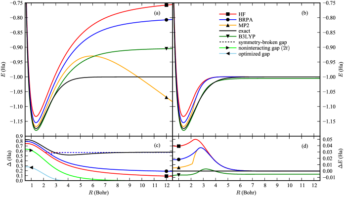
Figure 1: Total energy, $E$, with symmetry (a) preserved and (b) broken, (c) virtual-occupied energy gap, $\Delta$, and (d) error in the symmetry-broken total energy, $\Delta E$, for H₂ as a function of bond length, $R$. The RPA+SOSEX correlation energy is exact for an optimized gap when $R<3.7$.

We consider H_n because it gives us fine control over the number of electrons and also because H₂ is the simplest two-electron molecule with an internal coordinate. The ZDO form of H₂ is an extended Hubbard model with $\alpha=2$ and

$$\mathbf{h}=\scriptsize\left[\begin{array}[]{cccc}\mu&-t&0&0\\ -t&\mu&0&0\\ 0&0&\mu&-t\\ 0&0&-t&\mu\end{array}\right]\normalsize,\ \ \ \mathbf{V}=\scriptsize\left[\begin{array}[]{cccc}U&V&U&V\\ V&U&V&U\\ U&V&U&V\\ V&U&V&U\end{array}\right]\normalsize,$$ (57)

in the notation of Eq. (22). It has a natural pairwise extension to the $n>2$ case. Separate H₂ and H_n Hamiltonians are fit in Appendix B. The H₂ version is fit to reproduce exact, HF, and MP2 total energies. The H_n version is fit to a simple distance-dependent form that gives proper asymptotic behavior. These models have limited transferability, which is a standard caveat of semiempirical modeling with simple Hamiltonian forms.

VI.1 Accuracy of BRPA on H₂

Symmetric dissociation of H₂ is used as a critical test of new electron correlation methods H2_SOSEX ; H2_RPA ; H2_GW . The model in Eq. (57) has simple formulas for HF, MP2, BRPA, and exact energies,

$$E_{\mathrm{HF}} =E_{0}+2(\mu-t)+\tfrac{1}{2}(U+V),$$

$$E_{\mathrm{MP2}} =E_{\mathrm{HF}}-\tfrac{(U-V)^{2}}{16t+8V},\ \ \ E_{\mathrm{BRPA}}=E_{\mathrm{HF}}-\tfrac{(U-V)^{2}}{16t+8U},$$

$$E =E_{\mathrm{HF}}+2t-\sqrt{4t^{2}+\tfrac{1}{4}(U-V)^{2}}.$$ (58)

Dissociation curves are shown in Fig. 1a. BRPA is a uniform improvement over HF but has three times the error of MP2 or B3LYP at equilibrium. These methods fail at dissociation, but BRPA is stable at twice the B3LYP error as MP2 diverges.

RPA+SOSEX total energies are strongly modulated by the choice of mean field. As shown in Fig. 1c, errors in H₂ near equilibrium can be corrected by significantly reducing the gap. This is typical behavior, and the smaller orbital gaps in DFT reference mean fields systematically improve total energies RPArev1 over HF-based calculations RPA3rd . Reducing gaps to reduce errors conflicts with the generalized Koopmans theorem in Eq. (II.3) that requires the BRPA gap to approximate the physical gap. On H₂, BRPA increases the HF gap towards the exact gap, but some methods for calculating excitations such as $GW$ theory decrease the HF gap H2_GW . One possible resolution is to derive an RPA+SOSEX model where orbital energies are not required to approximate electron addition and removal energies, such as by modifying $P_{xy}^{\lambda}(\omega)$ in Eq. (35) with exchange terms Hubbard_SOSEX .

Dissociation failures can be fixed by enabling symmetry breaking in the reference state. As shown in Fig. 1d, the error now peaks at around twice the equilibrium bond length. MP2 now has uniformly less error than BRPA, but BRPA fixes the derivative discontinuity in the MP2 energy surface. Symmetry breaking is needed for size consistency at this level of theory when considering the dissociation of a closed-shell molecule into open-shell fragments. It also serves as a simple model of static correlation. Broken symmetries can be restored with a projection PHF , but the resulting total energy corrections are not size consistent. An accurate, size-consistent model of electron correlation should be able to repair symmetries broken by the reference state accurately but not necessarily exactly.

A single example such as H₂ is not enough to determine error statistics and compare the average errors of total energy methods. However, while errors on a system as important and simple as H₂ remain large, it suffices to discount methods.

Table 1: Leading-order, per-iteration floating-point costs and memory footprints of MP2 and the inner and outer loops of BRPA.

Algorithm	Operations	Memory
1. Conventional MP2	$4\alpha^{3}n^{5}$	$2.5\alpha^{2}n^{2}$
2. Conventional Inner BRPA	$4\alpha^{3}n^{5}$	$2\alpha^{2}n^{3}$
3. Conventional Outer BRPA	$4\alpha^{3}n^{5}$	$2\alpha^{2}n^{3}$
4. Fast MP2	$6\beta_{1}\beta_{2}\beta_{3}\alpha^{2}n^{2}+2\beta_{1}(2\beta_{2}+3\beta_{3}+\gamma)\alpha^{3}n^{3}$	$\beta_{1}\beta_{2}\beta_{3}+(\beta_{1}\beta_{2}+\beta_{1}\beta_{3})\alpha n+(3\beta_{1}+2\beta_{2}+2\beta_{3})\alpha^{2}n^{2}$
5. Fast Inner BRPA	$2\beta_{1}(5\beta_{1}+\gamma)\alpha^{2}n^{2}+12\beta_{1}\alpha^{3}n^{3}$	$2\beta_{1}^{2}+4.5\beta_{1}\alpha^{2}n^{2}$
6. Fast Outer BRPA	$2\beta_{1}^{2}\beta_{2}\beta_{3}\alpha^{2}n^{2}+2(2\beta_{1}+\gamma)\beta_{2}\beta_{3}\alpha^{3}n^{3}$	$2\beta_{1}\beta_{2}\beta_{3}+(\beta_{1}^{2}+2\beta_{1}\beta_{2}+2\beta_{1}\beta_{3}+\beta_{2}\beta_{3})\alpha n+(3\beta_{1}+2\beta_{2}+3\beta_{3})\alpha^{2}n^{2}$

VI.2 Scaling of BRPA on H_n

We benchmark the algorithms in Sec. V on H_n rings, with the intent to produce representative scaling behavior and not necessarily to optimize performance. To this end, we consider only $n=4m+2$ for a closed shell and a finite orbital gap. We use an HF mean field in all calculations to enable the use of common quadratures. The algorithm runtimes are comparable to per-iteration costs and a full self-consistent calculation will have number of iterations as an additional cost multiplier.

The HF orbital gap decreases as $\Delta\approx 2.7n^{-0.83}$. Using the quadrature formulas in Appendix A with errors that are set to $\varepsilon_{Q}=10^{-5}$, the quadrature sizes are observed to increase as

$$\beta_{1} \approx 1.7+2.1\ln n,$$

$$\beta_{2} \approx-0.7+4.1\ln n,$$

$$\beta_{3} \approx 3.3+4.1\ln n.$$ (59)

These are not asymptotic scalings. When the orbital gap falls below a numerical low-energy cutoff, we will add an artificial gap comparable to this cutoff that limits quadrature size.

Benchmarks are measured on a c implementation supplement . The HF Hamiltonian matrix is diagonalized with the dsyev routine in lapack LAPACK . Tensors are contracted with the real dgemm and complex zgemm routines in blas BLAS . A conversion factor from runtimes to operation counts is determined by timing the $2n^{3}$ operations of $n$-by-$n$ matrix-matrix multiplications in dgemm calls for large $n$. Conventional algorithms use real arithmetic, while fast algorithms use complex arithmetic. The increased cost of complex arithmetic is mitigated by using symmetry symmetry_note . $V_{xy}\rho_{y}$ is summed with fftw FFTW . For regular behavior of $\gamma$, we further restrict H_n to $n=2^{p}-2$ and embed $V_{xy}\rho_{y}$ in a cyclic convolution of size $2^{p+1}$. We observe an fftw scaling of

$$\gamma\approx 23+13\ln n.$$ (60)

Other fast summation methods fast_kernel_sum avoid a $\ln n$ prefactor.

Benchmark results are shown in Fig. 2. The runtimes are compared to the model estimates summarized in Table 1. The agreement is good, and all discrepancies can be rationalized. The inBRPAf cost is increased $50\%$ by complex arithmetic symmetry_note . The excess cost of MP2f is caused by zgemm calls with small $\mathcal{O}(\beta_{1})$ matrix dimensions. The excess cost of outBRPAf is caused by subleading-order terms with large prefactors. Fast and conventional calculations agree to $10^{-7}$ Ha in $\sigma_{xy}$.

In the cost model, the crossover between conventional and fast runtimes occurs at $n=62$ for MP2 and $n=422$ for BRPA. As all algorithms have an $\mathcal{O}(\alpha^{3})$ scaling, larger basis sets will not shift the crossover. Other prefactors will but are indicative of realistic values as quadrature sizes are reported oldfastRPA ; VASP_RPA from $16$ to $40$ and the FFT is a standard fast summation method.

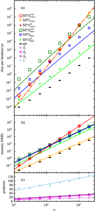
Figure 2: The (a) operation, (b) memory, and (c) prefactor costs of H_n on a single core of an Intel Xeon X5650. Points are measured costs, and the equivalently colored lines are the model costs cost_note . The model conversion factor between operation count and runtime is 10 Gflops.

VII Discussion

A natural continuation of the research in this paper is the extension of the algorithms in Sec. V for implementation in established electronic structure codes. For a Gaussian-orbital code, this means nontrivial overlap matrices between primary basis functions and between pairs of primary basis functions and auxiliary basis functions. It needs an implementation of THC or some other decomposition of $V_{rs}^{pq}$ with a sparse vertex tensor and a Gaussian-compatible FMM CFMM . This combination of features is not yet available in any code. For a planewave-pseudopotential code, algorithms for periodic systems need to be developed. Suitable FFT and grid operations for efficient $V_{rs}^{pq}$ decomposition are widely available in these codes.

An orthogonal direction for continued research is further development of basic algorithms and numerical analysis that improve cubic-scaling correlation models. One such direction is analysis of the slow basis set convergence that is a universal detriment to non-DFT electron correlation models. Another is the development of more accurate correlation models that are restricted to $\mathcal{O}(\alpha^{3}n^{3})$ operations and $\mathcal{O}(\alpha^{2}n^{2})$ memory. These two directions are discussed in more detail below.

VII.1 The operator approximation problem

The $\alpha$ prefactor depends on the choice of basis set. Basis construction is widely considered as a function approximation problem of electron orbitals. It is usually focused on occupied orbitals, their response to perturbations, and low-lying virtual orbitals. Larger $\alpha$ values improve their approximation, while smaller $\alpha$ values reduce costs. The number of virtual orbitals defined by the basis set is also determined by $\alpha$.

Slow basis set convergence manifests in the virtual orbital summations in MP2 and related calculations. Convergence is often accelerated with basis set extrapolation to avoid large $\alpha$ values extrapolation . In wavefunction-based methods, slow convergence is attributed to electron-electron cusps in the wavefunction cusp that are corrected by R12/F12 R12 or Jastrow Jastrow methods. In the fast algorithms in Sec. V, there are only operators and their finite-basis errors instead of summations over virtual orbitals or wavefunction cusps. In the case of a spinless nonrelativistic Hamiltonian, the BRPA operator variables asymptote to

$$G(\vec{x},\vec{y},\omega)\rightarrow\frac{-1}{2\pi|\vec{x}-\vec{y}|},\ \ \ A(\vec{x},\vec{y},\omega)\rightarrow\frac{-\rho(\vec{x},\vec{y})}{2\pi|\vec{x}-\vec{y}|},$$ (61)

as $|\vec{x}-\vec{y}|\rightarrow 0$. These singularities converges slowly with basis set size and are better approximated by functions of $|\vec{x}-\vec{y}|$.

The efficient and accurate representation of $A(\mathbf{x},\mathbf{y},\omega)$ and $G(\mathbf{x},\mathbf{y},\omega)$ is an operator approximation problem. $G(\mathbf{x},\mathbf{y},\omega)$ is the simplest case where we seek to satisfy

$$\int d\mathbf{z}[\omega\delta(\mathbf{x}-\mathbf{z})-f(\mathbf{x},\mathbf{z})]G(\mathbf{z},\mathbf{y},\omega)\approx\delta(\mathbf{x}-\mathbf{y}).$$ (62)

The conventional approach is to approximate $G(\mathbf{x},\mathbf{y},\omega)$ with a sum of pairwise products of basis functions. The possibilities beyond this include basis operators that are added linearly or as pairwise products and the direct modeling of singularities. An operator-based approach can also use spatial localization linear_scaling that does not manifest in molecular orbitals. These ideas form a distinct alternative to orbital function approximation.

VII.2 The cost-restricted electron correlation problem

The BRPA model developed in this paper is in the class of RPA models, but it is derived from BCCD theory. Historically, the mathematical structure of RPA has emerged from multiple theories: resummation of diagrammatic perturbation theory RPA_egas , boson approximation of electron-hole excitation operators RPA_transform , equations-of-motion for ground state annihilation operators RPA_EOM , integration of response functions over interaction strength RPA_AC , integration of Slater determinants over generator variables RPA_GCM , $1/N$ expansion in $N$ interacting copies of the Hilbert space RPA_largeN , total energy functionals of the many-body Green’s function GW , and an adaptation of interaction strength integration to DFT RPA_DFT . This diverse set of theoretical ideas is responsible for the large number of modern RPA variants RPArev1 ; RPArev2 ; RPArev3 . Much like DFT, there is no rigorous delineation on what can be incorporated into an RPA model of electron correlation energy.

The results of this paper suggest a delineation of models based on computational complexity: a cost strictly bound by a scaling of $\mathcal{O}(n^{3})$ operations and $\mathcal{O}(n^{2})$ memory with a limit on the form of allowed approximations. Other approximations such as orbital localization local_MP2 and stochastic sampling MC_MP2 ; MC2_MP2 can further reduce the scaling of MP2-like methods but introduce localization length and number of samples as complications. A critical question is whether or not these cost restrictions are sufficient to enable method development based on the direct approximation of a quantum state as in CC theory or if it is to be confined to the indirect and often empirical development that is characteristic of modern DFT Jacobs_ladder .

VIII Conclusions

The results of this paper cross an important threshold. For the first time, the computational cost of an electron correlation model with a direct connection to an underlying wavefunction has been reduced to the canonical cost of an SCF calculation, $\mathcal{O}(n^{3})$ operations and $\mathcal{O}(n^{2})$ memory, without localization or stochastic approximations. This includes MP2 theory and an RPA+SOSEX approximation of BCCD theory. The new ideas used to achieve this result may also contribute to reducing the cost of more accurate electron correlation models.

Electron correlation models that require $\mathcal{O}(n^{3})$ operations and $\mathcal{O}(n^{2})$ memory could constitute a distinct paradigm with continued development. They are a compromise between the low cost of DFT and the high accuracy of CC theory. For this compromise to be worthwhile, we need to explore the balance between cost and accuracy to identify its fundamental limits.

Appendix A Numerical quadrature

An implementation of the fast MP2 and BRPA algorithms requires numerical quadratures for the integrals appearing in Eqs. (III.2) and (III.2). We restate these integrals and quadratures in a more general notation with explicit summations,

$$\frac{1}{a+a^{\prime}} =\int_{-i\infty}^{i\infty}\frac{dx}{2\pi i}\frac{1}{(a-x)(a^{\prime}+x)}$$

$$\approx\sum_{i=1}^{n_{x}}\frac{w_{i}}{(a-x_{i})(a^{\prime}+x_{i})},\ \ \ a,a^{\prime}\in A,$$

$$\frac{\theta(b,B)\theta(c,C)}{b-c+x} =\oint_{Y}\frac{dy}{2\pi i}\oint_{Z}\frac{dz}{2\pi i}\frac{1}{(b-y)(c-z)(y-z+x)}$$

$$\approx\sum_{i=1}^{n_{y}}\sum_{j=1}^{n_{z}}\frac{W_{ij}(x)}{(b-y_{i})(c-z_{j})},\ \ \ b,c\in B\cup C,$$

$$\theta(s,S) =1\ \ \ \forall s\in S,\ \ \ \theta(s,S)=0\ \ \ \forall s\not\in S.$$ (63)

$A$ is the set of orbital transition energies ($\epsilon_{a}-\epsilon_{i}$), $B$ is the set of virtual orbital energies ($\epsilon_{a}$), $C$ is the set of occupied orbital energies ($\epsilon_{i}$), $X$ is the set of imaginary reals, and $Y$ and $Z$ are closed counterclockwise contours that satisfy

$$B \subset\mathrm{in}(Y),\ \ \ (B+X)\cap\mathrm{in}(Z)=\varnothing,$$

$$C \subset\mathrm{in}(Z),\ \ \ (C-X)\cap\mathrm{in}(Y)=\varnothing,$$ (64)

for interior, $\mathrm{in}(S)=\{ts+(1-t)s^{\prime}:t\in[0,1],s,s^{\prime}\in S\}$, and elemental arithmetic, $S\pm S^{\prime}=\{s\pm s^{\prime}:s\in S,s^{\prime}\in S^{\prime}\}$, set operations. We assume $A=B-C$ and $a>0\ \forall a\in A$.

Eq. (A) is assembled from more elementary quadratures. We split the first integral into two terms with partial fractions,

$$\frac{1}{a+a^{\prime}}=\frac{1}{a+a^{\prime}}\int_{-i\infty}^{i\infty}\frac{dx}{2\pi i}\left[\frac{1}{a-x}-\frac{1}{-a^{\prime}-x}\right],$$ (65)

and fit quadrature to its two terms on a merged domain,

$$\theta(a,A)-\frac{1}{2}=\int_{-i\infty}^{i\infty}\frac{dx}{2\pi i}\frac{1}{a-x}\approx\sum_{i=1}^{n_{x}}\frac{w_{i}}{a-x_{i}},\ \ \ a\in A^{\prime},$$ (66)

for $A^{\prime}=A\cup\{-a:a\in A\}$. For the second integral, we split with partial fractions after performing one of the integrations,

$$\frac{\theta(b,B)\theta(c,C)}{b-c+x} =\frac{\theta(c,C)}{b-c+x}\oint_{Y}\frac{dy}{2\pi i}\left[\frac{1}{b-y}-\frac{1}{c-x-y}\right],$$

$$=\frac{\theta(b,B)}{b-c+x}\oint_{Z}\frac{dz}{2\pi i}\left[\frac{1}{c-z}-\frac{1}{b+x-z}\right],$$

and again fit quadratures to each contour on a merged domain,

$$\theta(b,B) =\oint_{Y}\frac{dy}{2\pi i}\frac{1}{b-y}\approx\sum_{i=1}^{n_{y}}\frac{u_{i}}{b-y_{i}},\ \ \ b\in B^{\prime},$$

$$\theta(c,C) =\oint_{Z}\frac{dz}{2\pi i}\frac{1}{c-z}\approx\sum_{i=1}^{n_{z}}\frac{v_{i}}{c-z_{i}},\ \ \ c\in C^{\prime},$$ (67)

for $B^{\prime}=B\cup(C-X)$ and $C^{\prime}=C\cup(B+X)$. The fits combine to produce the quadrature weight, $W_{ij}(x)=u_{i}v_{j}/(y_{i}-z_{j}+x)$. We assume that the reassembly of these quadratures is stable and leave further error analysis to future work.

We approximate Eq. (66) with a 1-parameter quadrature,

$$\frac{1}{2}\mathrm{sgn}(a^{\prime})\approx\sum_{i=1}^{2n+1}\frac{w^{\prime}_{i}}{a^{\prime}-x^{\prime}_{i}},\ \ \ a^{\prime}\in[-1,-k]\cup[k,1],$$ (68)

for $0<k<1$ and map back to the original quadrature with

$$\scriptsize\begin{bmatrix}w_{i}\\[-2.5pt] x_{i}\\[-2.5pt] a\end{bmatrix}\normalsize=\max(A)\scriptsize\begin{bmatrix}w^{\prime}_{i}\\[-2.5pt] x^{\prime}_{i}\\[-2.5pt] a^{\prime}\end{bmatrix}\normalsize,\ \ \ k=\tfrac{\min(A)}{\max(A)},\ \ \ n_{x}=2n+1.$$ (69)

Zolotarev’s rational approximation of the sign function using Jacobi elliptic functions minimizes the maximum error Zolotarev ,

$$\varepsilon =\tfrac{1}{2}\tfrac{r(k)-r(\kappa)}{r(k)+r(\kappa)},\ \ \ r(x)=\tfrac{1}{x}\prod_{m=1}^{n}\tfrac{x^{2}+f^{2}_{2m-1}}{x^{2}+f^{2}_{2m}},$$

$$f_{m} =k\tfrac{\mathrm{sn}(m\theta,k^{\prime})}{\mathrm{cn}(m\theta,k^{\prime})},\ \ \ w^{\prime}_{1}=\tfrac{1}{r(k)+r(\kappa)}\prod_{m=1}^{n}\tfrac{f_{2m-1}^{2}}{f_{2m}^{2}},$$

$$w^{\prime}_{2m} =w^{\prime}_{2m+1}=\tfrac{1}{2}\tfrac{1}{r(k)+r(\kappa)}\prod_{p=1}^{n}\tfrac{f_{2m}^{2}-f_{2p-1}^{2}}{f_{2m}^{2}-f_{2p}^{2}(1-\delta_{pm})},$$

$$x^{\prime}_{1} =0,\ \ \ x^{\prime}_{2m}=-x^{\prime}_{2m+1}=if_{2m},$$

$$k^{\prime} =\sqrt{1-k^{2}},\ \ \ \kappa=\tfrac{k}{\mathrm{dn}(\theta,k^{\prime})},\ \ \ \theta=\tfrac{K^{\prime}(k)}{2n+1}.$$ (70)

$\varepsilon$ is the maximum error, which decays exponentially in $n$ with an exponent of $2\pi K(k)/K^{\prime}(k)$ that asymptotes to $\pi^{2}/\ln(4/k)$ in the $k\rightarrow 0$ limit sgn_decay . $\mathrm{sn}(u,k)$, $\mathrm{cn}(u,k)$, and $\mathrm{dn}(u,k)$ are Jacobi elliptic functions. $K(k)$ and $iK^{\prime}(k)$ are their quarter periods.

We approximate Eq. (A) with a 1-parameter quadrature,

$$\mathrm{sgn}(\mathrm{Re}(b^{\prime}))\approx\sum_{i=1}^{2n+1}\frac{u^{\prime}_{i}}{b^{\prime}-y^{\prime}_{i}},\ \ \ b^{\prime}\in X\cup[\lambda,1],$$ (71)

for $0<\lambda<1$ and map back to the original quadratures with

$$\scriptsize\begin{bmatrix}u_{i}\\[-2.5pt] y_{i}-\max(C)\\[-2.5pt] b-\max(C)\end{bmatrix}\normalsize=\left[\max(B)-\max(C)\right]\scriptsize\begin{bmatrix}u^{\prime}_{i}\\[-2.5pt] y^{\prime}_{i}\\[-2.5pt] b^{\prime}\end{bmatrix}\normalsize,$$

$$\lambda=\tfrac{\min(B)-\max(C)}{\max(B)-\max(C)},\ \ \ n_{y}=2n+1,\ \ \ \mathrm{or}$$

$$\scriptsize\begin{bmatrix}v_{i}\\[-2.5pt] z_{i}-\min(B)\\[-2.5pt] c-\min(B)\end{bmatrix}\normalsize=\left[\min(C)-\min(B)\right]\scriptsize\begin{bmatrix}u^{\prime}_{i}\\[-2.5pt] y^{\prime}_{i}\\[-2.5pt] b^{\prime}\end{bmatrix}\normalsize,$$

$$\lambda=\tfrac{\max(C)-\min(B)}{\min(C)-\min(B)},\ \ \ n_{z}=2n+1.$$ (72)

The interiors of $B+X$ and $C-X$ are omitted from Eq. (71) by the maximum modulus principle. We map from Eq. (68) to Eq. (71) with a shift of $\mathrm{sgn}(a^{\prime})$ by $1/2$ and a transformation,

$$a^{\prime}=\tfrac{(1+k)(b^{\prime})^{2}-2k}{2-(1+k)(b^{\prime})^{2}},\ \ \ k=\tfrac{\lambda^{2}}{2-\lambda^{2}+2\sqrt{1-\lambda^{2}}}.$$ (73)

The rational transformation creates a reflection of the original contour about the imaginary axis and doubles the number of poles. We remove the new contour and its poles leaving

$$u^{\prime}_{i}=\tfrac{w^{\prime}_{i}}{y^{\prime}_{i}}\tfrac{1-k}{(1+k)(1+x^{\prime}_{i})^{2}},\ \ \ y^{\prime}_{i}=\sqrt{2\tfrac{k+x^{\prime}_{i}}{(1+k)(1+x^{\prime}_{i})}}.$$ (74)

Empirically, we observe that the maximum error is twice $\varepsilon$ in Eq. (A). This approximant does not minimize the maximum error exactly, but we conjecture that the exponential decay rate of the error with $n$ is optimal.

Appendix B Semiempirical H_n model

To solve the semiempirical H₂ model in Eq. (57), we use a family of reference orbitals parameterized by $\theta$,

$$\boldsymbol{\phi}_{a} =\scriptsize\begin{bmatrix}\sin\theta\\[-2.5pt] -\cos\theta\\[-2.5pt] 0\\[-2.5pt] 0\end{bmatrix}\normalsize,\ \ \ \boldsymbol{\phi}_{b}=\scriptsize\begin{bmatrix}0\\[-2.5pt] 0\\[-2.5pt] -\cos\theta\\[-2.5pt] \sin\theta\end{bmatrix}\normalsize,$$

$$\boldsymbol{\phi}_{i} =\scriptsize\begin{bmatrix}\cos\theta\\[-2.5pt] \sin\theta\\[-2.5pt] 0\\[-2.5pt] 0\end{bmatrix}\normalsize,\ \ \ \boldsymbol{\phi}_{j}=\scriptsize\begin{bmatrix}0\\[-2.5pt] 0\\[-2.5pt] \sin\theta\\[-2.5pt] \cos\theta\end{bmatrix}\normalsize,$$ (75)

where $\{i,j\}$ label the two occupied orbitals and $\{a,b\}$ label the two virtual orbitals. The nonzero matrix elements are

$$h_{i}^{i} =h_{j}^{j}=\mu-t\sin 2\theta,$$

$$h_{a}^{a} =h_{b}^{b}=\mu+t\sin 2\theta,\ \ \ h_{a}^{i}=h_{b}^{j}=t\cos 2\theta,$$

$$V_{pp}^{pp} =V_{aj}^{aj}=V_{bi}^{bi}=U-\tfrac{1}{2}(U-V)(\sin 2\theta)^{2},$$

$$V_{ai}^{ai} =V_{bj}^{bj}=V_{ab}^{ab}=V_{ij}^{ij}=V+\tfrac{1}{2}(U-V)(\sin 2\theta)^{2},$$

$$V_{aa}^{ii} =V_{bb}^{jj}=-V_{ab}^{ij}=\tfrac{1}{2}(U-V)(\sin 2\theta)^{2},$$

$$V_{ab}^{ib} =V_{ai}^{ii}=V_{ba}^{ja}=V_{bj}^{jj}=-V_{aa}^{ia}=-V_{aj}^{ij}$$

$$=-V_{bb}^{jb}=-V_{bi}^{ji}=\tfrac{1}{4}(U-V)\sin 4\theta,$$ (76)

with symmetric extensions for ${}_{p}^{q}\Leftrightarrow\,\!_{q}^{p}$ and ${}_{rs}^{pq}\Leftrightarrow\,\!_{sr}^{qp}$.

The BCCD total energy in terms of $T=T_{ij}^{ab}$ is

$$E =E_{0}+2(\mu-t\sin 2\theta)+V$$

$$\ \ \ +\tfrac{1}{2}(U-V)(1-T)(\sin 2\theta)^{2}.$$ (77)

The mean field equations are an orbital energy difference, $\Delta$, and a coupling between occupied and virtual orbitals,

$$\Delta =2t\sin 2\theta+U-(U-V)(1-T)(\sin 2\theta)^{2},$$ (78a)

$$0 =[t(1+T)-\tfrac{1}{2}(U-V)(1-T)\sin 2\theta]\cos 2\theta.$$ (78b)

These are the complete HF equations if $T=0$. There are up to two solutions: a nonsymmetric state and a symmetric state for $\sin 2\theta=1$. In BCCD theory, $T$ is the solution to Eq. (II.1),

$$0=2(\Delta-U)T-\tfrac{1}{2}(U-V)(1-4T+3T^{2})(\sin 2\theta)^{2}.$$ (79)

The RPA Riccati equation in Eq. (14) similarly reduces to

$$0=2\Delta T-\tfrac{1}{2}(U-V)(1-4T+4T^{2})(\sin 2\theta)^{2},$$ (80)

which simplifies the 4-by-4 matrix equation for $T_{ij}^{ab}$ to a direct condition on $T$ by exploiting matrix symmetries.

For $\theta=\tfrac{1}{4}\pi$, the quadratic formula is used to solve for $T$,

$$T(\mathrm{exact}) =\sqrt{\left[\tfrac{4t}{U-V}\right]^{2}+1}-\tfrac{4t}{U-V}\leq 1,$$

$$T(\mathrm{RPA}) =\tfrac{1}{2}\left[1+\tfrac{\Delta}{U-V}\right]-\tfrac{1}{2}\sqrt{\left[1+\tfrac{\Delta}{U-V}\right]^{2}-1}\leq\tfrac{1}{2},$$

$$T(\mathrm{BRPA}) =\tfrac{1}{4}\tfrac{U-V}{U+2t}\leq\tfrac{1}{4}.$$ (81)

The bounds on $T$ are achieved at dissociation and for $\Delta=0$ in the RPA case, which deviates from the BRPA value of $\Delta$. The approximations change the fundamental range of $T$ values.

We determine one set of parameters for the semiempirical model by solving for $\{t,\mu,V\}$ given $\{E_{\mathrm{HF}},E_{\mathrm{MP2}},E\}$ at $\theta=\tfrac{1}{4}\pi$,

$$E_{1} =4(E_{\mathrm{HF}}-E_{\mathrm{MP2}})(E_{\mathrm{HF}}-E)/(E_{\mathrm{MP2}}-E),$$

$$V =U+E_{1}\left[1-\sqrt{1+(E-E_{\mathrm{HF}}+2U)/E_{1}}\right],$$

$$t =\tfrac{1}{16}(U-V)^{2}/(E_{\mathrm{HF}}-E)-\tfrac{1}{4}(E_{\mathrm{HF}}-E),$$

$$\mu =t-\tfrac{1}{4}(U+V)-\tfrac{1}{2}(E_{0}-E_{\mathrm{HF}}).$$ (82)

where $E_{0}=1/R$ for interatomic separation $R$ and $U$ is set to its value at the dissociation limit, $U=0.5695$. The H₂ data is generated in gaussian09 using the cc-pV6Z basis G09 . The data and parameters are compiled in Table 2.

We consider an extension to H_n having a pairwise form,

$$E_{0} =\frac{1}{2}\sum_{x\neq y}\frac{1}{R_{xy}},\ \ \ x,y\in\{1,\cdots,n\},$$

$$h_{(x\sigma)(y\sigma^{\prime})} =-\delta_{\sigma\sigma^{\prime}}\delta_{xy}\tfrac{1}{2}-\delta_{\sigma\sigma^{\prime}}(1-\delta_{xy})t(R_{xy})$$

$$\ \ \ +\delta_{\sigma\sigma^{\prime}}\delta_{xy}\sum_{z\neq x}\Delta\mu(R_{xz}),$$

$$V_{(x\sigma)(y\sigma^{\prime})} =\delta_{xy}0.5695+(1-\delta_{xy})V(R_{xy}),$$ (83)

with spin indices, $\sigma\in\{\uparrow,\downarrow\}$, and interatomic distances, $R_{xy}$. Such a simple model will have limited transferability and care is required in fitting the parameter functions.

For simplicity, we restrict the scaling study to uniform H_n rings that obey Hückel’s rule, $n=4m+2$. Here, $R_{xy}$ is

$$R_{xy}=R\sqrt{\left[1-\cos\left(\tfrac{2\pi(x-y)}{n}\right)\right]\Big{/}\left[1-\cos\left(\tfrac{2\pi}{n}\right)\right]},$$ (84)

for nearest-neighbor distance $R$. Spin and spatial symmetries simplify the normalized orbitals to

$$\phi_{(1\sigma)(x\sigma^{\prime})} =\delta_{\sigma\sigma^{\prime}}\sqrt{\tfrac{1}{n}},\ \ \ \phi_{(n\sigma)(x\sigma^{\prime})}=\delta_{\sigma\sigma^{\prime}}\sqrt{\tfrac{1}{n}}(-1)^{x},$$

$$\phi_{(2m\sigma)(x\sigma^{\prime})} =\delta_{\sigma\sigma^{\prime}}\sqrt{\tfrac{2}{n}}\sin\left(\tfrac{2\pi mx}{n}\right),\ \ \ 1\leq m\leq\tfrac{n}{2}-1,$$

$$\phi_{(2m+1\sigma)(x\sigma^{\prime})} =\delta_{\sigma\sigma^{\prime}}\sqrt{\tfrac{2}{n}}\cos\left(\tfrac{2\pi mx}{n}\right),$$ (85)

The density matrix sums to form the Dirichlet kernel,

$$\rho_{(x\sigma)(y\sigma^{\prime})}=\frac{1}{n}\delta_{\sigma\sigma^{\prime}}\frac{\sin(\pi(x-y)/2)}{\sin(\pi(x-y)/n)}.$$ (86)

We use the HF energy of H₆, $E_{6}$, for fitting to these H_n rings. $R$ is optimized by minimizing the HF total energy.

We fit Eq. (B) to $\{E_{\mathrm{HF}},E_{6},E\}$ with exponential forms for $t(R)$, $\Delta\mu(R)$, and $V(R)$ plus long-range asymptotic corrections for $\Delta\mu(R)$ and $V(R)$ with the form of an electrostatic potential between a 1s Slater-type orbital and point charge. With 6 free parameters, the result of this nonlinear least-squares fit is

$$V(R) =0.304\exp(-0.616R)+[1-\exp(-0.616R)]/R,$$

$$\Delta\mu(R) =0.000\exp(-1.235R)-[1-\exp(-1.235R)]/R,$$

$$t(R) =0.206\exp(-0.383R),$$ (87)

with a root-mean-square error of $0.008$ Ha/atom. The primed parameters calculated from Eq. (B) are given in Table 2. In this model, H_n rings have optimal $R$ values between $1.36$ and $1.89$ and their HF energy asymptotes to $-0.527$ Ha/atom.

Table 2: Total energies (of H₂ unless otherwise stated) and model parameters (in Hartrees) at nearest-neighbor interatomic separation $R$ (in Bohrs).

$R$	HF(H6)	HF	B3LYP	UB3LYP	MP2	exact	$\mu$	$\mu^{\prime}$	$t$	$t^{\prime}$	$U$ & $U^{\prime}$	$V$	$V^{\prime}$
$0.5$	$3.35175$	$-0.48666$	$-0.53368$	$-0.53368$	$-0.52150$	$-0.52641$	$-1.09542$	$-1.42142$	$0.31841$	$0.17010$	$0.56950$	$0.11250$	$0.75358$
$0.7$	$-0.27931$	$-0.88259$	$-0.92834$	$-0.92834$	$-0.91676$	$-0.92184$	$-1.01031$	$-1.32677$	$0.31680$	$0.15756$	$0.56950$	$0.11662$	$0.69790$
$0.9$	$-1.86432$	$-1.04433$	$-1.08972$	$-1.08972$	$-1.07811$	$-1.08348$	$-0.93969$	$-1.24548$	$0.31076$	$0.14594$	$0.56950$	$0.12141$	$0.64749$
$1.1$	$-2.62333$	$-1.11045$	$-1.15616$	$-1.15616$	$-1.14410$	$-1.14991$	$-0.88345$	$-1.17541$	$0.30041$	$0.13518$	$0.56950$	$0.12688$	$0.60180$
$1.3$	$-2.99665$	$-1.13202$	$-1.17854$	$-1.17854$	$-1.16578$	$-1.17221$	$-0.84003$	$-1.11478$	$0.28621$	$0.12521$	$0.56950$	$0.13300$	$0.56036$
$1.5$	$-3.17349$	$-1.13137$	$-1.17909$	$-1.17909$	$-1.16546$	$-1.17273$	$-0.80743$	$-1.06210$	$0.26887$	$0.11598$	$0.56950$	$0.13964$	$0.52271$
$1.7$	$-3.24462$	$-1.11934$	$-1.16858$	$-1.16858$	$-1.15399$	$-1.16233$	$-0.78364$	$-1.01617$	$0.24918$	$0.10742$	$0.56950$	$0.14664$	$0.48849$
$1.9$	$-3.25702$	$-1.10160$	$-1.15262$	$-1.15262$	$-1.13702$	$-1.14673$	$-0.76666$	$-0.97595$	$0.22810$	$0.09950$	$0.56950$	$0.15375$	$0.45734$
$2.1$	$-3.23641$	$-1.08123$	$-1.13425$	$-1.13425$	$-1.11764$	$-1.12904$	$-0.75476$	$-0.94059$	$0.20649$	$0.09216$	$0.56950$	$0.16070$	$0.42896$
$2.3$	$-3.19745$	$-1.05996$	$-1.11519$	$-1.11519$	$-1.09758$	$-1.11105$	$-0.74644$	$-0.90939$	$0.18512$	$0.08537$	$0.56950$	$0.16727$	$0.40307$
$2.5$	$-3.14877$	$-1.03878$	$-1.09640$	$-1.09640$	$-1.07784$	$-1.09380$	$-0.74049$	$-0.88175$	$0.16459$	$0.07907$	$0.56950$	$0.17324$	$0.37942$
$3.0$	$-3.01377$	$-0.98932$	$-1.05352$	$-1.05444$	$-1.03302$	$-1.05718$	$-0.73048$	$-0.82513$	$0.11939$	$0.06529$	$0.56950$	$0.18470$	$0.32871$
$3.5$	$-2.88444$	$-0.94687$	$-1.01831$	$-1.02916$	$-0.99677$	$-1.03171$	$-0.72172$	$-0.78192$	$0.08458$	$0.05391$	$0.56950$	$0.19054$	$0.28783$
$4.0$	$-2.77154$	$-0.91161$	$-0.99060$	$-1.01666$	$-0.96934$	$-1.01625$	$-0.71169$	$-0.74821$	$0.05929$	$0.04452$	$0.56950$	$0.19123$	$0.25460$
$4.5$	$-2.67665$	$-0.88272$	$-0.96928$	$-1.01074$	$-0.94992$	$-1.00788$	$-0.70042$	$-0.72136$	$0.04140$	$0.03676$	$0.56950$	$0.18795$	$0.22734$
$5.0$	$-2.59835$	$-0.85919$	$-0.95312$	$-1.00788$	$-0.93749$	$-1.00369$	$-0.68868$	$-0.69958$	$0.02880$	$0.03035$	$0.56950$	$0.18205$	$0.20478$
$5.5$	$-2.53436$	$-0.84008$	$-0.94096$	$-1.00646$	$-0.93098$	$-1.00170$	$-0.67710$	$-0.68161$	$0.01988$	$0.02506$	$0.56950$	$0.17464$	$0.18595$
$6.0$	$-2.48232$	$-0.82454$	$-0.93187$	$-1.00573$	$-0.92941$	$-1.00078$	$-0.66608$	$-0.66657$	$0.01352$	$0.02069$	$0.56950$	$0.16651$	$0.17008$
$7.0$	$-2.40582$	$-0.80152$	$-0.92003$	$-1.00513$	$-0.93770$	$-1.00017$	$-0.64641$	$-0.64283$	$0.00567$	$0.01411$	$0.56950$	$0.15010$	$0.14502$
$8.0$	$-2.35516$	$-0.78604$	$-0.91341$	$-1.00496$	$-0.95637$	$-1.00004$	$-0.63013$	$-0.62499$	$0.00157$	$0.00962$	$0.56950$	$0.13524$	$0.12630$
$10.0$	$-2.29692$	$-0.76768$	$-0.90729$	$-1.00489$	$-1.00903$	$-1.00000$	$-0.60596$	$-0.60000$	$-0.00176$	$0.00447$	$0.56950$	$0.11195$	$0.10043$
$12.0$	$-2.26638$	$-0.75758$	$-0.90475$	$-1.00488$	$-1.06870$	$-1.00000$	$-0.58946$	$-0.58333$	$-0.00272$	$0.00208$	$0.56950$	$0.09564$	$0.08347$
$16.0$	$-2.23446$	$-0.74655$	$-0.90242$	$-1.00488$	$-1.19169$	$-1.00000$	$-0.56858$	$-0.56250$	$-0.00300$	$0.00045$	$0.56950$	$0.07473$	$0.06251$
$32.0$	$-2.18483$	$-0.73088$	$-0.89929$	$-1.00488$	$-1.70376$	$-1.00000$	$-0.53588$	$-0.53125$	$-0.00231$	$0.00000$	$0.56950$	$0.04056$	$0.03125$
$64.0$	$-2.16530$	$-0.72307$	$-0.89772$	$-1.00488$	$-2.75324$	$-1.00000$	$-0.51848$	$-0.51562$	$-0.00142$	$0.00000$	$0.56950$	$0.02134$	$0.01563$
$\infty$	$-2.14577$	$-0.71526$	$-0.89616$	$-1.00488$	$-\infty$	$-1.00000$	$-0.50000$	$-0.50000$	$0.00000$	$0.00000$	$0.56950$	$0.00000$	$0.00000$

References

• (1) A. Szabo and N. S. Ostlund, Modern Quantum Chemistry: Introduction to Advanced Electronic Structure Theory (Dover, New York, 1996).
• (2) P. Hohenberg and W. Kohn, Phys. Rev. 136, B864 (1964).
• (3) W. Kohn and L. J. Sham, Phys. Rev. 140, A1133 (1965).
• (4) J. P. Perdew and A. Zunger, Phys. Rev. B 23, 5048 (1981).
• (5) P. R. Briddon and M. J. Rayson, Phys. Status Solidi B 248, 1309 (2011).
• (6) R. J. Bartlett and M. Musiał, Rev. Mod. Phys. 79, 291 (2007).
• (7) G. E. Scuseria, T. M. Henderson, and D. C. Sorensen, J. Chem. Phys. 129, 231101 (2008).
• (8) F. Furche, J. Chem. Phys. 129, 114105 (2008).
• (9) H. Eshuis, J. Yarkony, and F. Furche, J. Chem. Phys. 132, 234114 (2010).
• (10) A. Grüneis, M. Marsman, J. Harl, L. Schimka, and G. Kresse, J. Chem. Phys. 131, 154115 (2009).
• (11) D. M. Ceperley and B. J. Alder, Phys. Rev. Lett. 45, 566 (1980).
• (12) D. L. Freeman, Phys. Rev. B 15, 5512 (1977).
• (13) J. Paier, B. G. Janesko, T. M. Henderson, G. E. Scuseria, A. Grüneis, and G. Kresse, J. Chem. Phys. 132, 094103 (2010); 133, 179902 (2010).
• (14) A. Heßelmann, J. Chem. Phys. 134, 204107 (2011).
• (15) X. Ren, P. Rinke, G. E. Scuseria, and M. Scheffler, Phys. Rev. B 88, 035120 (2013).
• (16) J. Paier, X. Ren, P. Rinke, G. E. Scuseria, A. Grüneis, G. Kresse, and M. Scheffler, New J. Phys. 14, 043002 (2012).
• (17) C. Van Alsenoy, J. Comput. Chem. 9, 620 (1988).
• (18) L. Greengard and V. Rokhlin, J. Comput. Phys. 73, 325 (1987).
• (19) J. Almlöf, Chem. Phys. Lett. 181, 319 (1991).
• (20) R. K. Nesbet, Phys. Rev. 109, 1632 (1958).
• (21) L. Z. Stolarczyk and H. J. Monkhorst, Int. J. Quantum Chem., Symp. 26, 267 (1984).
• (22) L. Goerigkab and S. Grimme, Phys. Chem. Chem. Phys. 13, 6670 (2011).
• (23) A. J. Cohen, P. Mori-Sánchez, and W. Yang, Chem. Rev. 112, 289 (2012).
• (24) T. Koopmans, Physica 1, 104 (1934). (in German)
• (25) B. P. Molinari, SIAM J. Control 11, 262 (1973).
• (26) T. N. Lan and T. Yanai, J. Chem. Phys. 138, 224108 (2013).
• (27) Y. Akinaga, Y. Kawashima, and S. Ten-no, Chem. Phys. Lett. 506, 276 (2011).
• (28) I. Lindgren and S. Salomonson, Int. J. Quantum Chem. 90, 294 (2002).
• (29) L. Hedin, Phys. Rev. 139, A796 (1965).
• (30) R. M. Parrish, E. G. Hohenstein, T. J. Martínez, and C. D. Sherrill, J. Chem. Phys. 137, 224106 (2012).
• (31) H. Koch, A. Sánchez de Merás, and T. B. Pedersen, J. Chem. Phys. 118, 9481 (2003).
• (32) T. J. Martínez and E. A. Carter, J. Chem. Phys. 100, 3631 (1994).
• (33) F. Weigend, A. Köhn, and C. Hättig, J. Chem. Phys. 116, 3175 (2002).
• (34) P. E. Blöchl, Phys. Rev. B 50, 17953 (1994).
• (35) J. Harl, L. Schimka, and G. Kresse, Phys. Rev. B 81, 115126 (2010). The $\alpha$ values are generated by vasp using the reported geometries and planewave cutoffs. For an energy cutoff $E$ in Ha and a volume per electron $V$ in Bohr, $\alpha\approx V(2E)^{3/2}/(3\pi^{2})$ using basic accounting of planewaves inside a cubic unit cell in real space and a spherical Fermi sea in momentum space.
• (36) L. Lin, J. Lu, L. Ying, and W. E, Chinese Ann. Math. B 30, 729 (2009).
• (37) A. Takatsuka, S. Ten-no, and W. Hackbusch, J. Chem. Phys. 129, 044112 (2008).
• (38) S. A. Goreinov, E. E. Tyrtyshnikov , and N. L. Zamarashkin, Linear Algebra Appl. 261, 1 (1997).
• (39) C. A. White, B. G. Johnson, P. M.W. Gill, and M. Head-Gordon, Chem. Phys. Lett. 230, 8 (1994).
• (40) J. Paier, R. Hirschl, M. Marsman, and G. Kresse, J. Chem. Phys. 122, 234102 (2005).
• (41) B. Shanker and H. Huang, J. Comput. Phys. 226, 732 (2007).
• (42) R. D. Skeel, I. Tezcan, and D. J. Hardy, J. Comput. Chem. 23, 673 (2002).
• (43) S. Börm, L. Grasedyck, and W. Hackbusch, Eng. Anal. Bound. Elem. 27, 405 (2003).
• (44) G. Jansen, R.-F. Liu, and J. G. Ángyán, J. Chem. Phys. 133, 154106 (2010).
• (45) M. Feyereisen, G. Fitzgerald, and A. Komornicki, Chem. Phys. Lett. 208, 359 (1993).
• (46) E. G. Hohenstein, R. M. Parrish, and T. J. Martínez, J. Chem. Phys. 137, 044103 (2012).
• (47) M. Häser, Theor. Chim. Acta 87, 147 (1993).
• (48) E. G. Hohenstein, R. M. Parrish, C. D. Sherrill, and T. J. Martínez, J. Chem. Phys. 137, 221101 (2012).
• (49) I. Fischer-Hjalmars, J. Chem. Phys. 42, 1962 (1965).
• (50) W. Thiel, J. Am. Chem. Soc. 103, 1413 (1981).
• (51) T. M. Henderson and G. E. Scuseria, Mol. Phys. 108, 2511 (2010).
• (52) P. Mori-Sánchez, A. J. Cohen, and W. Yang, Phys. Rev. A 85, 042507 (2012).
• (53) F. Caruso, D. R. Rohr, M. Hellgren, X. Ren, P. Rinke, A. Rubio, and M. Scheffler, Phys. Rev. Lett. 110, 146403 (2013).
• (54) A. Heßelmann and A. Görling, Mol. Phys. 109, 2473 (2011).
• (55) J. Hubbard, Proc. R. Soc. A 243, 336 (1957).
• (56) C. A. Jiménez-Hoyos, T. M. Henderson, T. Tsuchimochi, and G. E. Scuseria, J. Chem. Phys. 136, 164109 (2012).
• (57) See the supplementary material at http://arxiv.org/e-print/1303.3847 for a c implementation of the algorithms in Sec. V.
• (58) E. Anderson, Z. Bai, C. Bischof, S. Blackford, J. Demmel, J. Dongarra, J. Du Croz, A. Greenbaum, S. Hammarling, A. McKenney, and D. Sorensen, LAPACK Users’ Guide, Third Edition (SIAM, Philadelphia, 1999).
• (59) J. J. Dongarra, J. Du Croz, I. S. Duff, and S. Hammarling, ACM Trans. Math. Soft. 16, 1 (1990).
• (60) In inBRPAf, tensors of the form $Z_{f}^{e}$ and $Z_{xy}^{e}$ have symmetries $Z_{f}^{\overline{e}}=(Z_{\overline{f}}^{e})^{*}$ and $Z_{xy}^{\overline{e}}=(Z_{xy}^{e})^{*}$. MP2f contains these symmetries and adds $Z_{x}^{\overline{e}\underline{p}}=\left(Z_{x}^{e\underline{p}^{*}}\right)^{*}$, $Z_{xy}^{\underline{p}^{*}0}=\left(Z_{xy}^{\underline{p}0}\right)^{*}$, and $Z_{\underline{a}\underline{i}}^{\overline{e}}=\left(Z_{\underline{a}^{*}\underline{i}^{*}}^{e}\right)^{*}$. outBRPAf contains these symmetries and adds $Z_{x}^{\underline{a}^{*}\underline{i}}=\left(Z_{x}^{\underline{a}\underline{i}^{*}}\right)^{*}$. Only half the entries of these symmetric tensors need to be stored and calculated, which halves the memory and operation counts. Complex arithmetic doubles memory usage and FFT runtimes and triples matrix multiplication runtimes over real arithmetic. The additional cost of complex arithmetic is mitigated for all the operations except matrix multiplication (zgemm), which is reduced to 1.5 times the cost model.
• (61) M. Frigo and S. G. Johnson, Proc. IEEE 93, 216 (2005).
• (62) The leading-order cost model assumes that all parameters are much larger than one, which is false for $\alpha=2$. We correct the conventional algorithm costs with $\alpha^{3}\rightarrow\alpha(\alpha-1)^{2}$ for the operation counts, $3\alpha^{2}\rightarrow 3\alpha^{2}+4\alpha-2$ for the MP2 memory cost, and $\alpha^{2}\rightarrow\alpha(\alpha-1)$ for both BRPA memory costs.
• (63) D. G. Truhlar, Chem. Phys. Lett. 294, 45 (1998).
• (64) T. Kato, Commun. Pure Appl. Math. 10, 151 (1957).
• (65) L. Kong , F. A. Bischoff , and E. F. Valeev, Chem. Rev. 112, 75 (2012).
• (66) N. D. Drummond, M. D. Towler, and R. J. Needs, Phys. Rev. B 70, 235119 (2004).
• (67) S. Goedecker, Rev. Mod. Phys. 71, 1085 (1999).
• (68) M. Gell-Mann and K. A. Brueckner, Phys. Rev. 106, 364 (1957).
• (69) K. Sawada, Phys. Rev. 106, 372 (1957).
• (70) M. Baranger, Phys. Rev. 120, 957 (1960).
• (71) A. D. McLachlan and M. A. Ball, Rev. Mod. Phys. 36, 844 (1964).
• (72) B. Jancovici and D. H. Schiff, Nucl. Phys. 58, 678 (1964).
• (73) A. J. Glick, H. J. Lipkin, and N. Meshkov, Nucl. Phys. 62, 211 (1965).
• (74) J. Harris and R. O. Jones, J. Phys. F 4, 1170 (1974).
• (75) H. Eshuis, J. E. Bates, and F. Furche, Theor. Chem. Acc. 131, 1084 (2012).
• (76) X. Ren, P. Rinke, C. Joas, and M. Scheffler, J. Mater. Sci. 47, 7447 (2012).
• (77) P. Y. Ayala and G. E. Scuseria, J. Chem. Phys. 110, 3660 (1999).
• (78) S. Y. Willow, K. S. Kim, and S. Hirata, J. Chem. Phys. 137, 204122 (2012).
• (79) D. Neuhauser, E. Rabani, and R. Baer, J. Chem. Theory Comput. 9, 24 (2013).
• (80) J. P. Perdew and K. Schmidt, AIP Conf. Proc. 577, 1 (2001).
• (81) E. I. Zolotarev, Zap. Imp. Akad. Nauk, St. Petersburg 30, 5 (1877); reprinted in Collected works (Izdat. Akad. Nauk SSSR, Leningrad, 1932), Vol. 2, pp. 1-59. (in Russian)
• (82) A. A. Gončar, Math. USSR Sb. 7, 623 (1969).
• (83) M. J. Frisch, G. W. Trucks, H. B. Schlegel, G. E. Scuseria, M. A. Robb, J. R. Cheeseman, G. Scalmani, V. Barone, B. Mennucci, G. A. Petersson, H. Nakatsuji, M. Caricato, X. Li, H. P. Hratchian, A. F. Izmaylov, J. Bloino, G. Zheng, J. L. Sonnenberg, M. Hada, M. Ehara, K. Toyota, R. Fukuda, J. Hasegawa, M. Ishida, T. Nakajima, Y. Honda, O. Kitao, H. Nakai, T. Vreven, J. A. Montgomery, Jr., J. E. Peralta, F. Ogliaro, M. Bearpark, J. J. Heyd, E. Brothers, K. N. Kudin, V. N. Staroverov, R. Kobayashi, J. Normand, K. Raghavachari, A. Rendell, J. C. Burant, S. S. Iyengar, J. Tomasi, M. Cossi, N. Rega, J. M. Millam, M. Klene, J. E. Knox, J. B. Cross, V. Bakken, C. Adamo, J. Jaramillo, R. Gomperts, R. E. Stratmann, O. Yazyev, A. J. Austin, R. Cammi, C. Pomelli, J. W. Ochterski, R. L. Martin, K. Morokuma, V. G. Zakrzewski, G. A. Voth, P. Salvador, J. J. Dannenberg, S. Dapprich, A. D. Daniels, Ö. Farkas, J. B. Foresman, J. V. Ortiz, J. Cioslowski, and D. J. Fox, gaussian 09, Revision C.01, Gaussian, Inc., Wallingford CT, 2009.