Asymptotic properties of some
minor-closed classes of graphs

Abstract.

Let $\mathcal{A}$ be a minor-closed class of labelled graphs, and let $\mathcal{G}_{n}$ be a random graph sampled uniformly from the set of $n$-vertex graphs of $\mathcal{A}$. When $n$ is large, what is the probability that $\mathcal{G}_{n}$ is connected? How many components does it have? How large is its biggest component? Thanks to the work of McDiarmid and his collaborators, these questions are now solved when all excluded minors are 2-connected.

Using exact enumeration, we study a collection of classes $\mathcal{A}$ excluding non-2-connected minors, and show that their asymptotic behaviour may be rather different from the 2-connected case. This behaviour largely depends on the nature of dominant singularity of the generating function $C(z)$ that counts connected graphs of $\mathcal{A}$. We classify our examples accordingly, thus taking a first step towards a classification of minor-closed classes of graphs. Furthermore, we investigate a parameter that has not received any attention in this context yet: the size of the root component. It follows non-gaussian limit laws (beta and gamma), and clearly deserves a systematic investigation.

1. Introduction

We consider simple graphs on the vertex set $\{1,\ldots,n\}$. A set of graphs is a class if it is closed under isomorphisms. A class of graphs $\mathcal{A}$ is minor-closed if any minor of a graph of $\mathcal{A}$ is in $\mathcal{A}$. To each such class one can associate its set $\mathcal{E}$ of excluded minors: an (unlabelled) graph is excluded if its labelled versions do not belong to $\mathcal{A}$, but the labelled versions of each of its proper minors belong to $\mathcal{A}$. A remarkable result of Robertson and Seymour states that $\mathcal{E}$ is always finite [32]. We say that the graphs of $\mathcal{A}$ avoid the graphs of $\mathcal{E}$. We refer to [6] for a study of the possible growth rates of minor-closed classes.

Figure 1. A zoo of graphs. Top: the 3-star, the triangle $K_{3}$, the bowtie and the diamond. Bottom: A caterpillar and the 4-spoon (a $k$-spoon consists of a “handle” formed of $k$ edges, to which a triangle is attached).

For a minor-closed class $\mathcal{A}$, we study the asymptotic properties of a random graph $\mathcal{G}_{n}$ taken uniformly in $\mathcal{A}_{n}$, the set of graphs of $\mathcal{A}$ having $n$ vertices: what is the probability $p_{n}$ that $\mathcal{G}_{n}$ is connected? More generally, what is the number $N_{n}$ of connected components? What is the size $S_{n}$ of the root component, that is, the component containing 1? Or the size $L_{n}$ of the largest component?

Thanks to the work of McDiarmid and his collaborators, a lot is known if all excluded graphs are 2-connected: then $p_{n}$ converges to a positive constant (at least $1/\sqrt{e}$), $N_{n}$ converges in law to a Poisson distribution, $n-S_{n}$ and $n-L_{n}$ converge in law to the same discrete distribution. Details are given in Section 3.

If some excluded minors are not 2-connected, the properties of $\mathcal{G}_{n}$ may be rather different (imagine we exclude the one edge graph…). This paper takes a preliminary step towards a classification of the possible behaviours by presenting an organized catalogue of examples.

For each class $\mathcal{A}$ that we study, we first determine the generating functions $C(z)$ and $A(z)$ that count connected and general graphs of $\mathcal{A}$, respectively. The minors that we exclude are always connected, which implies that $\mathcal{A}$ is decomposable in the sense of Kolchin [24]: a graph belongs to $\mathcal{A}$ if and only if all its connected components belong to $\mathcal{A}$. This implies that $A(z)=\exp(C(z))$. We then derive asymptotic results from the values of these series. They are illustrated throughout the paper by pictures of large random graphs, generated using Boltzmann samplers [18]. Under a Boltzmann distribution, two graphs of $\mathcal{A}$ having the same size always have the same probability. The most difficult class we study is that of graphs avoiding the bowtie (shown in Figure 1).

Our results make extensive use of the techniques of Flajolet and Sedgewick’s book [19]: symbolic combinatorics, singularity analysis, saddle point method, and their application to the derivation of limit laws. We recall a few basic principles in Section 2. We also need and prove two general results of independent interest related to the saddle point method or, more precisely, to Hayman admissibility (Theorems 17 and 18).

Our results are summarized in Table 1. A first principle seems to emerge:

the more rapidly $C(z)$ diverges at its radius of convergence $\rho$, the more components $\mathcal{G}_{n}$ has, and the smaller they are.

In particular, when $C(\rho)$ converges, then the properties of $\mathcal{G}_{n}$ are qualitatively the same as in the 2-connected case (for which $C(\rho)$ always converges [26]), except that the limit of $p_{n}$ can be arbitrarily small. When $C(\rho)$ diverges, a whole variety of behaviours can be observed, depending on the nature of the singularity of $C(z)$ at $\rho$: the probability $p_{n}$ tends always to $0$, but at various speeds; the number $N_{n}$ of components goes to infinity at various speeds (but is invariably gaussian after normalization); the size $S_{n}$ of the root component and the size $L_{n}$ of the largest component follow, after normalization, non-gaussian limit laws: for instance, a Gamma or Beta law for $S_{n}$, and for $L_{n}$ a Gumbel law or the first component of a Poisson-Dirichlet distribution. Cases where $C(z)$ converges, or diverges at most logarithmically, are addressed using singularity analysis (Sections 4 and 5), while those in which $C(z)$ diverges faster (in practise, with an algebraic singularity) are addressed with the saddle point method (Sections 7 to 10). Section 6 gathers general results on the saddle point method and Hayman admissibility.

Excluded	$C(\rho)$	Sing.	$\lim p_{n}$	number $N_{n}$	root	largest	Refs. and
minors		of $C(z)$		of comp.	comp. $S_{n}$	comp. $L_{n}$	methods
2-connected	$<\infty$	?	$\geq 1/\sqrt{e}$	$O(1)$	$n-S_{n}$	$n-L_{n}$	[1, 26, 28, 29]
			$<1$	Poisson	$\rightarrow$ disc.	$\rightarrow$ disc.	Sec. 3
at least	$<\infty$	$(1-ze)^{3/2}$	$>0$	id.	id.	id.	Sec. 4
a spoon,			$\leq 1/\sqrt{e}$				sing. an.
but no tree
	$\infty$	$\log$	0	$\log n$	$n$	$\operatorname{PD}^{(1)}(1/4)$	Sec. 5
		($+\sqrt{{}\hskip 5.69054pt{}}$)		gaussian	$\frac{1}{4}(1-x)^{-3/4}$		sing. an.
	$\infty$	$1/\sqrt{{}\hskip 5.69054pt{}}$	0	$n^{1/3}$	$n^{2/3}$	?	Sec. 10
				gaussian	$2\sqrt{x/\pi}e^{-x}$		saddle
	$\infty$	simple	0	$\sqrt{n}$	$\sqrt{n}$	$\sqrt{n}\log n$	Sec. 8
(path forests)		pole		gaussian	$xe^{-x}$	Gumbel	saddle
	$\infty$	id.	0	id.	id.	?	Sec. 8
(forests of							saddle
caterpillars)
	$\infty$	id.	0	id.	id.	?	Sec. 9
(max. deg. 2)		($+\log$)					saddle
all conn. graphs	$\infty$	entire	$0$	$n/k$	$k$	$k$	Sec. 7
of size $k+1$		(polynomial)		gaussian	Dirac	Dirac	saddle

Table 1. Summary of the results: for each quantity $N_{n}$, $S_{n}$ and $L_{n}$, we give the order of the expected value (up to a multiplicative constant, except in the last line where constants are exact) and a description (name or density) of the limit law. The examples are ordered according to the speed of divergence of $C(z)$ near its radius $\rho$. Spoons are defined in Figure 1. As we get lower in the table, the graphs have more components, of a smaller size. The symbol $\operatorname{PD}^{(1)}(1/4)$ stands for the first component of a Poisson-Dirichlet distribution of parameter $1/4$.

Let us conclude with a few words on the size of the root component. It appears that this parameter, which can be defined for any exponential family of objects, has not been studied systematically yet, and follows interesting (i.e., non-gaussian!) continuous limit laws, after normalization. In an independent paper [10], we perform such a systematic study, in the spirit of what Bell et al. [4] or Gourdon [21] did for the number of components or the largest component, respectively. This project is also reminiscent of the study of the 2-connected component containing the root vertex in a planar map, which also leads to a non-gaussian continuous limit law, namely an Airy distribution [3]. This distribution is also related to the size of the largest 2- and 3-connected components in various classes of graphs [20].

2. “Generatingfunctionology” for graphs

Let $\mathcal{E}$ be a finite set of (unlabelled) connected graphs that forms an antichain for the minor order (this means that no graph of $\mathcal{E}$ is a minor of another one). Let $\mathcal{A}$ be the set of labelled graphs that do not contain any element of $\mathcal{E}$ as a minor. We denote by $\mathcal{A}_{n}$ the subset of $\mathcal{A}$ formed of graphs having $n$ vertices (or size $n$) and by $a_{n}$ the cardinality of $\mathcal{A}_{n}$. The associated exponential generating function  is $A(z)=\sum_{n\geq 0}a_{n}z^{n}/n!$. We use similar notation ($c_{n}$ and $C(z)$) for the subset $\mathcal{C}$ of $\mathcal{A}$ consisting of (non-empty) connected graphs. Since the excluded minors are connected, $\mathcal{A}$ is decomposable, and

$$A(z)=\exp(C(z)).$$

Several refinements of this series are of interest, for instance the generating function that keeps track of the number of (connected) components as well:

$$A(z,u)=\sum_{G\in\mathcal{A}}u^{c(G)}\frac{z^{|G|}}{|G|!},$$

where $|G|$ is the size of $G$ and $c(G)$ the number of its components. Of course,

$$A(z,u)=\exp(uC(z)).$$

We denote by $\mathcal{G}_{n}$ a uniform random graph of $\mathcal{A}_{n}$, and by $N_{n}$ the number of its components. Clearly,

$$\mathbb{P}(N_{n}=i)=\frac{[z^{n}]C(z)^{i}}{i![z^{n}]A(z)},$$ (1)

where $[z^{n}]F(z)$ denotes the coefficient of $z^{n}$ in the series $F(z)$. The $i$th factorial moment of $N_{n}$ is

$$\mathbb{E}(N_{n}(N_{n}-1)\cdots(N_{n}-i+1))=\frac{[z^{n}]\frac{\partial^{i}A}{\partial u^{i}}(z,1)}{{[z^{n}]A(z)}}=\frac{[z^{n}]C(z)^{i}A(z)}{{[z^{n}]A(z)}}.$$

Several general results provide a limit law for $N_{n}$ if $C(z)$ satisfies certain conditions: for instance the results of Bell et al. [4] that require $C(z)$ to converge at its radius of convergence; or the exp-log schema of [19, Prop. IX.14, p. 670], which requires $C(z)$ to diverge with a logarithmic singularity (see also the closely related results of [2] on logarithmic structures). We use these results when applicable, and prove a new result of this type, based on Drmota et al.’s notion of extended Hayman admissibility, which applies when $C(z)$ diverges with an algebraic singularity. We believe it to be of independent interest (Theorem 18).

We also study the size $c_{1}$ of the root component, which is the component containing the vertex 1. We define accordingly

$$\bar{A}(z,v)=\sum_{G\in\mathcal{A},G\not=\emptyset}v^{c_{1}(G)-1}\frac{z^{|G|-1}}{(|G|-1)!}.$$

The choice of $|G|-1$ instead of $|G|$ simplifies slightly some calculations. Note that $\bar{A}(z,1)=A^{\prime}(z)=C^{\prime}(z)A(z).$ Denoting by $S_{n}$ the size of the root component in $\mathcal{G}_{n}$, we have

$$\mathbb{P}(S_{n}=k)=\frac{c_{k}a_{n-k}{n-1\choose{k-1}}}{a_{n}}=\frac{k}{n}\frac{c_{k}}{k!}\frac{a_{n-k}}{(n-k)!}\frac{n!}{a_{n}}.$$ (2)

Equivalently, the series $\bar{A}(z,v)$ is given by

$$\bar{A}(z,v)=C^{\prime}(zv)A(z).$$ (3)

The $i$th factorial moment of $S_{n}-1$ is

$$\mathbb{E}((S_{n}-1)\cdots(S_{n}-i))=\frac{[z^{n-1}]\frac{\partial^{i}\bar{A}}{\partial v^{i}}(z,1)}{{[z^{n-1}]\bar{A}(z,1)}}=\frac{[z^{n-i-1}]C^{(i+1)}(z)A(z)}{{n[z^{n}]A(z)}}.$$ (4)

Surprisingly, this parameter has not been studied before. Our examples give rise to non-gaussian limit laws (Beta or Gamma, cf. Propositions 14 or 25). In fact, the form (3) of the generating function shows that this parameter is bound to give rise to interesting limit laws, as both the location and nature of the singularity change as $v$ moves from $1-\varepsilon$ to $1+\varepsilon$. Using the terminology of Flajolet and Sedgewick [19, Sec. IX.11], a phase transition occurs. We are currently working on a systematic study of this parameter in exponential structures [10].

Finally, we denote by $C^{[k]}(z)$ the generating function of connected graphs of $\mathcal{A}$ of size less than $k$:

$$C^{[k]}(z)=\sum_{n=1}^{k-1}c_{n}\frac{z^{n}}{n!},$$

and study, for some classes of graphs, the size $L_{n}$ of the largest component. We have

$$\mathbb{P}(L_{n}<k)=\frac{[z^{n}]\exp(C^{[k]}(z))}{[z^{n}]A(z)}.$$ (5)

We use in this paper two main methods for studying the asymptotic behaviour of a sequence $(a_{n})_{n}$ given by its generating function $A(z)$. The first one is the singularity analysis of [19, Chap. VI]. Let us describe briefly how it applies, for the readers who would not be familiar with it. Assume that $A(z)$ has a unique singularity of minimal modulus (also called dominant) at its radius of convergence $\rho$, and is analytic in a $\Delta$-domain, that is, a domain of the form

$$\{z:|z|<r,z\not=\rho\hbox{ and }|\operatorname{Arg}(z-\rho)|>\phi\}$$

for some $r>\rho$ and $\phi\in(0,\pi/2)$. Assume finally that, as $z$ approaches $\rho$ in this domain,

$$A(z)=S(z)+O(R(z)),$$

where $S(z)$ and $R(z)$ are functions belonging to the simple algebraic-logarithmic scale of [19, Sec. VI.2]. Then one can transfer the above singular estimates for the series into asymptotic estimates for the coefficients:

$$[z^{n}]A(z)=[z^{n}]S(z)+O([z^{n}]R(z)).$$

Since $S$ and $R$ are simple functions, the asymptotic behaviour of their coefficients is well known, and the estimate of $[z^{n}]A(z)$ is thus explicit. We use singularity analysis in Sections 3 to 5. The second method we use is the saddle point method. In Section 6 we recall how to apply it, and then use it in Sections 7 to 10.

When dealing directly with sequences rather than generating functions, a useful notion will be that of smoothness: the sequence $(f_{n})_{n\geq 0}$ is smooth if $f_{n-1}/f_{n}$ converges as $n$ grows. The limit is then the radius of convergence of the series $\sum_{n}f_{n}z^{n}$.

3. Classes defined by 2-connected excluded minors

We assume in this section that at least one minor is excluded, and that all excluded minors are 2-connected. This includes the classes of forests, series-parallel graphs, outer-planar graphs, planar graphs… Many results are known in this case. We recall briefly some of them, and state a new (but easy) result dealing with the size of the root component. The general picture is that the class $\mathcal{A}$ shares many properties with the class of forests.

Proposition 1 (The number of graphs — when excluded minors are 2-connected).

The generating functions $C(z)$ and $A(z)=e^{C(z)}$ are finite at their (positive) radius of convergence $\rho$. Moreover, the sequence $(a_{n}/n!)_{n}$ is smooth.

The probability that $\mathcal{G}_{n}$ is connected tends to $1/A(\rho)$, which is clearly in $(0,1)$. In fact, this limit is also larger than or equal to $1/\sqrt{e}$. The latter value is reached when $\mathcal{A}$ is the class of forests.

The fact that $\rho$ is positive is due to Norine et al. [30], and holds for any proper minor-closed class. The next results are due to McDiarmid [26] (see also the earlier papers [28, 29]). The fact that $1/A(\rho)\geq 1/\sqrt{e}$, or equivalently, that $C(\rho)\leq 1/2$, was conjectured in [29], and then proved independently in [1] and [23].

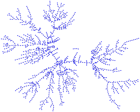
Figure 2. A random forest of size $n=1165$. It has two connected components.

Example 2.

A basic, but important example is that of forests, illustrated in Figure 2. We have in this case

$$C(z)=T(z)-\frac{T(z)^{2}}{2},$$

where $T(z)=ze^{T(z)}$ counts rooted trees (see for instance [19, p. 132]). The series $T$, $C$ and $A=e^{C}$ have radius of convergence $\rho=1/e$, with the following singular expansions at this point:

$$\begin{array}[]{lllllllllllcccccccccccccccccccc}T(z)=1&-\sqrt{2}({1-ze})^{{1/2}}&+\frac{2}{3}(1-ze)&-\frac{11\sqrt{2}}{36}(1-ze)^{{3/2}}&+O((1-ze)^{2}),\\ C(z)=\frac{1}{2}&&-(1-ze)&+\frac{2\sqrt{2}}{3}(1-ze)^{{3/2}}&+O((1-ze)^{2}),\\ A(z)=\sqrt{e}&&-\sqrt{e}(1-ze)&+\sqrt{e}\frac{2\sqrt{2}}{3}(1-ze)^{{3/2}}&+O((1-ze)^{2}).\end{array}$$ (6)

The singularity analysis of [19, Chap. VI] applies: the three series are analytic in a $\Delta$-domain, and their coefficients satisfy

$$t_{n}\sim n!\frac{e^{n}}{\sqrt{2\pi}n^{3/2}},\quad{c_{n}\sim n!\frac{e^{n}}{\sqrt{2\pi}n^{5/2}}},\quad\hbox{and}\quad{a_{n}\sim\sqrt{e}\,c_{n}}.$$

We will also consider rooted trees of height less than $k$ (where by convention the tree consisting of a single vertex has height $0$). Let $T_{k}(z)$ denote their generating function. Then $T_{1}(z)=z$ and for $k\geq 1$,

$$T_{k+1}(z)=ze^{T_{k}(z)}.$$

Note that $T_{k}(z)$ is entire.

Note. When all excluded minors are 2-connected, $C(\rho)$ always converges, but the nature of the singularity of $C(z)$ at $\rho$ depends on the class: it is for instance $(1-z/\rho)^{3/2}$ for forests (and more generally, for subcritical classes [14]), but $(1-z/\rho)^{5/2}$ for planar graphs. We refer to [20] for a more detailed discussion that applies to classes that exclude 3-connected minors.

Proposition 3 (Number of components — when excluded minors are 2-connected).

The mean of $N_{n}$ satisfies:

$$\mathbb{E}(N_{n})\sim 1+C(\rho)$$

and the random variable $N_{n}-1$ converges in law to a Poisson distribution of parameter $C(\rho)$. That is, as $n\rightarrow\infty$,

$$\mathbb{P}(N_{n}=i+1)\rightarrow\frac{C(\rho)^{i}}{i!e^{C(\rho)}}.$$ (7)

We refer to [26, Cor. 1.6] for a proof. The largest component is known to contain almost all vertices, and it is not hard to prove that the same holds for the root component. In fact, the tails of the random variables $S_{n}$ and $L_{n}$ are related by the following simple result.

Lemma 4.

For any class of graphs $\mathcal{A}$, and $k<n/2$,

$$\mathbb{P}(S_{n}=n-k)=\frac{n-k}{n}\,\mathbb{P}(L_{n}=n-k).$$

Proof.

Let us denote by $B_{n}$ the (lexicographically first) biggest component of $\mathcal{G}_{n}$. Its size is thus $L_{n}$. We have, for $n>2k$,

$$\mathbb{P}(S_{n}=n-k) = \mathbb{P}(S_{n}=n-k\hbox{ and }1\in B_{n})+\mathbb{P}(S_{n}=n-k\hbox{ and }1\not\in B_{n})$$

$$= \mathbb{P}(L_{n}=n-k\hbox{ and }1\in B_{n})+\mathbb{P}(S_{n}=n-k\hbox{ and }1\not\in B_{n})$$

$$= \mathbb{P}(1\in B_{n}|L_{n}=n-k)\mathbb{P}(L_{n}=n-k)+\mathbb{P}(S_{n}=n-k\hbox{ and }1\not\in B_{n})$$

$$= \frac{n-k}{n}\,\mathbb{P}(L_{n}=n-k).$$

Indeed, there cannot be two components of size $n-k$ or more. This implies that $\mathbb{P}(S_{n}=n-k\hbox{ and }1\not\in B_{n})=0$.  

Proposition 5 (The root component and the largest component — when excluded minors are 2-connected).

The random variables $n-S_{n}$ and $n-L_{n}$ both converge to a discrete limit distribution $X$ given by

$$\mathbb{P}(X=k)=\frac{1}{A(\rho)}\frac{a_{k}\rho^{k}}{k!}.$$

Proof.

By Lemma 4, the two statements are equivalent. The $L_{n}$ result has been proved by McDiarmid [26, Cor. 1.6].

We give an independent proof (of the $S_{n}$ result), as we will recycle its ingredients later for certain classes of graphs that avoid non-2-connected minors. Let $k\geq 0$ be fixed. By (2),

$$\mathbb{P}(S_{n}=n-k)=\frac{c_{n-k}a_{k}{n-1\choose k}}{a_{n}}=\frac{a_{k}}{k!}\ \frac{c_{n-k}}{a_{n-k}}\ \frac{(n-1)!a_{n-k}}{(n-k-1)!a_{n}}.$$

By Proposition 1, the term ${c_{n-k}}/{a_{n-k}}$, which is the probability that a graph of size $n-k$ is connected, converges to $1/A(\rho)$. Moreover, the sequence $a_{n}/n!$ is smooth, so that $\frac{(n-1)!a_{n-k}}{(n-k-1)!a_{n}}$ converges to $\rho^{k}$. The result follows.  

A more precise result is actually available. Let us call fragment the union of the components that differ from the biggest component $B_{n}$. Then McDiarmid describes the limit law of the fragment, not only of his size [26, Thm. 1.5]: the probability that the fragment is isomorphic to a given unlabelled graph $H$ of size $k$ is

$$\frac{1}{A(\rho)}\frac{\rho^{k}}{{\rm aut}(H)},$$

where ${\rm aut}(H)$ is the number of automorphisms of $H$.

4. When trees dominate: $\boldsymbol{C(z)}$ converges at $\boldsymbol{\rho}$

Let $\mathcal{A}$ be a decomposable class of graphs (for instance, a class defined by excluding connected minors), satisfying the following conditions:

1. $\mathcal{A}$ includes all trees,

2. the generating function $D(z)$ that counts the connected graphs of $\mathcal{A}$ that are not trees has radius of convergence (strictly) larger than $1/e$ (which is the radius of trees).

We then say that $\mathcal{A}$ is dominated by trees. Some examples are presented below. In this case, the properties that hold for forests (Section  3) still hold, except that the probability $c_{n}/a_{n}$ that $\mathcal{G}_{n}$ is connected tends to a limit that is now at most $1/\sqrt{e}$. We will see that this limit can become arbitrarily small.

Proposition 6 (The number of graphs — when trees dominate).

Let $T(z)$ be the generating function of rooted trees, given by $T(z)=ze^{T(z)}$. Write the generating function of connected graphs in the class $\mathcal{A}$ as

$$C(z)=T(z)-\frac{T(z)^{2}}{2}+D(z).$$

The generating function of graphs of $\mathcal{A}$ is $A(z)=e^{C(z)}.$ As $n\rightarrow\infty$,

$$c_{n}\sim n!\frac{e^{n}}{\sqrt{2\pi}n^{5/2}}\quad\hbox{and}\quad a_{n}\sim A(1/e)c_{n}.$$

In particular, the probability that $\mathcal{G}_{n}$ is connected tends to $1/A(1/e)=e^{-1/2-D(1/e)}$ as $n\rightarrow\infty$.

Proof.

As in Example 2, we use singularity analysis [19, Chap. VI]. By assumption, $D(z)$ has radius of convergence larger than $1/e$, and the singular behaviour of $C(z)$ is that of unrooted trees. More precisely, it follows from (6) that, as $z$ approaches $1/e$,

$$C(z)=1/2+D(1/e)-(1-ze)(1+D^{\prime}(1/e)/e)+\frac{2\sqrt{2}}{3}(1-ze)^{3/2}+O((1-ze)^{2}),$$

this expansion being valid in a $\Delta$-domain. This gives the estimate of $c_{n}$ via singularity analysis. For the series $A$, we find

$$A(z)=e^{1/2+D(1/e)}\left(1-(1-ze)(1+D^{\prime}(1/e)/e)+\frac{2\sqrt{2}}{3}(1-ze)^{3/2}+O((1-ze)^{2})\right),$$

and the estimate of $a_{n}$ follows.  

Proposition 7 (Number of components — when trees dominate).

The mean of $N_{n}$ satisfies:

$$\mathbb{E}(N_{n})\sim 1+C(1/e)$$

and $N_{n}-1$ converges in law to a Poisson distribution of parameter $C(1/e)$ (see (7)).

Proof.

We can start from (1) and apply singularity analysis. Or we can apply a ready-to-use result of Bell et al. [4, Thm. 2], which uses the facts (proved in Proposition 6) that the sequences $nc_{n-1}/c_{n}$ and $c_{n}/a_{n}$ converge.  

Proposition 8 (Size of components — when trees dominate).

The random variable $n-S_{n}$ converges to a discrete limit distribution $X$ given by

$$\mathbb{P}(X=k)=\frac{1}{A(1/e)}\frac{a_{k}e^{-k}}{k!},$$

where $a_{k}$ and $A(z)$ are given in Proposition 6. The same holds for $n-L_{n}$.

Proof.

The two ingredients used in the proof of Proposition 5 to establish the limit law of $n-S_{n}$ (namely, smoothness of $a_{n}/n!$ and convergence of $c_{n}/a_{n}$), still hold here (see Proposition 6). Lemma 4 gives then the law of $n-L_{n}$.  

We now present a collection of classes dominated by trees.

Proposition 9.

Let $k\geq 1$. Let $\mathcal{A}$ be a decomposable class of graphs that includes all trees, and such that all graphs of $\mathcal{A}$ avoid the $k$-spoon (shown in Figure 1). Then $\mathcal{A}$ is dominated by trees, and the results of Propositions 6, 7 and 8 hold.

Proof.

Clearly, it suffices to prove this proposition when $\mathcal{A}$ is exactly the class of graphs avoiding the $k$-spoon, which we henceforth assume.

We partition the set $\mathcal{C}$ of connected graphs of $\mathcal{A}$ into three subsets: the set $\mathcal{C}_{0}$ of trees, counted by $C_{0}=T-T^{2}/2$ with $T\equiv T(z)$, the set $\mathcal{C}_{1}$ of unicyclic graphs (counted by $C_{1}$), and finally the set $\mathcal{C}_{2}$ containing graphs with at least two cycles (counted by $C_{2}$). Hence $C=T-T^{2}/2+C_{1}+C_{2}$. We will prove that $C_{1}$ has radius of convergence (strictly) larger than $1/e$, and that $C_{2}$ is entire.

A unicyclic graph belongs to $\mathcal{C}$ if and only if all trees attached to its unique cycle have height less than $k$. The generating function of cycles is given by:

$$\operatorname{Cyc}(z)=\frac{1}{2}\sum_{n\geq 3}\frac{z^{n}}{n}=\frac{1}{2}\left(\log\frac{1}{1-z}-z-\frac{z^{2}}{2}\right).$$ (8)

Hence, the basic rules of the symbolic method of [19, Chap. II] give:

$$C_{1}(z)=\operatorname{Cyc}(T_{k})=\frac{1}{2}\left(\log\frac{1}{1-T_{k}(z)}-T_{k}(z)-\frac{T_{k}(z)^{2}}{2}\right),$$ (9)

where $T_{k}$ counts rooted trees of height less than $k$ and is given in Example 2. Recall from this example that $T(z)$ equals 1 at its unique dominant singularity $1/e$. Also, $T_{k}(z)<T(z)$ for all $z\in[0,1/e]$ since $T_{k}$ counts fewer trees than $T$. In particular, $T_{k}(1/e)<1$ and $C_{1}(z)$ has radius of convergence larger than $1/e$.

We now want to prove that $C_{2}$ is entire. The $(2)$-core of a connected graph $H$ is the (possibly empty) unique maximal subgraph of minimum degree 2. It can be obtained from $H$ by deleting recursively all vertices of degree 0 or 1 (or, in a non-recursive fashion, all dangling trees of $H$). By extension, we call core any connected graph of minimum degree 2. Let $\bar{\mathcal{C}}_{2}$ denote the set of cores having several cycles and avoiding the $k$-spoon, and $\bar{C}_{2}$ the associated generating function. The inequality

$$C_{2}(z)\leq\bar{C}_{2}(T_{k}(z))$$

holds, coefficient by coefficient, because the core of a graph of $\mathcal{C}_{2}$ has several cycles and avoids the $k$-spoon. Since $T_{k}$ is entire, it suffices to prove that $\bar{C}_{2}$ is entire. It follows from [6, Thm. 3.1] that it suffices to prove that no graph $G$ of $\bar{\mathcal{C}}_{2}$ contains a path of length $3k-1$. So let $P=(v_{0},v_{1},\ldots,v_{\ell})$ be a path of maximal length in $G$, and assume that $\ell\geq 3k-1$. We will prove that $G$ contains the $k$-spoon as a minor. Since $P$ is maximal and $G$ is a core, there exist $v_{i}$ and $v_{j}$, with $i\geq 2$ and $j\leq\ell-2$, such that the edges $\{v_{0},v_{i}\}$ and $\{v_{j},v_{\ell}\}$ belong to $G$.

If $i=\ell$ or $j=0$, let $\bar{P}$ be the cycle of $G$ formed of $P$ and the edge $\{v_{0},v_{\ell}\}$. Let $\bar{Q}$ be another cycle of $G$. If $\bar{Q}$ contains at most one vertex of $P$ (Figure 3(a)), we find an $\ell$-spoon by deleting one edge of $\bar{P}$, contracting $\bar{Q}$ into a 3-cycle and one of the paths joining $P$ to $\bar{Q}$ into a point. If $\bar{Q}$ contains at least two vertices $v_{a}$ and $v_{b}$ of $P$, with $a<b$ (Figure 3(b)), we may assume that $\bar{Q}$ consists of the edges $\{v_{a},v_{a+1}\},\ldots,\{v_{b-1},v_{b}\}$ and of a path $Q$ that only meets $P$ at $v_{a}$ and $v_{b}$. Let $\bar{R}$ denote the cycle formed of the path $Q$ and the path $(v_{b},v_{b+1},\ldots,v_{\ell},v_{0},\ldots,v_{a}\}$. Then we obtain a $p$-spoon, with $p\geq\lceil 3k/2\rceil-1\geq k$, by contracting the shortest of the cycles $\bar{Q}$ and $\bar{R}$ into a 3-cycle and deleting an edge ending at $v_{a}$ from the other.

Figure 3. A core having several cycles and avoiding the $k$-spoon cannot contain a path of length $3k-1$.

Assume now that $i<\ell$ and $j>0$. Suppose first that $i\leq j$ (Figure 3(c)). By symmetry, we may assume that the cycle $\bar{P}_{1}=(v_{0},\ldots,v_{i})$ is shorter than (or equal in length to) the cycle $\bar{P}_{2}=(v_{j},\ldots,v_{\ell})$. In particular, $i\leq\ell/2$. Contract $\bar{P}_{1}$ into a 3-cycle, and remove the edge $\{v_{j},v_{\ell}\}$ from $\bar{P}_{2}$: this gives a $p$-spoon with $p=\ell-i\geq\lceil\ell/2\rceil\geq k$. Assume now that $j<i$ (Figure 3(d)). Consider the three following paths joining $v_{i}$ and $v_{j}$: $(v_{i},v_{i-1},\ldots,v_{j})$, $(v_{i},v_{0},v_{1},\ldots,v_{j})$ and $(v_{i},v_{i+1},\ldots,v_{\ell},v_{j})$. Since the sum of the lengths of these paths is $\ell+2\geq 3k+1$, one of them, say $(v_{i},v_{0},v_{1},\ldots,v_{j})$, has length at least $k+1$. That is, $j\geq k$. Delete from this path the edge $\{v_{i},v_{0}\}$, and contract the cycle formed by the other two paths into a 3-cycle: this gives a $j$-spoon, with $j\geq k$.  

The simplest non-trivial class of graphs satisfying the conditions of Proposition 9 consists of graphs avoiding the 1-spoon. By specializing to $k=1$ the proof of that proposition, we find $C_{1}=\operatorname{Cyc}(z)$ and $C_{2}=0$ (since no core having several cycles avoids the 2-path). Hence

$$C(z)=T(z)-\frac{T(z)^{2}}{2}+\frac{1}{2}\left(\log\frac{1}{1-z}-z-\frac{z^{2}}{2}\right).$$

More generally, consider the class $\mathcal{A}^{(k)}$ of graphs avoiding the $k$-spoon, but also the diamond and the bowtie (both shown in Figure 1): excluding the latter two graphs means that no graph of $\mathcal{C}$ can have several cycles, so that $C_{2}=0$. Hence the proof of Proposition 9 immediately gives the following result.

Figure 4. A random graph of size $n=541$ avoiding the diamond, the bowtie and the 20-spoon.

Proposition 10 (No diamond, bowtie or $k$-spoon).

Let $k\geq 1$. Let $T(z)$ be the generating function of rooted trees, given by $T(z)=ze^{T(z)}$, and let $T_{k}(z)$ be the generating function of rooted trees of height less than $k$, given in Example 2.

Let $\mathcal{A}^{(k)}$ be the class of graphs avoiding the diamond, the bowtie and the $k$-spoon. The generating function of connected graphs of $\mathcal{A}^{(k)}$ is

$$C^{(k)}(z)=T(z)-\frac{T(z)^{2}}{2}+D^{(k)}(z)$$

where

$$D^{(k)}(z)=\frac{1}{2}\left(\log\frac{1}{1-T_{k}(z)}-T_{k}(z)-\frac{T_{k}(z)^{2}}{2}\right).$$

The class $\mathcal{A}^{(k)}$ is dominated by trees, and the results of Propositions 6, 7 and 8 hold. In particular, the probability that a random graph of $\mathcal{A}_{n}^{(k)}$ is connected tends to $e^{-C^{(k)}(1/e)}$ as $n\rightarrow\infty$. Since $T_{k}(1/e)$ tends to $T(1/e)=1$ as $k$ increases, this limit probability tends to $0$.

A random graph of $\mathcal{A}_{n}^{(k)}$ is shown in Figure 4 for $k=20$ and $n=541$. We have also determined the generating function of graphs that avoid the 2-spoon.

Proposition 11 (No 2-spoon).

Let $T(z)$ be the generating function of rooted trees, given by $T(z)=ze^{T(z)}$. The generating function of connected graphs avoiding the $2$-spoon is

$$C(z)=T(z)-\frac{T(z)^{2}}{2}+D(z)$$

where

$$D(z)=\frac{1}{2}\left(\log\frac{1}{1-ze^{z}}-ze^{z}-\frac{z^{2}e^{2z}}{2}\right)+\frac{z^{4}}{4!}+z^{2}e^{2z}\left(e^{z}-1-z-\frac{z^{2}}{4}\right).$$

The class of graphs avoiding the $2$-spoon is dominated by trees, and the results of Propositions 6, 7 and 8 apply.

Proof.

We first follow the proof of Proposition 9: we write $C=T-T^{2}/2+C_{1}+C_{2}$, where $C_{1}$ is given by (9) with $T_{k}=T_{2}=ze^{z}$, and $C_{2}$ counts connected graphs having several cycles and avoiding the $2$-spoon. Note that $C_{1}$ is the first term in the above expression of $D(z)$. Let us now focus on $C_{2}$.

In Section 10 below, we study the class of graphs that avoid the bowtie, and in particular describe the cores of this class (Proposition 31). Since the bowtie contains the 2-spoon as a minor, graphs that avoid the 2-spoon avoid the bowtie as well. Hence we will first determine which cores of Proposition 31 have several cycles and avoid the 2-spoon, and then check which of their vertices can be replaced by a small tree (that is, a tree of height 1) without creating a 2-spoon.

Clearly, the cores of Proposition 31 that have several cycles are those of Figures 16, 17 and 18. Among the cores of Figure 16, only $K_{4}$ avoids the 2-spoon. Moreover, none of its vertices can be replaced by a non-trivial tree. This gives the term $z^{4}/4!$ in $D(z)$. Among the cores of Figures 17 and 18, only the ones drawn on the left-hand sides avoid the 2-spoon. In these cores, only the two vertices of degree at least 3 can be replaced by a small tree. The resulting graphs are shown in Figure 5 and give together the contribution

$$\frac{1}{2}(ze^{z})^{2}\left(e^{z}-1-z\right)+\frac{1}{2}(ze^{z})^{2}\left(e^{z}-1-z-\frac{z^{2}}{2}\right)$$

(again an application of the symbolic method of [19, Chap. II]). The proposition follows.  

Figure 5. Graphs with several cycles avoiding the $2$-spoon.

5. Excluding the diamond and the bowtie: a logarithmic singularity

Figure 6. A random graph of size $n=859$ avoiding the diamond and the bowtie.

Let $\mathcal{A}$ be the class of graphs avoiding the diamond and the bowtie (both shown in Figure 1). These are the graphs whose components have at most one cycle (Figure 6). They were studied a long time ago by Rényi [31] and Wright [34], and the following result has now become a routine exercise.

Proposition 12 (The number of graphs avoiding a diamond and a bowtie).

Let $T(z)$ be the generating function of rooted trees, defined by $T(z)=ze^{T(z)}$. The generating function of connected graphs of $\mathcal{A}$ is

$$C(z)=\frac{T(z)}{2}-\frac{3T(z)^{2}}{4}+\frac{1}{2}\log\frac{1}{1-T(z)}.$$

The generating function of graphs of $\mathcal{A}$ is $A(z)=e^{C(z)}.$ As $n\rightarrow\infty$,

$$c_{n}\sim n!\frac{e^{n}}{4n}\quad\hbox{and}\quad a_{n}\sim n!\,\frac{1}{(2e)^{1/4}\Gamma(1/4)}\frac{e^{n}}{n^{3/4}}.$$ (10)

In particular, the probability that $\mathcal{G}_{n}$ is connected tends to $0$ at speed $n^{-1/4}$ as $n\rightarrow\infty$.

Proof.

The expression of $C(z)$ is obtained by taking the limit $k\rightarrow\infty$ in Proposition 10.

We now estimate $c_{n}$ and $a_{n}$ via singularity analysis [19, Sect. VI.4]. Recall from Example 2 that $T(z)$ has a unique dominant singularity, at $z=1/e$, with a singular expansion (6) valid in a $\Delta$-domain. Thus $1/e$ is also the unique dominant singularity of $C(z)$ and $A(z)$, and we have, in a $\Delta$-domain,

$$C(z)\sim\frac{1}{4}\log\left(\frac{1}{1-ze}\right)\quad\hbox{and}\quad A(z)\sim\frac{1}{(2e)^{1/4}(1-ez)^{1/4}}.$$ (11)

The asymptotic estimates of $c_{n}$ and $a_{n}$ follow.  

Proposition 13 (Number of components — no bowtie nor diamond).

The mean and variance of $N_{n}$ satisfy:

$$\mathbb{E}(N_{n})\sim\frac{\log n}{4},\quad\quad\mathbb{V}(N_{n})\sim\frac{\log n}{4},$$

and the random variable $\frac{N_{n}-\log n/4}{\sqrt{\log n/4}}$ converges in law to a standard normal distribution.

Proof.

Using (6), the estimate (11) can be refined into

$$C(z)=\frac{1}{4}\log\left(\frac{1}{1-ze}\right)+\lambda+O(\sqrt{1-ze}),$$ (12)

where $\lambda$ is a constant, and the proposition is a direct application of [19, Prop. IX.14, p. 670].  

The number of connected components is about $1/4\log n$. However, the size of the root component is found to be of order $n$. More precisely, we have the following result.

Proposition 14 (Size of the root component — no bowtie nor diamond).

The normalized variable $S_{n}/n$ converges in distribution to a beta law of parameters $\alpha=1,\beta=1/4$, with density $(1-x)^{-3/4}/4$ on $[0,1]$. In fact, a local limit law holds: for $x\in(0,1)$ and $k=\lfloor xn\rfloor$,

$$n\,\mathbb{P}(S_{n}=k)\rightarrow\frac{1}{4}(1-x)^{-3/4}.$$

The convergence of moments holds as well: for $i\geq 0$,

$$\mathbb{E}(S_{n}^{i})\sim\frac{\Gamma(5/4)i!}{\Gamma(i+5/4)}n^{i}.$$

Proof.

Recall that the existence of a local limit law implies the existence of a global one [9, Thm. 3.3]. Thus it suffices to prove the local limit law. But this is easy, starting from the rightmost expression in (2), and using (10).

For the moments, let us start from (4). Our first task is to obtain an estimate of $C^{(i+1)}(z)$ near $1/e$. Combining (12) and [19, Thm. VI.8, p. 419] gives, for $i\geq 1$,

$$C^{(i+1)}(z)\sim\frac{i!}{4}\left(\frac{e}{{1-ze}}\right)^{i+1}.$$

We multiply this by the estimate (11) of $A(z)$, apply singularity analysis, and finally use (10) to obtain the asymptotic behaviour of the $i$th moment of $S_{n}$. Since these moments characterize the above beta distribution, we conclude [19, Thm. C.2] that $S_{n}/n$ converges in law to this distribution.  

Figure 7. The distribution function $\mathbb{P}(L_{n}<m)$ for $n=100$. The first plot shows the change of regime at $m=n/2$, the second the change at $m=n/3$, the third the change at $m=n/4$.

We conclude with the law of the size of the largest component, which we derive from general results dealing with components of logarithmic structures [2]. The following proposition is illustrated by Figure 7.

Proposition 15 (Size of the largest component — no bowtie nor diamond).

The normalized variable $L_{n}/n$ converges in law to the first component of a Poisson-Dirichlet distribution of parameter $1/4$: for $x\in(0,1)$,

$$\mathbb{P}(L_{n}<xn)\rightarrow\rho(1/x),$$

where $\rho:{\mathbb{R}}^{+}\rightarrow[0,1]$ is the unique continuous function such that $\rho(x)=1$ for $x\in[0,1]$ and for $x>1$,

$$x^{1/4}\rho^{\prime}(x)+\frac{1}{4}(x-1)^{-3/4}\rho(x-1)=0.$$

The function $\rho$ is infinitely differentiable, except at integer points.

A local limit law also holds: for $x\in(0,1)$ and $1/x\not\in{\mathbb{N}}$,

$$n\,\mathbb{P}(L_{n}=\lfloor xn\rfloor)\rightarrow\frac{(1-x)^{-3/4}}{4x}\,\rho\left(\frac{1-x}{x}\right).$$

Proof.

A decomposable class of graphs $\mathcal{A}$ is an assembly in the sense of [2, Sec. 2.2]. In particular, it satisfies the conditioning relation [2, Eq. (3.1)]: conditionally to the total size being $n$, the numbers $C_{i}^{(n)}$ that count connected components of size $i$, for $1\leq i\leq n$, are independent. When $\mathcal{A}$ is the class of graphs avoiding the diamond and the bowtie, the estimate (10) of $c_{n}$ tells us that this assembly is logarithmic in the sense of [2, Eq. (2.15)]: indeed, [2, Eq. (2.16)] holds with $m_{i}=c_{i}$, $y=e$ and $\theta=1/4$. Our random variable $L_{n}$ coincides with the random variable $L_{1}^{(n)}$ of [2]. We then apply Theorem 6.12 and Theorem 6.8 of [2]: this gives the convergence in law of $L_{n}$ and the local limit law. The distribution function of the limit law is given by [2, Eq. (5.29)], and the differential equation satisfied by $\rho$ follows from [2, Eq. (4.23)].  

Remark. If we push further the singular expansion (12) of $C(z)$, we find a subdominant term in $\sqrt{1-ze}$, but its influence is never felt in the asymptotics results. We would obtain the same results (with possibly different constants) for any $C(z)$ having a purely logarithmic singularity.

6. Hayman admissibility and extensions

Our next examples (Sections 7 to 10) deal with examples where $C(z)$ diverges at $\rho$ with an algebraic singularity. This results in $A(z)$ diverging rapidly at $\rho$. We then estimate $a_{n}$ using the saddle point method — more precisely, with a black box that applies to Hayman-admissible (or H-admissible) functions. Let us first recall what this black box does [19, Thm. VIII.4, p. 565].

Theorem 16.

Let $A(z)$ be a power series with real coefficients and radius of convergence $\rho\in(0,\infty]$. Assume that $A(r)$ is positive for $r\in(R,\rho)$, for some $R\in(0,\rho)$. Let

$$a(r)=r\frac{A^{\prime}(r)}{A(r)}\quad\hbox{and}\quad b(r)=r\frac{A^{\prime}(r)}{A(r)}+r^{2}\frac{A^{\prime\prime}(r)}{A(r)}-r^{2}\left(\frac{A^{\prime}(r)}{A(r)}\right)^{2}.$$

Assume that the following three properties hold:

1. [Capture condition]

   $$\lim_{r\rightarrow\rho}a(r)=\lim_{r\rightarrow\rho}b(r)=+\infty.$$

2. [Locality condition] For some function $\theta_{0}(r)$ defined over $(R,\rho)$, and satisfying $0<\theta_{0}(r)<\pi$, one has, as $r\rightarrow\rho$,

   $$\sup_{|\theta|\leq\theta_{0}(r)}\left|\frac{A(re^{i\theta})}{A(r)}e^{-i\theta a(r)+\theta^{2}b(r)/2}-1\right|\rightarrow 0.$$

3. [Decay condition] As $r\rightarrow\rho$,

   $$\sup_{|\theta|\in[\theta_{0}(r),\pi)}\left|\frac{A(re^{i\theta})}{A(r)}{\sqrt{b(r)}}\right|\rightarrow 0.$$

We say that $A(z)$ is Hayman admissible. Then the $n$th coefficient of $A(z)$ satisfies, as $n\rightarrow\infty$,

$$[z^{n}]A(z)\sim\frac{A(\zeta)}{\zeta^{n}\sqrt{2\pi b(\zeta)}}$$ (13)

where $\zeta\equiv\zeta_{n}$ is the unique solution in $(R,\rho)$ of the saddle point equation $\zeta A^{\prime}(\zeta)=nA(\zeta).$

Conditions $\bf H_{2}$ and $\bf H_{3}$ are usually stated in terms of uniform equivalence as $r\rightarrow\rho$, but we find the above formulation more explicit.

The set of H-admissible series has several useful closure properties [19, Thm. VIII.5, p. 568]. Here is one that we were not able to find in the literature.

Theorem 17.

Let $A(z)=F(z)G(z)$ where $F(z)$ and $G(z)$ are power series with real coefficients and radii of convergence $0<\rho_{F}<\rho_{G}\leq\infty$. Assume that $F(z)$ has non-negative coefficients and is Hayman-admissible, and that $G(\rho_{F})>0$. Then $A(z)$ is Hayman-admissible.

Proof.

Let us first prove that the radius of convergence $\rho$ of $A(z)$ is $\rho_{F}$. Clearly, $\rho\geq\rho_{F}$. Now, suppose $\rho>\rho_{F}$. Then $A(z)$ is analytic at $\rho_{F}$. Together with $G(\rho_{F})>0$ this implies that $F(z)=A(z)/G(z)$ has an analytic continuation at $\rho_{F}$, which is impossible by Pringsheim’s Theorem (since $F(z)$ has non-negative coefficients) [19, Thm. IV.6, p. 240]. Note also that $A(r)$ is positive on an interval of the form $[R,\rho)$ (by continuity of $G$). Let us now check the three conditions of Theorem 16. We have

$$a(r)=a_{F}(r)+a_{G}(r),\quad\quad b(r)=b_{F}(r)+b_{G}(r),$$

with

$$a_{F}(r)=r\frac{F^{\prime}(r)}{F(r)}\quad\hbox{and}\quad b_{F}(r)=r\frac{F^{\prime}(r)}{F(r)}+r^{2}\frac{F^{\prime\prime}(r)}{F(r)}-r^{2}\left(\frac{F^{\prime}(r)}{F(r)}\right)^{2},$$

and similarly for $a_{G}$ and $b_{G}$.

$\bf H_{1}$ The capture condition holds for $A$ since it holds for $F$, given that $G(\rho)>0$ and $\rho_{G}>\rho$.

$\bf H_{2}$ Choose $\theta_{0}(r)=\theta_{0}^{F}(r)$ where $\theta_{0}^{F}(r)$ is a function for which $F(z)$ satisfies $\bf H_{2}$ and $\bf H_{3}$. We have

$$\frac{A(re^{i\theta})}{A(r)}\cdot e^{-ia(r)\theta+\theta^{2}b(r)/2}=\frac{F(re^{i\theta})}{F(r)}e^{-ia_{F}(r)\theta+\theta^{2}{b_{F}(r)}/2}\frac{G(re^{i\theta})}{G(r)}\cdot e^{-ia_{G}(r)\theta+\theta^{2}{b_{G}^{2}(r)}/{2}}.$$ (14)

By assumption, $F$ satisfies the locality condition: hence

$$\frac{F(re^{i\theta})}{F(r)}\cdot e^{-ia_{F}(r)\theta+{b_{F}(r)\theta^{2}}/{2}}=1+M(r,\theta)$$ (15)

where

$$\sup_{|\theta|\leq\theta_{0}(r)}\left|M(r,\theta)\right|\rightarrow 0$$ (16)

as $r\rightarrow\rho$. For $r\in[R,\rho)$ and $|\theta|\leq\theta_{0}(r)$, let us expand $\log G(re^{i\theta})$ in powers of $\theta$:

$$\log G(re^{i\theta})=\log G(r)+i\theta a_{G}(r)-\frac{\theta^{2}}{2}b_{G}(r)+{\theta^{3}}S(r,\theta)$$

where $S(r,\theta)$ is bounded uniformly in a neighborhood of $(\rho,0)$. We can assume that $\theta_{0}(r)\rightarrow 0$ as $r\rightarrow\rho$ (see [22, Eq. (12.1)]). Thus

$$\frac{G(re^{i\theta})}{G(r)}\cdot e^{-ia_{G}(r)\theta+\theta^{2}{b_{G}(r)}/{2}}=e^{\theta^{3}S(r,\theta)}=1+N(r,\theta)$$ (17)

where

$$\sup_{|\theta|\leq\theta_{0}(r)}\left|N(r,\theta)\right|\rightarrow 0$$ (18)

as $r\rightarrow\rho$. Putting together Eqs. (14) to (18), we obtain that $A(z)$ satisfies $\bf H_{2}$.

$\bf H_{3}$ We have:

$$\left|\frac{A(re^{i\theta})}{A(r)}\sqrt{b(r)}\right| = \left|\frac{F(re^{i\theta})G(re^{i\theta})}{F(r)G(r)}\sqrt{b_{F}(r)+b_{G}(r)}\right|$$

$$\leq \left|\frac{F(re^{i\theta})}{F(r)}\sqrt{2b_{F}(r)}\cdot\frac{G(re^{i\theta})}{G(r)}\right|\hskip 56.9055pt\hbox{for }r\hbox{ close to }\rho,$$

because $b_{F}(r)\rightarrow\infty$ as $r\rightarrow\rho$ while $b_{G}(r)$ is bounded around $\rho$. Also, since $G$ has radius larger than $\rho$ and $G(\rho)>0$, the term $G(re^{i\theta})/G(r)$ is uniformly bounded in a neighborhood of the circle of radius $\rho$. Since by assumption, $F(z)$ satisfies $\bf H_{3}$, this shows that $A(z)$ satisfies it as well.  

We will also need a uniform version of Hayman-admissibility for series of the form $e^{uC(z)}$.

Theorem 18.

Let $C(z)$ be a power series with non-negative coefficients and radius of convergence $\rho$. Assume that $A(z)=e^{C(z)}$ has radius $\rho$ and is Hayman-admissible. Define

$$b(r)=rC^{\prime}(r)+r^{2}C^{\prime\prime}(r)\quad\hbox{and}\quad V(r)=C(r)-\frac{(rC^{\prime}(r))^{2}}{rC^{\prime}(r)+r^{2}C^{\prime\prime}(r)}.$$

Assume that, as $r\rightarrow\rho$,

$$V(r) \rightarrow +\infty,$$ (19)

$$\frac{C(r)}{V(r)^{3/2}} \rightarrow 0,$$ (20)

$$b(r)^{1/\sqrt{V(r)}} = O(1).$$ (21)

Then $A(z,u):=e^{uC(z)}$ satisfies Conditions (1)–(6), (8) and (9) of [16, Def. 1]. If $N_{n}$ is a sequence of random variables such that

$$\mathbb{P}(N_{n}=i)=\frac{[z^{n}]C(z)^{i}}{i![z^{n}]e^{C(z)}},$$

then the mean and variance of $N_{n}$ satisfy:

$$\mathbb{E}(N_{n})\sim C(\zeta_{n}),\quad\quad\mathbb{V}(N_{n})\sim V(\zeta_{n}),$$ (22)

where $\zeta_{n}\equiv\zeta$ is the unique solution in $(0,\rho)$ of the saddle point equation $\zeta C^{\prime}(\zeta)=n$. Moreover, the normalized version of $N_{n}$ converges in law to a standard normal distribution:

$$\frac{N_{n}-\mathbb{E}(N_{n})}{\sqrt{\mathbb{V}(N_{n})}}\rightarrow\mathcal{N}(0,1).$$

Remark. The set of series covered by this theorem seem to have only a small intersection with the set of series (of the form $g(z)F(uf(z))$) covered by Section 4 of [17].

Proof.

With the notation of [16, Def. 1], we have

$$\begin{array}[]{lll}a(r,u)=c(r,u)=ruC^{\prime}(r)=ua(r),&&b(r,u)=ruC^{\prime}(r)+r^{2}uC^{\prime\prime}(r)=ub(r),\\ \\ \bar{a}(r,u)=\bar{b}(r,u)=uC(r),&&\varepsilon(r)=\displaystyle\frac{K}{\sqrt{V(r)}}\end{array}$$ (23)

for a fixed constant $K$. Condition (1) of [16, Def. 1] holds for $R=\rho$, any $\zeta>0$ and any $R_{0}\in[0,\rho)$: indeed, the series $A(z,u)$ is analytic for $|z|<\rho$ and $u\in{\mathbb{C}}$, and $A(z,1)$ is positive on $[0,\rho)$. Conditions (8) and (9) are nothing but our assumptions (19) and (20). Condition (4) is that $b(r)\rightarrow+\infty$ as $r\rightarrow\rho$: this holds because $A$ is Hayman admissible. Condition (5) requires that $b(r,u)\sim b(r,1)$ for $r\rightarrow\rho$, uniformly for $u\in[1-\varepsilon(r),1+\varepsilon(r)]$: this holds because $b(r,u)/b(r,1)=u$ and $\varepsilon(r)\rightarrow 0$ as $r\rightarrow\rho$. Condition (6) requires that $a(r,u)=a(r,1)+c(r,1)(u-1)+O(c(r,1)(u-1)^{2}))$ uniformly for $r\in(0,\rho)$ and $u\in[1-\varepsilon(r),1+\varepsilon(r)]$. Since $a(r,u)=a(r,1)+c(r,1)(u-1)$, this condition obviously holds.

We are thus left with Conditions (2) and (3), which are uniform versions (in $u$) of the locality and decay conditions $\bf H_{2}$ and $\bf H_{3}$ defining Hayman admissibility. They can be stated as follows.

1. [Uniform locality condition] There exists $R\in(0,\rho)$ such that for any $K>0$, there exists a function $\delta(r)$ defined over $(R,\rho)$, and satisfying $0<\delta(r)<\pi$, such that, as $r\rightarrow\rho$,

   $$\sup_{\large{|\theta|\leq\delta(r),\atop|u-1|\leq\varepsilon(r)}}\left|\frac{A(re^{i\theta},u)}{A(r,u)}e^{-i\theta a(r,u)+\theta^{2}b(r,u)/2}-1\right|\rightarrow 0.$$

2. [Uniform decay condition] As $r\rightarrow\rho$,

   $$\sup_{|\theta|\in[\delta(r),\pi)\atop|u-1|\leq\varepsilon(r)}\left|\frac{A(re^{i\theta},u)}{A(r,u)}{\sqrt{b(r,u)}}\right|\rightarrow 0.$$

We begin with $\bf H_{2}^{\prime}$. Since $A(z)$ is H-admissible, let $\theta_{0}(r)$ be a function for which $\bf H_{2}$ (and $\bf H_{3}$) holds:

$$\frac{A(re^{i\theta})}{A(r)}e^{-i\theta a(r)+\theta^{2}b(r)/2}=1+M(r,\theta)$$

where

$$M(r):=\sup_{|\theta|\leq\theta_{0}(r)}|M(r,\theta)|$$

tends to 0 as $r\rightarrow\rho$. Then, for $u\in[1-\varepsilon(r),1+\varepsilon(r)]$,

$$\frac{A(re^{i\theta},u)}{A(r,u)}e^{-i\theta a(r,u)+\theta^{2}b(r,u)/2} = \exp\left(u\left(C(re^{i\theta})-C(r)-i\theta a(r)+\theta^{2}b(r)/2\right)\right)$$

$$= (1+M(r,\theta))^{u}$$

where we have taken the principal determination of $\log$ to define $(1+M(r,\theta))^{u}=\exp(u\log(1+M(r,\theta)))$ (because $M(r,\theta)$ is close to $0$). Thus

$$\sup_{|\theta|\leq\theta_{0}(r)\atop|u-1|\leq\varepsilon(r)}\left|\frac{A(re^{i\theta},u)}{A(r,u)}e^{-i\theta a(r,u)+\theta^{2}b(r,u)/2}-1\right| = \sup_{|\theta|\leq\theta_{0}(r)\atop|u-1|\leq\varepsilon(r)}\left|(1+M(r,\theta))^{u}-1\right|$$

$$\leq (1+\varepsilon(r))M(r)+O\left((1+\varepsilon(r))M(r)^{2}\right),$$

and this upper bound tends to 0 as $r\rightarrow\rho$. This proves $\bf H_{2}^{\prime}$ with $\delta(r)=\theta_{0}(r)$.

We finally address $\bf H_{3}^{\prime}$. Since $A(z)$ satisfies the decay condition $\bf H_{3}$, the quantity

$$N(r,\theta):=\frac{A(re^{i\theta})}{A(r)}\sqrt{b(r)}\$$

satisfies

$$\sup_{|\theta|\in[\theta_{0}(r),\pi]}\left|N(r,\theta)\right|\rightarrow 0$$ (24)

as $r\rightarrow\rho$. We have, for $u\in[1-\varepsilon(r),1+\varepsilon(r)]$,

$$\left|\frac{A(re^{i\theta},u)}{A(r,u)}\sqrt{b(r,u)}\right| = \left|N(r,\theta)\right|^{u}{\sqrt{b(r)}^{1-u}}{\sqrt{u}}$$

$$\leq \left|N(r,\theta)\right|^{1+\varepsilon(r)}{\sqrt{b(r)}^{\varepsilon(r)}}{\sqrt{1+\varepsilon(r)}},$$

and this tends to $0$ uniformly for $|\theta|\in[\theta_{0}(r),\pi]$ thanks to (24), (23), (19) and (21).

As explained in [16] just below Theorem 2, these eight conditions give the estimates (22) of $\mathbb{E}(N_{n})$ and $\mathbb{V}(N_{n})$ and imply the existence of a gaussian limit law.  

We finish this section with a simple but useful result of products of series [5, Thm. 2].

Proposition 19.

Let $F(z)=\sum_{n}f_{n}{z^{n}}$ and $G(z)=\sum_{n}g_{n}{z^{n}}$ be power series with radii of convergence $0\leq\rho_{F}<\rho_{G}\leq\infty$, respectively. Suppose that $G(\rho_{F})\not=0$ and the sequence $(f_{n})_{n\geq 0}$ is smooth. Then $[z^{n}]F(z)G(z)\sim G(\rho_{F})f_{n}$.

7. Graphs with bounded components: $\boldsymbol{C(z)}$ is a polynomial

Let $\mathcal{C}$ be a finite class of connected graphs, and let $\mathcal{A}$ be the class of graphs with connected components in $\mathcal{C}$. Note that $\mathcal{A}$ is minor-closed if and only if $\mathcal{C}$ itself is minor-closed. This is the case for instance if $\mathcal{C}$ is the class of graphs of size at most $k$. In general, we denote by $k$ the size of the largest graphs of $\mathcal{C}$. We assume that $C(z)$ is aperiodic.

We begin with the enumeration of the graphs of $\mathcal{A}$. The following proposition is a bit more precise than the standard result on exponentials of polynomials [19, Cor. VIII.2, p. 568], since it makes explicit the behaviour of the term $b(\zeta)$ occurring in the saddle point estimate (13).

Proposition 20 (The number of graphs with small components).

Write the generating function of graphs of $\mathcal{C}$ as

$$C(z)=\sum_{i=0}^{k}\frac{c_{i}}{i!}z^{i}.$$ (25)

The generating function of graphs of $\mathcal{A}$ is $A(z)=e^{C(z)}.$ As $n\rightarrow\infty$,

$$a_{n}\sim n!\,\frac{1}{\sqrt{2\pi kn}}\frac{A(\zeta)}{\zeta^{n}}$$ (26)

where $\zeta\equiv\zeta_{n}$ is defined by $\zeta C^{{}^{\prime}}(\zeta)=n$ and satisfies

$$\zeta=\alpha n^{1/k}+\beta+O(n^{-1/k})$$ (27)

with

$$\alpha=\left(\frac{(k-1)!}{c_{k}}\right)^{1/k}\quad\hbox{and }\quad\beta=-\frac{(k-1)c_{k-1}}{kc_{k}}.$$ (28)

The probability that $\mathcal{G}_{n}$ is connected is of course zero as soon as $n>k$.

Proof.

The series $A(z)$ is H-admissible ([19, Thm. VIII.5, p. 568]) and Theorem 16 applies. The saddle point equation $\zeta C^{\prime}(\zeta)=n$ is an irreducible bivariate polynomial in $\zeta$ and $n$, of degree $k$ in $\zeta$. Consider $1/n$ as a small parameter $x$. By [33, Prop. 6.1.6], the saddle point $\zeta$ admits an expansion of the form

$$\zeta=\sum_{i\geq i_{0}}\alpha_{i}n^{-i/k},$$ (29)

for some integer $i_{0}$ and complex coefficients $\alpha_{i}$. Using Newton’s polygon method [19, p. 499], one easily finds $i_{0}=-1$ and the values (28) of the first two coefficients.

Since $b(r)=rC^{\prime}(r)+r^{2}C^{\prime\prime}(r)$ has leading term $kc_{k}r^{k}/(k-1)!$, the first order expansion of $b(\zeta)$ reads

$$b(\zeta)=kn+O(n^{(k-1)/k}),$$

and the asymptotic behaviour of $a_{n}$ follows.  

Again, the following proposition is more precise than the statement found, for instance, in [11, Thm. I], because our estimates of $\mathbb{E}(N_{n})$ and $\mathbb{V}(N_{n})$ are explicit. Note in particular that $\mathbb{E}(N_{n})\sim n/k$ suggests that most components have maximal size $k$.

Proposition 21 (Number of components — Graphs with small components).

Assume that the coefficient $c_{k-1}$ in (25) is non-zero. The mean and variance of $N_{n}$ satisfy:

$$\mathbb{E}(N_{n})\sim\frac{n}{k},\quad\quad\mathbb{V}(N_{n})\sim\frac{c_{k-1}}{k\cdot k!}\alpha^{k-1}n^{(k-1)/k},$$

where $\alpha$ is given by (28), and the random variable $\frac{N_{n}-\mathbb{E}(N_{n})}{\sqrt{\mathbb{V}(N_{n})}}$ converges in law to a standard normal distribution.

Proof.

We apply [11, Thm. I] (we can also apply Theorem 18 if $k>3$). Still denoting the saddle point by $\zeta\equiv\zeta_{n}$, we just have to find estimates of

$$\mu_{n}=C(\zeta)\quad\hbox{ and }\quad\sigma_{n}^{2}=C(\zeta)-\frac{(\zeta C^{\prime}(\zeta))^{2}}{\zeta C^{\prime}(\zeta)+\zeta^{2}C^{\prime\prime}(\zeta)}.$$

Given (27), we obtain

$$\mu_{n}=\frac{n}{k}+\frac{c_{k-1}}{k!}\alpha^{k-1}n^{(k-1)/k}+O(n^{(k-2)/k}),$$

$$\zeta^{2}C^{\prime\prime}(\zeta)=(k-1)n-\frac{c_{k-1}}{(k-2)!}\alpha^{k-1}n^{(k-1)/k}+O(n^{(k-2)/k}),$$

and finally

$$\sigma_{n}^{2}=\mu_{n}-\frac{n^{2}}{n+\zeta^{2}C^{\prime\prime}(\zeta)}=\frac{c_{k-1}}{k\cdot k!}\alpha^{k-1}n^{(k-1)/k}+O(n^{(k-2)/k}).$$

 

Since there are approximately $n/k$ components, one expects the size $S_{n}$ of the root component to be $k$. This is indeed the case, as illustrated in Figure 8.

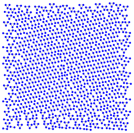
Figure 8. A random graph of size $n=1171$ with component size at most 3. Observe that most components have size 3, so that the root component is very likely to have size 3.

Proposition 22 (Size of the components — Graphs with small components).

The distribution of $S_{n}$ converges to a Dirac law at $k$:

$$\mathbb{P}(S_{n}=j)\rightarrow\begin{cases}1&\text{if $j=k$,}\\ 0&\text{otherwise.}\end{cases}$$

The same holds for the size $L_{n}$ of the largest component.

Proof.

We combine the second formulation in (2) with the estimate (26) of $a_{n}$. This gives

$$\mathbb{P}(S_{n}=j)\sim\frac{1}{n}\frac{c_{j}}{(j-1)!}\frac{A(\zeta_{n-j})}{A(\zeta_{n})}\frac{\zeta_{n}^{n}}{\zeta_{n-j}^{n-j}}.$$

Clearly, it suffices to prove that this probability tends to $0$ if $j<k$. So let us assume $j<k$. Since $\zeta_{n}$ is increasing with $n$, it suffices to prove that

$$\frac{1}{n}\frac{\zeta_{n}^{n}}{\zeta_{n-j}^{n-j}}\rightarrow 0.$$ (30)

Recall from (27) and (29) that $\zeta_{n}$ admits an expansion of the form

$$\zeta_{n}=\alpha{n^{1/k}}+\sum_{i=0}^{{k-1}}n^{-i/k}\beta_{i}+O\left(1/{n}\right).$$

This gives, for some constants $\gamma_{i}$,

$$n\log\zeta_{n}=\frac{n}{k}\log n+n\log\alpha+\sum_{i=1}^{k}\gamma_{i}n^{1-i/k}+O(n^{-1/k}).$$

Hence

$$(n-j)\log\zeta_{n-j}=\frac{n-j}{k}\log n+(n-j)\log\alpha+\sum_{i=1}^{k}\gamma_{i}n^{1-i/k}+O(1).$$

This gives

$$n\log\zeta_{n}-(n-j)\log\zeta_{n-j}-\log n=\frac{j-k}{k}\log n+O(1),$$

and (30) follows, since $j<k$. Since $L_{n}\geq S_{n}$, the behaviour of $L_{n}$ is then clear.  

8. Forests of paths or caterpillars: a simple pole in $\boldsymbol{C(z)}$

Let $\mathcal{A}$ be a decomposable class (for instance defined by excluding connected minors), with generating function $A(z)=\exp(C(z))$. Assume that

$$C(z)=\frac{\alpha}{1-z/\rho}+D(z),$$ (31)

where $D$ has radius of convergence larger than $\rho$. Of course, we assume $\alpha>0$.

Proposition 23 (The number of graphs — when $C$ has a simple pole).

Assume that the above conditions hold, and let $\beta=D(\rho)$. As $n\rightarrow\infty$,

$$c_{n}\sim n!\,\alpha\rho^{-n}\quad\hbox{and}\quad a_{n}\sim n!\,\frac{\alpha^{1/4}e^{\alpha/2+\beta}}{2\sqrt{\pi}n^{3/4}}\rho^{-n}e^{2\sqrt{\alpha n}}.$$ (32)

In particular, the probability that $\mathcal{G}_{n}$ is connected tends to $0$ at speed $n^{3/4}e^{-2\sqrt{\alpha n}}$.

Proof.

The asymptotic behaviour of $c_{n}$ follows from [19, Thm. IV.10, p. 258]. To obtain the asymptotic behaviour of $a_{n}$, we first write

$$A(z)=F(z)G(z)\hskip 14.22636pt\hbox{ with }\hskip 14.22636ptF(z)=\exp\left({\frac{\alpha}{1-z/\rho}}\right)\hskip 14.22636pt\hbox{ and }\hskip 14.22636ptG(z)=e^{D(z)},$$ (33)

where $G(z)$ has radius of convergence larger than $\rho$. To estimate the coefficients of $F$, we apply the ready-to-use results of Macintyre and Wilson [25, Eqs. (10)–(14)], according to which, for $\alpha,\gamma>0$ and a non-negative integer $k$,

$$[z^{n}]\left(\log\frac{1}{1-z}\right)^{k}\frac{1}{(1-z)^{\gamma}}\exp\left(\frac{\alpha}{1-z}\right)\sim\frac{\alpha^{1/4}e^{\alpha/2}}{2\sqrt{\pi}n^{3/4}}\left(\frac{n}{\alpha}\right)^{\gamma/2}\left(\frac{\log n}{2}\right)^{k}e^{2\sqrt{\alpha n}}.$$ (34)

This gives

$$f_{n}:=[z^{n}]F(z)\sim\frac{\alpha^{1/4}e^{\alpha/2}}{2\sqrt{\pi}n^{3/4}}\rho^{-n}e^{2\sqrt{\alpha n}}.$$

This shows in particular that $f_{n-1}/f_{n}$ tends to $\rho$ as $n\rightarrow\infty$, so that we can apply Proposition 19 to (33) and conclude.  

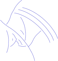
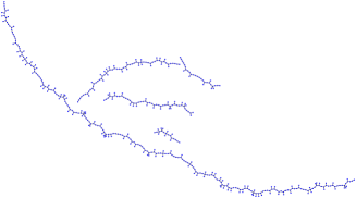
Figure 9. A random forest of paths of size $n=636$ (left) and a forest of caterpillars of size $n=486$ (right).

Proposition 24 (Number of components — when $C$ has a simple pole).

Assume (31) holds. The mean and variance of $N_{n}$ satisfy:

$$\mathbb{E}(N_{n})\sim\sqrt{\alpha n},\quad\quad\mathbb{V}(N_{n})\sim\sqrt{\alpha n}/2,$$

and the random variable $\frac{N_{n}-\sqrt{\alpha n}}{(\alpha n/4)^{1/4}}$ converges in law to a standard normal distribution.

Proof.

We apply Theorem 18. The H-admissibility of $A(z)$ follows from Theorem 17, using (33) and the H-admissibility of $\exp(\alpha/(1-z/\rho))$ (see [19, p. 562]). Conditions (19)–(21) are then readily checked, using

$$C(r)\sim\frac{\alpha}{1-r/\rho},\quad b(r)\sim\frac{2\alpha}{(1-r/\rho)^{3}}\quad\hbox{and}\quad V(r)\sim\frac{\alpha}{2(1-r/\rho)}.$$

We thus conclude that the normalized version of $N_{n}$ converges in law to a standard normal distribution. For the asymptotic estimates of $\mathbb{E}(N_{n})$ and $\mathbb{V}(N_{n})$, we use (22) with the saddle point estimate $\zeta_{n}=\rho-\rho\sqrt{\alpha/n}+O(1/n).$  

Since there are approximately $\sqrt{n}$ components, one may expect the size $S_{n}$ of the root component to be of the order of $\sqrt{n}$.

Proposition 25 (Size of the root component — when $C$ has a simple pole).

The normalized variable $S_{n}/\sqrt{n/\alpha}$ converges in distribution to a Gamma$(2,1)$ law of density $xe^{-x}$ on $[0,\infty)$. In fact, a local limit law holds: for $x>0$ and $k=\lfloor x\sqrt{n/\alpha}\rfloor$,

$$\sqrt{n/\alpha}\ \mathbb{P}(S_{n}=k)\rightarrow xe^{-x}.$$

The convergence of moments holds as well: for $i\geq 0$,

$$\mathbb{E}(S_{n}^{i})\sim(i+1)!(n/\alpha)^{i/2}.$$

Proof.

For the local (and hence global) limit law, we simply combine (2) with (32). For the moments, we start from (4), with

$$C^{(i+1)}(z)=\frac{\alpha(i+1)!}{\rho^{i+1}(1-z/\rho)^{i+2}}+D^{(i+1)}(z).$$

Let us first observe that (32) implies that $a_{n}/n!$ is smooth. We can thus apply Proposition 19 to the product $D^{(i+1)}(z)A(z)$, which gives

$$\frac{[z^{n-i-1}]D^{(i+1)}(z)A(z)}{n[z^{n}]A(z)}\sim\frac{D^{(i+1)}(\rho)}{n}\frac{a_{n-i-1}}{(n-i-1)!}\frac{n!}{a_{n}}\sim\frac{D^{(i+1)}(\rho)}{n}\rho^{i}\rightarrow 0.$$

We thus have

$$\frac{a_{n}}{(n-1)!}\,\mathbb{E}(S_{n}^{i})\sim[z^{n-i-1}]\frac{\alpha(i+1)!}{\rho^{i+1}(1-z/\rho)^{i+2}}\exp\left(\frac{\alpha}{1-z/\rho}+D(z)\right).$$ (35)

Now (34) gives

$$[z^{n-i-1}]\frac{\alpha(i+1)!}{\rho^{i+1}(1-z/\rho)^{i+2}}\exp\left(\frac{\alpha}{1-z/\rho}\right)\sim\alpha(i+1)!\,\frac{\alpha^{1/4}e^{\alpha/2}}{2\sqrt{\pi}n^{3/4}}\left(\frac{n}{\alpha}\right)^{i/2+1}\rho^{-n}e^{2\sqrt{\alpha n}}.$$ (36)

In particular, this sequence of coefficients is smooth. Hence by Proposition 19, the asymptotic behaviour of (35) only differs from (36) by a factor $e^{\beta}$, where $\beta=D(\rho)$. Combined with (32), this gives the limiting $i$th moment of $S_{n}$. Since these moments characterize the above Gamma distribution, we can conclude [19, Thm. C.2] that $S_{n}/\sqrt{n/\alpha}$ converges in law to this distribution.  

We now present two classes for which $C(z)$ has a simple isolated pole (Figure 9): forests of paths, and forests of caterpillars (a caterpillar is a tree made of a simple path to which leaves are attached; see Figure 1). In forests of paths, the excluded minors are the triangle $K_{3}$ and the 3-star. The fact that $N_{n}$ converges in probability to $\sqrt{n/2}$ for this class was stated in [26, p. 587]. For forests of caterpillars, the excluded minors are $K_{3}$ and the tree shown in Table 1 ($6$th line). This class is also considered in [6]. It is also the class of graphs of pathwidth 1.

Proposition 26 (Forests of paths or caterpillars).

The generating functions of paths and of caterpillars are respectively

$$C_{p}(z)=\frac{z(2-z)}{2(1-z)}\quad\quad\hbox{and}\quad\quad C_{c}(z)=\frac{z^{2}(e^{z}-1)^{2}}{2(1-ze^{z})}+ze^{z}-\frac{z^{2}}{2}.$$ (37)

For both series, Condition (31) is satisfied and Propositions 23, 24 and 25 hold. For paths we have $\rho=1$, $\alpha=1/2$ and $\beta:=D(\rho)=0$. For caterpillars, $\rho\simeq 0.567$ is the only real such that $\rho e^{\rho}=1$,

$$\alpha=\frac{(1-\rho)^{2}}{2(1+\rho)}\simeq 0.06\quad\hbox{and}\quad\beta={\frac{\rho\,\left(10+3\,\rho-4\,{\rho}^{2}-{\rho}^{3}\right)}{4\left(1+\rho\right)^{2}}}\simeq 0.59.$$ (38)

Proof.

The expression of $C_{p}(z)$ is straightforward. One can also write

$$C_{p}(z)=\frac{1}{2(1-z)}+\frac{z-1}{2},$$

which gives $D_{p}(1)=0$. Let us now focus on caterpillars. Let us call star a tree in which all vertices, except maybe one, have degree 1. By a rooted star we mean a star with a marked vertex of maximum degree: hence the root has degree 0 for a star with 1 vertex, 1 for a star with 2 vertices, and at least 2 otherwise. Clearly, there are $n$ rooted stars on $n$ labelled vertices, so that their generating function is

$$S^{\bullet}(z)=\sum_{n\geq 1}\frac{z^{n}}{(n-1)!}=ze^{z}.$$

The generating function of (unrooted) stars is

$$S(z)=S^{\bullet}(z)-\frac{z^{2}}{2}=ze^{z}-\frac{z^{2}}{2}$$

(because all stars have only one rooting, except the star on 2 vertices which has two). Now a caterpillar is either a star, or is a (non-oriented) chain of at least two rooted stars, the first and last having at least 2 vertices each. This gives

$$C(z)=S(z)+\frac{(S^{\bullet}(z)-z)^{2}}{2(1-S^{\bullet}(z))},$$

which is equivalent to the right-hand side of (37).

The series $C_{c}(z)$ is meromorphic on ${\mathbb{C}}$, with a unique dominant pole at $\rho$, and its behaviour around this point is easily found using a local expansion of $ze^{z}$ at $\rho$:

$$C_{c}(z)=\frac{\alpha}{1-z/\rho}+\beta+O\left(1-z/\rho\right),$$

with $\alpha$ and $\beta$ as in (38).  

For forests of paths, we have also obtained the limit law of the size $L_{n}$ of the largest component. It is significantly larger than the root component ($\sqrt{n}\log n$ instead of $\sqrt{n}$).

Proposition 27 (Size of the largest component — forests of paths).

In forests of paths, the (normalized) size of the largest component converges in law to a Gumbel distribution: for $x\in{\mathbb{R}}$ and as $n\rightarrow\infty$,

$$\mathbb{P}\left(\frac{L_{n}-\sqrt{n/2}\log n}{\sqrt{n/2}}<x\right)\rightarrow\exp\left(-\frac{e^{-x/2}}{\sqrt{2}}\right).$$

Proof.

We start from (5), where

$$k=\sqrt{n/2}\left(\log n+x\right)$$ (39)

and the generating function of paths of size less than $k$ is:

$$C^{[k]}(z)=\frac{z}{2}+\frac{z-z^{k}}{2(1-z)}.$$ (40)

Using a saddle point approach for integrals [19, p. 552], we will find an estimate of

$$[z^{n}]\exp(C^{[k]}(z))=\frac{1}{2i\pi}\int_{\mathcal{C}_{r}}\exp(C^{[k]}(z))\frac{dz}{z^{n+1}},$$ (41)

where the integration contour is any circle $\mathcal{C}_{r}$ of center $0$ and radius $r<1$.

Let us first introduce some notation: we denote $C^{[k]}(z)$ by $K(z)$, the integrand in  (41) by $F$, and its logarithm by $f$:

$$K(z)=C^{[k]}(z),\quad F(z)=\frac{\exp(K(z))}{z^{n+1}},\quad\quad f(z)=K(z)-(n+1)\log z.$$

We choose the radius $r\equiv r_{n}$ that satisfies the saddle point equation

$$F^{\prime}(r)=0,\quad\hbox{or equivalently}\quad f^{\prime}(r)=0\quad\hbox{or}\quad rK^{\prime}(r)=n+1.$$

Note that $rK^{\prime}(r)$ increases from $0$ to $\infty$ as $r$ grows from $0$ to $1$, so that the solution of this equation is unique and simple to approximate via bootstrapping. We find:

$$r=1-\frac{1}{\sqrt{2n}}+\frac{e^{-x/2}}{4\sqrt{2}}\frac{\log n}{n}+O\!\left(\frac{1}{n}\right).$$ (42)

Gaussian approximation. Let $\theta_{0}\in(0,\pi)$. By expanding the function $g:\theta\mapsto f(re^{i\theta})$ in the neighbourhood of $\theta=0$, we find, for $|\theta|\leq\theta_{0}$:

$$\left|f(re^{i\theta})-f(r)+\theta^{2}r^{2}f^{\prime\prime}(r)/2\right|\leq\frac{\theta_{0}^{3}}{6}\sup_{|\alpha|\leq\theta_{0}}\left|g^{(3)}(\alpha)\right|,$$ (43)

with

$$\left|g^{(3)}(\alpha)\right| = \left|-ire^{i\alpha}f^{\prime}(re^{i\alpha})-3ir^{2}e^{2i\alpha}f^{\prime\prime}(re^{i\alpha})-ir^{3}e^{3i\alpha}f^{\prime\prime\prime}(re^{i\alpha})\right|$$

$$\leq K^{\prime}(r)+\frac{n+1}{r}+3K^{\prime\prime}(r)+3\frac{n+1}{r^{2}}+K^{\prime\prime\prime}(r)+2\frac{n+1}{r^{3}}.$$

By combining the expression (40) of $K(z)=C^{[k]}(z)$ and the saddle point estimate (42), we find that $K^{\prime}(r)=(n+1)/r\sim n$, that $K^{\prime\prime}(r)\sim 2\sqrt{2}n^{3/2}$ and finally that $K^{\prime\prime\prime}(r)\sim 12n^{2}$. This term dominates the above bound on $|g^{(3)}(\alpha)|$. Hence, if

$$\theta_{0}\equiv\theta_{0}(n)=o(n^{-2/3}),$$ (44)

we find, by taking the exponential of (43),

$$F(re^{i\theta})\sim F(r)e^{-\theta^{2}r^{2}f^{\prime\prime}(r)/2},$$

uniformly in $|\theta|\leq\theta_{0}$.

Completion of the Gaussian integral. We split the integral (41) into two parts, depending on whether $|\theta|\leq\theta_{0}$ or $|\theta|\geq\theta_{0}$. The first part is

$$\int_{-\theta_{0}}^{\theta_{0}}F(re^{i\theta})\frac{re^{i\theta}d\theta}{2\pi}\sim\frac{rF(r)}{2\pi}\int_{-\theta_{0}}^{\theta_{0}}e^{-\theta^{2}r^{2}f^{\prime\prime}(r)/2}e^{i\theta}d\theta.$$

As argued above, $r^{2}f^{\prime\prime}(r)\sim K^{\prime\prime}(r)\sim 2\sqrt{2}n^{3/2}$. Hence, if we choose $\theta_{0}\equiv\theta_{0}(n)$ such that $\theta_{0}^{2}n^{3/2}\rightarrow\infty$ (which is compatible with (44), for instance if

$$\theta_{0}=n^{-5/7},$$ (45)

which we henceforth assume), we obtain

$$\int_{-\theta_{0}}^{\theta_{0}}F(re^{i\theta})\frac{re^{i\theta}d\theta}{2\pi} \sim \frac{F(r)}{2\pi\sqrt{f^{\prime\prime}(r)}}\int_{-\theta_{0}r\sqrt{f^{\prime\prime}(r)}}^{\theta_{0}r\sqrt{f^{\prime\prime}(r)}}e^{-\alpha^{2}/2}e^{i\alpha/(r\sqrt{f^{\prime\prime}(r)})}d\alpha$$ (46)

$$\sim \frac{F(r)}{2\pi\sqrt{f^{\prime\prime}(r)}}\int_{\mathbb{R}}e^{-\alpha^{2}/2}d\alpha$$

$$\sim \frac{F(r)}{\sqrt{2\pi f^{\prime\prime}(r)}}$$

$$\sim \frac{e^{1/4}e^{\sqrt{2n}}}{2^{1/4}2\sqrt{\pi}n^{3/4}}\exp\left(-\frac{e^{-x/2}}{\sqrt{2}}\right)$$

by (42).

The second part of the integral can be neglected. The second part of the integral (41) is

$$\int_{\theta_{0}<|\theta|<\pi}F(re^{i\theta})\frac{re^{i\theta}d\theta}{2\pi},$$

and we want to prove that it is dominated by (46). It suffices to prove that for $\theta_{0}<|\theta|<\pi$,

$$|F(re^{i\theta})|=o\left(\frac{F(r)}{\sqrt{f^{\prime\prime}(r)}}\right).$$ (47)

Let us denote $z=re^{i\theta}$ and $z_{0}=re^{i\theta_{0}}$. We have

$$\frac{|F(re^{i\theta})|}{F(r)} = |\exp(K(z)-K(r))|$$

$$\leq \exp(|K(z)|-K(r))=\exp\left(\left|\frac{z}{2}+\frac{z-z^{k}}{2(1-z)}\right|-\frac{r}{2}-\frac{r-r^{k}}{2(1-r)}\right)$$

$$\leq \exp\left(\frac{r+r^{k}}{2|1-z|}-\frac{r-r^{k}}{2(1-r)}\right)$$

$$\leq \exp\left(\frac{r+r^{k}}{2|1-z_{0}|}-\frac{r-r^{k}}{2(1-r)}\right)=\exp\left(-\frac{n^{1/14}}{\sqrt{2}}(1+o(1))\right),$$

given the values (39), (42) and (45) of $k$, $r$ and $\theta_{0}$. Since $f^{\prime\prime}(r)\sim 2\sqrt{2}n^{3/2}$, we conclude that (47) holds.

Conclusion. We have now established that the integral (41) is dominated by its first part, and is thus equivalent to (46). To obtain the limiting distribution function, it remains to divide this estimate by $a_{n}/n!$. The asymptotic behaviour of $a_{n}$ is given by (32), with $\alpha=1/2$, $\rho=1$ and $\beta=0$, and this concludes the proof.  

9. Graphs with maximum degree 2: a simple pole and a logarithm in $\boldsymbol{C(z)}$

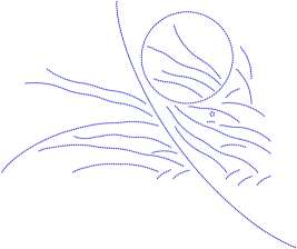
Figure 10. A random graph of size $n=1034$ avoiding the 3-star.

Let $\mathcal{A}$ be the class of graphs of maximum degree 2, or equivalently, the class of graphs avoiding the 3-star (Figure 10). The connected components of such graphs are paths or cycles. This class differs from those studied in the previous section in that the series $C(z)$ has now, in addition to a simple pole, a logarithmic singularity at its radius of convergence $\rho$. As we shall see, the logarithm changes the asymptotic behaviour of the numbers $a_{n}$, but the other results remain unaffected. The proofs are very similar to those of the previous section.

Proposition 28 (The number of graphs of maximum degree 2).

The number of connected graphs (paths or cycles) of size $n$ in the class $\mathcal{A}$ is $c_{n}=n!/2+(n-1)!/2$ for $n\geq 3$ (with $c_{1}=c_{2}=1$) and the associated generating function  is

$$C(z)=\frac{z(2-z+z^{2})}{4(1-z)}+\frac{1}{2}\log\frac{1}{1-z}.$$

The generating function of graphs of $\mathcal{A}$ is

$$A(z)=e^{C(z)}=\frac{1}{\sqrt{1-z}}\exp\left(\frac{z(2-z+z^{2})}{4(1-z)}\right).$$

As $n\rightarrow\infty$,

$$a_{n}\sim n!\,\frac{1}{2\sqrt{e\pi}n^{1/2}}e^{\sqrt{2n}}.$$

In particular, the probability that $\mathcal{G}_{n}$ is connected tends to $0$ at speed $n^{1/2}e^{-\sqrt{2n}}$ as $n\rightarrow\infty$.

Proof.

Again, the exact results are elementary. To obtain the asymptotic behaviour of $a_{n}$, we write

$$A(z)=F(z)G(z)\quad\hbox{with}\quad F(z)=\frac{1}{\sqrt{1-z}}\exp\left(\frac{1}{2(1-z)}\right)\quad\hbox{and}\quad G(z)=\exp\left(-\frac{1}{2}-\frac{z^{2}}{4}\right)$$ (48)

and combine Proposition 19 with (34).  

For the number of components, we find the same behaviour as in the case of a simple pole (Proposition 24 with $\alpha=1/2$). We have also determined the expected number of cyclic components.

Proposition 29 (Number and nature of components — Graphs of maximum degree 2).

The mean and variance of $N_{n}$ satisfy:

$$\mathbb{E}(N_{n})\sim\sqrt{n/2},\quad\quad\mathbb{V}(N_{n})\sim{\sqrt{n/8}},$$

and the random variable $\frac{N_{n}-\sqrt{n/2}}{(n/8)^{1/4}}$ converges in law to a standard normal distribution.

The expected number of cycles in $\mathcal{G}_{n}$ is of order $(\log n)/4$.

Proof.

We want to apply Theorem 18. To prove that $A(z)$ is Hayman-admissible, we apply Theorem 17 to (48). This reduces our task to proving that $F(z)$ is H-admissible, which is done along the same lines as [19, Ex. VIII.7, p. 562] (see also the footnote of [22, p. 92], and Lemma 1 in [17]). Conditions (19)–(21) are readily checked. The asymptotic estimates of $\mathbb{E}(N_{n})$ and $\mathbb{V}(N_{n})$ are obtained through (22), using the saddle point estimate $\zeta_{n}=1-1/\sqrt{2n}+O(1/n)$.

The bivariate generating function of graphs of $\mathcal{A}$, counted by the size (variable $z$) and the number of cycles (variable $v$) is

$$\tilde{A}(z,v)=\exp\left(z+\frac{z^{2}}{2(1-z)}+v\operatorname{Cyc}(z)\right),$$

where $\operatorname{Cyc}(z)$ is given by (8). By differentiating with respect to $v$, the expected number of cycles in $\mathcal{G}_{n}$ is found to be:

$$\frac{[z^{n}]\operatorname{Cyc}(z)A(z)}{[z^{n}]A(z)}.$$

The asymptotic behaviour of $[z^{n}]A(z)=a_{n}/n!$ has been established in Proposition 28. We determine an estimate of $[z^{n}]\operatorname{Cyc}(z)A(z)$ in a similar fashion, using a combination of Proposition 19 and (34). We find

$$[z^{n}]\operatorname{Cyc}(z)A(z)\sim\frac{\log n}{8\sqrt{e\pi}n^{1/2}}e^{\sqrt{2n}},$$

and the result follows.  

The size of the root component is still described by Proposition 25, with $\alpha=1/2$. The proof is very similar, with now

$$C^{(i+1)}(z)=\frac{i!}{2}\frac{2+i-z}{(1-z)^{i+2}}-\frac{1}{2}{\bf 1}_{i=1},$$

where ${\bf 1}_{i=1}$ is $1$ if $i=1$ and is 0 otherwise.  

10. Excluding the bowtie: a singularity in $\boldsymbol{(1-z/\rho)^{-1/2}}$

We now denote by $\mathcal{A}$ the class of graphs avoiding the bowtie (Figure 11). The following proposition answers a question raised in [27].

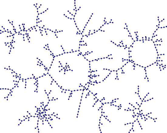
Figure 11. A random graph of size $n=758$ avoiding the bowtie.

Proposition 30 (The generating function  of graphs avoiding a bowtie).

Let $T\equiv T(z)$ be the generating function of rooted trees, defined by $T(z)=ze^{T(z)}$. The generating function of connected graphs in the class $\mathcal{A}$ is

$$C(z)={\frac{{T}^{2}\left(1-T+{T}^{2}\right){{\rm e}^{T}}}{1-T}}+\frac{1}{2}\log\left(\frac{1}{1-T}\right)+{\frac{T\left(12-54\,T+18\,{T}^{2}-5\,{T}^{3}-{T}^{4}\right)}{24(1-T)}}.$$ (49)

The generating function of graphs of $\mathcal{A}$ is $A(z)=e^{C(z)}.$

This is the most delicate enumeration of the paper. The key point is the following characterization of cores (graphs of minimum degree 2) avoiding the bowtie.

Proposition 31.

The cores that avoid the bowtie are:

• the empty graph,

• all cycles,

• $K_{4}$, with one edge possibly subdivided, as shown in Figure 16,

• the graphs of Figures 17 and 18.

We will first establish a number of properties of cores avoiding a bowtie. Recall that a chord of a cycle $C$ is an edge, not in $C$, joining two vertices of $C$.

Lemma 32.

Let $C=(v_{0},v_{1},\ldots,v_{n-1})$ be a cycle in a core $G$ avoiding the bowtie. Let us write $v_{n}=v_{0}$ and $v_{n+1}=v_{1}$. Every chord of $C$ joins vertices that are at distance $2$ on $C$ (we say that it is a short chord). Moreover, $C$ has at most two chords. If it has two chords, say $\{v_{0},v_{2}\}$ and $\{v_{i},v_{i+2}\}$, with $1\leq i\leq n-1$ , then $v_{i}=v_{1}$ or $v_{i+2}=v_{1}$.

Proof.

If a chord were not short, contracting it (together with some edges of $C$) would give a bowtie. Figure 12 then proves the second statement, which can be loosely restated as follows: the two chords cross and their four endpoints are consecutive on $C$.  

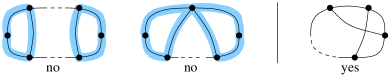
Figure 12. The relative positions of two (short) chords in a cycle. The first two configurations are not valid, as these graphs contain a bowtie (shown with gray/blue edges).

Lemma 33.

Let $C$ be a cycle of maximal length in a core $G$ avoiding the bowtie. Let $v$ be an external vertex, that is, a vertex not belonging to $C$. Then $v$ is incident to exactly two edges, both ending on $C$. The endpoints of these edges are at distance $2$ on $C$.

Proof.

Since $G$ is a core, $v$ belongs to a cycle $C^{\prime}$. Since $G$ is connected and avoids the bowtie, $C^{\prime}$ shares at least two vertices with $C$. Thus let $P_{1}$ and $P_{2}$ be two vertex-disjoint paths (taken from $C^{\prime}$) that start from $v$ and end on $C$ without hitting $C$ before. Let $v_{1}$ and $v_{2}$ be their respective endpoints on $C$. Then $v_{1}$ and $v_{2}$ lie at distance at least 2 on $C$, otherwise $C$ would not have maximal length. Now contracting the path $P_{1}P_{2}$ into a single edge gives a chord of $C$. By the previous lemma, this chord must be short, so that $v_{1}$ and $v_{2}$ are at distance exactly 2. Since $C$ has maximal length, $P_{1}$ and $P_{2}$ have length 1 each, and thus are edges.

Assume now that $v$ has degree at least 3, and let $e$ be a third edge (distinct from $P_{1}$ and $P_{2}$) adjacent to $v$. Again, $e$ must belong to a cycle, sharing at least two vertices with $C$, and the same argument as before shows that $e$ ends on $C$. But then Figure 13 shows that $G$ contains a bowtie.  

Figure 13. A cycle $C$ with an external vertex $v$ of degree at least 3. The cycle shown in gray/blue has a chord that is not short, the contraction of which gives a bowtie.

Lemma 34.

Let $C$ be a cycle of maximal length in a core $G$ avoiding the bowtie. If $C$ has two chords, it contains all vertices of $G$.

Proof.

Let $e_{1}$ and $e_{2}$ be the two chords of $C$. Lemma 32 describes their relative positions. Let $v$ be a vertex not in $C$. Lemma 33 describes how it is connected to $C$. Contract one of the two edges incident to $v$ to obtain a chord of $C$. By Lemma 32, this chord must be a copy of $e_{1}$ or $e_{2}$. But then Figure 14(a) shows that $G$ contains a bowtie (delete the two bold edges).  

Figure 14. A cycle $C$ with (a) two chords and an external vertex $v$ (b) one chord and an external vertex $v$.

Lemma 35.

Let $C$ be a cycle of maximal length in a core $G$ avoiding the bowtie. If $C$ has a chord $e$, all external vertices of $C$ are adjacent to the endpoints of $e$.

Proof.

Let $v$ be external to $C$. Contract one of the incident edges. This gives a chord $e^{\prime}$. If $e^{\prime}$ is a copy of $e$, then we are done. Otherwise, the relative positions of $e$ and $e^{\prime}$ are described by Lemma 32. But then Figure 14(b) shows that $C$ has not maximal length (consider the cycle shown with the dotted line).  

Lemma 36.

Let $C$ be a cycle of maximal length in a core $G$ avoiding the bowtie. If $C$ has several external vertices, they are adjacent to the same points of $C$.

Proof.

Consider two external vertices $v_{1}$ and $v_{2}$. Lemma 33 describes how each of them is connected to $C$. Contract an edge incident to $v_{1}$ and an edge incident to $v_{2}$. This gives two chords of $C$. Either these two chords are copies of one another, which means that $v_{1}$ and $v_{2}$ are adjacent to the same points of $C$. Or the relative position of these two chords is as described in Lemma 32. But then Figure 15 shows that $G$ contains a bowtie (contract $e$).  

Figure 15. A cycle $C$ with two external vertices.

Proof of Propositions 30 and 31.

Observe that a graph $G$ avoids the bowtie if and only if its core (defined as its maximal subgraph of degree 2) avoids it. Hence, if $\bar{C}(z)$ denotes the generating function of non-empty cores avoiding the bowtie, we have

$$C(z)=T(z)-\frac{T(z)^{2}}{2}+\bar{C}(T(z)).$$ (50)

Using the above lemmas, we can now describe and count non-empty cores avoiding the bowtie. We start with cores reduced to a cycle: their contribution to $\bar{C}(z)$ is given by (8). We now consider cores $G$ having several cycles. Let $C$ be a cycle of $G$ of maximal length, chosen so that it has the largest possible number of chords. By Lemma 32, this number is 2, 1 or 0.

If $C$ has two chords, it contains all vertices of $G$ (Lemma 34). By Lemma 32 and Figure 12 (right), either all vertices have degree 3 and $G=K_{4}$, or $G$ consists of $K_{4}$ where one edge is subdivided (Figure 16).

Figure 16. $K_{4}$ with a subdivided edge.

This gives the generating function

$$\frac{z^{4}}{4!}+\frac{z^{4}}{4!}\cdot 6\cdot\frac{z}{1-z},$$ (51)

where, in the second term, we read first the choice of the 4 vertices of degree 3 forming a $K_{4}$, then the choice of one edge of this $K_{4}$, and finally the choice of a (directed) path placed along this edge.

Assume now that $C$ has exactly one chord $e$. By Lemma 35, all external vertices are adjacent to the endpoints of $e$. To avoid problems with symmetries, we count separately the cores where $C$ has length $4$, or length $\geq 5$ (Figure 17). This gives the generating function

$$\frac{z^{2}}{2}(e^{z}-1-z)+\frac{z^{2}}{2}(e^{z}-1)\frac{z^{2}}{1-z}.$$ (52)

In the second term, the factor $z^{2}/(1-z)$ accounts for the directed chain of vertices of degree 2 lying on the maximal cycle.

Figure 17. A maximal cycle with one chord $e$ and external vertices.

Assume finally that $C$ has no chord. By Lemma 36, all external vertices are adjacent to the same points of $C$. Again, we treat separately the cases where $C$ has length $4$, or length $\geq 5$ (Figure 18). This gives the generating function

$$\frac{z^{2}}{2}(e^{z}-1-z-z^{2}/2)+\frac{z^{2}}{2}(e^{z}-1-z)\frac{z^{2}}{1-z}.$$ (53)

Figure 18. A maximal cycle $C$ with no chord and several external vertices.

Putting together the contributions (8), (51), (52) and (53) gives the value of $\bar{C}(z)$ (the generating function of cores) from which we obtain the series $C(z)$ using (50).  

We now derive asymptotic results from Proposition 30.

Proposition 37 (The asymptotic number of graphs avoiding the bowtie).

As $n\rightarrow\infty$,

$$c_{n}\sim n!\,\frac{e-5/4}{\sqrt{2\pi}}\frac{e^{n}}{\sqrt{n}}$$

and

$$a_{n}\sim n!\,\frac{(e-5/4)^{1/6}e^{{19}/8-{11e}/3}}{\sqrt{6\pi}}\frac{e^{n}}{{n}^{2/3}}\,\exp\left({\frac{3}{2}(e-5/4)^{2/3}n^{1/3}}\right).$$

Proof.

Let us first recall that the series $T(z)$ has radius of convergence $1/e$, and can be continued analytically on the domain $\mathcal{D}:={\mathbb{C}}\setminus[1/e,+\infty)$. In fact, $T(z)=-W(-z)$, where $W$ is the (principle branch of the) Lambert function [12]. The singular behaviour of $T(z)$ near $1/e$ is given by (6). Moreover, the image of $\mathcal{D}$ by $T$ avoids the half-line $[1,+\infty)$.

It thus follows from the expression (49) of $C(z)$ that $C(z)$ and $A(z)$ are analytic in the domain $\mathcal{D}$. Moreover, we derive from (6) that, as $z$ approaches $1/e$ in a $\Delta$-domain,

$$C(z)\sim\frac{e-5/4}{\sqrt{2}\sqrt{1-ze}}.$$ (54)

The above estimate of $c_{n}$ then follows from singularity analysis.

We now embark with the estimation of $a_{n}$. We first prove (see Proposition 40 in the appendix) that $A(z)$ is H-admissible. We then apply Theorem 16. The saddle point equation reads $\zeta C^{\prime}(\zeta)=n$. Using the singular expansion (6) of $T(z)$, and a similar expansion for $T^{\prime}(z)$, this reads

$$\frac{e-5/4}{2\sqrt{2}({1-\zeta e})^{3/2}}+\frac{1}{4({1-\zeta e})}+O\left(\frac{1}{({1-\zeta e})^{1/2}}\right)=n.$$ (55)

This gives the saddle point as

$$\zeta=\frac{1}{e}-\frac{(e-5/4)^{2/3}}{2en^{2/3}}-\frac{1}{6en}+O(n^{-4/3}).$$ (56)

We now want to obtain estimates of the values $A(\zeta)$, $\zeta^{n}$ and $b(\zeta)$ occurring in Theorem 16. Refining (54) into

$$C(z)=\frac{e-5/4}{\sqrt{2}\sqrt{1-ze}}+\frac{1}{4}\log\frac{1}{2(1-ze)}+\frac{19}{8}-\frac{11e}{3}+O(\sqrt{1-ze}),$$ (57)

we find

$$C(\zeta)=(e-5/4)^{2/3}n^{1/3}+\frac{1}{6}\log\frac{n}{e-5/4}+\frac{53}{24}-\frac{11e}{3}+O(n^{-1/3}),$$

which gives

$$A(\zeta)\sim\frac{e^{\frac{53}{24}-\frac{11e}{3}}}{(e-5/4)^{1/6}}{n^{1/6}}\exp((e-5/4)^{2/3}n^{1/3}).$$ (58)

It then follows from (56) that

$$\zeta^{n}\sim e^{-1/6}\exp\left(-n-(e-5/4)^{2/3}\,n^{1/3}/2\right).$$ (59)

Finally,

$$b(r)=rC^{\prime}(r)+r^{2}C^{\prime\prime}(r)\sim\frac{3\sqrt{2}(e-5/4)}{8(1-re)^{5/2}},$$ (60)

so that

$$b(\zeta)\sim\frac{3}{(e-5/4)^{2/3}}\,n^{5/3}.$$

Putting this estimate together with (58) and (59), we obtain the estimate of $a_{n}/n!$ given in the proposition.  

Proposition 38 (Number of components — no bowtie).

The mean and variance of $N_{n}$ satisfy:

$$\mathbb{E}(N_{n})\sim(e-5/4)^{2/3}n^{1/3},\quad\quad\mathbb{V}(N_{n})\sim\frac{2}{3}(e-5/4)^{2/3}n^{1/3},$$

and the random variable $\frac{N_{n}-\mathbb{E}(N_{n})}{\sqrt{\mathbb{V}(N_{n})}}$ converges in law to a standard normal distribution.

Proof.

We want to apply Theorem 18. By Proposition 40, $A(z)$ is H-admissible. Conditions (19)–(21) are readily checked, using

$$C(z)\sim\frac{e-5/4}{\sqrt{2}\sqrt{1-ze}},\quad b(r)\sim\frac{3\sqrt{2}(e-5/4)}{8(1-ze)^{5/2}}\quad\hbox{and}\quad V(r)\sim\frac{\sqrt{2}(e-5/4)}{3\sqrt{1-ze}}.$$

The asymptotic estimates of $\mathbb{E}(N_{n})$ and $\mathbb{V}(N_{n})$ are obtained through (22), using the saddle point estimate (56).  

Since there are approximately $n^{1/3}$ components, one may expect the size $S_{n}$ of the root component to be of the order of $n^{2/3}$. More precisely, we have the following result.

Proposition 39 (Size of the root component — no bowtie).

The normalized variable $(e-5/4)^{2/3}S_{n}/(2n^{2/3})$ converges in distribution to a Gamma$(3/2,1)$ law, of density $2\sqrt{x}e^{-x}/\sqrt{\pi}$ on $[0,\infty)$. In fact, a local limit law holds: for $x>0$ and $k=\lfloor x\frac{2n^{2/3}}{(e-5/4)^{2/3}}\rfloor$,

$$\frac{2n^{2/3}}{(e-5/4)^{2/3}}\ \mathbb{P}(S_{n}=k)\rightarrow 2\sqrt{\frac{x}{\pi}}e^{-x}.$$

The convergence of moments holds as well: for $i\geq 0$,

$$\mathbb{E}(S_{n}^{i})\sim\frac{\Gamma(i+3/2)}{\Gamma(3/2)}\left(\frac{2n^{2/3}}{(e-5/4)^{2/3}}\right)^{i}.$$

Proof.

The local (and hence global) limit law follows directly from Proposition 37, using (2). For the convergence of the moments, we start from (4). We first prove (see Proposition 40 in the appendix) that $C^{(i+1)}(z)A(z)$ is H-admissible. We then apply Theorem 16 to estimate the coefficient of $z^{n}$ in this series (we will replace $n$ ny $n-i-1$ later). Our calculations mimic those of Proposition 37, but the saddle point equation now reads

$$\zeta C^{\prime}(\zeta)+\zeta\,\frac{C^{(i+2)}(\zeta)}{C^{(i+1)}(\zeta)}=n,$$

where $\zeta\equiv\zeta_{n}^{(i)}$ depends on $i$ and $n$. Comparing with the original saddle point equation (55), and using the estimate (69) of $C^{(i)}(z)$, this reads

$$\frac{e-5/4}{2\sqrt{2}({1-\zeta e})^{3/2}}+\frac{7+4i}{4({1-\zeta e})}+O\left(\frac{1}{({1-\zeta e})^{1/2}}\right)=n.$$

This gives the saddle point as

$$\zeta=\frac{1}{e}-\frac{(e-5/4)^{2/3}}{2en^{2/3}}-\frac{7+4i}{6en}+O(n^{-4/3}).$$ (61)

We now want to obtain estimates of $C^{(i+1)}(\zeta)A(\zeta)$, $\zeta^{n}$ and $b_{i}(\zeta)$. We first derive from (57) that

$$C(\zeta)=(e-5/4)^{2/3}n^{1/3}+\frac{1}{6}\log\frac{n}{e-5/4}+\frac{29}{24}-\frac{11e}{3}-\frac{2i}{3}+O(n^{-1/3}).$$

This gives

$$A(\zeta)\sim\frac{e^{\frac{53}{24}-\frac{11e}{3}-\frac{2i}{3}}}{(e-5/4)^{1/6}}{n^{1/6}}\exp((e-5/4)^{2/3}n^{1/3}).$$ (62)

Moreover, we derive from (69) that

$$C^{(i+1)}(\zeta)\sim\frac{(2i+1)!}{2^{i}i!}e^{i+1}\frac{n^{1+2i/3}}{(e-5/4)^{2i/3}}.$$ (63)

It then follows from (61) that

$$\zeta^{n}\sim e^{-7/6-2i/3}\exp\left(-n-(e-5/4)^{2/3}\,n^{1/3}/2\right).$$ (64)

Finally, (71) and (60) give

$$b_{i}(\zeta)\sim b(\zeta)\sim\frac{3}{(e-5/4)^{2/3}}\,n^{5/3}.$$

Putting this estimate together with (62), (63) and (64), we obtain

$$[z^{n}]C^{(i+1)}(z)A(z)\sim\\ \frac{(2i+1)!}{2^{i}i!}\frac{(e-5/4)^{1/6}e^{{19}/8-{11e}/3}}{\sqrt{6\pi}}\frac{e^{n+i+1}}{{n}^{2/3}}\frac{n^{1+2i/3}}{(e-5/4)^{2i/3}}\,\exp\left({\frac{3}{2}(e-5/4)^{2/3}n^{1/3}}\right).$$

We finally replace $n$ by $n-i-1$ (the only effect is to replace $e^{n+i+1}$ by $e^{n}$), and divide by the estimate of $na_{n}/n!$ given in Proposition 37: this gives the estimate of the $i$th moment of $S_{n}$ as stated in the proposition, and concludes the proof.  

11. Final comments and further questions

11.1. Random generation

For each of the classes $\mathcal{A}$ that we have studied, we have designed an associated Boltzmann sampler, which generates a graph $G$ of $\mathcal{A}$ with probability

$$\mathbb{P}(G)=\frac{x^{|G|}}{|G|!A(x)},$$ (65)

where $x>0$ is a fixed parameter such that $A(x)$ converges. We refer to [18, Sec. 4] for general principles on the construction of exponential Boltzmann samplers, and only describe how we have addressed certain specific difficulties. Most of them are related to the fact that our graphs are unrooted.

Trees and forests. Designing a Boltzmann sampler for rooted trees is a basic exercise after reading [18]. Note that the calculation of $T(x)$ can be avoided by feeding the sampler directly with the parameter $t=T(x)$, taken in $(0,1]$. To sample unrooted trees, a first solution is to sample a rooted tree $G$ and keep it with probability $1/|G|$. However, this sometimes generates large rooted trees that are rejected with high probability. A much better solution is presented in [13, Sec. 2.2.1]. In order to obtain an unrooted tree distributed according to (65), one calls the sampler of rooted trees with a random parameter $t$. The density of $t$ must be chosen to be $(1-t)/C(x)$ on $[0,T(x)]$, with $C(x)=T(x)-T(x)^{2}/2$. To sample $t$ according to this density, we set $t=1-\sqrt{1-2uC(x)}$, where $u$ is uniform in $[0,1]$. Again, we actually avoid computing the series $C(x)$ by feeding directly our sampler with the value $T(x)\in(0,1]$. We use this trick for all classes that involve the series $T(x)$.

To obtain large forests (Figure 2), we actually sample forests with a distinguished vertex; that is, a rooted tree plus a forest [18, Sec. 6.3].

Paths, cycles and stars. The sequence operator of [18, Sec. 4] produces directed paths, while we need undirected paths. Let $u$ be uniform on $[0,1]$. Our generator generates the one-vertex path if $u<x/C_{p}(x)$, where $C_{p}(x)$ is given by (37), and otherwise generates a path of length $2+\operatorname{Geom}(x)$. An alternative is to generate a directed path, and reject it with probability $1/2$ if its size is at least 2.

Although the cycle operator of [18, Sec. 4] generates oriented cycles, this does not create a similar problem for our non-oriented cycles: indeed, a cycle of length at least 3 has exactly two possible orientations.

Designing a Boltzmann sampler $\Gamma RS$ for rooted stars is elementary. For unrooted stars, we simply call $\Gamma RS$, but reject the star with probability $1/2$ if it has size 2 (because the only star with two rootings has size 2).

Graphs avoiding the bowtie. This is the most complex of our algorithms, because the generation of connected graphs involves 7 different cases (see the proof of Proposition 30). There is otherwise no particular difficulty. We specialize this algorithm to the generation of graphs avoiding the 2-spoon (Proposition 11). However, the probability to obtain a forest is about $0.95$, and thus there is no point in drawing a random graph of this class.

The graphs shown in the paper have been drawn with the graphviz software.

11.2. The nature of the dominant singularities of $\boldsymbol{C(z)}$

This is clearly a crucial point, as the probability that $\mathcal{G}_{n}$ is connected and the quantities $N_{n}$ and $S_{n}$ seem to be directly correlated to it (see the summary of our results in Table 1). This raises the following question: is it possible to describe an explicit correlation between the properties of the excluded minors and the nature of the dominant singularities of $C(z)$? For instance, it is known that $C(\rho)$ is finite when all excluded minors are 2-connected, but Section 4 shows that this happens as well with some non-2-connected excluded minors. Which excluded minors give rise to a simple pole in $C(z)$ (as in caterpillars)? or to a logarithmic singularity (as for graphs with no bowtie nor diamond), or to a singularity in $(1-z/\rho)^{-1/2}$ (as for graphs with no bowtie)?

Some classes for which $C(z)$ has a unique dominant pole of high order are described in the next subsection.

11.3. More examples and predictions

Our examples, as well as a quick analysis, lead us to predict the following results when $C(z)$ has a unique dominant singularity and a singular behaviour of the form $(1-z/\rho)^{-\alpha}$, with $\alpha>0$:

• the mean and variance of the number $N_{n}$ of components scale like $n^{\alpha/(1+\alpha)}$, and $N_{n}$ admits a gaussian limit law after normalization,

• the mean of $S_{n}$ scales like $n^{1/(1+\alpha)}$, and $S_{n}$, normalized by its expectation, converges to a Gamma distribution of parameters $\alpha+1$ and $1$.

The second point is developed in [10]. To confirm these predictions one could study the following classes, which yield series $C(z)$ with a high order dominant pole. Fix $k\geq 2$, and consider the class $\mathcal{A}^{(k)}$ of forests of degree at most $k$, in which each component has at most one vertex of degree $\geq 3$. This means that the components are stars with long rays and “centers” of degree at most $k$. It is not hard to see that

$$C^{(k)}(z)=z+\frac{z^{2}}{2(1-z)}+\sum_{i=3}^{k}\frac{z^{i+1}}{i!(1-z)^{i}},$$

so that $C_{k}$ has a pole of order $k$ (for $k\geq 3$). The case $k=2$ corresponds to forests of paths (Section 8). The limit case $k=\infty$ (forests of stars with long rays) looks interesting, with a very fast divergence of $C$ at 1:

$$C^{(\infty)}(z)=z\exp\left(\frac{z}{1-z}\right)-\frac{z^{2}}{2(1-z)^{2}}.$$

We do not dare any prediction here.

11.4. Other parameters

We have focussed in this paper on certain parameters that are well understood when all excluded minors are 2-connected. But other parameters — number of edges, size of the largest 2-connected component, distribution of vertex degrees — have been investigated in other contexts, that sometimes intersect the study of minor-closed classes [8, 7, 14, 15, 20]. When specialized to the theory of minor-closed classes, these papers generally assume that all excluded minors are 2-connected, sometimes even 3-connected.

Clearly, it would not be hard to keep track of the number of edges in our enumerative results. Presumably, keeping track of the number of vertices of degree $d$ for any (fixed) $d$ would not be too difficult either. This may be the topic of future work. The size of the largest component clearly needs a further investigation as well.

Acknowledgements. KW would like to thank Colin McDiarmid for many inspiring and helpful discussions as well as for constant support. We also thank Philippe Duchon and Carine Pivoteau for their help with Boltzmann samplers, Nicolas Bonichon for a crash course on the Graphviz software, Jean-François Marckert for pointing out the relevance of [2] and finally Bruno Salvy for pointing out Reference [25].

We also thank the referees for their careful and detailed reports.

$$\triangleleft\;\lhd\;\diamond\;\rhd\;\triangleright$$

Appendix: Hayman-admissibility for bowties

Proposition 40.

Let $C(z)$ and $A(z)$ be the series given in Proposition 30. Then the series $A(z)$ and $C^{(i+1)}(z)A(z)$ are H-admissible, for any $i\geq 1$.

Proof.

We begin with the series $A(z)$. Recall the analytic properties of $T(z)$, listed at the beginning of the proof of Proposition 37. The capture condition ${\bf H_{1}}$ is readily checked. In fact,

$$a(r)=rC^{\prime}(r)\sim\frac{e-5/4}{2\sqrt{2}({1-re})^{3/2}}\quad\hbox{and}\quad b(r)=rC^{\prime}(r)+r^{2}C^{\prime\prime}(r)\sim\frac{3\sqrt{2}(e-5/4)}{8(1-re)^{5/2}}.$$ (66)

Let us now prove ${\bf H_{2}}$. By Taylor’s formula applied to the function $f:\theta\mapsto C(re^{i\theta})$, we have, for $r\in(0,1/e)$ and $\theta\in[-\theta_{0},\theta_{0}]$:

$$\left|C(re^{i\theta})-C(r)-i\theta a(r)+\theta^{2}b(r)/2\right|\leq|\theta_{0}^{3}|/6\sup_{|\alpha|\leq\theta_{0}}|f^{(3)}(\alpha)|$$

with

$$\left|f^{(3)}(\alpha)\right| = \left|-ire^{i\alpha}C^{\prime}(re^{i\alpha})-3ir^{2}e^{2i\alpha}C^{\prime\prime}(re^{i\alpha})-ir^{3}e^{3i\alpha}C^{\prime\prime\prime}(re^{i\alpha})\right|$$

$$\leq rC^{\prime}(r)+3r^{2}C^{\prime\prime}(r)+r^{3}C^{\prime\prime\prime}(r)\sim\frac{\kappa}{(1-re)^{7/2}}$$

as $r\rightarrow 1/e$, for some constant $\kappa$. Hence, if we take $\theta_{0}\equiv\theta_{0}(r)=o((1-re)^{7/6})$, then

$$\sup_{|\theta|\leq\theta_{0}(r)}\left|\frac{A(re^{i\theta})}{A(r)}e^{-i\theta a(r)+\theta^{2}b(r)/2}-1\right|=\left|e^{o(1)}-1\right|\rightarrow 0$$

as $r\rightarrow 1/e$. Thus ${\bf H_{2}}$ holds for such values of $\theta_{0}$. We now take

$$\theta_{0}(r)=(1-re)^{6/5},$$ (67)

and want to prove that ${\bf H_{3}}$ also holds.

Recall that $C(z)$ is analytic on ${\mathbb{C}}\setminus[1/e,\infty)$, and let us isolate in $C(z)$ the part that diverges at $z=1/e$:

$$C(z)=\frac{c}{\sqrt{1-ze}}+\frac{1}{4}\log\frac{1}{1-ze}+O(1)$$ (68)

where $c=({e-5/4})/{\sqrt{2}}>0.$ It follows that

$$B(z):=C(z)-\frac{c}{\sqrt{1-ze}}-\frac{1}{4}\log\frac{1}{1-ze}$$

is uniformly bounded on $\{|z|<1/e\}$. Hence, writing $z=re^{i\theta}$, we have

$$\sup_{|\theta|\in[\theta_{0},\pi)}\left|\frac{A(z)}{A(r)}\sqrt{b(r)}\right|\leq M\sup_{|\theta|\in[\theta_{0},\pi)}\left|\frac{1-re}{1-ze}\right|^{1/4}\left|\exp\left(\frac{c}{\sqrt{1-ze}}-\frac{c}{\sqrt{1-re}}\right)\right|\sqrt{b(r)}$$

for some constant $M$.

For any $z$ of modulus $r<1/e$, we have $|1-re|\leq|1-ze|$, and we can bound the first factor above by 1. Also, it is not hard to prove that $\Re\left(1/\sqrt{1-ze}\right)$ is a decreasing function of $\theta\in(0,\pi)$. Hence, denoting $z_{0}=re^{i\theta_{0}}$:

$$\sup_{|\theta|\in[\theta_{0},\pi)}\left|\frac{A(z)}{A(r)}\sqrt{b(r)}\right|\leq M\exp\left(\Re\left(\frac{c}{\sqrt{1-z_{0}e}}\right)-\frac{c}{\sqrt{1-re}}\right)\sqrt{b(r)}.$$

But as $r\rightarrow 1/e$, the choice (67) of $\theta_{0}$ implies that

$$\Re\left(\frac{c}{\sqrt{1-z_{0}e}}\right)-\frac{c}{\sqrt{1-re}}=-\frac{3c}{8(1-re)^{1/10}}+o(1).$$

Condition ${\bf H_{3}}$ now follows, using the estimate (66) of $b(r)$.

Let us now consider the series $A_{i}(z):=C^{(i+1)}(z)A(z)$, for $i\geq 1$. It is easy to prove by induction on $i$ that for $i\geq 1$,

$$C^{(i)}(z)=\frac{(2i)!(e-5/4)e^{i}}{4^{i}\sqrt{2}i!(1-ze)^{i+1/2}}+O\left(\frac{1}{(1-ze)^{i}}\right).$$ (69)

This can be proved either from the expression of $C(z)$ given in Proposition 30, or by starting from the singular expansion (68) of $C(z)$ and applying [19, Thm. VI.8, p. 419].

Recall the behaviour (66) of the functions $a(r)$ and $b(r)$ associated with $A(z)$. It follows, with obvious notation, that as $r\rightarrow 1/e$,

$$a_{i}(r)=a(r)+r\frac{C^{(i+2)}(r)}{C^{(i+1)}(r)}=a(r)+O\left(\frac{1}{1-re}\right)$$ (70)

and

$$b_{i}(r)=b(r)+r\frac{C^{(i+2)}(r)}{C^{(i+1)}(r)}+r^{2}\frac{C^{(i+3)}(r)}{C^{(i+1)}(r)}-r^{2}\left(\frac{C^{(i+2)}(r)}{C^{(i+1)}(r)}\right)^{2}=b(r)+O\left(\frac{1}{(1-re)^{2}}\right)$$ (71)

both tend to infinity. Thus ${\bf H_{1}}$ holds.

Let us now prove that $A_{i}(z)$ satisfies ${\bf H_{2}}$ with the same value of $\theta_{0}$ as for $A(z)$ (that is, $\theta_{0}=(1-re)^{6/5}$). Thanks to (70–71) we have, for $|\theta|\leq\theta_{0}$ and uniformly in $\theta$,

$$e^{-i\theta a_{i}(r)+\theta^{2}b_{i}(r)/2}=e^{-i\theta a(r)+\theta^{2}b(r)/2}\left(1+O((1-re)^{1/5})\right).$$

Now using (69), we obtain, denoting $z=re^{i\theta}$,

$$\frac{C^{(i+1)}(z)}{C^{(i+1)}(r)}=\left(\frac{1-ze}{1-re}\right)^{-i-3/2}\left(1+O((1-re)^{1/2})\right)=1+O((1-re)^{1/5}).$$

Hence

$$\frac{A_{i}(z)}{A_{i}(r)}e^{-i\theta a_{i}(r)+\theta^{2}b_{i}(r)/2}=\frac{A(z)}{A(r)}e^{-i\theta a(r)+\theta^{2}b(r)/2}\left(1+O((1-re)^{1/5})\right)$$

and Condition ${\bf H_{2}}$ holds for $A_{i}$ since it holds for $A$.

Finally, since $C(z)$ has non-negative coefficients, we have $\left|C^{(i+1)}(z)\right|\leq C^{(i+1)}(r)$ for $z=re^{i\theta}$. Thus the fact that $A_{i}(z)$ satisfies ${\bf H_{3}}$ follows from the fact that $A(z)$ satisfies ${\bf H_{3}}$, together with $b_{i}(r)\sim b(r)$.

References

- [1] L. Addario Berry, C. McDiarmid, and B. Reed. Connectivity for bridge-addable monotone graph classes. Combin. Probab. Comput., 21(6):803–815, 2012.
- [2] R. Arratia, A. D. Barbour, and S. Tavaré. Logarithmic combinatorial structures: a probabilistic approach. EMS Monographs in Mathematics. European Mathematical Society (EMS), Zürich, 2003.
- [3] C. Banderier, P. Flajolet, G. Schaeffer, and M. Soria. Random maps, coalescing saddles, singularity analysis, and Airy phenomena. Random Structures Algorithms, 19(3-4):194–246, 2001.
- [4] J. P. Bell, E. A. Bender, P. J. Cameron, and L. B. Richmond. Asymptotics for the probability of connectedness and the distribution of number of components. Electron. J. Combin., 7:Research Paper 33, 22 pp. (electronic), 2000.
- [5] E. A. Bender. Asymptotic methods in enumeration. SIAM Rev., 16:485–515, 1974.
- [6] O. Bernardi, M. Noy, and D. Welsh. Growth constants of minor-closed classes of graphs. J. Combin. Theory Ser. B, 100(5):468–484, 2010.
- [7] N. Bernasconi, K. Panagiotou, and A. Steger. On the degree sequences of random outerplanar and series-parallel graphs. In Approximation, randomization and combinatorial optimization, volume 5171 of Lecture Notes in Comput. Sci., pages 303–316. Springer, Berlin, 2008.
- [8] N. Bernasconi, K. Panagiotou, and A. Steger. The degree sequence of random graphs from subcritical classes. Combin. Probab. Comput., 18(5):647–681, 2009.
- [9] P. Billingsley. Convergence of probability measures. Wiley Series in Probability and Statistics: Probability and Statistics. John Wiley & Sons Inc., New York, second edition, 1999.
- [10] M. Bousquet-Mélou and K. Weller. Size of the root component in exponential structures. In preparation.
- [11] E. R. Canfield. Central and local limit theorems for the coefficients of polynomials of binomial type. J. Combinatorial Theory Ser. A, 23(3):275–290, 1977.
- [12] R. M. Corless, G. H. Gonnet, D. E. G. Hare, D. J. Jeffrey, and D. E. Knuth. On the Lambert function. Adv. Comput. Math., 5(4):329–359, 1996.
- [13] A. Darrasse, K. Panagiotou, O. Roussel, and M. Soria. Biased Boltzmann samplers and generation of extended linear languages with shuffle. In Proceedings of the 23rd International Meeting on Probabilistic, Combinatorial, and Asymptotic Methods in the Analysis of Algorithms (AofA’12), pages 125–140. Discrete Mathematics and Theoretical Computer Science, 2012.
- [14] M. Drmota, É. Fusy, M. Kang, V. Kraus, and J. Rué. Asymptotic study of subcritical graph classes. SIAM J. Discrete Math., 25(4):1615–1651, 2011.
- [15] M. Drmota, O. Giménez, and M. Noy. Degree distribution in random planar graphs. J. Combin. Theory Ser. A, 118(7):2102–2130, 2011.
- [16] M. Drmota, B. Gittenberger, and T. Klausner. Extended admissible functions and Gaussian limiting distributions. Math. Comp., 74(252):1953–1966 (electronic), 2005.
- [17] M. Drmota and M. Soria. Marking in combinatorial constructions: generating functions and limiting distributions. Theoret. Comput. Sci., 144(1-2):67–99, 1995.
- [18] P. Duchon, P. Flajolet, G. Louchard, and G. Schaeffer. Boltzmann samplers for the random generation of combinatorial structures. Combin. Probab. Comput., 13(4-5):577–625, 2004.
- [19] P. Flajolet and R. Sedgewick. Analytic combinatorics. Cambridge University Press, Cambridge, 2009.
- [20] O. Giménez, M. Noy, and J. Rué. Graph classes with given 3-connected components: Asymptotic enumeration and random graphs. Random Structures Algorithms, 42(4):438–479, 2013.
- [21] X. Gourdon. Largest component in random combinatorial structures. Discrete Math., 180(1-3):185–209, 1998.
- [22] W. K. Hayman. A generalisation of Stirling’s formula. J. Reine Angew. Math., 196:67–95, 1956.
- [23] M. Kang and K. Panagiotou. On the connectivity of random graphs from addable classes. J. Combin. Theory Ser. B, 103(2):306–312, 2013.
- [24] V. F. Kolchin. Random graphs, volume 53 of Encyclopedia of Mathematics and its Applications. Cambridge University Press, Cambridge, 1999.
- [25] A. J. Macintyre and R. Wilson. Operational methods and the coefficients of certain power series. Math. Ann., 127:243–250, 1954.
- [26] C. McDiarmid. Random graphs from a minor-closed class. Combin. Probab. Comput., 18(4):583–599, 2009.
- [27] C. McDiarmid. On graphs with few disjoint -star minors. European J. Combin., 32(8):1394–1406, 2011.
- [28] C. McDiarmid, A. Steger, and D. J. A. Welsh. Random planar graphs. J. Combin. Theory Ser. B, 93(2):187–205, 2005.
- [29] C. McDiarmid, A. Steger, and D. J. A. Welsh. Random graphs from planar and other addable classes. In Topics in discrete mathematics, volume 26 of Algorithms Combin., pages 231–246. Springer, Berlin, 2006.
- [30] S. Norine, P. Seymour, R. Thomas, and P. Wollan. Proper minor-closed families are small. J. Combin. Theory Ser. B, 96(5):754–757, 2006.
- [31] A. Rényi. On connected graphs. I. Magyar Tud. Akad. Mat. Kutató Int. Közl., 4:385–388, 1959.
- [32] N. Robertson and P.D. Seymour. Graph minors I–XX. J. Combin. Theory Ser. B, 1983–2004.
- [33] R. P. Stanley. Enumerative combinatorics. Vol. 2, volume 62 of Cambridge Studies in Advanced Mathematics. Cambridge University Press, Cambridge, 1999.
- [34] E. M. Wright. The number of connected sparsely edged graphs. J. Graph Theory, 1(4):317–330, 1977.