Critical study of hierarchical lattice renormalization group in magnetic ordered and quenched disordered systems: Ising and Blume-Emery-Griffiths models

Abstract

Renormalization group on hierarchical lattices is often considered a valuable tool to understand the critical behavior of more complicated statistical mechanical models. In presence of quenched disorder, however, in many model cases predictions obtained with the Migdal-Kadanoff bond removal approach fail to quantitatively and qualitatively reproduce critical properties obtained in the mean-field approximation or by numerical simulations in finite dimensions. In order to critically review this limitation we analyze the behavior of Ising and Blume-Emery-Griffiths models on more complicated hierarchical lattices. We find that, apart from some exceptions, the different behavior appears not only limited to Midgal-Kadanoff-like cells but is associated right to the hierarchization of Bravais lattices in small cells also when in-cell loops are considered.

1 Introduction

In this work we shall investigate the renormalization group analysis on spin systems with quenched disorder on hierarchical lattices. We will consider both Migdal-Kadanoff (MK) as well as more complex hierarchical lattices and we will study the critical behavior of systems with magnetic interactions in presence of random fields and random exchange interactions.

Our main aim is to investigate whether hierarchical cells more complicated than MK ones and more similar to the local structure of short-range Bravais lattices can reproduce features of ferromagnets and spin-glasses so far unobserved in position space renormalization group studies with MK lattices. In order to obtain a more general comprehension of the effect of bond moving we will provide estimates for critical quantities on several hierarchical lattices with different topology and compare them to known analytic and numerical results, when available.

Particular attention will be devoted to spin-glasses. Understanding the nature of the low temperature phase of spin-glasses in finite dimensional systems has turned out to be an extremely difficult task. Since the resolution of its mean-field approximation, valid above the upper critical dimension ($D=6$), more than thirty years have passed without a final word about the possible generalization of mean-field properties of spin-glasses to finite dimensional cases. The mean-field, else called Replica Symmetry Breaking (RSB) theory Parisi79 ; Parisi80 involves a very interesting solution for the spin-glass phase and its critical properties, rich of physical (and mathematical) implications, and has been fundamental in solving very diverse problems both in physics and in other disciplines Mezard87 ; Amit92 ; Mezard09 . Because of its complicated structure, to overcome technical (maybe also conceptual) obstacles hindering the “portability” of RSB theory predictions to short-range systems on Bravais lattice in $D<6$ is a rather big challenge in theoretical physics. Indeed, the RSB solution is so complex that non-perturbative effects cannot be taken under control in any perturbative loop-expansion around the upper critical dimension and critical scaling behavior is yet to be understood Chen77 ; DeDometal98 ; DeDominicis06 ; BraMoo11a ; ParTem12a ; SteNew12 . The main hindrance is the lack of translational invariance in the position space for locally frustrated systems with quenched disordered interactions, making the techniques developed for quantum field theory and successfully exported to statistical mechanical problems AmitBook ; LeBellacBook (e.g., for the Ising model critical exponents) inapplicable.

For what concerns Kadanoff original approach in position space Kadanoff ; Ma76 , a proper extension of renormalization group techniques to disordered and locally frustrated systems is still on its way. The generalization of classic position space renormalization methods on Bravais lattices to disordered interaction, such as the ones proposed for Ising spin models in the seventies Niemeijer73 ; Berker76 , has led to controversial results. On the one hand, by means of a cumulant expansion approach, evidence for a spin-glass phase is yielded in dimension two Kinzel78 ; Tatsumi78 , lower than the lower critical dimension on the Bravais lattice: $D=2.5$ Franz94 ; Franz05b ; Boettcher05 . On the other hand, the renormalization through block transformation on spin clusters does not yield any spin-glass fixed point even in dimension three Kinzel78 .

The only results have been achieved using “realizable” approximations, namely those that are the exact solution of some alternative problem. The first and most famous example is that of the classic “bond-moving” approximate Migdal-Kadanoff transformation, that when applied to Ising models on Bravais lattices provides the exact solution for an Ising model on a very different lattice, Berker_79 known as “hierarchical” lattices KG_82 . Note that, because of the “bond-moving” procedure, the hierarchical lattices corresponding to MK transformation (MK lattices in the following) have basically a 1D topology, as, e.g., the “necklace” lattice in Fig 2.

Therefore, most of the position space renormalization group (PSRG) studies have been concentrating on hierarchical lattices for which, in the ordered cases, the renormalization group flow is indeed exact (no truncation required). The study of these systems has brought to important results, cf., e.g., Refs. Berker_79 ; Berker_82 ; Ohzeki08 ; Salmon10 and references therein.

However, MK lattices fail to represent short-range spin-glasses on Bravais lattices also in the mean-field approximation and are, thus, strongly limited in probing the actual nature of the spin-glass phase Moore98 ; Ricci00 . For what concerns perturbative disorder in ferromagnetic systems, it has been found that the Nishimori conjecture does not provide the exact value of the multicritical point coordinate, Nobre01 ; Ohzeki08 although recently Ohzeki, Nishimori and Berker Ohzeki08 ; Nishimori10 have put forward an improved conjecture for models defined on hierarchical lattices and they found that for various families of these models a noteworthy recovery is obtained.

Furthermore the lack of translational invariance on hierarchical lattices is supposed to make peculiarly difficult the study of first order transitions. In particular, for pure fixed points while the expected first order transition is obtained in some model (see for example Berker81 ; Ozcelik08 ), there are relevant cases in which the corresponding transition is missing on MK lattices Tsallis84 ; Tsallis_96 . For what concerns disordered systems, MK lattices do not yield the first order fixed distribution expected for the random Blume-Emery-Griffiths model Ozcelik08 , as obtained both in mean-field theory Crisanti05b and by numerical simulations in finite dimension Paoluzzi10 . We stress as in the latter case the MK lattices neither show the expected re-entrance in the phase diagram Ozcelik08 ; Crisanti05b ; Paoluzzi10 .

Our aim is to test whether and which of the above mentioned differences are specifically due to the bond moving procedure at the basis of the renormalization group analysis. We will, thus, implement and compare the analysis of the critical behavior of well known statistical mechanical models with quenched field and bond randomness on both MK hierarchical lattices and the more complex “folded hierarchical lattices”, as we will call them.

The latter family consists of hierachical lattices obtained applying the two root reduction directly to the Bravais lattice Tsallis_96 (see Figs. 1, 3, 4, 5, 11), without the bond moving specific of the Migdal-Kadanoff transformation. So the final lattice has no longer just a 1D topology, but retains, in a small scale, the basic topology of the original lattice. So, unlike the MK family, in this case the original lattice is continuously reconstructed in the limit in which the length of the basic cell, called $b$ in the following (see Sec. 3), goes to infinity: the original lattice is a folded hierarchical lattice with an infinite basic cell.

In the following, we will first critically revisit, in each model case, the analyses on hierarchical lattices carried out in the literature. We will, then, compare those results to the outcome of our studies on more complex lattices in the family of folded cells.

The paper is organized as follows: in Sec. 2 we recall the implementation of the PSRG in the ferromagnetic Ising model. In Sec. 3 we expose the details of the generalization of the PSRG in presence of generic quenched disorder. In Sec. 3.1, we investigate the random field Ising model (RFIM) and in Secs. 3.2 and 3.3 we report on the Ising spin-glass, respectively below and above the lower critical dimension. We present and compare the estimates of critical parameters and discuss how they comply to known statistical mechanical criteria in presence of disorder (Nishimori conjecture, Harris criterion, ferromagnetic line inversion, $\ldots$). In Sec. 4 we consider the Blume-Emery-Griffiths model on several hierarchical lattices in dimension $d\geq 3$. In the latter case our analysis shows a phase diagram displaying a reentrance for strong disorder, absent on MK lattices Ozcelik08 , but present in the mean-field approximation Crisanti05 and in numerical simulations on 3D cubic lattices Paoluzzi10 ; Leuzzi11 ; Paoluzzi11 .

2 Hierarchical renormalization: Ising model

The Position Space Renormalization Group (PSRG) approach, approximated on realistic Bravais lattices, becomes exact when iterated on Hierarchical Lattices (HL) Migdal ; Kadanoff ; Berker_79 ; KG_82 ; Tsallis_96 . These lattices are constructed by carrying successive similar operations at each hierarchical level. E.g., at each level one replaces bonds by well-defined unit cells. See, for example, Fig. 1 for the diamond lattice or Fig. 2 for a MK lattice. The PSRG procedure works the inverse way of the lattice generation, i.e., one can implement it through a decimation of the internal sites of a given cell, leading to renormalized quantities associated with the external sites.

In the pure case, the PSRG analysis proceeds as known by finding the interactions leaving the partition function invariant under decimation, and obtaining the critical exponents by the eigenvalues of the first derivative matrix computed on the relative fixed point Cardy_book .

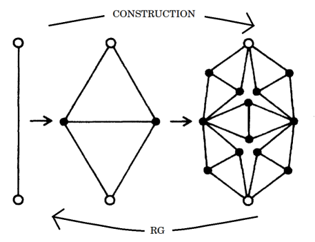
Figure 1: Costruction of diamond, else called 2-dimensional Wheatstone-bridge, hierarchical lattice with fractal dimension $d=\log 5/\log 2=2.3219\ldots$.

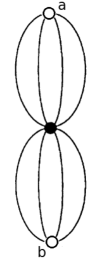
Figure 2: Necklace MK lattice. It has $b=2$ and fractal dimension $d=3$.

The well known Ising model is defined by the Hamiltonian

$$-{\cal{H}}(s)=J\sum_{\langle ij\rangle}s_{i}s_{j}+h\sum_{i}s_{i},$$ (1)

where $s_{i}=\pm 1$ and $\langle ij\rangle$ indicates a sum over nearest-neighbor pairs. We stress that here and in the rest of the paper we include the temperature in the definition of the couplings (reduced parameters).

Since we, eventually, want to study the critical properties of disordered systems, and since through the renormalization group transformation original random bonds induce random fields (and vice-versa) already at the first step of renormalization, it becomes more convenient to start using the following Hamiltonian

$$-\mathcal{H}(s)=\sum_{\langle ij\rangle}\left[J_{ij}s_{i}s_{j}+h_{ij}\frac{s_{i}+s_{j}}{2}+h_{ij}^{\dagger}\frac{s_{i}-s_{j}}{2}\right]$$ (2)

In this way each link between two sites $i$ and $j$ is associated with three (possibly disordered) interactions $J_{ij}$, $h_{ij}$ and $h_{ij}^{\dagger}$.

Decimating the inner sites $\{s\}$ of the basic cell ${\cal C}_{ab}$ of the hierarchical lattice with external sites $s_{a}$ and $s_{b}$, while imposing the conservation of the partition function of the cell

$$Z_{{\cal C}_{ab}}\equiv x_{s_{a}s_{b}}=\sum_{\{s\}\in{\cal C}_{ab}}\exp\left\{-{\cal H}[s_{a},s_{b};\{s\}]\right\},$$ (3)

yields the renormalization group equations:

$$\begin{split}J_{R}=\frac{1}{4}&\log\biggl{(}\frac{x_{++}x_{--}}{x_{+-}x_{-+}}\biggl{)},\\ h_{R}=&\frac{1}{2}\log\biggl{(}\frac{x_{++}}{x_{--}}\biggl{)},\\ h^{\dagger}_{R}=&\frac{1}{2}\log\biggl{(}\frac{x_{+-}}{x_{-+}}\biggl{)},\end{split}$$ (4)

The partition sums $x_{s_{a}s_{b}}$, also called edge Boltzmann factors of the cell, are the weights of the cell for fixed external spins $s_{a}$ and $s_{b}$. The sum in Eq. (3) runs over all inner or free spins of the cell ${\cal C}_{ab}$.

In the zero-temperature limit the relations become

$$4J_{R}\!\! = \max\bigl{[}-\mathcal{H}(1,1,s)\bigr{]}+\max\bigl{[}-\mathcal{H}(-1,-1,s)\bigr{]}$$

$$- \max\bigl{[}-\mathcal{H}(1,-1,s)\bigr{]}-\max\bigl{[}-\mathcal{H}(-1,1,s)\bigr{]}$$

$$2h_{R}\!\! = \max\bigl{[}-\mathcal{H}(1,1,s)\bigr{]}-\max\bigl{[}-\mathcal{H}(-1,-1,s)\bigr{]}$$

$$2h^{\dagger}_{R}\!\! = \max\bigl{[}-\mathcal{H}(1,-1,s)\bigr{]}-\max\bigl{[}-\mathcal{H}(-1,1,s)\bigr{]}$$

When the external field is missing $h=h^{\dagger}=0$ and $\mathcal{H}(s)=\mathcal{H}(-s)$, which implies $h_{R}=h^{\dagger}_{R}=0$.

2.1 The ordered ferromagnetic Ising model

For an ordered ferromagnetic system ($J_{ij}=J$, $h_{ij}=h$ and $h_{ij}^{\dagger}=h^{\dagger}$) the critical exponents can be obtained from the eigenvalues of the first derivatives matrix

$$\left(\begin{array}[]{ccc}\vspace{.3cm}\frac{\partial J_{R}}{\partial J}&\frac{\partial J_{R}}{\partial h}&\frac{\partial J_{R}}{\partial h^{\dagger}}\\ \vspace{.3cm}\frac{\partial h_{R}}{\partial J}&\frac{\partial h_{R}}{\partial h}&\frac{\partial h_{R}}{\partial h^{\dagger}}\\ \frac{\partial h^{\dagger}_{R}}{\partial J}&\frac{\partial h^{\dagger}_{R}}{\partial h}&\frac{\partial h^{\dagger}_{R}}{\partial h^{\dagger}}\\ \end{array}\right)$$ (6)

computed on the pure fixed point corresponding to the universality class of the ferromagnetic transition. The derivatives are easily obtained using

$$\frac{\partial x_{s_{a}s_{b}}}{\partial J}\!\! = \!\!\sum_{\{s\}\in{\cal C}_{ab}}\left(\!\sum_{\langle ij\rangle}s_{i}s_{j}\!\right)\exp[-\mathcal{H}(s_{a},s_{b},\{s\})]\,,$$

$$\frac{\partial x_{s_{a}s_{b}}}{\partial h}\!\! = \!\!\sum_{\{s\}\in{\cal C}_{ab}}\left(\!\sum_{\langle ij\rangle}\frac{s_{i}+s_{j}}{2}\!\right)\exp[-\mathcal{H}(s_{a},s_{b},\{s\})]\,,$$

$$\frac{\partial x_{s_{a}s_{b}}}{\partial h^{\dagger}}\!\! = \!\!\sum_{\{s\}\in{\cal C}_{ab}}\left(\!\sum_{\langle ij\rangle}\frac{s_{i}-s_{j}}{2}\!\right)\exp[-\mathcal{H}(s_{a},s_{b},\{s\})].$$

In particular, if the fixed point is for $h=h^{\dagger}=0$, it is easy to see that the matrix in Eq. (6) is diagonal and $\partial h^{\dagger}_{R}/\partial h^{\dagger}\equiv c$, where $c$ is the number of incoming (outgoing) links in the external outgoing (incoming) site. For example $c=4$ in Fig. 3, $c=3$ in Fig. 4 and $c=5$ in Fig. 5. In this case the only relevant eigenvalues are $\lambda_{T}=\partial_{J}J_{R}$ and $\lambda_{h}=\partial_{h}h_{R}$, with the corresponding scaling exponents $y_{T,h}=\log_{b}\lambda_{T,h}$.

The critical scaling exponents of the physical observables are related to the scaling exponents $y_{T,h}$ by the scaling relations:

$$\nu =\frac{1}{y_{T}},$$ (8)

$$\eta =d+2-2y_{h}\,,$$ (9)

$$\alpha =2-\frac{d}{y_{T}},$$ (10)

$$\beta =\frac{d-y_{h}}{y_{T}},$$ (11)

$$\gamma =\frac{2y_{h}-d}{y_{T}},$$ (12)

$$\delta =\frac{y_{h}}{d-y_{h}}.$$ (13)

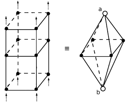
Figure 3: Wheatstone bridge (WB) hierarchical lattice obtained from a cubic lattice. It has $b=2$ and Hausdorff fractal dimension $d=\log 12/\log 2\approx 3.585$.

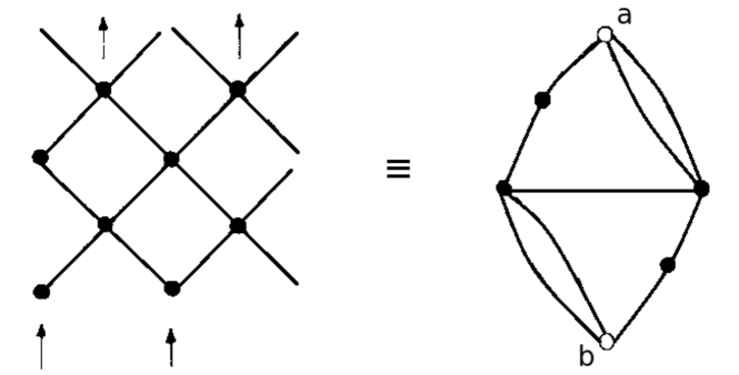
Figure 4: Left hand side: square cells of cell spacing length $b=3$. On the right side: corresponding folded square hierarchical lattices with two roots (open circles). All outcoming and incoming sites, pointed by the arrows, are put together and generate, respectively, root sites a and b. The inner sites of the square cell become the inner sites of the folded square hierarchical lattice. Note that with this construction we obtain self-dual lattices with fractal dimension $d=\ln 9/\ln 3=2$.

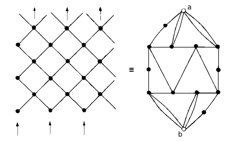
Figure 5: Folded square lattice obtained as in Fig. 4, but for $b=5$.

The above PSRG scheme holds when the coupling constants $J_{ij}$ are all equal and the external field is ordered and homogeneous. To perform the equivalent analysis of the critical behavior in disordered systems one has to generalize the PSRG method to probability distributions of interaction parameters.

3 Hierarchical renormalization in presence of quenched disorder

In disordered systems the PSRG transformation is described by the evolution of a probability distribution rather than single values of coupling constants: Harris74b ; Andelman84

$$P^{\prime}({\cal J}_{R})=\int\left[\prod_{\alpha=1}^{b^{d}}d{\cal J}_{\alpha}P({\cal J}_{\alpha})\right]\delta\left[{\cal J}_{R}-{\cal R}(\{{\cal J}\}_{b^{d}})\right]$$

(14)

where ${\cal J}$ is the set of external parameters (couplings, fields, chemical potentials, $\ldots$), $b$ is the length of the cell in lattice spacings (i.e., the scaling factor in the decimation procedure), $d$ the space dimension, so that $b^{d}$ is the size of the cell in number of bonds to be decimated, and ${\cal R}(\{{\cal J}\}_{b^{d}})$ is the local recursion relation for the interactions.

In MK lattices, because of their 1D-like topology, see, e.g., Fig. 2, the transformation can be divided into steps of so-called bond-moving and decimation, each of which involving only two bonds at a time. It is, thus, possible to exactly compute the probability distribution and represent it with histograms, each bin of which characterized by a value of the interactions and an associated probability Falicov_96 .

Figure 6: RG evolution of the probability distribution of nearest-neighbor interaction for the spin-glass Ising model on the Wheatstone bridge lattice of Fig. 3 ($D\simeq 3.58$) and pool size $M=10^{6}$. Paramagnetic (left), Ferromagnetic (center) and Spin-Glasss (right) phases.

In HLs built without the MK 1D-like structure, such as the Wheatstone-bridge-like in Fig. 1, this factorization is no longer possible and we must consider the convolution of more than two links at a time. We are, eventually, obliged to proceed in a statistical way. The PSRG scheme is, then, accomplished by representing the probability distribution of the couplings by a pool of $M$ real numbers Southern77 from which one can compute its associated moments, at each renormalization step. In the limit $M\rightarrow\infty$ these moments should approach those of the exact renormalized probability distribution. The process starts by creating a pool with $M$ coupling constants generated according to the initial distribution. A PSRG iteration consists in $M$ operations in which one randomly picks a set of $b^{d}$ couplings from the pool in order to generate one renormalized coupling, which will populate the renormalized pool. Following this procedure, one creates a new pool of size $M$ representing the renormalized probability distribution. During the PSRG procedure the moments of the coupling distribution are of particular interest for the identification of the phases.

For example, in Ising models with quenched disorder, denoting by $J$ the average of the couplings and by $\sigma_{J}$ the mean square displacement, one obtains the Paramagnetic (PM), Ferromagnetic (FM), and Spin Glass (SG) phases, as dominated by the attractors    $J\rightarrow 0;$ $\sigma_{J}\rightarrow 0;$  PM ; $J\rightarrow\infty;$ $\sigma_{J}\rightarrow\infty\;\;\left(J/\sigma_{J}\rightarrow\infty\right);$ FM ; $J\rightarrow 0;$ $\sigma_{J}\rightarrow\infty;$ SG .

In Fig. 6 the typical PSRG iterations of the couplings distribution in the three phases are shown for the random bond Ising model on the Wheatstone bridge lattice of Fig. 3.

In order to reduce the dependence on a particular sequence of random numbers, the evolution of each distribution is analyzed over $N_{S}$ different samples. This is especially relevant when the starting pool is near a critical point, and random fluctuations can lead different samples of the same distribution into different attractors. In this case we will adopt the convention that a phase is identified if at least $80\%$ of the $N_{S}$ samples flow into the same attractor. This defines the error for the location of critical points, which can be reduced by increasing the value of $M$.

In presence of disorder it is hard to devise a general prescription for finding the critical exponents, like the one provided by Eqs. (6), (LABEL:eq_der_BF) for ordered models. The idea is, then, to estimate the critical exponents by slightly perturbing the system from the unstable fixed point distribution and measure how fast it departs from it under successive PSRG iterations. We will discuss this procedure in detail in the following.

3.1 Random Field Ising Model

In this section we discuss the PSRG study of the Random Field Ising Model (RFIM) with bimodal and Gaussian distributed quenched external field on the simple necklace MK lattice of Fig. 2, with fractal dimension $d=3$, and on the Wheatstone-Bridge (WB) hierarchical lattice of Fig. 3, with fractal dimension $d\approx 3.585$ .

The initial distribution of couplings for the RFIM reads

$$P(J_{ij},h_{ij},h^{\dagger}_{ij})\!=\!\delta(J_{ij}-1)\,p(h_{ij})\,\delta(h^{\dagger}_{ij})$$ (15)

where $p(h_{ij})$ is either a bimodal or a Gaussian distribution:

$$p(h_{ij})\!=\!\left\{\begin{array}[]{l}\frac{1}{2}\left[\delta(h_{ij}\!-\!h_{0})\!+\!\delta(h_{ij}\!+\!h_{0})\right],\vspace{.3cm}\\ \frac{1}{\sqrt{2\pi h_{0}^{2}}}\exp\left\{-\frac{h_{ij}^{2}}{2h_{0}^{2}}\right\}.\end{array}\right.$$ (16)

The initial distribution is an even function of $h$, and $h^{\dagger}$. This symmetry is preserved under the PSRG transformation. To maintain this symmetry in our finite sample, we, actually, use a pool of $2M$ interactions: for each of the $M$ computed renormalized interactions $(J_{ij},h_{ij},h^{\dagger}_{ij})$ we add to the pool also the corresponding $(J_{ij},-h_{ij},-h^{\dagger}_{ij})$.

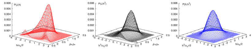
Figure 7: Projections of the critical $T=0$ fixed probability distribution for RFIM on WB $2$D lattice for bimodal initial distribution on $J,h$ (left), $J,h^{\dagger}$ (mid) and $h,h^{\dagger}$ planes.

This trick becomes important for long PSRG iterations. As $M$ increases the PSRG threshold step beyond which it becomes necessary quickly increases. This forced symmetrization is, thus, not crucial in determining critical properties but helps decreasing finite size effects for small pools. For the present computation we take pools with up to $M=10^{6}$ interactions, enough to yield statistically stable results.

The RFIM shows two phases identified by the behavior of the ratio between the average coupling

$$J=\langle J_{ij}\rangle$$ (17)

and the standard deviation of the fields

$$h_{0}^{2}=\langle h_{ij}^{2}\rangle$$ (18)

along the PSRG flow: $h_{0}/J\to\infty$ high temperature phase; $h_{0}/J\to 0$ low temperature phase; (and similarly for $h^{\dagger}$ field). At the critical point both $J$ and $h_{0}$ (as well as $\sigma_{h^{\dagger}}$) flow to infinity, confirming that the critical behavior of RFIM is controlled by a zero-temperature fix point couplings distribution.

For the MK lattice of Fig. 2 and for the WB lattice shown in Fig. 3 the critical points are reported in Tab. 1.

Lattice	$h_{0}$	$h_{0}/J$
bimod. MK	$0.942(4)$	$0.876(3)$
Gauss MK	$0.934(5)$	$0.869(4)$
bimod. WB	$0.460(3)(2)$	$0.443(5)$
Gauss WB	$0.456(3)$	$0.448(4)$

Table 1: Critical fixed points exponents for RFIM on necklace MK lattice in Fig. 2 and WB lattice in Fig. 3 with bimodal and Gaussian random field distributions.

In Fig. 7 we show the projections of the critical fix point probability distribution for the bimodal case on the WB hierarchical lattice (in the Gaussian case they are qualitatively the same).

At the zero-temperature fix point there are three independent exponents: the scaling exponent of the distribution of couplings $z$, the magnetic field scaling exponent $y_{h}$ and the thermal scaling exponent $y_{T}=1/\nu$ BM85 . They can be obtained following the procedure proposed by Cao and Machta Cao92 , for both the bimodal and Gaussian case.

Distribution growth scaling.        The exponent $z$ describes the deviation of the couplings probability distribution from the unstable fix point distribution under the PSRG transform. In order to estimate $z$, once the PSRG flux gets close to the fix point distribution, we fix the ratio $h_{0}/J$ at the critical value in the subsequent PSRG iterations by shifting at each step all the couplings $\{J_{ij}\}$ in the pool towards the ideal critical value.

In particular, we compute the average $J$ in the given iteration and we compute the $J^{*}$ that the system should display if $J^{*}=h_{0}/[h_{0}/J]_{c}$. Then we take $J^{*}-J$ and we choose to change each one of the $J_{ij}$ in the distribution of the 80% of $J^{*}-J$. In our computation each one of these shifts turns out to be very small, of the order of 0.1% for each $J_{ij}$. This is, though, an essential change because of the unstable nature of the fix point.

We, then, evaluate the rescaling factor $\lambda\equiv h_{0}^{\prime}/h_{0}\simeq J/J^{\prime}$ at each PSRG step next to the critical line and then take its average. The exponent is estimated as

$$z=\log_{b}\overline{\lambda}\,,$$ (19)

where the overbar denotes the average over $10$ PSRG steps. Its values on the MK and WB cells both with bimodal and Gaussian distribution are shown in Tab. 2. We note that in all the cases it is $z\leq d/2$, that is the upper bound provided by Berker and McKay Berker86 .

External field scaling.        The exponent $y_{h}$ describes the rescaling of an infinitesimal homogeneous field and can be obtained by averaging the relations in Eq. (6), (LABEL:eq_der_BF) over the fix point distribution

$$y_{h}=\log_{b}\left<\frac{\partial h_{R}}{\partial h}\right>\,.$$ (20)

Its values are reported in Tab. 2 for the different cases. In all cases the value is smaller than the fractal dimension $d$, which is $3$ for MK and $\sim 3.585$ for WB, implying that the magnetization is continuous at the transition.

Correlation length scaling.        In order to estimate the exponent $\nu$, we first reach a pool of renormalized couplings satisfactorily representing the fix point distribution. Next we take a copy of the pool and generate a slightly perturbed couplings probability distribution by shifting every coupling $\{J_{ij}\}$ of the replicated pool by a small amount $\delta=10^{-4}J$. The original and the perturbed pools are, then, simultaneously renormalized. To reduce statistical fluctuations the couplings in the pool representing the fix point probability distribution are shifted, after each PSRG step, to keep the distribution close to the unstable fix point, in a manner similar to that used for the estimation of the exponent $z$. Note that in this way the only role of the shift $\delta$ is to accelerate and make explicit the departure from the fixed point.

By defining $t_{n}$ as the difference between the value of the ratio $h_{0}/J$ in the two pools after $n$ PSRG iterations, the correlation length exponent is estimated as

$$\frac{1}{\nu}=\log_{b}\overline{\left(\frac{t_{n+1}}{t_{n}}\right)}\,,$$ (21)

where the overbar denotes the average over the PSRG iterations $n$. Note that the argument of the logarithm is always positive, because leaving the fix point the second copy variance can either shrink or increase in its flux, but it does not oscillates between different PSRG steps. The sign of $t_{n}$ and $t_{n+1}$ is, thus, the same.

Typically we have $n=3,\ldots,9$, for which the perturbed pool is not too far from the unstable fix point, and the ratio $h_{0}/J$ is stable. The result is independent of $M$ and it is quite stable over independent PSRG evolutions, at least for $M\gtrsim 10^{5}$.

We obtain $1/\nu=0.45\pm 0.23$ for the bimodal distribution and $1/\nu=0.44\pm 0.20$ for the Gaussian distribution on the MK lattice. Similarly, for the WB lattice we find $1/\nu=0.69\pm 0.35$ for the bimodal distribution and $1/\nu=0.68\pm 0.31$ for the gaussian distribution. As summerized in Table  2. Once the exponents $z$, $y_{h}$ and $\nu$ are known, the exponents $\alpha$ and $\beta$ are obtained from the scaling relations BM85

$$\alpha = 2-(d-z)\nu,$$ (22)

$$\beta = (d-y_{h})\nu.$$ (23)

Notice that, at difference with Eq. (9-13), here the fixed point is at zero $T$ (as $1/J$) and the index $z\neq 0$.

The critical exponents obtained on MK lattice for the bimodal case are compatible with those obtained by Cao and Machta Cao92 . The exponents $y_{h}$ and $z$ depend strongly on the fractal dimension of the lattice, and their value for the $d=3$ MK lattice are in good agreement with the results for the three dimensional Bravais lattice, whilst for the $d\simeq 3.585$ WB lattice they are closer to that found for the four dimensional Bravais lattice, cf. Table 2.

The value of the exponent $\nu$ is larger for the WB hierarchical lattice than for the MK lattice, as in agreement with the behavior in hyper-cubic lattices of increasing dimensions. Although the error bars for this exponent are large, we stress that in this case only the WB lattice gives a numerical estimate compatible with the result for the cubic lattice.

We, eventually, notice that the Gaussian and bimodal exponents are always compatible with each other and belong to the same universality class.

Lattice	$z$	$y_{h}$	$1/\nu$
bimod. MK	$1.491(3)$	$2.991(1)$	$0.45(23)$
bimod. MK Falicov95	$1.4916(3)$	$2.9911(2)$	$0.445(2)$
Gauss MK	$1.486(3)$	$2.990(1)$	$0.44(20)$
bimod. WB	$1.788(2)$	$3.575(1)$	$0.69(35)$
Gauss WB	$1.787(2)$	$3.576(1)$	$0.68(31)$
3d MC Sim_RFIM	$1.49(3)$	$2.988(4)$	$0.73(5)$
4d MC SIM_RFIM_4d	$1.779(4)$	$3.827(1)$	$1.280(2)$

Table 2: Critical exponents at critical fixed distribution for RFIM on necklace MK lattice in Fig. 2 and WB lattice in Fig. 3. The last two rows relate to simulations on Bravais 3D and 4D hyper-cubic lattices with bimodal distributed interactions. The more accurate exponents in Ref. Falicov95 are obtained using the histograms representation for the interactions probability distribution, that is a feasible method only for MK cells.

In the RFIM the bond are at first all equal, and the disorder is on site. The major reason of moving from MK lattices to more complex HL is, actually, the need of a better treatment of the bond structure. In the next sections we move to models in which the disorder is on the bond from the outset.

3.2 Random Bond Ising model in $d\leq 2.5$

In this Section we consider the Ising model with bimodal $\pm J$ bond distribution on hierarchical lattices mimicking the topology of the square lattice.

The initial probability distribution for interactions is

$$P(J_{ij},h_{ij},h^{\dagger}_{ij}) = \left[p\delta(J_{ij}-J)+(1-p)\delta(J_{ij}+J)\right]\,\delta\left(h_{ij}\right)\delta\left(h^{\dagger}_{ij}\right)$$ (24)

where $J>0$ and $p\in[0,1]$ is the probability of a ferromagnetic bond.

For low enough $p$, this model on regular lattice has an antiferromagnetic phase. On hierarchical lattices the antiferromagnetic order is preserved under PSRG only when the rescaling factor $b$ is odd, so that a symmetric phase diagram in $p\leftrightarrow(1-p)$ is obtained, where the ferromagnetic phase is replaced by the antiferromagnetic phase and vice-versa.

To capture some features of Bravais lattices, we shall focus on hierarchical lattices with elementary cell more complex than the $1$D-like MK cells. In particular we shall consider the cell proposed by Nobre Nobre01 , Fig. 4, with rescaling factor $b=3$ and its extension to $b=5$, Fig. 5.

Nishimori conjecture.  Even though the Random Bond Ising model in 2D does not display any spin-glass phase Ohzeki09 , this model on hierarchical lattices is an excellent play ground to test Nishimori’s conjecture Nishimori01 ; Nishimori02 . Here we briefly recall what the conjecture is.

The idea behind it stems from noting that the partition function $\mathcal{Z}$ of non-random Ising models on self-dual lattices is itself self-dual Wegner .

Let us express $\mathcal{Z}$ in terms of the edge Boltzmann factors $u_{\pm 1}(J)=e^{\pm J}$ (note the use of the reduced parameters). The Fourier transform of $u_{\pm 1}(J)$, $u^{*}_{\pm 1}(J)$, is the dual Boltzmann factor Wu_Wang . As a consequence, the critical point of a self-dual model is obtained by the fix point condition $u_{\pm 1}(J)=u_{\pm 1}^{*}(J)$, which yields $J_{c}=\frac{1}{2}\log(\sqrt{2}+1)$.

Within the replica method approach, the relevant variables are the averaged edge Boltzmann factors $x_{k}(p,J)$, which correspond to the configuration with the spin connected by the bond equal to +1 in $n-k$ replicas and $-1$ in remaining $k$ replicas. Self-duality is now expressed by the invariance of $\mathcal{Z}_{n}\equiv\overline{\mathcal{Z}^{n}}$ under the simultaneous exchange $x_{k}(p,J)\leftrightarrow x^{*}_{k}(p,J)$ for all $k$. The overbar denotes the average over quenched bond disorder. Unlike the non-random case, it is not possible to identify the critical point from the fix point condition of the duality relations, because the relations with $k=0,\ldots,n$ are not satisfied simultaneously. The Nishimori’s conjecture Maillard03 ; Takeda , then, identifies a point $(p_{N},J_{N})$, called ”multicritical”, by means of a fix point condition for the leading $k=0$ Boltzmann factor

$$x_{0}(p_{N},J_{N})=x^{*}_{0}(p_{N},J_{N})\,,$$ (25)

on the Nishimori line $e^{-2J}=(1-p)/p$,Nishimori81 ; Nishimori01 where enhanced symmetry simplifies the system properties significantly. This point of the Nishimori line is called multicritical because, when a SG phase is present, it is the point at which PM, FM and SG phases are all in contact with each other. This does not occurs in 2D, see, e.g., Fig. 8 but it does occur in 3D, cf. Fig. 13.

The conjecture is proved exact for $n=1,2$ and $\infty$. In the limit $n\to 0$ the condition $x_{0}=x^{*}_{0}$ on the Nishimori line becomes

$$H(p_{N})\equiv-p_{N}\log_{2}(p_{N})-(1-p_{N})\log_{2}(1-p_{N})=\frac{1}{2}\,,$$ (26)

where the function $H(p_{N})$ is the binary entropy.

This conjecture turns out to be wrong for some systems on HL.Hinczewski05 ; Ohzeki08 Ohzeki, Nishimori and Berker Ohzeki08 ; Nishimori10 noted that for HL’s a systematic approximation for the multicritical point can be obtained by imposing Eq. (25) at each PSRG transformations.

Note that in the two-dimensional case, even though the SG phase is absent, the Nishimori point is expected to coincide with a critical point, unstable along the phase boundary; so, as it is usually done, in the following we identify the Nishimori point as the intersection between the Nishimori and the critical lines.

Here we test the original Nishimori conjecture on a Folded Square (FS) hierarchical lattice constructed through a bond-moving procedure that, at difference with the MK bond-moving prescription, retains the local correlation of the bonds, see Figs. 4 and 5.

3.2.1 Numerical results

In Fig. 8 we show the $p,T(=1/J)$ phase diagram obtained from the PSRG analysis in two dimensions on the lattice shown in Fig. 5 with rescaling factor $b=5$.

For $p=1$ we find the critical temperature is $T_{c}=2.269185(1)$, in agreement with the Onsager solution $T_{c}=2/\log(1+\sqrt{2})\simeq 2.269185$. This result, also found for the folded square lattice of Fig. 4 with $b=3$,Nobre01 and WB with $d=2.32$, Salmon10 follows from the duality properties of the unit cells.Tsallis_96

Nishimori point.   The position of the multi-critical point expected from Nishimori’s conjecture, Eq. (26), is $p_{N}\simeq 0.889972$. For the cell of Fig. 4 the estimated value is $p_{N}=0.8903(2)$ $(2H(p_{N})=0.998(1))$Ohzeki08 with $T_{N}=0.9557(18)$.Nobre01

For the cell of Fig. 5, performing $N_{S}=20$ independent PSRG calculations with a poll of $M=10^{5}$ initial bond configurations, we estimate (cf. Table 3)

$$p_{N} = 0.8902(1),\quad T_{N}=0.9571(1)$$

$$2H(p_{N}) = 0.9985(1)\,;$$

yielding no difference with respect to the cell with $b=3$. We conclude that the conjecture fails also on this more complex hierarchical lattice.

The folded square cell estimates with $b=3$ or $b=5$ turn out to be in good agreement with each other and with the estimate $p_{N}=0.8905(5)$ given by the transfer matrix approach, Reis99 but are slightly larger than those from high temperature series expansion, $p_{N}=0.886(3)$, Singh96 and Monte Carlo simulation, $p_{N}=0.8872(8)$. Ozeki98

In Table 3 we report the results on critical points for an easier comparison.

Critical slope.        A quantity usually studied is the slope of the critical line close to $p=1$:Harris74

$$s\equiv{\frac{1}{T_{c}(1)}}{{\frac{dT_{c}(p)}{dp}}\bigg{|}_{p=1}}\,.$$ (27)

The Domany’s perturbative approach Domany79 yields $s=2\sqrt{2}/[\ln(\sqrt{2}+1)]\simeq 3.209$ for the Ising with $\pm J$ bond distribution on square lattice. The approach assumes weak disorder, i.e., a qualitatively irrelevant disorder that does not undermine the existence of the ferromagnetic phase at low $T$ and does not change the universality class of the PM/FM transition for $p<1$. By computing $s$ it is, thus, argued that one can discriminate whether quenched disorder is a relevant perturbation, causing a change in the universality class. Ohzeki11 Ohzeki and collaborators Ohzeki11 suggest that Domany’s method can be applied to any self-dual lattice, and then one can probe the relevance of disorder from the slope $s$ also for the HL of Figs. 4 and 5.

The duality approach gives $s=3.27866...$ Ohzeki11 for the lattice in Fig. 4 with $b=3$. From a best fit of the points close to $p=1$ with a pool of size $M=5\cdot 10^{6}$ with $N_{S}=20$ samples we obtain $s=3.30(3)$, compatible with, though less precise than, the duality estimate. In the $b=5$ case of Fig. 5, with a pool of size $M=5\cdot 10^{6}$ with $N_{S}=20$ samples we find $s=3.32(3)$. Both values are different from Domany’s prediction $s\simeq 3.209$.Domany79 This is not, however, a strong issue in favor of strong disorder.

According to the argument of Ref. Ohzeki11 this would imply that the disorder should be relevant in these cases. However, if it is true that a slope equal to Domany’s slope might be consistent with the hypothesis of irrelevant disorder, the fact that the slope is different from Domany’s value does not, actually, imply the opposite (i.e., the existence of a new ”strong disorder” fixed point). Indeed, the HL RG approach already fails to quantitatively precisely capture the critical behavior of the system and the lack of a numerical coincidence is just a consequence of this. One can confirm this by direct inspection, yielding no other fix points after disorder is introduced and, consequently, no universality class change. Any coupling distribution on the transition line tends to become more and more peaked under PSRG transformations, tending to the pure FM-PM critical fixed point, as shown in Fig. 9. Disorder in the two dimensional Ising model does not appear to play any role on any lattice cell analyzed here (see also the Harris criterion below).

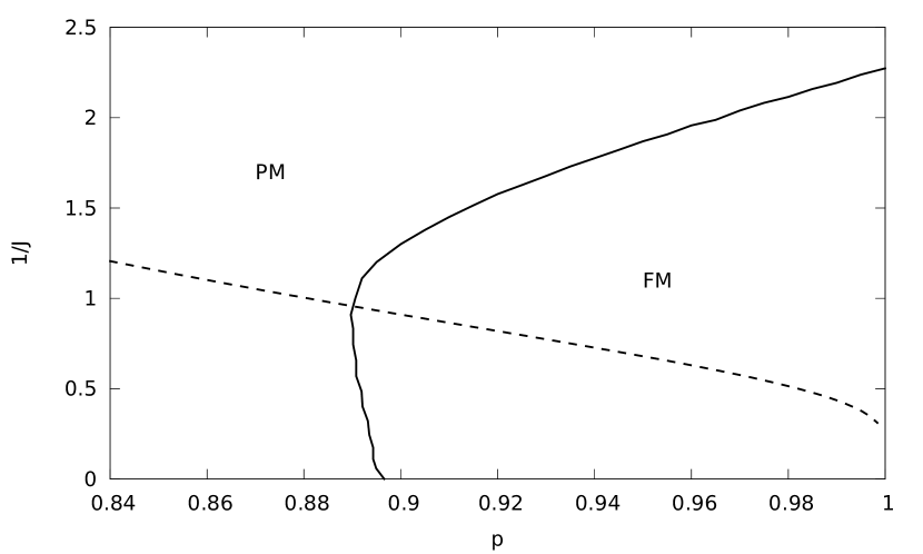
Figure 8: Phase diagram of Ising 2D with “folded square” HL with $b=5$. The diagram is symmetric in $p\rightarrow 1-p$ and the anti-ferromagnetic part is not shown. The dashed line represents the Nishimori line.

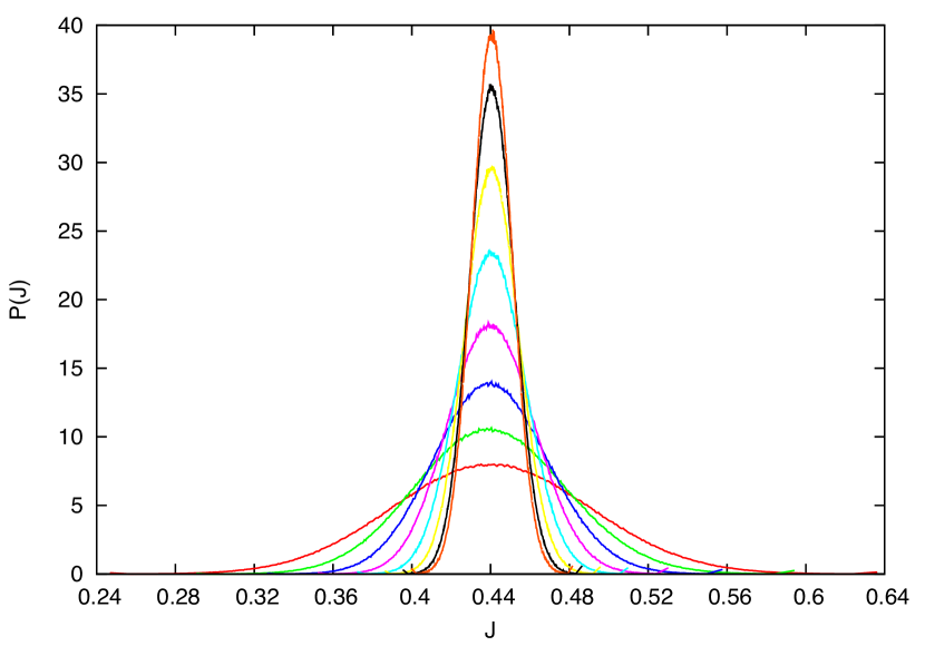
Figure 9: PSRG evolution of the coupling distribution on the critical line near the pure fixed point (steps from 4 to 11 are shown for $p=0.01$): the width quickly decreases, so that the distribution tends to a Dirac delta and the disorder disappears. No other fixed distribution. besides the pure criticality, are obtained on the PM-FM transition line.

HL / Method	Fig./Ref.	$p_{N}$	$p_{T=0}$
FS $b=3$	4/Nobre01	$0.8903(2)$	$0.8951(3)$
FS $b=5$	5	$0.8902(1)$	$0.8966(2)$
	Reis99	$0.8905(5)$
Square	Singh96	$0.886(3)$
	Ozeki98	$0.8872(8)$
	Kawashima97		$0.896(1)$
	Kawashima97		$0.894(2)$
Nishimori conjecture	Nishimori01	$0.889972...$

Table 3: Multicritical point as computed on different HLs and different estimates on the square lattice.

Harris criterion.  The widely accepted form of the Harris criterion Harris74 ; Chayes is that in ferromagnetic systems with random interactions the randomness is irrelevant if $\alpha$, the specific heat exponent of the corresponding pure system, is negative, while for systems with positive $\alpha$ the random system exhibits different critical behavior in presence of disorder. For the folded square lattices for both $b=3$ and $b=5$ we find $\alpha<0$.

Though it is known that this criterion can fail on HL if the bonds in the rescaling volume are not all equivalent,Andelman84 ; Kinzel81 ; Andelman85 ; Derrida ; Sutapa ; Efrat in the present case the Harris criterion is, actually, satisfied since the disorder is irrelevant, as discussed above with respect to the critical slope value.

FM line reentrance.   An important feature of the $p,T$ diagram, according to the duality requirements, is the reentrance of the transition line below the multicritical point: $p_{N}>p_{T=0}$. The zero temperature transition point $p_{T=0}$ can be estimated by finite size scaling analyses of the ground state. Calling $E_{p}$ and $E_{a}$ the ground-state energies with, respectively, periodic and anti-periodic boundary conditions in one direction, and $\Delta=E_{p}-E_{a}$ the domain wall energy, we can determine two estimates of critical concentrations of antiferromagnetic bonds by looking at the point where the asymptotic dependences $[\Delta]$ and $[\Delta^{2}]^{1/2}$ change from increasing to decreasing, where the average $[\ldots]$ is taken on different bond samples. More explicitly, by defining

$$[\Delta]\sim L^{\rho}\quad\text{and}\quad[\Delta^{2}]^{1/2}\sim L^{\theta}\,,$$ (28)

via the determination of exact ground states for large system sizes and huge sample numbers, Kawashima and Rieger give the estimates $p_{T=0}^{(\rho)}=0.896(1)$ and $p_{T=0}^{(\theta)}=0.894(2)$ looking at the point where $\rho$ and $\theta$ respectively change sign Kawashima97 . The PSRG approach with the folded square of Fig. 4 ($b=3$) leads to $p_{T=0}=0.8951(3)$ Nobre01 , while with the cell of Fig. 5 ($b=5$) we find $p_{T=0}=0.8966(2)$ as summarized in Tab. 2.

The critical indices for the pure ferromagnetic point can be evaluated as discussed in Sec. 2.1: we obtain $y_{T}=0.7303(1)$ and $y_{h}=0.8518(1)$ for the folded square lattice with $b=3$ and for the folded square lattice with $b=5$ we find $y_{T}=0.7589(1)$ and $y_{h}=1.059(1)$. In both cases they are not consistent with the values of Onsager solution, which read $y_{T}=1$ and $y_{h}=1.875$, respectively. From the knowledge of $y_{T}$ and $y_{h}$ the critical indexes are obtained from the usual scaling relations, cf. Eq. (13) and their numerical values are reported and compared on Table 4.

Zero temperature stiffness.  We conclude this section by discussing the exponent $\nu$ of the zero-temperature spin-glass transition for the case of a Gaussian distribution of bonds with zero mean and initial width $\sigma_{J}$. It can be obtained directly from scaling of $\sigma_{J}$ under PSRG :

$$\sigma^{\prime}_{J}(b)\sim\sigma_{J}b^{\theta}.$$ (29)

The sign of the stiffness exponent $\theta$ is directly related to the low temperature phase: for positive (negative) $\theta$ the system scales under PSRG flow towards strong (weak) couplings, distinctive of a low temperature spin-glass (high $T$ paramagnetic) phase. For continuous and symmetric probability distributions $P(J)$, the temperature $T$ appears in the PSRG equations as a dimensionless ratio between couplings, so that the scaling (29) is equivalent to $T\sim L^{\theta}$, or $L\sim T^{1/\theta}$. In a phase transition at $T\rightarrow 0$ the latter scaling can be identified with the scaling of the correlation length $\xi\sim T^{-\nu}$ implying Bray84 :

$$\nu=-\frac{1}{\theta}.$$ (30)

	FS b=3	FS b=5	Exact
$\alpha$	-0.7385(1)	-0.6353(1)	0
$\beta$	1.572(1)	1.240(1)	0.125
$\gamma$	-0.4057(1)	0.1558(1)	1.75
$\delta$	0.7419(1)	1.126(1)	15
$\nu$	1.369(1)	1.318(1)	1
$\eta$	2.296(1)	1.882(1)	0.25

Table 4: Critical indices of pure ferromagnetic critical point for Ising model on the folded square lattice for $b=3$, Fig. 4, and for $b=5$, Fig. 5.

Lattice type	Fig.	Ref.	$\theta$
MK $b=2$		Southern77 ]	$-0.270(2)$
MK $b=3$		Nobre98	$-0.278(2)$
WB $b=2$	1	Tsallis_96	$-0.290(3)$
WB $b=3$		Nobre98	$-0.298(2)$
FS $b=3$	4	Tsallis_96	$-0.275(1)$
FS $b=5$	5		$-0.2714(2)$
		Bray87	$-0.291(2)$
Square		Bray02	$-0.287(4)$
		Weigel07	$-0.284(4)$

Table 5: Stiffness exponent $\theta$ on different HLs and different estimates on the square lattice.

In Fig. 10 the behavior of $\sigma_{J}$ is shown as function of PSRG steps for the case of zero-average Gaussian initial bond distribution on the folded square cell of Fig. 5. From this we get $\theta=-0.2714(2)$, leading to $\nu=3.685(3)$. For the cell of Fig. 4, with $b=3$ it was found $\theta=-0.275(1)$ Nobre98 . We report in Table 5 the values obtained on different HLs Southern77 ; Tsallis_96 ; Nobre98 ; Salmon10 and on the square Bravais lattice Bray87 ; Bray02 ; Weigel07 . For the folded square with both $b=3$ or $b=5$ the value is similar to that found for the MK lattice, whilst for the WB lattices the values are closer to that of the regular lattice, especially the case with $b=2$.

As a general remark, from Table 4 we observe that in passing from $b=3$ to $b=5$, and thus increasing the connectivity of the lattice, for the pure model we obtain a slight improvement for all exponents towards the exact values of the square lattice, though the values are very far from the exact ones. A possible convergence is, thus, so slow that the degree of inner correlation of a folded cell of a HL necessary to reproduce 2D RG might be so large to make a single cell comparable with a whole real Bravais lattices.

We now move to models in which there is a spin-glass phase, in order to test the critical behavior prediction of HL RG in the case of strong disorder.

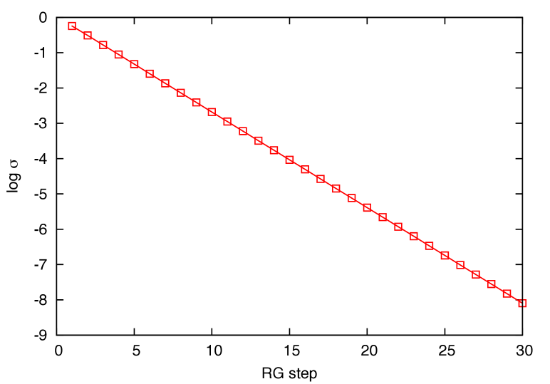
Figure 10: Standard deviation of the Gaussian probability distribution of quenched disorder at $T=0$ vs PSRG iteration steps .

3.3 Random bond Ising model in $d\geq 3$

In this section we consider the Ising model with the $\pm J$ coupling distribution, Eq. (24) on hierarchical lattices mimicking the topology of the cubic lattice. Recently, Salmon, Agostini and Nobre have studied the Ising spin glass on the hierarchical Wheatstone bridge (WB) lattices Salmon10 , obtaining accurate phase diagrams and showing that on these lattices the lower critical dimension for the spin glass phase is greater than $d=\ln 5/\ln 2\simeq 2.32$, cf. the WB HL in Fig. 1. The next pattern of the WB family, cf. Fig. 3, corresponding to a lattice in dimension higher than $2.5$ has a fractal dimension $d\approx 3.58$. Consistent quantitive deviations from the cubic lattice behavior might, then, occur.

We, here, investigate the model on the Folded Cube (FC) hierarchical lattice shown in Fig. 11. This is the ”three-dimensional” extension of the folded square lattice of Fig. 4, and it was introduced to study the anisotropic ferromagnetic Potts model in three dimensions Tsallis84 . This lattice has a fractal dimension $d=\ln 35/\ln 3\simeq 3.2362$, always larger than $3$, though nearer to it as compared to the WB. It has $b=3$ and, unlike the latter, it is able to retain a possible antiferromagnetic order, as well. As a further comparison we will report on the critical properties of the Ising spin-glass model on a MK lattice with $b=3$ and fractal dimension $d=3$, cf. Fig. 12, introduced in Refs. Erbas05 ; Ozcelik08 .

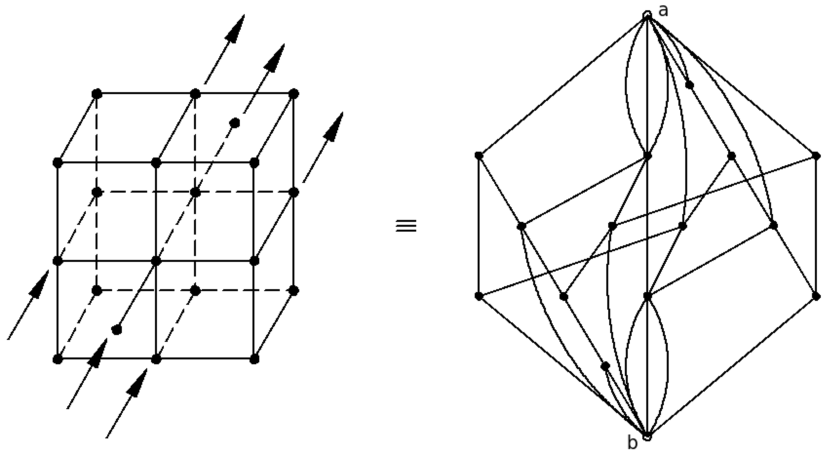
Figure 11: Cubic cells of length $b=3$ on the left hand side, and relative folded cube hierarchical lattice on the right hand side. The two roots are open circles. All incoming sites and all outcoming ones, pointed by the arrows in the left figure, are put together and generate root sites a and b on the right hand side figure. The inner sites of the cubic cell become the inner sites of the hierarchical cell.

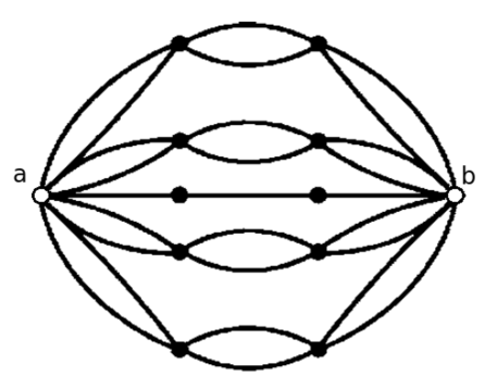
Figure 12: MK lattice with $b=d=3$.Erbas05 ; Hinczewski05

Figure 13: Phase diagram of Ising spin glass model on the Folded Cube HL, cf. Fig. 11, obtained for $M=5\cdot 10^{4}$ and $N_{S}=10$. The dashed line represents the Nishimori line. The plot is symmetric in $p\to 1-p$ and an antiferromagnetic phase is present a small $p$, in place of the FM one.

The resulting phase diagram is shown in Fig. 13. An important feature of the phase diagram is the small reentrance in the region below the multicritical point. As a consequence, by lowering the temperature one can go from the high temperature (disordered) paramagnetic (PM) phase to an ordered ferromagnetic (FM) phase and, eventually to a low temperature disordered spin-glass (SG) phase. The values of the critical points are reported in Table  6.

	.  $\begin{array}[]{c}p\\ T\end{array}$	fixed	points	coordinates   .

HL	FM	SG	$T=0$	MC
$\begin{array}[]{c}\mbox{Fold cube}\\ \mbox{ Fig. \ref{Tsallis_3d} }\end{array}$	$\begin{array}[]{c}1\\ 5.066(1)\end{array}$	$\begin{array}[]{c}0.5\\ 1.072(1)\end{array}$	$\begin{array}[]{c}0.764(2)\\ 0\end{array}$	$\begin{array}[]{c}0.7547(3)\\ 1.779(1)\end{array}$
$\begin{array}[]{c}\mbox{ WB ``3D"}\\ \mbox{ Fig. \ref{WB_lattice} }\end{array}$	$\begin{array}[]{c}1\\ 5.457(1)\end{array}$	$\begin{array}[]{c}0.5\\ 1.112(2)\end{array}$	$\begin{array}[]{c}0.760(1)\\ 0\end{array}$	$\begin{array}[]{c}0.745(2)\\ 1.620(2)\end{array}$
$\begin{array}[]{c}\mbox{ WB ``4D"}\\ \mbox{ Ref. \cite[cite]{\@@bibref{Authors Phrase1YearPhrase2}{Salmon10}{\@@citephrase{(}}{\@@citephrase{)}}} }\end{array}$		$\begin{array}[]{c}0.5\\ 2.515(2)\end{array}$	$\begin{array}[]{c}0.667(2)\\ 0\end{array}$	$\begin{array}[]{c}0.664(2)\\ 2.836(2)\end{array}$
$\begin{array}[]{c}\mbox{ MK}\\ \mbox{Fig. \ref{reticolo_MK_3d} }\end{array}$	$\begin{array}[]{c}1\\ 5.383(1)\end{array}$	$\begin{array}[]{c}0.5\\ 1.136(4)\end{array}$	$\begin{array}[]{c}0.761(1)\\ 0\end{array}$	$\begin{array}[]{c}0.752(7)\\ 1.797(3)\end{array}$

Table 6: Position of typical critical points of phase diagram in Fig. 13 for the hierarchical lattice 11: ferromagnetic (FM), spin-glass (SG), zero temperature ($T=0$) and multi critical point (MC). For comparison also values of the same fixed points are reported for other hierarchical lattices discussed in the text.

3.3.1 FM fixed point

The transition at $p=1$ on the folded cube cell is obtained at $T_{c}=5.066(1)$, $12\%$ larger as compared to the same model on cubic lattice (where $T_{c}=4.5115...$ Talapov96 ). On the $d\simeq 3.58$ WB lattice the difference was about $21\%$. Salmon10 On the MK lattices the best known result is obtained for the $d=3$ lattice in Fig. 12, where the critical temperature of the pure transition is $T_{c}=5.38(3)$, $19\%$ larger than the one in the cubic lattice. Erbas05

In the folded cube the points on the critical line between the FM and the PM phases are attracted to a single fix point located at $p=1$. The critical exponents at this point are $y_{T}=1.523(1)$ and $y_{h}=1.864(1)$, identifying a second order transition Nienhuis77 . On other HLs we obtain: $y_{T}=1.149(1)$ and $y_{h}=0.9636(1)$ for the WB lattice in Fig. 3; $y_{T}=1.460(1)$ and $y_{h}=1.613(1)$ for the MK lattice in Fig. 12. These are to be compared with numerical estimates by means of simulations on the cubic lattice: $y_{T}=1.587(1)$ and $y_{h}=2.482(1)$ Pelissetto02 . None of them agrees with the cubic lattice results, even though the FC lattice in Fig. 11 yields the nearest estimate for both exponents. The corresponding physical exponents are reported in Table 7. Note, in particular, that for all the HLs considered here we have $\alpha<0$. According to the Harris criterion Harris74 this would imply that disorder is irrelevant in modifying the ferromagnetic critical behavior, whereas for all these HL’s one finds a frozen phase different from the ferromagnetic one in a given interval of $p$ values at low temperature: besides the ”weak disorder” ferromagnetic fixed point a second “strong disorder” spin-glass fixed point arises in presence of quenched randomness.

critical	MK	WB	Folded cube	Cubic
index	Fig. 12	Fig. 3	Fig. 11	Ref. Pelissetto02
$\alpha$	$-0.2169(1)$	$-1.121(1)$	$-0.1253(1)$	$0.110(1)$
$\beta$	$1.112(1)$	$2.282(1)$	$0.9012(1)$	$0.3265(3)$
$\gamma$	$-0.006490(1)$	$-1.443(1)$	$0.3229(1)$	$1.2372(5)$
$\delta$	$0.9942(1)$	$0.3676(1)$	$1.358(1)$	$4.789(2)$
$\nu$	$0.6850(1)$	$0.8705(1)$	$0.6567(1)$	$0.6301(4)$
$\eta$	$2.009(1)$	$3.658(1)$	$1.508(1)$	$0.0364(5)$

Table 7: Critical exponents in pure ferromagnetic critical point for Ising model on the folded cubic cell and comparison.

3.3.2 Spin-glass fixed point

For the FC HL in the totally disordered case $p=0.5$ the PM-SG transition is located at $T_{c}=1.072(1)$, with a difference of $4.5\%$ relatively to the Bravais cubic lattice critical point, for which the Monte Carlo simulations provide $T_{c}=1.120(4)$ Montecarlo_3d . As reported in Table 6 the WB lattice in Fig. 3 has $T_{c}=1.112(2)$ and the MK lattice in Fig. 12 has $T_{c}=1.136(4)$.

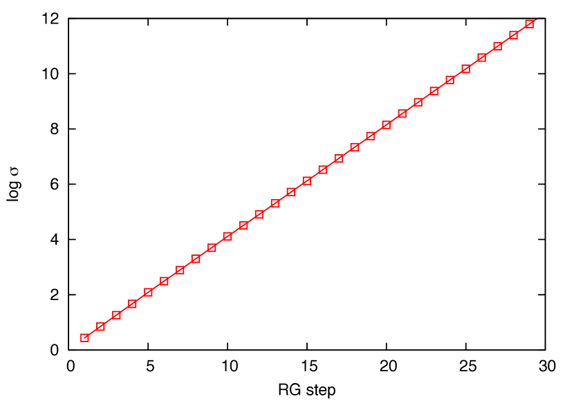
Figure 14: Graph of $\ln(\sigma_{J})$ under repeated applications of the PSRG transformation at zero temperature and $p=0.5$ on lattice in Fig. 11.

The behavior of $\ln(\sigma_{J})$ under successive PSRG iterations for $p=0.5$ is shown in Fig. 14. From its linear behavior we estimate for the stiffness exponent of the spin-glass phase $\theta=0.2052(1)$ (cf. Sec. 3.2.1). For the cubic lattice one finds in the literature $\theta=0.19(1)$ Bray87 or $\theta=0.20(5)$ Katzgraber2008 . We, thus, obtain a result very close to that expected for the cubic lattice. On the WB lattice one has $\theta=0.297(3)$ Salmon10 , while for the MK lattice it is found $\theta\approx 0.27$. Katzgraber2008 The result are summarized in Table 8.

Lattice type	Fig.	Ref.	$\theta$
MK $d=3$	12	Katzgraber2008	$0.27(1)$
WB $d\sim 3.58$	3	Salmon10	$0.297(3)$
FC $d\sim 3.24$	11		$0.2052(1)$
Cubic		Bray87	$0.19(1)$
Cubic		Katzgraber2008	$0.20(5)$

Table 8: Stiffness exponent as computed on different HL and different estimates on the cubic lattice.

All critical points along the PM-SG transition are attracted by an unstable fixed point at $p=0.5$. In Fig. 15 we show the unstable fix point coupling distributions for the three lattices considered so far. Critical exponents for this fix distribution are computed by adapting the methods used for the RFIM in Sec. 3.1. A first exponent $y_{h}$ can be obtained generalizing the pure case definition: $\lambda_{h}=\langle\partial_{h}h_{R}\rangle$, where the average is carried out by extracting the interactions from the fix point distribution. Indeed, in our case this is easy and can be exactly calculated. In fact for the fix point distribution we have $h=h^{\dagger}=0$, and so $\mathcal{H}(s)=\mathcal{H}(-s)$. It is, then, straightforward to obtain, using Eqs. (6) and (LABEL:eq_der_BF) that $\partial_{h}h_{R}=c$ for every choice of the $J$ interactions, where $c$ is the number of internal sites connected to each external site: $c=9$ for the folded cube cell in Fig. 11 and the MK in Fig. 12, $c=4$ for the WB in Fig. 3. For all these cells the exponent $y_{h}$ is then $y_{h}=\log_{b}\langle\partial_{h}h_{R}\rangle=2$ (see Sec. 2.1). We note that $y_{h}<d$, ensuring that the magnetization is continuous at the transition (no first order transition).

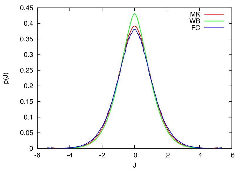
Figure 15: Fixed probability distribution for the spin glass - paramagnet transition for Ising spin glass on lattice in Fig. 12 (MK), Fig. 3 (WB) and Fig. 11 (FC). These distributions are reached after about $2-3$ steps of renormalization, starting from the binomial distribution, and maintain this shape for about $10-15$ steps steps, after which they starting moving away because of statistical fluctuations.

To get the correlation length exponent $\nu$ we note that defining $t\equiv\sigma_{J}-\sigma_{J}^{*}$, where $\sigma_{J}^{*}$ is the value at the critical point, we obtain the scaling law

$$\xi(t)=b~{}\xi(t^{\prime})=b~{}\xi(b^{x}t)=b^{n}\xi(b^{nx}t).$$ (31)

By taking $n$ such that $b^{nx}t=t_{0}$, where $t_{0}$ is arbitrary but fixed, we end up with

$$\xi(t)=\biggl{(}\frac{t_{0}}{t}\biggl{)}^{\frac{1}{x}}\xi(t_{0})\sim t^{-\frac{1}{x}},$$ (32)

from which we get $\nu=1/x$: the value of $\nu$ can be estimated by the trend of $\sigma_{J}$ near the critical point distribution.

We use the method already exposed in Sec. 3.1: after obtaining an instance of the fixed distribution, we make a copy of it and multiply each coupling of the copy by a quantity $1+\delta$, with $\delta\approx 0.05$. The two copies of the distribution are, then, simultaneously iterated in the PSRG transformation, with the first copy forced near the fixed point and the second one free to flow. We eventually estimate $\nu$ by means of Eq. (21), where the parameter $t_{n}$ is now the difference between the values of $\sigma_{J}$ in the two copies at RG step $n$.

Continuing this way we find the values shown in Table 9 for different HLs and we notice that they are compatible with each other within the statistical error. However, when compared to the estimate for the cubic Bravais lattice, none of them is compatible with it: $\nu=2.45(15)\rightarrow 1/\nu=0.408(25)$ Pelissetto08 . On top of that, we observe that quantitatively, the FC cell, of fractal dimension $3.24$ has a value of $\nu$ further away than the value on the MK and WB ones. This is a strong signature of the limitations of the RG approach on HL’s to the critical behavior of systems on Bravais lattices in presence of disorder.

Proceeding as for the correlation length, and using the free energy $f$ scaling law

$$f(t)=b^{-d}f(t^{\prime})=b^{-d}f(b^{x}t)=b^{-nd}f(b^{nx}t)$$

with $n$ such that $b^{nx}t=t_{0}$ and $t_{0}$ arbitrary but fixed, we have

$$f(t)=\biggl{(}\frac{t_{J}}{t_{0}}\biggl{)}^{\frac{d}{x}}f(t_{0})\sim t^{\frac{d}{x}}.$$ (33)

Then from $\partial^{2}f/\partial t^{2}\sim|t|^{-\alpha}$, we obtain the scaling relation

$$\alpha=2-\frac{d}{x}=2-d\nu,$$ (34)

as well as

$$\beta = \frac{\nu(1+\eta)}{2}\,,$$

$$\gamma = (2-\eta)\nu\,,$$

where

$$\eta=d+2-2y_{h}=d-2\,$$

since $y_{h}=2$ for all our HLs. The estimates of the physical exponents are reported in Table 10.

Lattice	Fig.	Resc.	Dim.	$1/\nu$
MK	12	$b=3$	$d=3$	$0.297\pm 0.026$
WB	3	$b=2$	$d\sim 3.58$	$0.308\pm 0.063$
Folded cube	11	$b=3$	$d\sim 3.24$	$0.262\pm 0.037$
Bravais cubic Pelissetto08			$d=3$	$0.408\pm 0.025$

Table 9: Estimates for the exponent $\nu$ at transition SG-para for the Ising spin glass model.

critical	MK	WB	Folded cube	Cubic
index	Fig. 12	Fig. 3	Fig. 11	Ref. Pelissetto08
$\alpha$	$-8.10(88)$	$-9.6(24)$	$-10.4(17)$	$-5.4(5)$
$\beta$	$3.37(30)$	$4.20(86)$	$4.27(60)$	$0.77(5)$
$\gamma$	$3.37(30)$	$1.35(28)$	$2.92(41)$	$5.8(4)$
$\nu$	$3.37(30)$	$3.25(66)$	$3.82(54)$	$2.45(15)$
$\eta$	$1$	$1.585\ldots$	$1.236\ldots$	$-0.375(10)$

Table 10: Estimates for the physical exponents at the SG-PM transition for the Ising spin glass model. The exponent $\eta$ is $d-2$, $d$ being the fractal dimension of the HL.

Concluding this section, on the FC lattice in Fig. 11 the estimates for the pure criticality are much closer to those on cubic lattice (although still not compatible), compared to MK in Fig. 12 and WB in Fig. 3. Also for the stiffness exponent of SG phase a remarkable improvement is observed: its estimate is compatible with its cubic value on the FC lattice but not on other HLs. For other quantities, though, at the disordered fixed point such improvement is unseen. In particular, in the estimate for the $\nu$ exponent at the SG-PM transition.

We can argue that the stiffness exponent depends more on the local geometrical properties of the lattice, that are substantially improves in the folded cube lattice, while critical properties depend on longer distances, that are still dominated by the hierarchical backbone an thus far from the Bravais lattice behavior.

More stringent tests can be obtained for the Blume-Emery-Griffiths model, that we will analyze in the next section. For this system the inverse first order transition expected from mean-field theory Crisanti05b and simulation in finite dimension Paoluzzi10 is absent on the MK lattice in Fig. 12. Ozcelik08

4 Blume-Emery-Griffiths model

We now move on to a different system, the Blume-Emery-Griffiths (BEG) model, originally devised to study the superfluidity transition and phase separation in He³-He⁴ mixtures Blume71 . The model is known to display, besides a second order phase transition, also a first order transition, both in the ordered case (between the PM and FM phases) and in the case with quenched disordered interactions (between the PM and SG phases).

The ordered model cases have been introduced and solved in the mean-field approximation in Refs. Blume66 ; Capel66 ; Blume71 . Finite dimensional analysis has been carried out by different means, e.g., series extrapolation techniques Saul74 , PSRG analysis Berker76 , Monte Carlo simulations Deserno97 , effective-field theory Chakraborty84 or two-particle cluster approximation Baran02 .

Extensions to quenched disordered models, both perturbing the ordered fixed point and in the regime of strong disorder, have been studied throughout the years by means of mean-field theory Crisanti02 ; Crisanti04 ; Crisanti05 , PSRG analysis on Migdal-Kadanoff hierarchical lattices Falicov_96 ; Ozcelik08 , and Monte Carlo numerical simulations Puha00 ; Paoluzzi10 ; Paoluzzi11 ; Leuzzi11 . The latter studies show that a critical transition line separates the SG and PM phases. Like in the mean-field cases, it consists of a second order transition terminating in a tricritical point from which a first order inverse transition starts. Paoluzzi10 Furthermore, a reentrance of the first order transition line is present for positive, finite values of the chemical potential of the holes, Crisanti05 yielding the so called inverse freezing phenomenon of an amorphous phase arresting itself in a blocked, solid-like state upon heating.

In absence of any purely ferromagnetic contribution, the PSRG approach on MK cells apparently does not show any first order phase transitions, nor any reentrance, as shown by Ozcelik and Berker Ozcelik08 . In this section we will deepen their analysis at $p=1/2$, investigating the critical behavior on the MK lattices of Fig. 12 and Fig. 16, on the Wheatstone Bridge (WB) lattice of Fig. 3 and on the Folded Cube (FC) lattice of Fig. 11.

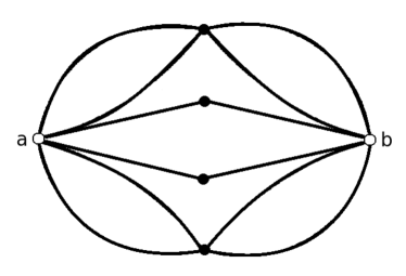
Figure 16: MK lattice with fractal dimension $d=3.58$, the same as WB lattice in Fig. 3.

The BEG model with generic magnetic exchange interaction is defined by the Hamiltonian (we use reduced variables)

$$-{\cal{H}}(s)=\sum_{<ij>}J_{ij}s_{i}s_{j}+K\sum_{<ij>}s^{2}_{i}s^{2}_{j}-\Delta\sum_{i}s^{2}_{i}\,,$$ (35)

where $s_{i}=\pm 1,\,0$ and $J_{ij}$ can be deterministic or quenched disordered and distributed according to some probability distribution. In the latter case, under PSRG transformation all renormalized interactions become quenched random and it is convenient to start the iteration using the more general form

$$-\mathcal{H}=\sum_{\left\langle ij\right\rangle}J_{ij}s_{i}s_{j}+\sum_{\left\langle ij\right\rangle}K_{ij}s^{2}_{i}s^{2}_{j}-\sum_{\left\langle ij\right\rangle}\Delta_{ij}\left(s^{2}_{i}+s^{2}_{j}\right)-\sum_{\left\langle ij\right\rangle}\Delta_{ij}^{\dagger}\left(s^{2}_{i}-s^{2}_{j}\right)$$

The model is, further, defined, by the multivariable initial probability distribution of the interactions:

$${\cal P}(J_{ij},K_{ij},\Delta_{ij},\Delta^{\dagger}_{ij})\!= \!\!\!\!\frac{\delta(J_{ij}-J_{0})+\delta(J_{ij}+J_{0})}{2}\delta(K_{ij})~{}\delta(\Delta_{ij}-\Delta_{0})~{}\delta(\Delta_{ij}^{\dagger})\,.$$

We notice that if $\Delta_{0}\ll-1$, the values $s_{i}=0$ are suppressed and the model tends to the Ising spin glass model analyzed in previous sections:

$$-{\cal{H}}(\{J_{ij}\};\{s_{i}\})=\sum_{\langle ij\rangle}J_{ij}s_{i}s_{j}$$

with $s_{i}=\pm 1$ and

$$P(J_{ij})=\int dK_{ij}\,d\Delta_{ij}\,d\Delta^{\dagger}_{ij}\,{\cal P}(J_{ij},K_{ij},\Delta_{ij},\Delta^{\dagger}_{ij})\,.$$

Decimating the inner sites at a given hierarchical cell with fixed outer sites $s_{a}$ and $s_{b}$, and using the up-down symmetry of the Hamiltonian, the relations for the renormalized interactions imposed by the conservation of the partition function, cf. Eq. (3), can be written similarly to Eqs. (3)-(4) as

$$J_{R} = \frac{1}{2}\log\biggl{(}\frac{x_{++}}{x_{+-}}\biggl{)},\,$$

$$K_{R} = \frac{1}{2}\log\biggl{(}\frac{x_{++}~{}x_{+-}~{}x_{00}^{2}}{x_{0+}^{2}~{}x_{+0}^{2}}\biggl{)},\,$$

$$\Delta_{R} = \frac{1}{2}\log\biggl{(}\frac{x_{00}^{2}}{x_{+0}~{}x_{0+}}\biggl{)}\,,$$ (37)

$$\Delta^{\dagger}_{R} = \frac{1}{2}\log\biggl{(}\frac{x_{+0}}{x_{0+}}\biggl{)}\,,$$

where $x_{s_{a}s_{b}}$ are the edge Boltzmann factors, cf. Eq. (3). In the $T=0$ limit these relations become

$$2J_{R} = \max\bigl{[}-\mathcal{H}(1,1,s)\bigr{]}-\max\bigl{[}-\mathcal{H}(1,-1,s)\bigr{]}$$

$$2K_{R} = \max\bigl{[}-\mathcal{H}(1,1,s))\bigr{]}+\max\bigl{[}-\mathcal{H}(1,-1,s)\bigr{]}$$ (38)

$$-2\bigr{\{}\max\bigl{[}-\mathcal{H}(1,0,s)\bigr{]}-\max\bigl{[}-\mathcal{H}(0,1,s)\bigr{]}\bigr{\}}$$

$$+2\max\bigl{[}-\mathcal{H}(0,0,s)\bigr{]}$$

$$2\Delta_{R} = 2\max\bigl{[}-\mathcal{H}(0,0,s)\bigr{]}$$

$$-\max\bigl{[}-\mathcal{H}(1,0,s)\bigr{]}-\max\bigl{[}-\mathcal{H}(0,1,s)\bigr{]}$$

$$2\Delta^{\dagger}_{R} = \max\bigl{[}-\mathcal{H}(1,0,s)\bigr{]}-\max\bigl{[}-\mathcal{H}(0,1,s)\bigr{]}$$

Figure 17: Phase diagram for the BEG model on the MK$(d=3)$ lattice in Fig. 12, WB lattice in Fig. 3, FC lattice in Fig. 11 and simulations Paoluzzi10 . The line for the MKs and WB are obtained with $M=10^{6}$, whilst for the FC we use $M=5\cdot 10^{4}$. Inset: detail of the reentrance region for WB and 3D cubic lattices, compared to the MK HL line (no reentrance).

The phase diagrams relative to the different hierarchical lattices are shown in Fig. 17. They are obtained representing the probability distributions by a pool of $M=10^{5}$ interaction quadruples $(J,K,\Delta,\Delta^{\dagger})$ and the RG evolution of each distribution is analyzed over $N_{S}=10$ different samples, i.e., starting with ten different initial realizations of the quenched couplings. As worked out in Sec. 2, paramagnetic, ferromagnetic and spin glass phases are determined by the analysis of the PSRG flux of $J=\langle J_{ij}\rangle$ and $\sigma^{2}_{J}=\langle J_{ij}^{2}\rangle-\langle J_{ij}\rangle^{2}$.

In all cases we obtain a second order transition between paramagnetic and spin glass phases, with all points on the transition line attracted by a unique fixed distribution at $\Delta\rightarrow-\infty$ (see Fig. 18), thus belonging to the same universality class of the SG-PM transition in the Ising spin glass investigated in the previous section.

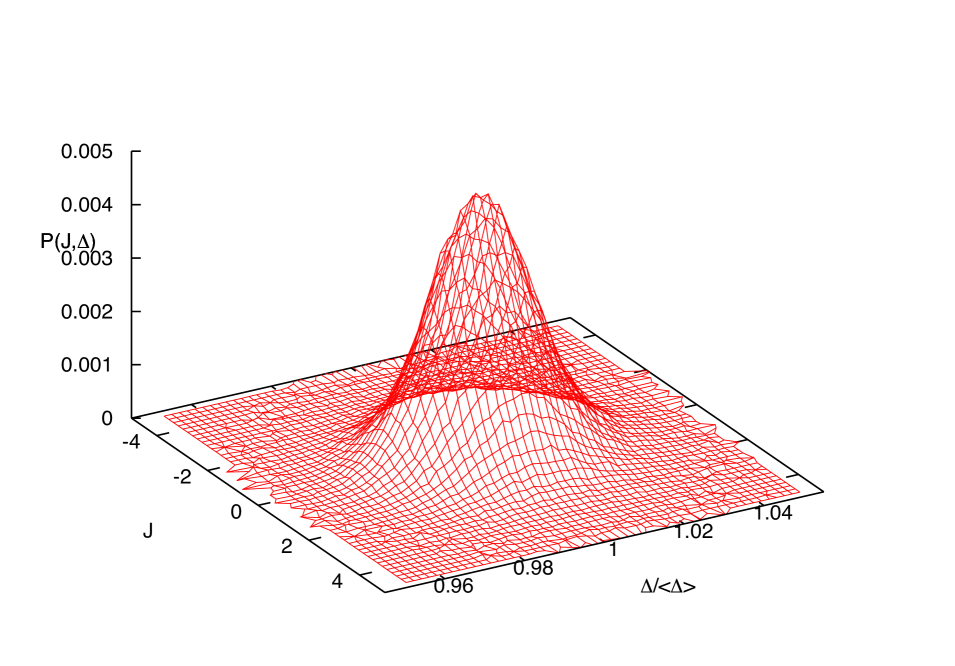
Figure 18: (Projection of unstable fixed distribution ${\cal P}(J,K,\Delta,\Delta^{\dagger})$ for BEG model at the transition SG-para on the WB lattice in Fig. 3. In the distribution $\Delta$ is runaway to minus infinity exponentially, while other interactions remain finite and the distribution retains this shape. The shape of relative distribution on the MK and FC lattices is very similar.

4.1 Lack of first order phase transition

Studying hierarchical lattices also much more complex than MK, the first order transition typical of the BEG model on Bravais lattice is not found, so we have a strong indication that this is an intrinsic limit of hierarchical lattices, and not only of the MK kind of cells.

We have no clear evidence on why the first order transition is missing on the hierarchical lattices lattices we have considered so far. Based on physical arguments we may propose the following hypothesis. Second order transition are associated with an instability, the high temperature phase becomes unstable and a new stable phase appears. This instability can manifest itself locally, and hence hierarchical lattices can show a second order transition. First order transitions, on the contrary, are not triggered by an instability. The high temperature phase remains stable, but a thermodynamically more favorable phase takes over. Such a situation requires some sort of long range structure of the lattice, that is missing in the present hierarchical lattices, and this may explain why we do not see first order transitions. If our conjecture is correct we may wonder if the first order transition could still appear in hierarchical lattices with folded cells for $b$ finite but large enough. However, from our present knowledge this value of $b$ might be so large to make the HL approach ineffective. The analysis of the arising of a possible fist order critical behavior in $b$ is left for future work.

4.2 Inverse freezing

An apart feature of the BEG model arises, instead, adopting WB cells: the inverse transition between spin glass and paramagnet. it occurs in the WB $d\approx 3.58$ where evidence for the reentrance is clearly obtained using the $T=0$ Eqs. (38). Inverse freezing is predicted in mean-field theoryCrisanti05 and found in 3D numerical simulations.Paoluzzi10 . It is not found in MK lattices, instead, neither in fractal dimension $3$ (cf. Fig. 12) nor in $d\approx 3.58$ (cf. Fig. 16) nor in the FC lattice.

5 Conclusions

We have provided a critical review of the standard methods to develop PSRG on hierachical lattices and applied them to different models. On one side this analysis can be useful to test general results (e.g. Nishimori conjecture, Harris criterion), and on the other side it is far easier and faster than Monte Carlo simulations on Bravais lattice. We, however, stress that these methods display several drawbacks that we critically underlined model by model.

We have investigated the Random Field Ising Model (RFIM), the Random Bond Ising Model (RBIM) and the Blume-Emery-Griffiths (BEG) model defined on several MK and non-MK hierachical lattices, obtaining phase diagrams and critical exponents.

The RFIM has been analyzed on a non-MK (WB in Fig. 3) and we show that the bimodal and Gaussian disordered cases belong to the same universality class.

The RBIM in $d<2.5$ has been analyzed on the folded square HLs family for $b=3$ (Fig. 4) and $b=5$ (Fig. 5), where we find that the Nishimori conjecture fails and the disorder is irrelevant.

The RBIM in $d>2.5$ has been analyzed on the folded cube (Fig. 11) and compared to MK (Fig. 12) and WB (Fig. 3), where we obtain the critical exponents for the SG-PM transition and also show that the Harris criterion turns out to be satisfied.

The BEG model has been analyzed on non-MK HLs, i.e., WB (Fig. 3) and folded cube (Fig. 11), and compared to MK with $d=3$ (Fig. 12) and $d\sim 3.58$ (Fig. 16), and in all the cases the first order transition taking place in the Bravais lattice for large enough chemical potential Crisanti05 ; Paoluzzi10 is absent.

Our results provide a clue to the possibility of obtaining approximations of models on regular lattice by similar models on hierachical lattice. We show that it is possible to obtain a good picture of the actual phase diagram, but far more difficult to yield a proper determination of critical exponents.

By introducing more complex elementary cells, with some non trivial internal structure, one hopes of capturing the local geometrical properties of the bonds. At least part of it. For pure models, although it is not a systematic approximation, a general improvement is obtained using unit cells that locally mimic better the connectivity of the Bravais lattice. In the disordered case, instead, the situation is less definite, and no net improvement is observed: the WB cell (Fig. 3) proves to be the slightly most reliable (generally quantitatively better than the more complex folded cube in Fig. 11), and in particular shows the expected inverse transition for the BEG model, but we cannot give a general explanation for this.

In particular, the fractal dimension seems to play a minor role, as the three dimensional regular lattice is better approximated by the WB with $d\sim 3.58$, compared to $d=3$ MK (Fig. 12) and $d\sim 3.24$ folded cube (Fig. 11), while the $d\sim 3.58$ MK in Fig. 16 is the worst approximation by far.

The scaling factor $b$ has the known role to determine if the antiferromagnetic order can be preserved, as it is possible only when $b$ is odd so that negative interactions in the unit cell involve negative interactions between the external sites (and this leads to a phase diagram symmetric under the inversion of the bonds sign). Our results indicates that this feature does not play a crucial role in the disordered systems (at least until the negative bonds become dominant). The two investigated HLs with an even $b$, the WB and the $d\sim 3.58$ MK, indeed, appear to be, respectively, the best and the worst in approximating the phase diagram of the models on regular lattice. The only case in which the folded cube lattice in Fig. 11 provides a remarkable improvement with respect to the WB lattice is in the estimate of the SG stiffness exponent. A more structured inner local connectivity could, thus, become important at low temperatures.

In conclusion, our results show that the approximation on HL is particularly poor for disordered systems, and strongly suggest that its limitations are intrinsic to the hierarchical nature. The most striking case is the lack of first order transition in BEG. Indeed, using more complex HLs we may have a better treatment of short distances, i.e., short loops, but longer distances appear definitely dominated by the hierarchical backbone.

- (1) G. Parisi. Infinite number of order parameters for spin- glasses. Phys. Rev. Lett., 43:1754-1756, 1979.
- (2) G. Parisi. A sequence of approximated solutiona to the S-K model for spin glasses. J. Phys. A: Math. Gen., 13:L115, 1980.
- (3) M. Mézard, G. Parisi, and M. Virasoro. Spin Glass Theory and Beyond. World Scientific (Singapore), 1987.
- (4) D.J. Amit. Modeling Brain Functions: The World of Attractor Neural Networks. Cambridge University Press (Cambridge, U.K.), 1992.
- (5) M. Mézard and A. Montanari. Information, physics, and computation. Oxford University Press (Oxford, U.K.), 2009.
- (6) J.H. Chen and T.C. Lubensky. Mean field and -expansion study of spin glasses. Phys. Rev. B, 16:2106, 1977.
- (7) C. De Dominicis, I. Kondor, and T. Temesvari. Beyond the Sherrington–Kirkpatrick Model. In Directions in Condensed Matter Physics, volume 12, page 119. World Scientific, 1998.
- (8) C. De Dominicis and I. Giardina. Random Fields and Spin Glasses. Cambridge University Press (Cambridge, U.K.), 2006.
- (9) A.J. Bray and M.A. Moore. Disappearance of the de Almeida-Thouless line in six dimensions. Phys. Rev. B, 83:224408, 2011.
- (10) G. Parisi and T. Temesvari. Replica symmetry breaking in and around six dimensions. Nucl. Phys. B [FS], 858:293–316, 2012.
- (11) D.L. Stein and C.M. Newman. Spin Glasses and Complexity. Princeton University Press, 2012.
- (12) D.J. Amit and V. Martin-Mayor. Field Theory; The Renormalization Group and Critical Phenomena. World Scientific, 2005.
- (13) M. Le Bellac. Quantum and Statistical Field Theory. Oxford Science Publications, 1992.
- (14) L.P. Kadanoff. Notes on Migdal’s recursion formulas. Ann. of Phys., 100(1):359–394, 1976.
- (15) S.K. Ma. Modern Theory of Critical Phenomena. Benjamin-Cummings, Reading, 1976.
- (16) J.M.J. Leeuwen Th. Niemeijer. Wilson Theory for Spin Systems on Triangular Lattice. Phys. Rev. Lett., 31(23):1411, 1973.
- (17) A.N. Berker and M. Wortis. Blume-Emery-Griffiths-Potts model in two dimensions: Phase diagram and critical proprieties from a position-space renormalization group. Phys. Rev. B, 14(11):4946, 1976.
- (18) K.H. Fisher W.Kinzel. Existence of a phase transition in spin glasses? J. Phys. C, 11:2115, 1978.
- (19) T. Tatsumi. Renormalization-Group Approach to Spin Glass Transition of a Random Bond Ising Model in Two- and Three-Dimensions. Prog. Theor. Phys., 59:405, 1978.
- (20) S. Franz, G. Parisi, and M.A. Virasoro. Interfaces and louver critical dimension in a spin glass model. J. Phys. I (France), 4:1657, 1994.
- (21) S. Franz and F.L. Toninelli. A field-theoretical approach to the spin glass transition: models with long but finite interaction range. J. Stat. Mech., page P01008, 2005.
- (22) S. Boettcher. Stiffness of the Edwards-Anderson Model in all Dimensions. Phys. Rev. Lett., 95:197205, 2005.
- (23) A.N. Berker and S. Ostlund. Renormalisation-group calculations of finite systems: order parameter and specific heat for epitaxial ordering. J. Phys. C, 12(22):4961, 1979.
- (24) R.B. Griffiths and M. Kaufman. Spin systems on hierarchical lattices. Introduction and thermodynamic limit. Phys. Rev. B, 26:5022–5032, 1982.
- (25) S.R. McKay, A.N. Berker, and S. Kirkpatrick. Spin-Glass Behavior in Frustrated Ising Models with Chaotic Renormalization-Group Trajectories. Phys. Rev. Lett., 48:767–770, 1982.
- (26) M. Ohzeki, H. Nishimori, and A.N. Berker. Multicritical points for spin-glass models on hierarchical lattices. Phys. Rev. E, 77:061116, 2008.
- (27) O.R. Salmon, B.T. Agostini, and F.D. Nobre. Ising spin glasses on Wheatstone–Bridge hierarchical lattices. Phys. Lett. A, 374(15–16):1631–1635, 2010.
- (28) M.A. Moore, H. Bokil, and B. Drossel. Evidence for the Droplet Picture of Spin Glasses. Phys. Rev. Lett., 81:4252, 1998.
- (29) F. Ricci-Tersenghi and F. Ritort. Absence of ageing in the remanent magnetization in Migdal-Kadanoff spin glasses. J. Phys. A: Math. Gen., 33:3727, 2000.
- (30) F.D. Nobre. Phase diagram of the two-dimensional J Ising spin glass. Phys. Rev. E, 64:046108, 2001.
- (31) H. Nishimori and M. Ohzeki. Multicritical point of spin glasses. Phys. A: Stat. Mech. and its Appl., 389:2907–2910, 2010.
- (32) D. Andelman and A.N. Berker. q-state Potts models in dimensions: Migdal-Kadanoff approximation. J. Phys. A: Math. Gen., 14(4):L91, 1981.
- (33) V.O. Ozcelik and A.N. Berker. Blume-Emery-Griffiths spin glass and inverted tricritical points. Phys. Rev. E, 78:031104, 2008.
- (34) L.R. da Silva, C. Tsallis, and G. Schwachheim. Anisotropic cubic lattice Potts ferromagnet: renormalisation group treatment. J. Phys. A: Math. and Gen., 17:3209, 1984.
- (35) C. Tsallis and A.C.N. de Magalhães. Pure and random Potts-like models: real-space renormalization-group approach. Phys. Rep., 268(5–6):305–430, 1996.
- (36) A. Crisanti and L. Leuzzi. Stable solution of the simplest spin model for inverse freezing. Phys, Rev. Lett., 95:087201, 2005.
- (37) M. Paoluzzi, L. Leuzzi, and A. Crisanti. Thermodynamic First Order Transition and Inverse Freezing in a 3D Spin Glass. Phys. Rev. Lett., 104:120602, 2010.
- (38) A. Crisanti, L. Leuzzi, and T. Rizzo. Complexity in mean-field spin glass models: The Ising p-spin. Phys. Rev. B, 71:094202, 2005.
- (39) L. Leuzzi, M. Paoluzzi, and A. Crisanti. Random Blume-Capel model on a cubic lattice: First-order inverse freezing in a three-dimensional spin-glass system. Phys. Rev. B, 83:014107, 2011.
- (40) M. Paoluzzi, L. Leuzzi, and A. Crisanti. The overlap parameter across an inverse first-order phase transition in a 3D spin-glass. Philos. Mag., 91:1966–1976, 2011.
- (41) A.A. Migdal. Phase transitions in gauge and spin-lattice systems. Zh. Eksp. Teor. Fiz., 69:1457, 1975.
- (42) J. Cardy. Scaling and Renormalization in Statistical Physics. Cambridge Lecture Notes in Physics. Cambridge University Press, 1996.
- (43) A.B. Harris and T.C. Lubemsky. Renormalization-Group Approach to the Critical Behavior of Random-Spin Models. Phys. Rev. Lett., 33:1540, 1974.
- (44) D. Andelman and A.N. Berker. Scale-invariant quenched disorder and its stability criterion at random critical points. Phys. Rev. B, 29:2630–2635, 1984.
- (45) A. Falicov and A.N. Berker. Tricritical and Critical End-Point Phenomena under Random Bonds. Phys. Rev. Lett., 76:4380–4383, 1996.
- (46) B.W. Southern and A.P. Young. Real space rescaling study of spin glass behaviour in three dimensions. J. of Phys. C, 10:2179, 1977.
- (47) O.R. Salmon and F.D. Nobre. Spin-glass attractor on tridimensional hierarchical lattices in the presence of an external magnetic field. Phys. Rev. E, 79:051122, 2009.
- (48) A.N. Berker. Comment on “Spin-glass attractor on tridimensional hierarchical lattices in the presence of an external magnetic field”. Phys. Rev. E, 81:043101, 2010.
- (49) A.J. Bray and M.A. Moore. Scaling theory of the random-field Ising model. J. of Phys. C: Solid State Physics, 18(28):L927, 1985.
- (50) M.S. Cao and J. Machta. Migdal-Kadanoff study of the random-field Ising model. Phys. Rev. B, 48:3177–3182, 1993.
- (51) A.N. Berker and S.R. McKay. Modified hyperscaling relation for phase transitions under random fields. Phys. Rev. B, 33:4712–4715, 1986.
- (52) A. Falicov, A.N. Berker, and S.R. McKay. Renormalization-group theory of the random-field Ising model in three dimensions. Phys. Rev. B, 51:8266–8269, 1995.
- (53) A.A. Middleton and D.S. Fisher. Three-dimensional random-field Ising magnet: Interfaces, scaling, and the nature of states. Phys. Rev. B, 65:134411, 2002.
- (54) A.K. Hartmann. Critical exponents of four-dimensional random-field Ising systems. Phys. Rev. B, 65:174427, 2002.
- (55) M. Ohzeki and H. Nishimori. Analytical evidence for the absence of spin glass transition on self-dual lattices. J. Phys. A: Math. Gen., 42:332001, 2009.
- (56) H. Nishimori. Statistical Physics of Spin Glasses and Information Processing: An Introduction. Oxford University Press (Oxford), 2001.
- (57) H. Nishimori and K. Nemoto. Duality and Multicritical Point of Two-Dimensional Spin Glasses. J. Phys. Soc. Jpn., 71:1198, 2002.
- (58) Franz J. Wegner. Duality in Generalized Ising Models and Phase Transitions without Local Order Parameters. J. of Math. Phys., 12(10):2259–2272, 1971.
- (59) F.Y. Wu and Y. K. Wang. Duality transformation in a many-component spin model. J. of Math. Phys., 17(3):439–440, 1976.
- (60) J.M. Maillard, K. Nemoto, and H. Nishimori. Symmetry, complexity and multicritical point of the two-dimensional spin glass. J. Phys. A, 36:9799, 2003.
- (61) K. Takeda and H. Nishimori. Self-dual random-plaquette gauge model and the quantum toric code. Nuc. Phys. B, 686(3):377–396, 2004.
- (62) H. Nishimori. Internal Energy, Specific Heat and Correlation Function of the Bond-Random Ising Model. Prog. Theor. Phys., 66:1169, 1981.
- (63) M. Hinczewski and A.N. Berker. Multicritical point relations in three dual pairs of hierarchical-lattice Ising spin glasses. Phys. Rev. B, 72:144402, 2005.
- (64) F.D.A. Aarão Reis, S.L.A. de Queiroz, and R.R. dos Santos. Universality, frustration, and conformal invariance in two-dimensional random Ising magnets. Phys. Rev. B, 60:6740–6748, 1999.
- (65) Rajiv R.P. Singh and J. Adler. High-temperature expansion study of the Nishimori multicritical point in two and four dimensions. Phys. Rev. B, 54:364–367, 1996.
- (66) Y. Ozeki and N. Ito. Multicritical dynamics for the +/- J Ising Model. J. of Phys. A, 31:5451, 1998.
- (67) A.B. Harris. Effect of random defects on the critical behaviour of Ising models. J. Phys. C: Sol. St. Phys., 7:1671, 1974.
- (68) E. Domany. Some results for the two-dimensional Ising model with competing interactions. J. of Phys. C, 12:L119, 1979.
- (69) M. Ohzeki, C. K. Thomas, H. G. Katzgraber, H. Bombin, and M. A. Martin-Delgado. Lack of universality in phase boundary slopes for spin glasses on self dual lattices. J. of Stat. Mech., 2011.
- (70) N. Kawashima and H. Rieger. Finite-size scaling analysis of exact ground states for +/-J spin glass models in two dimensions. Europhys. Lett., 39:85, 1997.
- (71) J.T. Chayes, L. Chayes, D.S. Fisher, and T. Spencer. Finite-Size Scaling and Correlation Lengths for Disordered Systems. Phys. Rev. Lett., 57:2999–3002, 1986.
- (72) W. Kinzel and E. Domany. Critical properties of random Potts models. Phys. Rev. B, 23:3421–3434, 1981.
- (73) D. Andelman and A. Aharony. Critical behavior with axially correlated random bonds. Phys. Rev. B, 31:4305–4312, 1985.
- (74) B. Derrida, H. Dickinson, and J. Yeomans. On the Harris criterion for hierarchical lattices. J. of Phys. A, 18(1):L53, 1985.
- (75) S. Mukherji and S.M. Bhattacharjee. Failure of the Harris criterion for directed polymers on hierarchical lattices. Phys. Rev. E, 52:1930–1933, 1995.
- (76) A. Efrat. Harris criterion on hierarchical lattices: Rigorous inequalities and counterexamples in Ising systems. Phys. Rev. E, 63:066112, 2001.
- (77) A.J. Bray and M.A. Moore. Lower critical dimension of Ising spin glasses: a numerical study. J. of Phys. C, 17(18):L463, 1984.
- (78) F.D. Nobre. Real-space renormalization-group approaches for two-dimensional Gaussian Ising spin glass. Phys. Lett. A, 250:163, 1998.
- (79) A.J. Bray and M.A. Moore. Heidelberg Colloquium on Glassy Dynamics. In J.L. van Hemmen, editor, Lecture Notes in Phys., volume 275, pages 121–153. Springer-Verlag, Berlin, 1987.
- (80) A.K. Hartmann, A.J. Bray, A.C. Carter, M.A. Moore, and A.P. Young. Stiffness exponent of two-dimensional Ising spin glasses for nonperiodic boundary conditions using aspect-ratio scaling. Phys. Rev. B, 66:224401, 2002.
- (81) M. Weigel and D. Johnston. Frustration effects in antiferromagnets on planar random graphs. Phys. Rev. B, 76:054408, 2007.
- (82) A. Erbas, A. Tuncer, B. Yücesoy, and A.N. Berker. Phase diagrams and crossover in spatially anisotropic Ising, magnetic, and percolation systems: Exact renormalization-group solutions of hierarchical models. Phys. Rev. E, 72:026129, 2005.
- (83) A.L. Talapov and H.W.J. Blöte. The magnetization of the 3D Ising model. J. of Phys. A, 29(17):5727, 1996.
- (84) B. Nienhuis and M. Nauenberg. First-Order Phase Transitions in Renormalization-Group Theory. Phys. Rev. Lett., 35:477–479, 1975.
- (85) A. Pelissetto and E. Vicari. Critical phenomena and renormalization-group theory. Phys. Rep., 368:549–727, 2002.
- (86) H.G. Katzgraber, M. Körner, and A.P. Young. Universality in three-dimensional Ising spin glasses: A Monte Carlo study. Phys. Rev. B, 73(22):224432, 2006.
- (87) T. Jörg and H.G. Katzgraber. Evidence for Universal Scaling in the Spin-Glass Phase. Phys. Rev. Lett., 101(19):197205, 2008.
- (88) M. Hasenbusch, A. Pelissetto, and E. Vicari. Critical behavior of three-dimensional Ising spin glass models. Phys. Rev. B, 78:214205, 2008.
- (89) M. Blume, V.J. Emery, and R.B. Griffiths. Ising Model for the Transition and Phase Separation in - Mixtures. Phys. Rev. A, 4:1071–1077, 1971.
- (90) M. Blume. Theory of the First-Order Magnetic Phase Change in U. Phys. Rev., 141:517, 1966.
- (91) H.W. Capel. On the possibility of first-order phase transitions in Ising systems of triplet ions with zero-field splitting. Physica, 32:966, 1966.
- (92) D. M. Saul, M. Wortis, and D. Stauffer. Tricritical behavior of the Blume-Capel model. Phys. Rev. B, 9:4964, 1974.
- (93) M. Deserno. Tricriticality and the Blume-Capel model: A Monte Carlo study within the microcanonical ensemble. Phys. Rev. E, 56:5204, 1997.
- (94) K.G. Chakraborty. Effective-field model for a spin-1 Ising system with dipolar and quadrupolar interactions. Phys. Rev. B, 29:1454–1457, 1984.
- (95) O.R. Baran and R.R. Levitskii. Reentrant phase transitions in the Blume-Emery-Griffiths model on a simple cubic lattice: The two-particle cluster approximation. Phys. Rev. B, 65:172407, 2002.
- (96) A. Crisanti and L. Leuzzi. First-Order Phase Transition and Phase Coexistence in a Spin-Glass Model. Phys. Rev. Lett., 89:237204, 2002.
- (97) A. Crisanti and F. Ritort. Intermittency of glassy relaxation and the emergence of a non-equilibirum spontaneous measure in the aging regime. Europhys. Lett., 66:253, 2004.
- (98) I. Puha and H.T. Diep. Random-bond and random-anisotropy effects in the phase diagram of the Blume-Capel model. J. Mag. Mag. Mat., 224:85–92, 2000.