Simultaneous extraction of transversity and Collins functions
from new SIDIS and data
M. Anselmino
Dipartimento di Fisica, Università di Torino,
Via P. Giuria 1, I-10125 Torino, Italy
INFN, Sezione di Torino, Via P. Giuria 1, I-10125 Torino, Italy
M. Boglione
Dipartimento di Fisica, Università di Torino,
Via P. Giuria 1, I-10125 Torino, Italy
INFN, Sezione di Torino, Via P. Giuria 1, I-10125 Torino, Italy
U. D’Alesio
Dipartimento di Fisica, Università di Cagliari,
Cittadella Universitaria, I-09042 Monserrato (CA), Italy
INFN, Sezione di Cagliari,
C.P. 170, I-09042 Monserrato (CA), Italy
S. Melis
Dipartimento di Fisica, Università di Torino,
Via P. Giuria 1, I-10125 Torino, Italy
INFN, Sezione di Torino, Via P. Giuria 1, I-10125 Torino, Italy
F. Murgia
INFN, Sezione di Cagliari,
C.P. 170, I-09042 Monserrato (CA), Italy
A. Prokudin
Jefferson Laboratory, 12000 Jefferson Avenue, Newport News, VA 23606, USA
Abstract
We present a global re-analysis of the most recent experimental
data on azimuthal asymmetries in semi-inclusive deep inelastic
scattering, from the HERMES and COMPASS Collaborations, and
in processes, from the Belle Collaboration.
The transversity and the Collins functions are extracted simultaneously,
in the framework of a revised analysis in which a new
parameterisation of the Collins functions is also tested.
pacs:
13.88.+e, 13.60.-r, 13.66.Bc, 13.85.Ni
††preprint: JLAB-THY-13-1704
I Introduction and formalism
The spin structure of the nucleon, in its partonic collinear configuration,
is fully described, at leading-twist, by three independent Parton Distribution Functions (PDFs): the unpolarised PDF, the helicity distribution and
the transversity distribution. While the unpolarised PDF and the helicity distribution, which have been studied for decades, are by now very
well or reasonably well known, much less information is available on
the latter, which has been studied only recently. The reason is that, due
to its chiral-odd nature, a transversity distribution can only be accessed
in processes where it couples to another chiral-odd quantity.
The chiral-odd partner of the transversity distribution could be a
fragmentation function, like the Collins function Collins (1993)
or the di-hadron fragmentation function Collins et al. (1994); Jaffe et al. (1998); Radici et al. (2002) or another parton distribution, like the
Boer-Mulders Boer and Mulders (1998) or the transversity distribution itself.
A chiral-odd partonic distribution couples to a chiral-odd fragmentation
function in Semi-Inclusive Deep Inelastic Scattering processes (SIDIS,
). The coupling of two chiral-odd partonic
distributions could occur in Drell-Yan processes (D-Y, ) but, so far, no data on polarised D-Y is available.
Information on the convolution of two chiral-odd fragmentation functions
(FFs) can be obtained from processes.
The and quark transversity distributions, together with the Collins
fragmentation functions, have been extracted for the first time in
Refs. Anselmino et al. (2007); Anselmino
et al. (2009a), from a combined analysis
of SIDIS and data. Similar results on the transversity distributions,
coupled to the di-hadron, rather than the Collins, fragmentation function,
have been obtained recently Bacchetta et al. (2012). These independent results
establish with certainty the role played by the transversity distributions in
SIDIS azimuthal asymmetries.
Since the first papers Anselmino et al. (2007); Anselmino
et al. (2009a),
new data have become available: from the COMPASS experiment operating on
a transversely polarised proton
(NH3 target) Adolph et al. (2012); Martin (2013),
from a final analysis of the HERMES Collaboration Airapetian et al. (2010)
and from corrected results of the Belle Collaboration Seidl et al. (2012).
This fresh information motivates a new global analysis for the simultaneous extraction of the transversity distributions and the Collins functions.
This is performed using techniques similar to those implemented in
Refs. Anselmino et al. (2007); Anselmino
et al. (2009a); in addition, a second,
different parameterisation of the Collins function will be tested, in order
to assess the influence of a particular functional form on our results.
Let us briefly recall the strategy followed and the formalism adopted in
extracting the transversity and Collins distribution functions from
independent SIDIS and data.
I.1 SIDIS
We consider, at , the SIDIS process and the single spin asymmetry,
(1)
where is a shorthand notation for
and are the usual SIDIS variables:
(2)
We adopt here the same notations and kinematical variables as defined in
Refs. Anselmino et al. (2007, 2011), to which we refer for
further details, in particular for the definition of the azimuthal angles
which appear above and in the following equations.
By considering the moment of
Bacchetta et al. (2007), we are able to single out the effect
originating from the spin dependent part of the fragmentation function
of a transversely polarised quark, embedded in the Collins function,
Bacchetta et al. (2004), coupled to the TMD
transversity distribution Anselmino et al. (2007):
(3)
where , and
(4)
The usual integrated transversity distribution is given, according to
some common notations, by:
(5)
This analysis, performed at , can be further simplified
adopting a Gaussian and factorized parameterization of the TMDs. In particular
for the unpolarized parton distribution (TMD-PDFs) and fragmentation
(TMD-FFs) functions we use:
(6)
(7)
with and fixed
to the values found in Ref. Anselmino et al. (2005) by analyzing
unpolarized SIDIS azimuthal dependent data:
(8)
The integrated parton distribution and fragmentation functions,
and , are available in the literature; in
particular, we use the GRV98LO PDF set Gluck et al. (1998) and the
DSS fragmentation function set de Florian et al. (2007).
For the transversity distribution, , and
the Collins FF, , we adopt the
following parameterizations Anselmino et al. (2007):
(9)
(10)
with
(11)
(12)
(13)
and , . We assume
. The combination , where
is the helicity distribution, is evolved in
according to Ref. Vogelsang (1998). Notice that with these
choices both the transversity and the Collins function automatically
obey their proper positivity bounds. A different functional form of
will be explored in Section II.2.
Using these parameterizations we obtain the following expression for
:
(14)
with
(15)
When data or phenomenological information at different values are
considered, we take into account, at leading order (LO), the QCD evolution
of the integrated transversity distribution. For the Collins FF,
, as its scale dependence is unknown, we
tentatively assume the same evolution as for the unpolarized FF,
.
I.2 processes
Remarkably, independent information on the Collins functions can be
obtained in unpolarized processes, by looking at the azimuthal correlations of hadrons produced in opposite jets Boer et al. (1997).
This has been performed by the Belle Collaboration, which have measured
azimuthal hadron-hadron correlations for inclusive charged pion production,
Seidl et al. (2006, 2008, 2012).
This correlation can be interpreted as a direct measure of the Collins
effect, involving the convolution of two Collins functions.
Two methods have been adopted in the experimental analysis of the Belle
data. These can be schematically described as (for further details and
definitions see Refs. Boer et al. (1997); Anselmino et al. (2007); Seidl et al. (2008)):
the “ method” in the
Collins-Soper frame where the jet thrust axis is used as the direction and the scattering defines the
plane; and are the azimuthal angles
of the two hadrons around the thrust axis;
the “ method”, using the Gottfried-Jackson
frame where one of the produced hadrons () identifies the
direction and the plane is determined by the
lepton and the directions. There will then be another relevant
plane, determined by and the direction of the other
observed hadron , at an angle with respect to the
plane.
In both cases one integrates over the magnitude of the intrinsic
transverse momenta of the hadrons with respect to the fragmenting
quarks. For the method the
cross section for the process reads:
(16)
where is the angle between the lepton direction and the
thrust axis and
(17)
Integrating over the covered values of and normalizing to the
corresponding azimuthal averaged unpolarized cross section one has:
(18)
For the method, with the Gaussian ansatz
(10), the analogue of Eq. (18) reads
(19)
where is now the angle between the lepton and the
hadron directions.
can be found in the experimental data (see Tables IV and V of
Ref. Seidl et al. (2008)).
To eliminate false asymmetries, the Belle Collaboration consider the
ratio of unlike-sign ( + )
to like-sign ( + ) or charged
( + + )
pion pair production, denoted respectively with indices , and .
For example, in the case of unlike- to like-pair production, one has
(21)
(22)
and
(23)
(24)
and similarly for and .
Explicitely, one has:
(25)
(26)
(27)
(28)
(29)
For fitting purposes, it is convenient to introduce favoured and
disfavoured fragmentation functions, assuming in Eq. (10):
(30)
(31)
with the corresponding relations for the integrated Collins functions,
Eq. (17), and with as
given in Eq. (12) with .
We can now perform a best fit of the data from HERMES and COMPASS on
and of the data, from the Belle
Collaboration, on and . Their expressions,
Eqs. (14) and (25)–(31), contain the transversity and the Collins functions, parameterised as in
Eqs. (9)–(13). They depend on the free
parameters and .
Following Ref. Anselmino et al. (2007) we assume the exponents
and the mass scale to be flavour independent and consider the transversity
distributions only for and quarks (with the two free parameters
and ). The favoured and disfavoured Collins functions
are fixed, in addition to the flavour independent exponents and
, by and . This makes a total
of 9 parameters, to be fixed with a best fit procedure.
Notice that while in the present analysis we can safely neglect
any flavour dependence of the parameter (which is anyway hardly
constrained by the SIDIS data), this issue could play a significant role
in other studies, like those discussed in Ref. Anselmino
et al. (2012a).
II Best fits, results and parameterisations
II.1 Standard parameterisation
We start by repeating the same fitting procedure as in
Refs. Anselmino et al. (2007); Anselmino
et al. (2009a), using the same
“standard” parameterisation, Eqs. (6)–(13),
with the difference that now we include all the most recent SIDIS data
from COMPASS Martin (2013) and HERMES Airapetian et al. (2010) Collaborations, and the corrected Belle data Seidl et al. (2012) on
and . Notice, in particular, that the
data are included in our fits for the first time here.
In fact, a previous inconsistency between and
data, present in the first Belle results Seidl et al. (2006),
has been removed in Ref. Seidl et al. (2012).
The results we obtain are remarkably good, with a total
of , as reported in the first line of Table 1,
and the values of the resulting parameters, given in Table 2,
are consistent with those found in our previous extractions. Our best
fits are shown in Fig. 1 (upper plots), for
the Belle data, in Fig. 2 for the SIDIS
COMPASS data and in Fig. 3 for the HERMES results.
Table 1: Summary of the values obtained in our fits.
The columns, from left to right give the per degree of freedom,
the total , and the separate contributions to the total
of the data from SIDIS, , , and
. “NO FIT” means that the for that set of data
does not refer to a best fit, but to the computation of the corresponding
quantity using the best fit parameters fixed by the other data.
The four lines show the results for the two choices of parameterisation of
the dependence of the Collins functions (standard and polynomial)
and for the two independent sets of data fitted (SIDIS, ,
and SIDIS, , ).
FIT DATA
SIDIS
178 points
146 points
16 points
16 points
16 points
16 points
Standard
Parameterization
NO FIT
NO FIT
Standard
Parameterization
NO FIT
NO FIT
Polynomial
Parameterization
NO FIT
NO FIT
Polynomial
Parameterization
NO FIT
NO FIT
Table 2:
Best values of the 9 free parameters fixing the and quark
transversity distribution functions and the favoured and
disfavoured Collins fragmentation functions, as obtained by fitting
simultaneously SIDIS data on the Collins asymmetry and Belle data on
and . The transversity distributions are parameterised according to Eqs. (9), (11) and the Collins
fragmentation functions according to the standard parameterisation,
Eqs. (10), (12) and (13). We obtain a
total . The statistical errors quoted for each
parameter correspond to the shaded uncertainty areas in
Figs. 1–3,
as explained in the text and in the Appendix of Ref. Anselmino
et al. (2009b).
=
=
=
=
=
=
=
=
GeV2
We have not inserted the Belle data in our global analysis
as they are strongly correlated with the results, being a
different analysis of the same experimental events. However,
using the extracted parameters we can compute the and
azimuthal asymmetries, in good qualitative agreement with
the Belle measurements, although the corresponding values are
rather large, as shown in Table 1. These results are
presented in Fig. 1 (lower plots).
Figure 1:
The experimental data on , (upper plots)
and and (lower plots), as measured
by the Belle Collaboration Seidl et al. (2012) in unpolarized
processes, are compared to
the curves obtained from our global fit. The solid lines correspond
to the parameters given in Table 2, obtained by fitting the
SIDIS and the asymmetries with the standard parameterisation;
the shaded areas correspond to the statistical uncertainty on the
parameters, as explained in the text and in Ref. Anselmino
et al. (2009b).
Notice that the and data are not included in
the fit and our curves, with the corresponding uncertainties, are
simply computed using the parameters of Table 2.
The shaded uncertainty bands are computed according to the procedure
explained in the Appendix of Ref. Anselmino
et al. (2009b). We have
allowed the set of best fit parameters to vary in such a way that
the corresponding new curves have a total which differs from
the best fit by less than a certain amount .
All these (1500) new curves lie inside the shaded area. The chosen value
of is such that the probability to find the “true”
result inside the shaded band is 95.45%.
We have also performed a global fit based on the SIDIS and Belle
data, and then computed the values. We do not show the best fit
plots, which are not very informative, but the quality of the results
can be judged from the second line of Table 1, which shows that
although this time and are actually
fitted, their corresponding values remain large. This has
induced us to explore a different functional shape for the
parameterisation of , Eq. (12),
which will be discussed in the next Subsection.
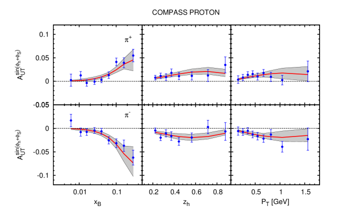
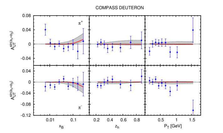
Figure 2:
The experimental data on the SIDIS azimuthal moment as measured by the COMPASS Collaboration Martin (2013)
on proton (upper plots) and deuteron (lower plots) targets, are compared
to the curves obtained from our global fit.
The solid lines correspond to the parameters given in Table 2, obtained by fitting the SIDIS and the asymmetries with standard
parameterisation; the shaded areas correspond to the statistical
uncertainty on the parameters, as explained in the text and in
Ref. Anselmino
et al. (2009b).
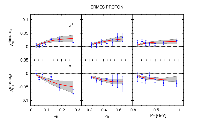
Figure 3:
The experimental data on the SIDIS azimuthal moment as measured by the HERMES Collaboration Airapetian et al. (2010),
are compared to the curves obtained from our global fit. The solid lines
correspond to the parameters given in Table 2, obtained by
fitting the SIDIS and the asymmetries with standard
parameterisation; the shaded areas correspond to the statistical
uncertainty on the parameters, as explained in the text and in
Ref. Anselmino
et al. (2009b).
The difference between and is a delicate issue, that
deserves some further comments. On the experimental side, the hadronic-plane
method used for the extraction of implies a simple analysis
of the raw data, as it requires the sole reconstruction of the
tracks of the two detected hadrons; therefore it leads to very clean
data points, with remarkably small error bars.
On the contrary, the thrust-axis method is much more involved as it
requires the reconstruction of the original direction of the and
which fragment into the observed hadrons; this makes the
measurement of the asymmetry experimentally more challenging,
and leads to data points whith larger uncertainties.
On the theoretical side, the situation is just the opposite: as the
thrust-axis method assumes a perfect knowledge of the and
directions, the asymmetry can be reconstructed by a straightforward
integration over the two intrinsic transverse momenta
and , transforming the convolution of two Collins functions
into the much simpler product of two Collins
moments Anselmino et al. (2007), Eqs. (17) and (18).
Instead, the phenomenological partonic expression of requires
more assumptions and approximations and is, on the theoretical side,
less clean.
One should also add that most of the large values found when
computing from the parameters of a best fit involving SIDIS
and data (or vice-versa) originate from the experimental
points at large values of or or both (see, for example
the last points on the left lower panel in
Fig. 1). Large values of bring us
near the exclusive process limit, where our factorized inclusive
approach cannot hold anymore.
II.2 Polynomial parameterisation
In an attempt to fit equally well and
(keeping in mind, however, the comments at the end of the previous
Subsection) we have explored a possible new parameterisation of the
dependence of the Collins function. We notice that data on
seem to favour an increase at large values, rather
then a decrease, which is implicitly forced by a behaviour of the kind
given in Eqs. (10) and (12) (at least
with positive values).
In addition, an increasing trend of and seems
to be confirmed by very interesting preliminary results of the BABAR
Collaboration, which have performed an independent new analysis of
data Garzia (2012), analogous to
that of Belle.
This suggests that a different parameterisation of the dependence
of favoured and disfavoured Collins functions could turn out to be more
convenient. Then, we try an alternative polynomial parameterisation which
allows more flexibility on the behaviour of at
large :
(32)
with the subfix , and ; and
are flavour independent so that the total number of parameters for
the Collins functions (in addition to ) remains 4. Such a choice
fixes the term to be equal to at and
not larger than at . Notice that we do not automatically impose,
as in Eq. (12), the condition ;
however, we have explicitly checked that the best fit results and all
the sets of parameters corresponding to curves inside the shaded
uncertainty bands satisfy that condition.
We have repeated the same fitting procedure as performed with the standard
parameterisation. When fitting the combined SIDIS, and
Belle data, the resulting best fits (not shown) hardly
exhibit any difference with respect to those obtained with the standard
parameterisation (Fig. 1). This can be
seen also from the ’s in Table 1, where the third line
is very similar to the first one. As a further confirmation, the
corresponding best fit plots for , in
case of the standard and polynomial parameterisations, plotted in
Fig. 4 (left panel) practically coincide up to values of
very close to 1.
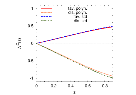
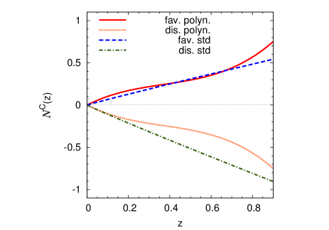
Figure 4:
Plots of the functions and
for the favoured and disfavoured Collins
functions as obtained by using the standard, Eq. (12), and
polynomial, Eq. (32), parameterisations. On the left panel
we show the results obtained by
fitting the SIDIS data together with the Belle asymmetries
(both with standard and polynomial parameterisation), while on the right
panel we show the corresponding results obtained by fitting the SIDIS
data together with the Belle asymmetries.
The situation is different when best fitting the SIDIS data together
with and ; in such a case the polynomial
parameterisation allows a much better best fit, as shown in
Fig. 5, upper plots. A reasonable agreement
can also be achieved between the data and the computed values of
and , as shown by the values
in Table 1 and by the lower plots in Fig. 5.
In this case the polynomial form of
differs from the standard one, as shown in the right plots in
Fig. 4.
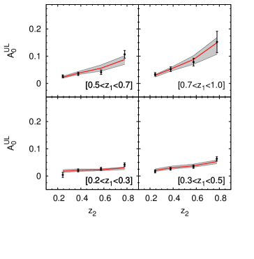
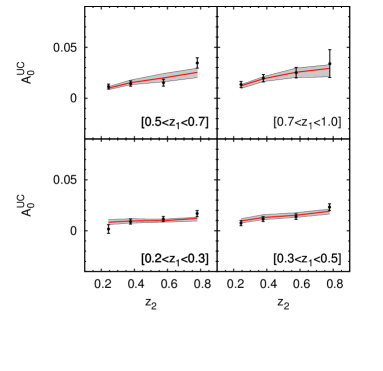
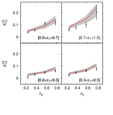
Figure 5:
The experimental data on , (upper plots) and
and (lower plots), as measured by the
Belle Collaboration Seidl et al. (2012) in unpolarized
processes, are compared to the curves
obtained from our global fit. The solid lines correspond to the
parameters given in Table 3, obtained by fitting the
SIDIS and the asymmetries with polynomial parameterisation;
the shaded areas correspond to the statistical uncertainty on the
parameters, as explained in the text and in Ref. Anselmino
et al. (2009b).
Notice that the and data are not included in
the fit and our curves, with the corresponding uncertainties, are
simply computed using the parameters of Table 3.
Notice, again, that the large values of the computed
is almost completely due to the last bins, which correspond to the quasi exclusive region. Also, the larger values corresponding to SIDIS
data are mainly due to a slightly worse description of HERMES azimuthal moments. The values of the parameters obtained using the polynomial shape
of , Eq. (32), are given in
Table 3.
Table 3:
Best values of the 9 free parameters fixing the and quark
transversity distribution functions and the favoured and
disfavoured Collins fragmentation functions, as obtained by fitting
simultaneously SIDIS data on the Collins asymmetry and Belle data on
and . The transversity distributions
are parameterised according to Eqs. (9), (11)
and the Collins fragmentation functions according to the polynomial
parameterisation, Eqs. (10), (32) and
(13). We obtain a total .
The statistical errors quoted for each parameter correspond to the shaded
uncertainty areas in Fig. 5, as explained in the
text and in the Appendix of Ref. Anselmino
et al. (2009b).
=
=
=
=
=
=
=
=
GeV2
II.3 The extracted transversity and Collins functions; predictions and final comments
Our newly extracted transversity and Collins functions are shown in
Figs. 6 and 7; to be
precise, in the left panels we show ,
for and quarks, while in the right panels we plot:
(33)
for and . The Collins results for quark are
not shown explicitly, but could be obtained from Tables 2
and 3.
Fig. 6 shows the results which best fit the
COMPASS and HERMES SIDIS data on ,
together with the Belle results on and ,
using the standard parameterisation. The red solid lines correspond
to the parameters given in Table 2. The shaded bands show
the uncertainty region, which is the region spanned by the 1500
different sets of parameters fixed according to the procedure explained
above and in the Appendix of Ref. Anselmino
et al. (2009b). The blue
dashed lines show, for comparison, our previous
results Anselmino
et al. (2009a): the difference between the solid red
and dashed blue lines is only due to the updated SIDIS and
data used here, with the addition of , while keeping the
same parameterisation. The present and previous results agree within the
uncertainty band: one could at most notice a slight decrease of the
new quark transversity distribution at large values.
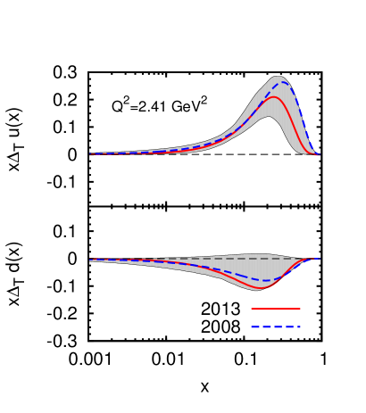
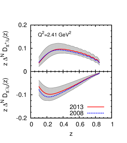
Figure 6:
In the left panel we plot (solid red lines) the transversity
distribution functions for ,
with their uncertainty bands (shaded areas), obtained from our best fit
of SIDIS data on and data on
, adopting the standard parameterisation (Table 2).
Similarly, in the right panel we plot the corresponding first moment of
the favoured and disfavoured Collins functions, Eq. (33). All
results are given at GeV2.
The dashed blue lines show the same quantities as obtained in
Ref. Anselmino
et al. (2009a) using the data then available on
and .
Fig. 7 shows the results which best fit the
COMPASS and HERMES SIDIS data on ,
together with the Belle results on and ,
using the polynomial parameterisation. The red solid lines correspond
to the parameters given in Table 3. This is not a simple
updating of our previous 2008 fit Anselmino
et al. (2009a), as we use
different sets of data (SIDIS and rather than SIDIS
and ) with a different polynomial parameterisation. In this case
the comparison with the 2008 results is less significant. If comparing the
results of Fig. 6 and 7,
one notices a sizeable difference in the favoured ) Collins
function, and less evident differences in the transversity distributions.
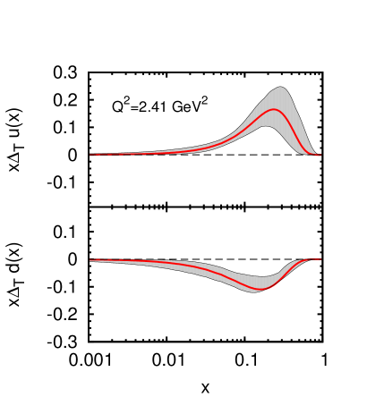
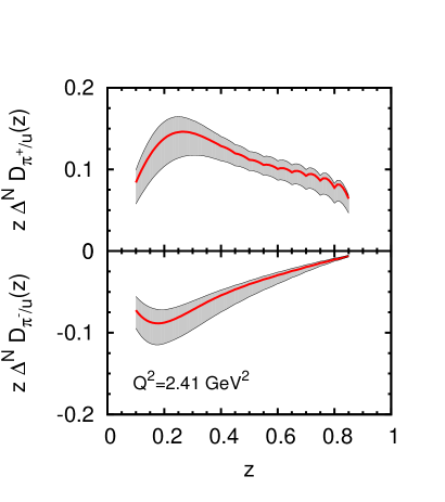
Figure 7:
In the left panel we plot (solid red lines) the transversity
distribution functions for ,
with their uncertainty bands (shaded areas), obtained from our best fit
of SIDIS data on and data on
, adopting the polynomial parameterisation (Table 3).
Similarly, in the right panel we plot the corresponding first moment of
the favoured and disfavoured Collins functions, Eq. (33). All
results are given at GeV2.
In Fig. 8 we show, for comparison with similar results presented in Ref. Anselmino
et al. (2009a), the tensor charge, corresponding
to our best fit transversity distributions, as given in Tables 2
and 3. Our extracted values are shown at GeV2
and compared with several model computations. One should keep in mind that
our estimates are based on the assumption of a negligible contribution from
sea quarks and on a set of data which still cover a limited range of
values.
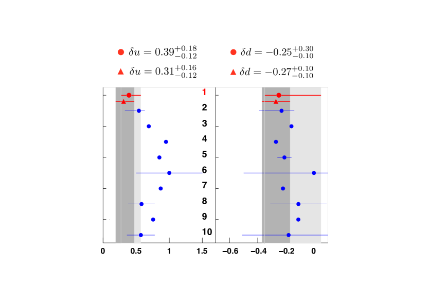
Figure 8:
The tensor charge
for (left) and (right) quarks, computed using the transversity
distributions obtained from our best fits, Table 2 (top solid red
circles) and Table 3 (solid red triangles). The gray areas
correspond to the statistical uncertainty bands in our extraction. These
results are compared with those given in Ref. Anselmino
et al. (2009a)
(number 2) and with the results of the model calculations of
Refs. Cloet et al. (2008); Wakamatsu (2007); Gockeler et al. (2005); He and Ji (1995); Pasquini et al. (2007); Gamberg and Goldstein (2001); Hecht et al. (2001); Bacchetta et al. (2012)
(respectively, numbers 10 and 3-9).
All other results are shown at the scale GeV2. The evolution
to the chosen value has been obtained by evolving at LO the collinear part
of the factorized distribution and fragmentation functions. The TMD
evolution, which might affect the and dependence, is not
yet known for the Collins function. Consistently, it has not been taken
into account for the other distribution and fragmentation functions.
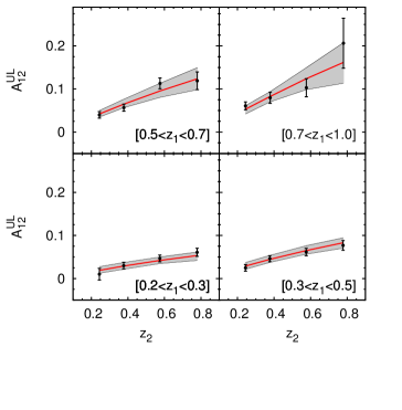
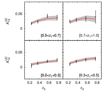
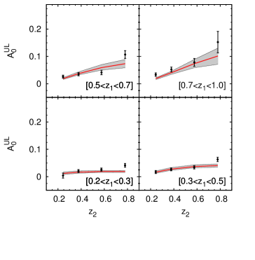
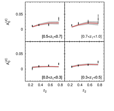
As BABAR data on and should be available soon, we
show in Figs. 9 and 10
our expectations, based on our extracted Collins functions.
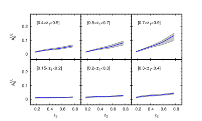
Fig. 9 shows the expected values of
, , and , as
a function of for different bins of , using the parameters
of Table 2, obtained by fitting the SIDIS and the
Belle data with the standard parameterisation.
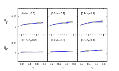
Fig. 10 shows the same quantities using the
parameters of Table 3, obtained by fitting the SIDIS
and the Belle data with the polynomial parameterisation.
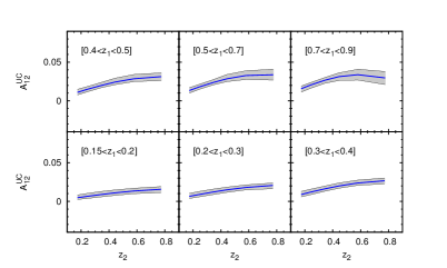
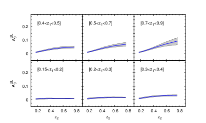
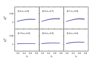
Figure 9:
Estimates, obtained from our global fit, for the azimuthal correlations
, , and in unpolarized
processes at BaBar Garzia (2012).
The solid lines correspond to the parameters given in Table 2,
obtained by fitting the Belle asymmetry; the shaded area
corresponds to the uncertainty on these parameters, as explained in the text.
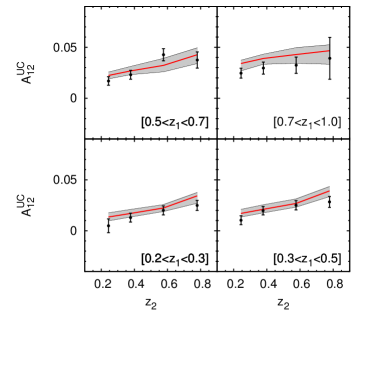
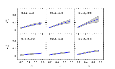
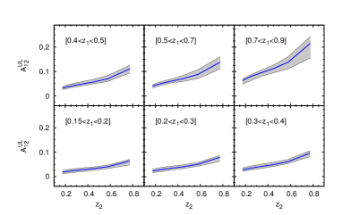
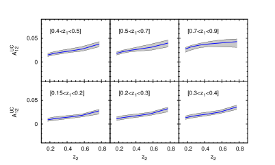
Figure 10:
Estimates, obtained from our global fit, for the azimuthal correlations
, , and in unpolarized
processes at BaBar Garzia (2012).
The solid lines correspond to the parameters given in Table 3, obtained by fitting the Belle asymmetry; the shaded area
corresponds to the uncertainty on these parameters, as explained in the text.
The Belle (and BABAR) results on the azimuthal correlations of
hadrons produced in opposite jets, together with the SIDIS data on the
azimuthal asymmetry , measured by both
the HERMES and COMPASS Collaborations, definitely establish the
importance of the Collins effect in the fragmentation of a transversely polarised quark. In addition, the SIDIS asymmetry can only be observed
if coupled to a non negligible quark transversity distribution.
The first original extraction of the transversity distribution and
the Collins fragmentation functions Anselmino et al. (2007); Anselmino
et al. (2009a), has been confirmed here, with new data and a possible
new functional shape of the Collins functions. The results on the
transversity distribution have also been confirmed independently in
Ref. Bacchetta et al. (2012).
A further improvement in the QCD analysis of the experimental data,
towards a more complete understanding of the Collins and transversity
distributions, and their possible role in other processes, would require
taking into account the TMD-evolution of and
. Great progress has been recently
achieved in the study of the TMD-evolution of the unpolarized and Sivers
transverse momentum dependent distributions Collins (2011); Aybat and Rogers (2011); Aybat et al. (2012a, b); Anselmino
et al. (2012b)
and a similar progress is expected soon for the Collins function and the
transversity TMD distribution Bacchetta and Prokudin (2013).
Acknowledgements.
Authored by a Jefferson Science Associate, LLC under U.S. DOE Contract
No. DE-AC05-06OR23177.
We acknowledge support from the European Community under the FP7
“Capacities - Research Infrastructures” program (HadronPhysics3,
Grant Agreement 283286). We also acknowledge support by MIUR under
Cofinanziamento PRIN 2008.
U.D. is grateful to the Department of Theoretical Physics II of the
Universidad Complutense of Madrid for the kind hospitality extended to him
during the completion of this work.
References
Collins (1993)
J. C. Collins,
Nucl. Phys. B396,
161 (1993).
Collins et al. (1994)
J. C. Collins,
S. F. Heppelmann,
and G. A.
Ladinsky, Nucl. Phys.
B420, 565 (1994).
Jaffe et al. (1998)
R. Jaffe,
X.-m. Jin, and
J. Tang,
Phys. Rev. Lett. 80,
1166 (1998).
Radici et al. (2002)
M. Radici,
R. Jakob, and
A. Bianconi,
Phys. Rev. D65,
074031 (2002).
Boer and Mulders (1998)
D. Boer and
P. Mulders,
Phys. Rev. D57,
5780 (1998).
Anselmino et al. (2007)
M. Anselmino,
M. Boglione,
U. D’Alesio,
A. Kotzinian,
F. Murgia, and
A. Prokudin,
Phys. Rev. D75,
054032 (2007).
Anselmino
et al. (2009a)
M. Anselmino,
M. Boglione,
U. D’Alesio,
A. Kotzinian,
S. Melis,
F. Murgia, and
A. Prokudin,
Nucl. Phys. Proc. Suppl. 191,
98 (2009a).
Bacchetta et al. (2012)
A. Bacchetta,
A. Courtoy, and
M. Radici
(2012), arXiv:1212.3568 [hep-ph].
Adolph et al. (2012)
C. Adolph et al.
(COMPASS Collaboration), Phys.
Lett. B717, 376
(2012).
Martin (2013)
A. Martin
(COMPASS Collaboration) (2013),
arXiv:1303.2076 [hep-ex].
Airapetian et al. (2010)
A. Airapetian
et al. (HERMES Collaboration),
Phys. Lett. B693,
11 (2010).
Seidl et al. (2012)
R. Seidl et al.
(Belle Collaboration), Phys. Rev.
D86, 032011(E)
(2012).
Anselmino et al. (2011)
M. Anselmino,
M. Boglione,
U. D’Alesio,
S. Melis,
F. Murgia,
E. Nocera, and
A. Prokudin,
Phys. Rev. D83,
114019 (2011).
Bacchetta et al. (2007)
A. Bacchetta,
M. Diehl,
K. Goeke,
A. Metz,
P. J. Mulders,
and M. Schlegel,
JHEP 0702, 093
(2007).
Bacchetta et al. (2004)
A. Bacchetta,
U. D’Alesio,
M. Diehl, and
C. A. Miller,
Phys. Rev. D70,
117504 (2004).
Anselmino et al. (2005)
M. Anselmino,
M. Boglione,
U. D’Alesio,
A. Kotzinian,
F. Murgia, and
A. Prokudin,
Phys. Rev. D71,
074006 (2005).
Gluck et al. (1998)
M. Gluck,
E. Reya, and
A. Vogt,
Eur. Phys. J. C5,
461 (1998).
de Florian et al. (2007)
D. de Florian,
R. Sassot, and
M. Stratmann,
Phys. Rev. D75,
114010 (2007).
Vogelsang (1998)
W. Vogelsang,
Phys. Rev. D57,
1886 (1998).
Boer et al. (1997)
D. Boer,
R. Jakob, and
P. J. Mulders,
Nucl. Phys. B504,
345 (1997).
Seidl et al. (2006)
R. Seidl et al.
(Belle Collaboration), Phys. Rev.
Lett. 96, 232002
(2006).
Seidl et al. (2008)
R. Seidl et al.
(Belle Collaboration), Phys. Rev.
D78, 032011
(2008).
Anselmino
et al. (2012a)
M. Anselmino,
M. Boglione,
U. D’Alesio,
E. Leader,
S. Melis,
F. Murgia, and
A. Prokudin,
Phys. Rev. D86,
074032 (2012a).
Anselmino
et al. (2009b)
M. Anselmino,
M. Boglione,
U. D’Alesio,
A. Kotzinian,
S. Melis,
F. Murgia,
A. Prokudin, and
C. Turk,
Eur. Phys. J. A39,
89 (2009b).
Garzia (2012)
I. Garzia
(BABAR Collaboration) (2012),
arXiv:1211.5293 [hep-ex].
Cloet et al. (2008)
I. Cloet,
W. Bentz, and
A. W. Thomas,
Phys. Lett. B659,
214 (2008).
Wakamatsu (2007)
M. Wakamatsu,
Phys. Lett. B653,
398 (2007).
Gockeler et al. (2005)
M. Gockeler et al.
(QCDSF Collaboration, UKQCD Collaboration),
Phys. Lett. B627,
113 (2005).
He and Ji (1995)
H.-x. He and
X.-D. Ji,
Phys. Rev. D52,
2960 (1995).
Pasquini et al. (2007)
B. Pasquini,
M. Pincetti, and
S. Boffi,
Phys. Rev. D76,
034020 (2007).
Gamberg and Goldstein (2001)
L. P. Gamberg and
G. R. Goldstein,
Phys. Rev. Lett. 87,
242001 (2001).
Hecht et al. (2001)
M. Hecht,
C. D. Roberts,
and S. Schmidt,
Phys. Rev. C64,
025204 (2001).
Collins (2011)
J. Collins,
Foundations of perturbative QCD, Cambridge monographs on
particle physics, nuclear physics and cosmology, N. 32, Cambridge University
Press, Cambridge (2011).
Aybat and Rogers (2011)
S. M. Aybat and
T. C. Rogers,
Phys. Rev. D83,
114042 (2011).
Aybat et al. (2012a)
S. M. Aybat,
J. C. Collins,
J.-W. Qiu, and
T. C. Rogers,
Phys. Rev. D85,
034043 (2012a).
Aybat et al. (2012b)
S. M. Aybat,
A. Prokudin, and
T. C. Rogers,
Phys. Rev. Lett. 108,
242003 (2012b).
Anselmino
et al. (2012b)
M. Anselmino,
M. Boglione, and
S. Melis,
Phys. Rev. D86,
014028 (2012b).
Bacchetta and Prokudin (2013)
A. Bacchetta and
A. Prokudin
(2013), arXiv:1303.2129 [hep-ph].