The VIMOS Public Extragalactic Redshift Survey (VIPERS)

We measure the evolution of the galaxy stellar mass function from $z=1.3$ to $z=0.5$ using the first $53\,608$ redshifts of the ongoing VIMOS Public Extragalactic Survey (VIPERS). Thanks to its large volume and depth, VIPERS provides a detailed picture of the galaxy distribution at $z\simeq 0.8$, when the Universe was $\simeq 7$ Gyr old. We carefully estimate the uncertainties and systematic effects associated with the SED fitting procedure used to derive galaxy stellar masses. We estimate the galaxy stellar mass function at several epochs between $z=0.5$ and $1.3$, discussing the amount of cosmic variance affecting our estimate in detail. We find that Poisson noise and cosmic variance of the galaxy mass function in the VIPERS survey are comparable to the statistical uncertainties of large surveys in the local universe. VIPERS data allow us to determine with unprecedented accuracy the high-mass tail of the galaxy stellar mass function, which includes a significant number of galaxies that are too rare to detect with any of the past spectroscopic surveys. At the epochs sampled by VIPERS, massive galaxies had already assembled most of their stellar mass. We compare our results with both previous observations and theoretical models. We apply a photometric classification in the $(U-V)$ rest-frame colour to compute the mass function of blue and red galaxies, finding evidence for the evolution of their contribution to the total number density budget: the transition mass above which red galaxies dominate is found to be about $10^{10.4}\,\mathcal{M}_{\odot}$ at $z\simeq 0.55,$ and it evolves proportionally to $(1+z)^{3}$. We are able to separately trace the evolution of the number density of blue and red galaxies with masses above $10^{11.4}\,\mathcal{M}_{\odot}$, in a mass range barely studied in previous work. We find that for such high masses, red galaxies show a milder evolution with redshift, when compared to objects at lower masses. At the same time, we detect a population of similarly massive blue galaxies, which are no longer detectable below $z=0.7$. These results show the improved statistical power of VIPERS data, and give initial promising indications of mass-dependent quenching of galaxies at $z\simeq 1$.

1 Introduction

The past decade has seen significant advances in the study of galaxy evolution prompted by large astronomical surveys. In particular, such surveys sample large cosmic volumes and collect large amounts of data, thus facilitating a number of important statistical studies. The galaxy stellar mass function (GSMF), defined as the co-moving number density of galaxies within a stellar mass bin $(\mathcal{M},\mathcal{M}\,+\,\mathrm{d}\mathcal{M})$, is one such fundamental statistic, allowing the history of baryonic mass assembly to be traced. Measurements of the GSMF help in constraining the cosmic star formation rate (SFR, e.g. Behroozi et al., 2013) and in investigating how galaxy properties change as a function of stellar mass, redshift, and environments (e.g. in galaxy clusters, Vulcani et al., 2011).

In the nearby universe, the GSMF has been measured to high accuracy by exploiting the Two Micron All Sky Survey (2MASS), the 2dF Galaxy Redshift Survey (2dFGRS, Cole et al., 2001), and the Sloan Digital Sky Survey (SDSS, e.g. York et al., 2000). Its shape is parametrised well by a double Schechter (1976) function, with an upturn at $\mathcal{M}\simeq 10^{10}\mathcal{M}_{\odot}$ (Baldry et al., 2008; Li & White, 2009; Baldry et al., 2012). Such bimodality, also visible in the SDSS luminosity function (Blanton et al., 2005), reflects the existence of two distinct galaxy types: a population of star-forming galaxies, with blue colours and disc-dominated or irregular morphology, and a class of red early-type galaxies that, in contrast, have their star formation substantially shut off (Kauffmann et al., 2003a; Franx et al., 2008; Bell et al., 2007).

At higher redshift, such statistical studies are more challenging because of the faintness of the objects. However, early seminal work took advantage of the Hubble Space Telescope to construct samples of a few hundred galaxies up to $z\simeq 3$, finding evidence of an increase in the average stellar mass density with cosmic time (Rudnick et al., 2003; Dickinson et al., 2003; Fontana et al., 2003). Later, deeper surveys were able to show the lack of evolution at the high-mass end of the GSMF (GOODS-MUSIC catalogue, Fontana et al., 2006), which contrasted with an increase in galaxy density at lower masses (VVDS survey, Pozzetti et al., 2007). This is a result that is consolidated up to $z\simeq 4$ by means of near- and mid-infrared data, which facilitate better estimates of the stellar masses (Pérez-González et al., 2008; Kajisawa et al., 2009). Although some disagreements exist, such findings indicate that massive galaxies were assembled earlier than those with lower stellar mass, suggesting that a ‘downsizing in stellar mass’ has taken place (Fontanot et al., 2009).

Besides these results, first attempts to study the GSMF by dividing blue/active from red/quiescent objects provided interesting results, despite the relatively limited statistics, and revealed that within the GSMF the number of blue galaxies at intermediate masses (about $10^{10}\,\mathcal{M}_{\odot}$) decreases as a function of cosmic time, while the fraction of red galaxies increases (Bundy et al., 2006; Borch et al., 2006). This early work was extended using larger galaxy samples (as in COSMOS and zCOSMOS, Drory et al., 2009; Ilbert et al., 2010; Pozzetti et al., 2010) or very deep observations (GOODS-NICMOS survey, Mortlock et al., 2011), which produced robust results for the evolution in number density of both these galaxy populations. They also showed that a double Schechter function is a good fit to the GSMF data out to $z\simeq 1$ (Pozzetti et al., 2010; Peng et al., 2010).

A fundamental picture emerging from these studies is the transformation of star-forming galaxies into “red and dead” objects through some physical mechanism that halts the production of new stars. To distinguish between the various mechanisms proposed in the literature (e.g. Gabor et al., 2010, and reference therein), it is crucial to obtain precise and accurate measurements to constrain theoretical models (Lu et al., 2012; Mutch et al., 2013; Wang et al., 2013). Unfortunately, such comparisons are hard, as on one side modelling galaxy evolution, when based on $N$-body dark matter simulations (e.g. De Lucia & Blaizot, 2007; Bower et al., 2006; Guo et al., 2011, 2013), requires a high level of complexity to parametrise all the physical processes (star formation, supernova ejecta, etc.). On the observational side, instead, it is hard to attain the precision required to constrain models, especially for the most massive galaxies, which are highly affected by sample variance and small-number statistics. Moreover, uncertainties in redshift measurements and stellar mass estimates make the analysis even more complicated (Marchesini et al., 2009, 2010).

The latest galaxy surveys are helping with improved measurements of the GSMF and could shed light on the discrepancies between data and models (BOSS, Maraston et al., 2012). State-of-the-art analyses provide new evidence suggesting the dependence on cosmic time and stellar mass of the physical processes that extinguish star formation: from $z=3$ to $z=1$, the density of quiescent galaxies increases continuously for $\mathcal{M}\gtrsim 10^{10.8}\,\mathcal{M}_{\odot}$ (Ilbert et al., 2013, using UltraVISTA data), while at $z<1$ it evolves significantly at lower masses (Moustakas et al., 2013 using PRIMUS data). On the other hand, several issues remain open. In particular, the role environment plays is still being debated (Cucciati et al., 2010; Iovino et al., 2010; Bolzonella et al., 2010; Peng et al., 2010; Vulcani et al., 2013).

Within this context, the VIMOS Public Extragalactic Redshift Survey (VIPERS) provides a novel opportunity. As we describe here, this survey provides a combination of wide angle coverage, depth, and sampling that proves to be ideal for measuring the GMSF at $z\sim 1$ with unprecedented precision. The large volume allows effective probing of the massive end of the GSMF at these redshifts: at the high-mass end, where a few interlopers can dramatically change the shape of the GSMF, accurate spectroscopic redshift measurements are crucial for avoiding contaminations.

In this paper we present the first measurements of the GSMF from the up-to-date catalogue containing $\sim 55\,000$ objects; in this first analysis we concentrate on the evolution of the GSMF from $z=1.3$ down to $z=0.5$, i.e. within the range covered by the VIPERS data, for the whole galaxy sample and separately for the blue and red populations. We also discuss in detail the sources of error and potential systematic effects that could become dominant at the level of precision on the GSMF allowed by the VIPERS data.

In Sect. 2 we present the VIPERS galaxy catalogue that has been used in this work, and describe how stellar masses have been estimated through the SED fitting technique. The global mass function is presented in Sect. 3, along with a discussion on the sample completeness and the main sources of uncertainties. We compare those results with both previous surveys and models in Sect. 4. In Sect. 5, after applying a colour classification, we study the mass function (and the related number density) of red and blue galaxies. Our results are summarised in Sect. 6. Unless specified otherwise, our cosmological framework assumes $\Omega_{m}=0.25$, $\Omega_{\Lambda}=0.75$, and $h_{70}=H_{0}/(70\,\mathrm{km}\,\mathrm{s}^{-1}\,\mathrm{Mpc}^{-1})$. All the magnitudes are in the AB system (Oke, 1974).

2 Data

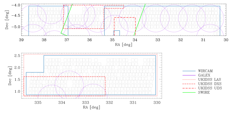
Figure 1: The coverage of ancillary data over the two VIPERS fields (W1 and W4 in the upper and lower panels, respectively). The W1 view is limited to the region sampled by VIPERS until now. Each survey is shown with a different colour (see bottom right legend), while grey quadrants are the VIMOS pointings that led to the spectroscopic catalogue used in this work.

VIPERS is an ongoing redshift survey that aims at observing approximately $100\,000$ galaxies and AGNs at intermediate redshifts ($\langle z\rangle\sim 0.8$) in the magnitude range of $17.5\leqslant i\leqslant 22.5$. At the completion of the survey, expected in 2014, approximately $24$ deg² will have been covered within two fields of the Canada-France-Hawaii Telescope Legacy Survey Wide (CFHTLS-Wide), namely W1 and W4. The sky region covered at present is $\sim 7.5\,{\rm deg}^{2}$ in each of them, with an effective area of $5.34\,{\rm deg}^{2}$ in W1 and $4.97\,{\rm deg}^{2}$ in W4, after accounting for the photometric and spectroscopic masks. Once completed, VIPERS will be the largest spectroscopic survey at such redshifts in terms of volume explored ($1.5\times 10^{8}\,\mathrm{Mpc}^{3}\,h_{70}^{-3}$). All details on the survey design and construction can be found in Guzzo et al. (2013).

The main science drivers of VIPERS are the accurate measurement of galaxy clustering, bias parameter, and the growth rate of structures, along with the study of the statistical properties of galaxies and their evolution when the Universe was about half its current age. These topics are the subject of the parallel accompanying papers of this series (Guzzo et al., 2013; de la Torre et al., 2013; Marulli et al., 2013; Malek et al., 2013; Bel et al., 2013). A previous smaller VIPERS sample has already been used to de-project angular clustering in the CFHTLS full catalogue (Granett et al., 2012) and to develop a galaxy classification through principal component analysis (Marchetti et al., 2013).

The spectroscopic survey is complemented by photometric ancillary data (Fig. 1), obtained from public surveys and dedicated observations, allowing us to estimate several galaxy properties with high precision, in particular galaxy stellar masses and rest-frame magnitudes.

2.1 Photometry

The VIPERS spectroscopic sample has been selected from the W1 and W4 fields of the CFHTLS-Wide. Therefore, for each galaxy we have a photometric dataset consisting of $u^{\ast}$, $g^{\prime}$, $r^{\prime}$, $i^{\prime}$, and $z^{\prime}$ magnitudes (SExtractor’s MAG_AUTO derived in double image mode in order to maintain the same aperture in all bands, Bertin & Arnouts, 1996), as measured by the Terapix team for the T0005 data release (Mellier et al., 2008). The Terapix photometric masks, which discard areas around bright stars or with problematic observations, have been revisited by our team to recover regions within those masks where the photometric quality is deemed sufficient for our analysis (Guzzo et al., 2013).

We took advantage of the full wavelength range of the VIPERS photometric dataset, since this significantly improves the results of our SED fitting; in particular, near-infrared (NIR) fluxes are critical to constraing physical parameters and break degeneracies between the mean age of the stellar population and dust attenuation, and they allow one to compute a robust estimate of stellar masses (e.g. Lee et al., 2009).

To exploit the full potential of VIPERS in analysing the galaxy properties as a function of time and environment, we have undertaken a follow-up in the $K$-band in the two VIPERS fields with the WIRCAM instrument at CFHT and in the far- and near-UV ($FUV$ and $NUV$) channel with the GALEX satellite (Arnouts et al., in prep.). The $K$-band observations were collected between 2010 and 2012 with several discretionary time programmes. The $K$-band depth has been optimised to match the brightness of the spectroscopic sources: at the magnitude limit ($K_{\rm WIRCAM}\simeq 22.0$ at $5\sigma$), $95$% of the spectroscopic sample in W4 is observed in $K_{\rm WIRCAM}$, while in W1 this percentage is approximately $80$% (see Fig. 1).

In addition to WIRCAM data, we matched our CFHTLS optical catalogue with the recent UKIDSS data releases using a matching radius of $0.8\arcsec$. The W1 field overlaps with UDS and DXS, whereas the W4 field is fully covered by the shallower LAS and partially covered by DXS. Where available, we use Petrosian magnitudes in the $Y$, $J$, $H,$ and $K$ bands converted in the AB system. When also considering $K_{\rm UKIDSS}$, the percentage of our spectroscopic sample with $K$-band magnitude increases to $97$% in W1 and $96$% in W4.

We compared the $K$-band photometry for optical sources matched with both UKIDSS and WIRCAM surveys, and find good agreement. In fact, we find a mean difference $\langle\Delta K\rangle=\langle K_{\mathrm{WIRCAM}}-K_{\mathrm{UKIDSS}}\rangle\simeq-0.05$, with a small dispersion $\sigma_{\Delta K}\simeq 0.10$ and $0.15$, for W1 and W4, respectively. These differences can be ascribed to the transmission functions of the filters and the definition of the aperture used when measuring magnitudes, and are close to photometric errors. To not overweight the $K$-band magnitudes in the SED fitting, only the deeper $K_{\mathrm{WIRCAM}}$ data have been used when both magnitudes were available for the same object.

The UV part of the spectrum can also be important for constraining the galaxy dust content and the star formation rate. We make use of existing GALEX images observed with the deep imaging survey (integration time $\sim 3\times 10^{4}$ s) in the $NUV$ and $FUV$ channels, and we have completed the coverage in W1 region with new observations in the $NUV$ channel alone and with integration time $T_{\rm exp}>1.5\times 10^{4}$ s. Because of the GALEX large PSF ($\sim 5$ arcsec), the source blending is a major issue in GALEX deep-imaging mode. To measure the UV fluxes of the sources, we use the dedicated photometric algorithm EMphot (Conseil et al., 2011), which adopts the positions of $U$-band selected priors and performs a modelled PSF adjustment over small tiles based on the expectation maximisation algorithm (Guillaume et al., 2006). For our spectroscopic sample, $63$% ($15$%) of the sources have an $NUV$ ($FUV$) flux measurement in W1. In contrast, the W4 field has modest GALEX coverage: $13$% ($5$%) of spectroscopic sources with an $NUV$ ($FUV$) flux. The WIRCAM and GALEX datasets in the VIPERS fields are described in Arnouts et al. (in prep.).

Moreover, for $\sim 30$% of the spectroscopic targets in W1, we also took advantage of the SWIRE observations in the XMM-LSS field. For our SED fitting we only considered magnitudes in the $3.6\,\mu$m and $4.5\,\mu$m bands, since beyond those wavelengths the survey is shallower, and source detection is very sparse. Moreover, at longer wavelengths the re-emission from dust begins to contribute to the flux of galaxies, and this feature is not reproduced by most of the models of stellar population synthesis (see Sect. 2.3).

2.2 Spectroscopy

The spectroscopic catalogue used in this paper represents the first $60$% of VIPERS. This sample includes $53\,608$ galaxy spectra and will be made available through the future VIPERS Public Data Release 1 (PDR-1). The VIPERS targets were selected via two criteria. The first was aimed at separating galaxies and stars, and relies on the combination of a point-like classification (based on measuring the half-light radius) for the brightest sources and on comparing the five optical magnitudes with galaxy and stellar spectral energy distributions for the faintest ones (Coupon et al., 2009). A fraction of the point-like sources are targeted as AGN candidates, when located in the AGN loci of the two colour diagrams $(g-r)$ versus $(u-g)$ and $(g-i)$ versus $(u-g)$. The second selection criterion, based on $(g-r)$ and $(r-i)$ colours, was applied to exclude low-redshift ($z<0.5$) objects, and has been tested to ensure it does not introduce any significant bias. A complete description of the whole source selection procedure is included in Guzzo et al. (2013).

The spectroscopic observations were carried out using the VIMOS instrument on VLT with the LR-Red grism ($R=210$), giving a wavelength range of $5500$–$9500\,\mathrm{\AA}$ that guarantees the observability of the main spectral features in the VIPERS redshift range, e.g. the absorption lines CaII H & K $\lambda\lambda 3934,3969$ and the emission line [OII] $\lambda 3727$. Using a sample of objects spectroscopically observed twice, we are able to estimate an uncertainty of $\sigma_{z}=0.00047\,(1+z)$ for our measured redshifts.

To maximise the multiplex capability of VIMOS, we adopted the observational strategy described in Scodeggio et al. (2009) of using shorter slits than in the previous surveys carried out with the same instrument. By virtue of this strategy, we reached a sampling rate of approximately $40$% with a single pass, essential to estimating the large-scale environment (Cucciati et al., in prep.; Iovino et al., in prep.).

The spectroscopic masks reproduce the footprint of the VIMOS instrument, consisting of four quadrants and gaps between them for each pointing, covering $224\,{\rm arcmin}^{2}$. Vignetted parts of the quadrants have been removed to compute the effective area (for a detailed description see Guzzo et al., 2013).

Data reduction and redshift measurement were performed within the software environment Easylife (Garilli et al., 2012), which is based on the VIPGI pipeline (Scodeggio et al., 2005) and EZ (Garilli et al., 2010, Easy redshift). Once measured by the EZ pipeline and assigned a confidence level, the spectroscopic redshifts were then checked and validated independently by two team members. In case of any discrepancy, they were reconciled by direct comparison. In the vast majority of cases, this involves spectra with very low signal-to-noise ratios, which end up in the lowest quality classes. In general, each redshift is in fact assigned a confidence level, based on a well-established scheme developed by previous surveys like VVDS (Le Fèvre et al., 2005) and zCOSMOS (Lilly et al., 2009). In detail, a spectroscopic quality flag equal to $4$ corresponds to a confidence level of $99.6$%, with smaller flags corresponding to lower confidence levels, as described in (Guzzo et al., 2013). Objects with a single emission line are labelled by flag $9$, and broad-line AGNs share the same scheme, but their flags are increased by $10$. Each spectroscopic flag also has a decimal digit specifying the agreement with the photometric redshift computed from CFHTLS photometry (Coupon et al., 2009).

After excluding $3\,394$ galaxies with no redshift measurement (flag $0$, which represents the lack of a reliable redshift estimate) and $1\,750$ stars, our redshift sample contains $53\,608$ extragalactic sources, nearly equally split between the two fields. The quality of redshift measurements for the sample with spectroscopic flags larger than $2$, as estimated from the validation of multiple observations, is high (confidence $>95\%$, see Guzzo et al., 2013).

Since only a fraction of all the possible targets have been observed, statistical weights are required to make this subsample representative of all the galaxies at $i\leqslant 22.5$ in the survey volume. Such weights are calculated by considering the number of photometric objects that have been targeted (target sampling rate, TSR), the fraction of them classified as secure measurements (spectroscopic success rate, SSR), and the completeness due to the colour selection (colour sampling rate, CSR). The statistical weights can depend on the magnitude, redshift, colour, and angular position of the considered object. For each part of the statistical weight we considered only the main and relevant dependencies, in order to avoid spurious fluctuations when there are small subsamples. In particular, we considered the TSR as a function of only the selection magnitude, the SSR as a function of magnitude and redshift, and the CSR (estimated by using data from the VVDS flux limited survey, Le Fèvre et al., 2005) as a function of redshift. Regarding the SSR, only galaxies with quality flags between $2$ and $9$ ($\sim 41\,100$ galaxies in the redshift range $0.5\leqslant z\leqslant 1.3$) were considered in the analysis. (We exclude spectra classified as broad-line AGNs.) For a galaxy at redshift $z$ with magnitude $i$, its statistical weight $w(i,z)$ is the inverse of the product of TSR($i$), SSR($i,z$), and CSR($z$). Once each galaxy in the spectroscopic sample is properly weighted, we can recover the properties of the photometric parent sample with good precision (for a detailed discussion on TSR, SSR, and CSR see Guzzo et al., 2013).

2.3 Stellar masses

Figure 2: Distribution of the differences between the values of stellar mass estimated using the two codes Hyperzmass and MAGPHYS. Only results for the W1 field are shown (see text). To limit the effects of parameter degeneracy, we restrict the comparison to galaxies that turn out to have solar metallicity, according to their best-fit templates both in Hyperzmass and MAGPHYS. In this way the difference between $\mathcal{M}_{\mathrm{MAGPHYS}}$ and $\mathcal{M}_{\mathrm{Hyperzmass}}$ cannot be due to a different metal content assumed in the two SED fitting estimates. The dashed line gives the best-fitting Gaussian of the distribution, corresponding to the mean and standard deviation indicated. Also indicated are the size of the galaxy subsample ($N_{\mathrm{tot}}$) and the number of stellar mass estimates for which the discrepancy is $\log(\mathcal{M}_{\mathrm{MAGPHYS}}/\mathcal{M}_{\mathrm{Hyperzmass}})>2\sigma$ ($N_{\mathrm{exceed}}$).

Considering the small fraction of objects without $K$ band magnitude, we decided to rely on SED fitting to derive stellar masses and to not implement alternative methods, such as the Lin et al. (2007) relation between stellar mass, redshift, and rest-frame magnitudes.

We thus derive galaxy stellar masses by means of an updated version of Hyperzmass (Bolzonella et al., 2000, 2010, software is available on request). Given a set of synthetic spectral energy distributions, the software fits these models to the multi-band photometry for each galaxy and selects the model that minimises the $\chi^{2}$. The SED templates adopted in this procedure are derived from simple stellar populations (SSPs) modelled by Bruzual & Charlot (Bruzual & Charlot, 2003, hereafter BC03), adopting the Chabrier (2003) universal initial mass function (IMF) . The BC03 model is one of the most commonly used ones (e.g. Ilbert et al., 2010; Zahid et al., 2011; Barro et al., 2013). Another frequently used SSP library is the one by Maraston (2005, M05), which differs from the former because of the treatment of the thermally pulsing asymptotic giant branch (TP-AGB) stellar phase, affecting NIR emission of stellar populations aged $\sim 1\,{\rm Gyr}$. The question about the relevance of TP-AGB in the stellar population synthesis is still open (e.g. Marigo & Girardi, 2007), with some evidence that supports BC03 (Kriek et al., 2010; Zibetti et al., 2013) in contrast to observations favouring M05 (MacArthur et al., 2010). In the following we prefer to adopt the BC03 model, since most of the galaxies in the redshift range we consider should not be dominated by the TP-AGB phase (which is instead relevant for galaxies at $1.4\leqslant z\leqslant 2.7$, Maraston et al., 2006).

The SSPs provided by Bruzual & Charlot (2003) assume a non-evolving stellar metallicity $Z$, which we chose to be solar ($Z=Z_{\odot}$) or subsolar ($Z=0.2\,Z_{\odot}$). This choice allows us to take the different metallicities of the galaxies in our redshift range into account, which can be lower than in the nearby universe (Zahid et al., 2011), without significantly increasing the effect of the age-metallicity degeneracy. Considering the low resolution of our spectroscopic setup, it is difficult to put reliable constraints on $Z$ from the observed spectral features, and therefore it was not possible to constrain this parameter a priori. Therefore, the metallicity assigned to each galaxy is what is obtained from the best-fit model (smallest $\chi^{2}$).

With respect to the galaxy dust content, we implemented the Calzetti et al. (2000) and Prévot-Bouchet (Prevot et al., 1984; Bouchet et al., 1985) extinction models, with values of $A_{V}$ ranging from $0$ (no dust) to $3$ magnitudes. As pointed out in previous work (e.g. Inoue, 2005; Caputi et al., 2008; Ilbert et al., 2009), Calzetti’s law is on average more suitable for the bluest SEDs, having been calibrated on starburst (SB) galaxies, whereas the Prévot-Bouchet law is better for mild star-forming galaxies, since it was derived from the dust attenuation of the Small Magellanic Cloud (SMC) (see also Wuyts et al., 2011). Hereafter we refer to the Calzetti and Prévot-Bouchet models as SB and SMC extinction laws, respectively. We let the choice between the two extinction laws be free, according to the best-fit model (smallest $\chi^{2}$), since we do not have sufficient data at UV wavelengths to differentiate the different trends of the two laws.

The SEDs constituting our template library are generated from the SSPs following the evolution described by a given star formation history (SFH). In this work, we assume exponentially declining SFHs, for which $\mathrm{SFR}\propto\exp(-t/\tau)$, with the time scale $\tau$ ranging from $0.1$ to $30\,\mathrm{Gyr}$. A constant SFH (i.e., $\mathrm{SFR}\sim 1\,\mathcal{M}_{\odot}\,\mathrm{yr}^{-1}$) is also considered. This evolution follows unequally spaced time steps, from $t=0$ to $t=20\,\mathrm{Gyr}$. No fixed redshift of formation is imposed in this model.

Although such a parametrisation is widely used, recent studies have shown how exponentially increasing SFHs can provide a more realistic model for actively star-forming galaxies in which young stellar populations outshine the older ones (Maraston et al., 2010). This effect becomes relevant at $z\sim 2$, when the cosmic star formation peaks, and can be reduced by setting a lower limit on the age parameter, in order to avoid unrealistic solutions that are too young and too dusty (Pforr et al., 2012). In our redshift range, galaxies whose SFH rises progressively have low stellar masses ($\log(\mathcal{M}/\mathcal{M_{\odot}})\sim 9.5$, Pacifici et al., 2013) falling below the limit of VIPERS. Moreover, Pacifici et al. (2013) identify a class of massive blue galaxies that assembled their stellar mass over a relatively long period, experiencing a progressive reduction of their star formation at a later evolutionary stage. For such bell-shaped SFH, neither increasing nor decreasing $\tau$-models seem to be suitable. However, the resulting differences are smaller than the other uncertainties of the SED fitting method (cf. Conroy et al., 2009).

Another issue concerning the SFH is the assumption of smoothness. In fact, a galaxy could have experienced several phases of intense star formation during its past, which can be taken into account by superimposing random peaks on the exponential (or constant) SFR (Kauffmann et al., 2003a). Allowing the presence of recent secondary bursts, thereby making the colours of an underlying old and red population bluer, can lead to a systematically higher stellar mass estimate. However, only for a small fraction of objects is the difference in $\mathcal{M}$ larger than $0.2$ dex, as shown by Pozzetti et al. (2007).

We also quantified the effect of using complex SFHs in VIPERS, by computing stellar masses using the MAGPHYS package (da Cunha et al., 2008). This code parametrises the star formation activity of each galaxy template starting from the same SSP models as Hyperzmass (i.e., BC03), but using two components in the SFH, namely an exponentially declining SFR and a second component of additional bursts randomly superimposed on the former according to Kauffmann et al. (2003a). The probability of a secondary burst occurring is such that half of the galaxy templates in the library have experienced a burst in their last $2\,\mathrm{Gyr}$. Each of those episodes can last $3\times 10^{7}$–$3\times 10^{8}\,$yr, producing stars at a constant rate. The ratio between the stellar mass produced in a single burst and the one formed over the entire galaxy’s life by the underlying exponentially declining model is distributed logarithmically between $0.03$ and $4.0$. The dust absorption model adopted in MAGPHYS is the one proposed by Charlot & Fall (2000), which considers the optical depth of H II and H I regions embedding young stars along with the extinction caused by diffuse interstellar medium. MAGPHYS treats attenuation in a consistent way, including dust re-emission at infrared wavelengths; however, this feature does not represent a significant advantage when dealing with VIPERS data since infrared magnitudes are too sparse in our catalogue. Metallicity values are distributed uniformly between $0.02$ and $2\,Z_{\odot}$. The wide range of tightly sampled metallicities, the different model for the dust extinction, and in particular the complex SFHs in the MAGPHYS library are the major differences with respect to the Hyperzmass code.

In Fig. 2 we compare the estimates obtained through MAGPHYS and Hyperzmass, and verify that complex SFHs have a minimal impact on the results (see Sect. 3.4). Since MAGPHYS requires a much longer computational time than other SED fitting codes, we only estimate the stellar mass for galaxies in the W1 field between $z=0.5$ and $z=1.3$. Moreover, for this comparison we selected objects with the same (solar) metallicity in both the SED fitting procedures, because in this way we are able to investigate the bias mainly thanks to the different SFH parametrisations. The distribution of the ratio between the two mass estimates is reproduced well by a Gaussian function plus a small tail towards positive values of $\log(\mathcal{M}_{\mathrm{MAGPHYS}}/\mathcal{M}_{\mathrm{Hyperzmass}})$. We find a small offset ($\langle\Delta\log\mathcal{M}\rangle=\langle\log(\mathcal{M}_{\mathrm{MAGPHYS}}/\mathcal{M}_{\mathrm{Hyperzmass}})\rangle\simeq 0.05$) and a small dispersion ($\sigma_{\Delta\mathcal{M}}\simeq 0.11$) for most of the galaxy population, with significant differences between MAGPHYS and Hyperzmass (i.e., $\Delta\log\mathcal{M}>0.22$) for only $\sim 7$% of the testing sample ($N_{\mathrm{exceed}}$ in Fig. 2). The consequences on the GSMF are discussed in Sect. 3.4.

Given the wide range of physical properties allowed in the SED fitting procedure, we decided to exclude some unphysical parameter combinations from the fitting. In particular, we limit the amount of dust in passive galaxies (i.e., we impose $A_{V}\leqslant 0.6$ for galaxies with ${\rm age}/\tau>4$), we avoid very young extremely star-forming galaxies with short $\tau$ timescales (i.e. we prevent fits with models with $\tau\leqslant 0.6\,{\rm Gyr}$ when requiring $z_{\rm form}<1$), and we only allow ages to be within $0.1$ Gyr and the age of the Universe at the spectroscopic redshift of the fitted galaxy (see Pozzetti et al., 2007; Bolzonella et al., 2010).

According to Conroy et al. (2009), the uncertainties associated with the SED fitting can be $\sim 0.3$ dex when considering all the possible parameters involved and their allowed ranges. In particular, given the non-uniform coverage of the GALEX and SWIRE ancillary data matched with our sample, we checked that the variation in the magnitude set from one object to another does not introduce significant bias. For the subsample of galaxies with $FUV$, $NUV$, $3.6\,\mu$m, and $4.5\,\mu$m bands available, we also estimate the stellar mass using just the optical-NIR photometry. We find no systematic difference in the two estimates of stellar mass (with and without the UV and infrared photometry) and only a small dispersion of about $0.08$ dex.

In summary, the VIPERS galaxy stellar mass estimates are obtained using the BC03 population synthesis models with Chabrier IMF, smooth (exponentially declining or constant) SFHs, solar and subsolar metallicity, and the SB and SMC laws for modelling dust extinction. Unless stated otherwise, this is the default parametrisation used throughout this paper.

3 From stellar masses to the galaxy stellar mass function

In this section we exploit the VIPERS dataset described above by considering only our fiducial sample of $41\,094$ galaxies at $z=[0.5,1.3]$ with spectroscopic redshift reliability $>95$% (see Sect. 2.2). As mentioned above, broad-line AGNs ($\sim 850$ in the present spectroscopic sample) are naturally excluded from the sample, being visually identified during the redshift measurement process. Instead, narrow-line AGNs are not removed from our sample, but they do not constitute a problem for the SED fitting derived properties, since in most of the cases their optical and NIR emission are dominated by the host galaxy (Pozzi et al., 2007). First of all, we try to identify the threshold above which the sample is complete, and therefore the mass function can be considered reliable. After that, we derive the GSMF of VIPERS in various redshift bins and discuss the main sources of uncertainty affecting it.

3.1 Completeness

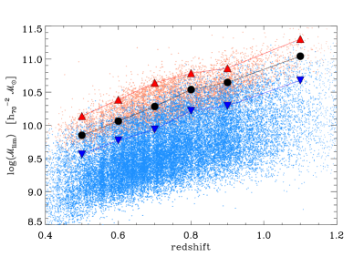
Figure 3: The mass completeness threshold $\mathcal{M}_{\mathrm{lim}}$ as a function of redshift, computed for the total sample (the one used in Sect. 3.2, filled circles) and for the red (upward triangles) and blue (downward triangles) populations, defined as discussed in Sect. 5. In each redshift bin, the $\mathcal{M}_{\mathrm{lim}}$ estimate relies on the rescaled stellar mass $\mathcal{M}(i=i_{\mathrm{lim}})$ of the $20$% faintest galaxies (see text). We show $\mathcal{M}(i=i_{\mathrm{lim}})$ of the red and blue galaxies with small dots of analogous colours.

In the literature, the completeness mass limit of a sample at a given redshift is often defined as the highest stellar mass a galaxy could have, when its observed magnitude matches the flux limit (e.g. Pérez-González et al., 2008). This maximum is usually reached by the rescaled SED of an old passive galaxy. However, this kind of estimate gives rise to a threshold that tends to be too conservative. The sample incompleteness is due to galaxies that can be potentially missed, because their flux is close to the limit of the survey. Depending on the redshift, such a limit in apparent magnitude can correspond to faint luminosities; in that case, only a small fraction of objects will have a high stellar mass-to-light ratio, since blue galaxies (with lower $\mathcal{M}/L$) will be the dominant population (e.g. Zucca et al., 2006). Thus, if based on the SED of an old passive galaxy, the determination of the stellar mass completeness is somehow biased in a redshift range that depends on the survey depth (see also the discussion in Marchesini et al., 2009, Appendix C).

To avoid this problem, we apply the technique devised by Pozzetti et al. (2010). This procedure yields, for a given redshift and flux limit, an estimate of the threshold $\mathcal{M}_{\mathrm{lim}}$ below which some galaxy type cannot be detected any longer. Following this approach, we estimate the stellar mass each object would have if its magnitude, at the observed redshift, were equal to the $i$-band limiting magnitude $i_{\mathrm{lim}}$. This boundary mass $\mathcal{M}(i\!=\!i_{\mathrm{lim}})$ is obtained by rescaling the original stellar mass of the source at its redshift, i.e. $\log\mathcal{M}(i\!=\!i_{\mathrm{lim}})=\log\mathcal{M}+0.4(i-i_{\mathrm{lim}})$. The threshold $\mathcal{M}_{\mathrm{lim}}$ is then defined as the value above which $90$% of the $\mathcal{M}(i\!=\!i_{\mathrm{lim}})$ distribution lies. According to this, at values higher than $\mathcal{M}_{\mathrm{lim}}$, our GSMF can be considered complete. We include in the computation only the $20$% faintest objects to mitigate the contribution of bright red galaxies with large $\mathcal{M}/L$ when they are not the dominant population around the flux limit, as they may cause the bias discussed at the beginning of this section.

Since the $1/V_{\mathrm{max}}$ method (Schmidt, 1968, see Sect. 3.2) intrinsically corrects the sample incompleteness above the lower limit of the considered redshift bin ($z_{\mathrm{inf}}$), we apply to each redshift bin the $\mathcal{M}_{\mathrm{lim}}$ computed by considering the objects inside a narrow redshift interval $\Delta z=0.05$ centred on $z_{\mathrm{inf}}$. Figure 3 shows $\mathcal{M}_{\mathrm{lim}}$ as a function of redshift for the global and for the red and blue samples used in Sect. 5, as well as the value of $\mathcal{M}(i\!=\!i_{\mathrm{lim}})$ for each red and blue galaxy. As expected, the limiting mass increases as a function of $z$ and the values for red galaxies are significantly higher ($\sim 0.5\,\mathrm{dex}$) than for the blue ones.

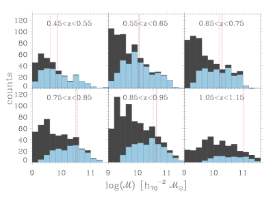
Figure 4: Distributions of stellar masses in six redshift bins for the VVDS-Deep sample in the CFHTLS-W1 field at its limiting magnitude ($I\leqslant 24$, dark histograms), compared to the subset obtained by applying a magnitude cut similar to VIPERS, at $I\leqslant 22.5$ (blue histograms). In each panel, the black dashed line represents the limiting mass for the VVDS sample with $I\leqslant 22.5$. The red solid line instead gives the limiting mass for the VIPERS sample in the W1 field. Both limits, in good agreement with each other, correctly identify the threshold below which the shallower sample starts to miss a significant fraction ($>20\%$) of objects.

In the context of the zCOSMOS project (Lilly et al., 2009), the approach of Pozzetti et al. (2010) produced completeness limits in good agreement with those obtained through mock survey samples (Meneux et al., 2009). In VIPERS, we successfully tested our $\mathcal{M}_{\mathrm{lim}}$ estimates by taking advantage of the VVDS-Deep field, which is located in the W1 field (see Guzzo et al., 2013, Fig. 2). The VVDS sample provides us with spectroscopically observed galaxies down to a fainter limit, i.e. $I_{\rm AB}=24$ (Le Fèvre et al., 2005). Since the CFHTLS-W1 field contains both VVDS and part of VIPERS, we can compare the stellar masses by relying on a similar photometric baseline $(u,g,r,I,i,z,J^{*},K^{*})$. When applying a VIPERS-like magnitude cut ($I<22.5$), we can find the fraction of missed objects with respect to the parent $I<24$ sample as a function of stellar mass. This test is shown in Fig. 4, where we compare the $\mathcal{M}_{\mathrm{lim}}$ values of VVDS (limited to $I\leqslant 22.5$) and VIPERS to the distribution of stellar masses belonging to the deeper (i.e., $I\leqslant 24$) VVDS sample. The $\mathcal{M}_{\mathrm{lim}}$ values we computed are close to the thresholds at which the stellar mass distribution starts to be incomplete with respect to the deep VVDS sample (i.e. the limit where the $I<22.5$ sample recovers less than $80$% of the parent sample).

3.2 Evolution of the mass function for the global population

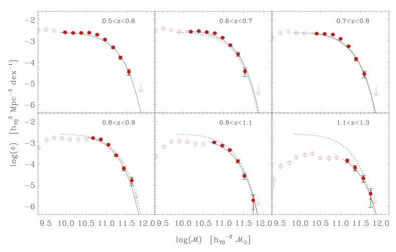
Figure 5: The VIPERS galaxy stellar mass function at different redshifts. Circles give the values determined through $1/V_{\mathrm{max}}$ in mass bins of $\Delta\mathcal{M}=0.2$ dex; the centre of each bin corresponds to the weighted mean mass of the objects within it. Empty and filled symbols correspond to values below and above the completeness limit, respectively (see Sect. 3.1). For the latter points, the red error bars show the uncertainty due to Poisson noise, while green bars account for Poisson noise and cosmic variance. In each panel, a solid line shows the Schechter best-fit to the GSMF filled points, with the dashed line reproducing that of the first redshift bin, as a reference. The downward arrows give an upper limit to $\Phi$ where no detection is available.

The number of galaxies and the volume sampled by VIPERS allows us to obtain an estimate of the GSMF with high statistical precision within six redshifts bins in the range $0.5\leqslant z\leqslant 1.3$. Given the large number of galaxies observed by VIPERS, in terms of Poisson noise it would be possible to choose even narrower bins (e.g. $\Delta z\simeq 0.05$ wide). However, in that case the measurements start being strongly affected by cosmic (sample) variance. A more detailed discussion is given in Sect. 3.3.

We compute the GSMF within each redshift bin, using the classical non-parametric $1/V_{\mathrm{max}}$ estimator (Schmidt, 1968). With this method, the density of galaxies in a given stellar mass bin is obtained as the sum of the inverse of the volumes in which each galaxy would be observable, multiplied by the statistical weight described in Sect. 2.2. To optimise the binning in stellar mass, we use an adaptive algorithm that extends the width of a bin until it contains a minimum of three objects. The errors associated with the $1/V_{\mathrm{max}}$ estimates are computed assuming Poisson statistics and include statistical weights. The upper limits for non-detections have been estimated following Gehrels (1986). The values of the $1/V_{\mathrm{max}}$ GSMF and associated Poisson errors are given in Table 1.

It is well known that the $1/V_{\mathrm{max}}$ estimator is unbiased in case of a homogeneous distribution of sources (Felten, 1976), but it is affected by the presence of clustering (Takeuchi et al., 2000). At variance with the data sets on which the estimator was tested in the past, VIPERS has a specific advantage, thanks to its large volume over two independent fields. The competing effects of over- and under-dense regions on the estimate should cancel out in such a situation. The impact on our analysis will also be negligible because an inhomogeneous distribution of sources mainly affects the faint end (i.e. the low mass end) of the luminosity (stellar mass) function (Takeuchi et al., 2000), while we are mainly interested in the massive tail of the distribution.

To verify this, we compare the $1/V_{\mathrm{max}}$ estimates with those of a different estimator (i.e. the stepwise maximum-likelihood method of Efstathiou et al., 1988) from another software package (ALF, Ilbert et al., 2005). We find no significant differences in the obtained mass functions, within the stellar mass range considered in the present study.

Finally, in addition to the non-parametric method, we fit a Schechter (1976) function, that is,

$$\Phi(\mathcal{M})\mathrm{d}\mathcal{M}=\Phi_{\star}\left(\frac{\mathcal{M}}{\mathcal{M}_{\star}}\right)^{\alpha}\exp\left(-\frac{\mathcal{M}}{\mathcal{M}_{\star}}\right)\frac{\mathrm{d}\mathcal{M}}{\mathcal{M}_{\star}}\>,$$ (1)

to the $1/V_{\mathrm{max}}$ estimates. The results are shown in Fig. 5 and in Table 2. Although the mass function does not show any evidence of a rapid decline below the completeness limit (as in Drory et al., 2009), points beyond this threshold should be considered as conservative lower limits. These plots clearly show the statistical power of the VIPERS sample, which includes a significant number of the rare massive galaxies that populate the GSMF high-mass end, thanks to its large volume.

Figure 6: Evolution of the galaxy number density in different bins of stellar mass. The error bars of the density estimates include Poisson noise and cosmic variance (see Sect. 3.3). At $z\simeq 1.2$, for the lowest mass sample, only a lower limit can be estimated, indicated by the arrow.

At $z<0.6$ there is some hint of the characteristic dip of the mass function at $\log(\mathcal{M}/\mathcal{M}_{\odot})\sim 10.2$, with an upturn below that value as observed both locally (e.g. Baldry et al., 2012) and at intermediate redshifts (e.g Drory et al., 2009; Pozzetti et al., 2010). However, this feature is located too close to $\mathcal{M}_{\mathrm{lim}}$ to be assessed effectively. We avoid using a double Schechter function in our fits also to ease comparison with the parameters derived at higher redshifts. In fitting the points in the first bin ($0.5<z<0.6$), all parameters of Eq. 1 are left free, obtaining a value of the slope $\alpha=-0.95$. Above this redshift, however, the slope of the low-mass end is only weakly constrained, given the relatively high values of the completeness limit $\mathcal{M}_{\mathrm{lim}}$. For this reason, in all the other bins we fix $\alpha$ to the value $-0.95$ (see Table 2).

Table 1: Global GSMF: $1/V_{\rm max}$ values in regular bins of stellar mass.

$\log\mathcal{M}\;[h_{70}^{-2}\,\mathcal{M}_{\odot}]$	$\log\Phi\;[h_{70}^{3}\,\mathrm{Mpc}^{-3}]$
	$0.5<z<0.6$	$0.6<z<0.7$	$0.7<z<0.8$	$0.8<z<0.9$	$0.9<z<1.1$	$1.1<z<1.3$
$9.50$	$-2.47^{+0.02}_{-0.02}$	$-2.42^{+0.01}_{-0.02}$	$-2.62^{+0.02}_{-0.02}$	$-2.89^{+0.03}_{-0.03}$	$-3.20^{+0.04}_{-0.04}$	$-4.11^{+0.11}_{-0.15}$
$9.70$	$-2.51^{+0.02}_{-0.02}$	$-2.49^{+0.01}_{-0.01}$	$-2.56^{+0.02}_{-0.02}$	$-2.78^{+0.02}_{-0.02}$	$-2.95^{+0.03}_{-0.03}$	$-3.95^{+0.07}_{-0.08}$
$9.90$	$-2.61^{+0.02}_{-0.02}$	$-2.56^{+0.02}_{-0.02}$	$-2.63^{+0.02}_{-0.02}$	$-2.79^{+0.03}_{-0.03}$	$-2.93^{+0.03}_{-0.03}$	$-3.69^{+0.06}_{-0.07}$
$10.10$	$-2.67^{+0.02}_{-0.02}$	$-2.59^{+0.02}_{-0.02}$	$-2.65^{+0.02}_{-0.02}$	$-2.84^{+0.02}_{-0.02}$	$-2.98^{+0.03}_{-0.03}$	$-3.58^{+0.07}_{-0.08}$
$10.30$	$-2.68^{+0.02}_{-0.02}$	$-2.59^{+0.01}_{-0.01}$	$-2.69^{+0.02}_{-0.02}$	$-2.85^{+0.02}_{-0.02}$	$-3.07^{+0.03}_{-0.03}$	$-3.53^{+0.06}_{-0.07}$
$10.50$	$-2.66^{+0.02}_{-0.02}$	$-2.62^{+0.01}_{-0.01}$	$-2.70^{+0.02}_{-0.02}$	$-2.85^{+0.02}_{-0.02}$	$-3.07^{+0.03}_{-0.03}$	$-3.73^{+0.05}_{-0.05}$
$10.70$	$-2.72^{+0.02}_{-0.02}$	$-2.67^{+0.01}_{-0.01}$	$-2.75^{+0.01}_{-0.02}$	$-2.83^{+0.02}_{-0.02}$	$-3.04^{+0.02}_{-0.02}$	$-3.74^{+0.10}_{-0.13}$
$10.90$	$-2.91^{+0.02}_{-0.02}$	$-2.81^{+0.02}_{-0.02}$	$-2.83^{+0.02}_{-0.02}$	$-2.97^{+0.02}_{-0.02}$	$-3.16^{+0.02}_{-0.02}$	$-3.71^{+0.06}_{-0.07}$
$11.10$	$-3.25^{+0.03}_{-0.03}$	$-3.11^{+0.02}_{-0.02}$	$-3.14^{+0.02}_{-0.02}$	$-3.26^{+0.02}_{-0.03}$	$-3.32^{+0.02}_{-0.03}$	$-3.93^{+0.07}_{-0.09}$
$11.30$	$-3.66^{+0.05}_{-0.05}$	$-3.55^{+0.04}_{-0.04}$	$-3.59^{+0.04}_{-0.04}$	$-3.83^{+0.04}_{-0.05}$	$-3.81^{+0.04}_{-0.04}$	$-4.13^{+0.09}_{-0.12}$
$11.50$	$-4.34^{+0.09}_{-0.12}$	$-4.22^{+0.07}_{-0.09}$	$-4.29^{+0.07}_{-0.09}$	$-4.54^{+0.09}_{-0.12}$	$-4.39^{+0.07}_{-0.08}$	$-4.65^{+0.11}_{-0.15}$
$11.70$	$-5.29^{+0.23}_{-0.53}$	$-5.69^{+0.30}_{{\rm-inf}}$	$-5.05^{+0.16}_{-0.26}$	$-5.19^{+0.18}_{-0.30}$	$-5.78^{+0.23}_{-0.54}$	$-5.20^{+0.14}_{-0.21}$

The results of Fig. 5 confirm, with impressive statistical precision, the lack of evolution since $z\simeq 1.1$ of the massive end ($\log(\mathcal{M}/\mathcal{M}_{\odot})>11$) of the galaxy mass function seen in previous, smaller samples. The exponential tail of the Schechter fit is nearly constant across the five redshift bins, down to $z\simeq 0.5$ (see Fig. 5). However, we detect a significant decrease in the number density of the most massive galaxies ($\log(\mathcal{M/M}_{\odot})>11.1$) in the redshift bin $z=1.1<z<1.3$. At lower masses ($10.8<\log(\mathcal{M}/\mathcal{M}_{\odot})<11.1$), the first signs of evolution with respect to $z\sim 0.5$ start to be visible at redshift $0.9$ – $1.1$.

These trends are shown better in Fig. 6, where the number density of galaxies $\rho_{N}$ within three mass ranges is plotted versus redshift. This figure explicitly shows that the most massive galaxies are virtually already in place at $z\simeq 1$. In contrast, galaxies with lower mass keep assembling their stars in such a way that their number density increases by a factor $\sim 3.5$ from $z=1.2$ down to $0.6$, consistently with the so-called downsizing scenario (Cowie et al., 1996; Fontanot et al., 2009). These new measurements confirm previous evidence, but with higher statistical reliability (see Sect. 4).

Table 2: Global GSMF: Schechter parameters ($\alpha$ fixed at $z>0.6$).

$z$ range	$\alpha$	$\log\mathcal{M}_{\star}$	$\Phi_{\star}$
		$[h_{70}^{-2}\,\mathcal{M}_{\odot}]$	$[10^{-3}\,h_{70}^{3}\,\mathrm{Mpc}^{-3}]$
$0.5-0.6$	$-0.95^{+0.03}_{-0.02}$	$10.87^{+0.02}_{-0.02}$	$1.42^{+0.06}_{-0.07}$
$0.6-0.7$	$-0.95$	$10.91^{+0.02}_{-0.01}$	$1.58^{+0.05}_{-0.05}$
$0.7-0.8$	$-0.95$	$10.91^{+0.01}_{-0.02}$	$1.38^{+0.06}_{-0.04}$
$0.8-0.9$	$-0.95$	$10.85^{+0.02}_{-0.02}$	$1.29^{+0.09}_{-0.09}$
$9.0-1.1$	$-0.95$	$10.91^{+0.02}_{-0.01}$	$0.82^{+0.05}_{-0.06}$
$1.1-1.3$	$-0.95$	$11.03^{+0.11}_{-0.08}$	$0.20^{+0.05}_{-0.06}$

3.3 Cosmic variance in the VIPERS survey

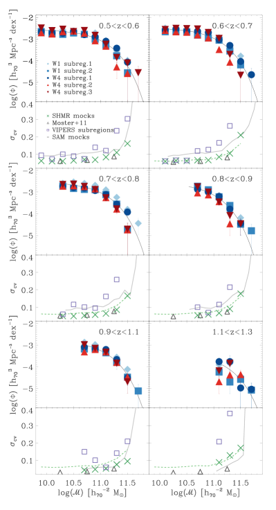
Figure 7: Estimates of the contribution of sample (cosmic) variance to the statistical uncertainty of the GSMF measurements. For each redshift bin, the upper panels show the GSMF $1/V_{\mathrm{max}}$ measurements obtained from five VIPERS subregions of $2\,\mathrm{deg}^{2}$, located respectively in the W1 field (three regions, blue diamonds, circles, and squares) and in the W4 field (two regions, red triangles, and downward triangles). The Schechter fit to the global GSMF of Fig. 5 is shown as reference (black solid line). The lower panels show the standard deviations estimated in each redshift bin from these five measurements (purple squares, Eq. 3), together with the estimates of $\sigma_{\mathrm{cv}}$ obtained from $57$ SHMR mocks by means of Eq. 2 (green crosses). To highlight how the effect of cosmic variance decreases at higher $z$, we report $\sigma_{\mathrm{cv,SHMR}}$ of the first redshift bin in the other panels (green dashed lines). In addition, the sample variance measured in $50$ SAM mocks (grey solid line) and the estimates provided by Moster et al. (2011) method (black triangles) are shown as reference.

When dealing with statistical studies using number counts, a severe complication is introduced by the field-to-field fluctuations in the source density, due to the clustered nature of the galaxy distribution and the existence of fluctuations on scales comparable to the survey volume. This sampling or ‘cosmic’ variance represents a further term of uncertainty to be added to the Poisson shot noise. It can be expressed by removing $\sigma_{\mathrm{Poiss}}^{2}\equiv 1/\langle N\rangle$ from the total relative error:

$$\sigma_{\mathrm{cv}}^{2}=\frac{\langle N^{2}\rangle-\langle N\rangle^{2}}{\langle N\rangle^{2}}-\frac{1}{\langle N\rangle},$$ (2)

where $\langle N\rangle$ and $\langle N^{2}\rangle$ are the mean and the variance of galaxy number counts (Somerville et al., 2004).

Extragalactic pencil-beam surveys, even the deepest ones, are particularly limited by cosmic variance, given the small volume covered per redshift interval. At $z\sim 0.8$, galaxy density fluctuations are found to be still relevant up to a scale of $\sim 140\,{\rm Mpc}\,h_{70}^{-1}$ (Scrimgeour et al., 2012), which roughly corresponds to $5\,\mathrm{deg}$.

This is the result of intrinsic clustering in the matter, as predicted by the power spectrum shape and amplitude at that epoch, amplified by the bias factor of the class of galaxies analysed, which at high redshift can be very large for some classes. Also the last-generation, largest deep surveys are significantly affected by this issue. For example, the COSMOS field, despite its $2\,\mathrm{deg}^{2}$ area, turned out to be significantly overly dense between $z=0.8$ and $z=1$ (Kovač et al., 2010).

The gain obtained by enlarging the area of a single field beyond a certain coverage becomes less prominent, owing to the existing large-scale correlations (see Newman & Davis, 2002, Fig. 1): $\sigma_{\mathrm{cv}}$ decreases mildly as a function of volume, with an approximate dependence $\sigma_{\mathrm{cv}}\propto V^{-0.3}$ (Somerville et al., 2004, Fig. 2), compared to $\sigma_{\mathrm{Poiss}}\propto V^{-0.5}$. Trenti & Stiavelli (2008) found similar results by characterizing Lyman break galaxies surveys: at high values of $\langle N\rangle$, the Poisson noise rapidly drops and cosmic variance remains the dominant source of uncertainty. A more effective way to abate cosmic variance is to observe separated regions of sky. Since counts in these regions, if they are sufficiently distant, are uncorrelated, their variances sum up in quadrature (i.e., $\sigma_{\mathrm{cv}}$ decreases as the square root of the number of fields, Moster et al., 2011). Multiple independent fields can then result in a smaller uncertainty than for a single field, even if the latter has a larger effective area (Trenti & Stiavelli, 2008). The current VIPERS PDR-1 sample is not only characterised by a significantly large area, compared to previous similar surveys at these redshifts, but it is also split into two independent and well-separated fields of $\sim 7.5\,\mathrm{deg}^{2}$ each. We therefore expect that the impact of cosmic variance should be limited.

To quantify this effect directly, we follow two approaches. The first one, based on the observations themselves, provides an upper limit of the VIPERS $\sigma_{\mathrm{cv}}$. We select five rectangular subregions of about $2\,\mathrm{deg}^{2}$ within the survey and estimate the mass function $\Phi_{i}$ in each of them, using the $1/V_{\mathrm{max}}$ method described above. We choose non-contiguous regions (separated by $\sim 1\,\mathrm{deg}$) to minimise the covariance between subsamples located within the same field (W1 or W4). Within mass bins $\mathcal{M}_{j}\pm\Delta\mathcal{M}/2$ we derive the total random uncertainty

$$\sigma_{\mathrm{tot,obs}}(\mathcal{M}_{j})=\frac{1}{n}\sum_{i=1}^{n}\sqrt{\left[\Phi_{i}(\mathcal{M}_{j})-\Phi_{\mathrm{tot}}(\mathcal{M}_{j})\right]^{2}}\,\,\,\,,$$ (3)

where $\Phi_{\mathrm{tot}}$ is the global GSMF of VIPERS (at that redshift) and $\Phi_{i}(\mathcal{M}_{j})$ the number density of galaxies measured in the $j$-th mass bin for each of the $n=5$ subregions. This result should be regarded as an upper limit of the VIPERS cosmic variance, given that the subsamples have a smaller volume than the whole survey, and Eq. 3 also includes the variance due to Poisson noise. Conversely, residual correlation among the subfields within each of the VIPERS fields (produced by structures on scales $\gtrsim 1\,\mathrm{deg}$ crossing over two or more subregions) would slightly reduce $\sigma_{\mathrm{tot,obs}}$. More in general, the small number of fields used to perform this test makes the computation of Eq. 3 statistically uncertain: for these reasons the estimates of the standard deviation obtained from the field-to-field fluctuations among the five subsamples ($\sigma_{\mathrm{tot,obs}}$, squares in Fig. 7) show rather irregular behaviour.

The second approach is based on the use of simulated mock surveys. First, we use a set of $57$ mock samples (26 and 31 in W1 and W4, respectively), built using specific recipes for the stellar-to-halo mass relation. They are based on the MultiDark dark matter simulation (Prada et al., 2012) and have been constructed to reproduce the detailed geometry and selection function of the VIPERS survey up to $z=1.2$. (see de la Torre et al., 2013, for details). The dark matter haloes identified in the simulation, as well as artificial sub-haloes drawn from the Giocoli et al. (2010) subhalo mass function, have been associated with galaxies using the stellar-to-halo mass relations of Moster et al. (2013). The latter are calibrated on previous stellar mass function measurements in the redshift range $0<z<4$. We call these ‘SHMR mocks’. We apply Eq. 2 to estimate the amount of cosmic variance independently among the 26 W1 and 31 W4 mocks. The global estimate of cosmic variance ($\sigma_{\mathrm{cv,SHMR}}$) on the scales of the VIPERS survey is obtained by combining the results from the two fields (see Moster et al., 2011, Eq. 7). As expected, we find that $\sigma_{\mathrm{cv,SHMR}}$ decreases with redshift, since we are probing larger and larger volumes, and increases with stellar mass owing to the higher bias factor (and thus higher clustering) of massive galaxies (Somerville et al., 2004). Both trends are clearly visible in Fig. 7, where measurements of $\sigma_{\mathrm{cv,SHMR}}$ are presented for different bins of redshift and stellar mass. These values are included in the error bars of Fig. 5 to account for the cosmic variance uncertainty. We notice that in the highest redshift bin $\sigma_{\mathrm{cv,SHMR}}$ represents a conservative estimate, given the different redshift range in SHMR mocks ($1.1<z<1.2$) and observations ($1.1<z<1.3$).

In Fig. 7 we also show, as a reference, the estimates provided by the public code getcv (Moster et al., 2011) for the same area of the SHMR mocks. These results, limited at $\log(\mathcal{M}/\mathcal{M}_{\odot})\leqslant 11.5$, are in good agreement with $\sigma_{\mathrm{cv,SHMR}}$, with the exception of the highest redshift bin, mainly because of the $z=1.2$ cut of SHMR mocks. However, we prefer to use $\sigma_{\mathrm{cv,SHMR}}$ to quantify the cosmic variance uncertainty in that $z$-bin, although it should be regarded as an upper limit, since the outcomes of Moster et al. (2011) code do not reach the high-mass tail of the GSMF, and are also more uncertain because the galaxy bias function used in this method is less constrained at such redshifts.

Besides these SHMR mocks, we also used another set of $50$ VIPERS-like light cones built from the Millennium simulation (Springel et al., 2005), in which dark-matter haloes are populated with galaxies through the semi-analytical model (SAM) of De Lucia & Blaizot (2007). Galaxy properties were determined by connecting the astrophysical processes with the mass accretion history of the simulated dark matter haloes. Each mock sample covers $7\times 1\,\mathrm{deg}^{2}$, with a magnitude cut in the $i$ band equal to that of the observed sample. Although the geometry of these mocks (and therefore their volume) differs slightly from the design of the real survey, they provide an independent test, with a completely different prescription for galaxy formation. With respect to the SHMR mocks, SAM mocks in Fig. 7 show a trend similar to that of $\sigma_{\mathrm{cv,SHMR}}$, although with some fluctuations e.g. between $z=0.7$ and 0.8. The values are systematically higher mainly because the SAM mocks do not reproduce two independent fields. Further differences with respect to the other estimates may be due to the different recipes in the simulations.

3.4 Other sources of uncertainty

In describing our procedure to derive stellar masses by means of the SED fitting technique (Sect. 2.3), we emphasised the number of involved parameters and their possible influence on the estimates. The assumptions that have the strongest impact on the results are the choices of the stellar population synthesis model, IMF, SFH, metallicity, and dust extinction law. A thorough discussion about each one of the mentioned ingredients is beyond the goals of this paper, but the reader is referred to Conroy (2013), Mitchell et al. (2013), and Marchesini et al. (2009) for a comprehensive review of the systematic effects induced by the choice of the input parameters.

Here we briefly test the impact on the GSMF of choosing different values of $Z$ (whether including subsolar metallicities or not), the extinction laws (SB and SMC, or SB alone), and the addition of secondary bursts to the smooth SFHs (i.e. complex SFHs instead of exponentially declining $\tau$-models). We do not modify the other two main ingredients in our procedure, i.e. the universal IMF that we assumed (Chabrier, 2003) and the stellar population synthesis model (BC03).

To perform this test we use stellar mass estimates obtained by assuming five different sets of SED fitting templates, four of them differing in metallicity and extinction law: $Z_{\odot}$ only and SB; two metallicities ($Z_{\odot}$ and $0.2Z_{\odot}$) and SB; solar metallicity and two extinction laws (SB and SMC); two metallicities ($Z_{\odot}$ and $0.2Z_{\odot}$) and two extinction laws (SB and SMC). The fifth SED fitting estimate has been derived with the MAGPHYS code (see Sect. 2.3), assuming the following parameters: complex SFHs, extinction model derived from Charlot & Fall (2000), and a wider range of metallicity (including super-solar ones). We limit these tests to the data in the VIPERS W1 field, i.e. about half of the total sample, given the better overall photometric coverage in this area and the large computational time involved.

The mass functions resulting from these five different SED-modelling assumptions are shown in Fig. 8. As expected (see discussion in Sect. 2.3 and Fig. 2), the MAGPHYS mass function corresponds to the highest estimated values of galaxy density at high stellar masses (at least up to $z\simeq 1.1$). This trend is expected, because the four other estimates, obtained by assuming smooth SFHs templates, are insensitive to an underlying old stellar population that is outshone by a recent burst of star formation (Fontana et al., 2004; Pozzetti et al., 2010, but see Moustakas et al., 2013 for an opposite result). As a consequence, when using complex SFHs templates one can produce stellar mass estimates that are higher than those obtained with smooth SFHs for a low percentage of objects, an effect that is more evident in the high-mass tail.

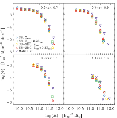
Figure 8: Dependence of the mass function on the details of the stellar mass estimates, considering five different cases. Specifically, the points correspond to different choices of the stellar population synthesis code, metallicity ($Z$), extinction law (SB+SMC or SB alone), or the addition of secondary bursts to the smooth star-formation histories. Four cases correspond to SED fitting using Hyperzmass, for which the values of the adopted parameters are given in the bottom-left of the first panel. For details about the parameters adopted for MAGPHYS (downward triangle), we refer to Sect. 2.3.

The other estimates, produced by Hyperzmass, are in quite good agreement with each other. The mass functions are slightly higher (on average by about $0.1$ dex) when obtained through SED fitting procedures that can choose between two values of metallicity. In fact, in this case, red galaxies can be fit with $0.2\,Z_{\odot}$ and older ages, consequently resulting in higher stellar mass values. The effect of the extinction law is instead marginal.

4 Comparison to previous work

In this section we compare the VIPERS GSMF with other mass functions derived from different galaxy surveys (Sect. 4.1) and various semi-analytical models (Sect. 4.2).

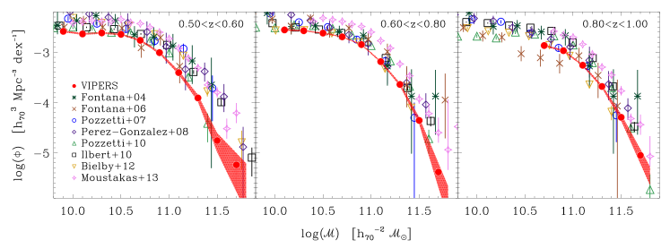
Figure 9: The VIPERS galaxy stellar mass functions from $z=0.5$ to $1$ (filled red circles, with a red shaded area accounting for the Poisson uncertainty). The $1/V_{\mathrm{max}}$ determinations of previous surveys are also shown by different symbols, along with their respective Poisson error bars. In the left-hand panel, whereas the VIPERS range is $0.5<z<0.6$, the other GSMFs are computed between $z=0.4$ and $0.6$, with the exception of Moustakas et al. (2013) for which is $0.5<z<0.65$, $0.65<z<0.8$, $0.8<z<1.0$; notice the very small error bars of the VIPERS data, despite the narrower redshift range. In the other two panels, the bins of VIPERS are the same as the other surveys; also at these higher redshifts the error bars of the VIPERS GSMF are small compared to them.

4.1 Comparison with other observational estimates

We compare here our estimate of the GSMF with results from other galaxy surveys. We correct GSMFs (if necessary) to be in the same cosmological model with $\Omega_{m}=0.3$, $\Omega_{\mathbf{\Lambda}}=0.7$, $h_{70}=1$, and Chabrier (2003) IMF. We also modify our binning in redshift to be similar to other work.

We chose eight surveys that adopt comparable $z$-bins, half of them based on photometric redshifts (Fontana et al., 2006; Pérez-González et al., 2008; Ilbert et al., 2010; Bielby et al., 2012) and half on spectroscopic redshifts (Fontana et al., 2004; Pozzetti et al., 2007, 2010; Moustakas et al., 2013). The spectroscopic redshift sample used by Moustakas et al. (2013) is obtained through a pioneering technique based on a low dispersion prism and slitmasks (Coil et al., 2011), which results in a precision of $\sigma_{z}\simeq 0.007(1+z)$ (for their high quality sample $Q\geqslant 3$, see Cool et al., 2013), i.e. comparable to the precision of the best photometric redshifts (Ilbert et al., 2013, who obtain $\sigma_{z}\simeq 0.008(1+z)$ and a very low percentage of outliers).

The redshift ranges of the GSMFs shown in Fig. 9 are $0.4<z<0.6$, $0.6<z<0.8$, $0.8<z<1.0$, with the exception of PRIMUS (Moustakas et al., 2013), which is at $0.5<z<0.65$, $0.65<z<0.8$, $0.8<z<1.0$, and the first bin of VIPERS (i.e., $0.5<z<0.6$). In the case of Bielby et al. (2012), who provide the GSMFs in four CFHTLS-Deep quadrants, we consider the results in the D3 field ($1\,440\,\mathrm{arcmin}^{2}$), which is located in a region of sky uncorrelated with the other surveys we selected. For the VIPERS GSMFs we plot error bars accounting only for $\sigma_{\mathrm{Poiss}}$, i.e. without adding the uncertainty due to sample variance, in order to be consistent with most of the literature data, for which only Poisson errors are available.

Our results lie on the lower boundary of the range covered by other GSMFs, and are in reasonably good agreement with most of them. At $0.8<z<1.0$, the difference with Ilbert et al. (2010, COSMOS survey over $2\,\mathrm{deg}^{2}$) and Pozzetti et al. (2010, zCOSMOS, $1.4\,\mathrm{deg}^{2}$) is noteworthy: the likely reason is the presence of a large structure detected in the COSMOS/zCOSMOS field (Kovač et al., 2010), demonstrating the importance of the cosmic variance in this kind of comparison.

Some discrepancy (nearly by a factor of two) is also evident with the estimates by Moustakas et al. (2013). The explanation could be partly related to the statistical weighing, in particular for the faintest objects, because the lower the sampling rate estimates, the greater the uncertainty in such a correction. At magnitudes $i\simeq 22.5$, the SSR of PRIMUS is approximately $45$%, dropping below $20$% at the limit of the survey (Cool et al., 2013). Instead, in VIPERS the SSR is $\sim 75$% down to our magnitude limit $i=22.5$ and to $z\simeq 1$, making the statistical weight corrections smaller and more robust. In addition to this, it should be noticed that although several overdensities have been observed in PRIMUS, cosmic variance seems unable to fully justify the difference between the GSMFs of the two surveys: the number of independent fields (PRIMUS consists of five fields with a total of $5.5\,\mathrm{deg}^{2}$) should reduce this problem, at least to some degree. The disagreement could also be partially ascribed to the different ways stellar masses are estimated: Moustakas et al. derived their reference SEDs according to the SSP model of Conroy & Gunn (2010), which results in stellar mass estimates systematically higher than those obtained by assuming BC03 (see Moustakas et al., 2013, Fig. 19).

Regarding the choices of SEDs, it is worth noticing that Pérez-González et al. (2008) also used a template library different from ours, which they derived from the PEGASE stellar population synthesis model (Fioc & Rocca-Volmerange, 1997), bounding the parameter space by means of a training set of $\sim 2000$ galaxies with spectroscopic $z$ and wide photometric baseline. The other surveys quoted in Fig. 9 (Fontana et al., 2004, 2006; Pozzetti et al., 2007, 2010; Ilbert et al., 2010; Bielby et al., 2012) adopt BC03.

VIPERS data provide tight constraints on the high-mass end of the GSMF. Previous surveys, such as K20, MUSIC, and VVDS-Deep (i.e. Fontana et al., 2004, 2006; Pozzetti et al., 2007), were unable to probe this portion of the GSMF ($\log(\mathcal{M}/\mathcal{M}_{\odot})\gtrsim 11.5$) because of their relatively small area (about $52$, $150$, and $1\,750\,\mathrm{arcmin}^{2}$ respectively). Instead, GSMFs derived from photometric redshift surveys are characterised by a Poisson noise that is in general comparable to the level in VIPERS (Pérez-González et al., 2008; Ilbert et al., 2010), but they can be affected by failures on photometric redshift estimates: even a small fraction of catastrophic redshift measurements can be relevant at high masses (Marchesini et al., 2009, 2010). Moreover, the sky area generally covered by high-$z$ photometric surveys is not large enough for cosmic variance to be negligible.

We postpone a detailed analysis of the evolution of the GSMF down to the local Universe to future work: differences in the details of the available estimates from 2dFGRS, SDSS, and GAMA (see Cole et al., 2001; Bell et al., 2003; Panter et al., 2004; Baldry et al., 2008; Li & White, 2009; Baldry et al., 2012) prevent a robust comparison with our data. Only computing stellar masses and mass functions in a self-consistent way can provide constraints on the evolution of the GSMF down to $z=0$ (e.g. Moustakas et al., 2013).

4.2 Testing models

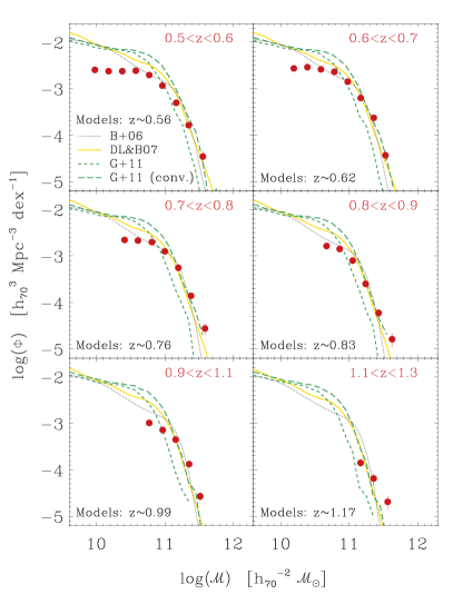
Figure 10: Comparison of the VIPERS mass function (red points, as in Fig. 5) with the semi-analytical models of Bower et al. (2006), De Lucia & Blaizot (2007), and Guo et al. (2011) (grey dotted, yellow solid, green short-dashed lines), whose GSMFs have been derived directly from the tables available in the Millennium database (Lemson & Virgo Consortium, 2006). The Guo et al. (2011) stellar masses have also been convolved with a Gaussian of dispersion $0.15$ dex, to reproduce observational uncertainty on stellar mass determinations; the resulting GSMFs are represented with green long-dashed lines.

Besides the comparison with other surveys, it is important to check the agreement of our results with simulations. In this paper we limit ourselves to a preliminary analysis. Nevertheless, this first test provides intriguing results.

The four semi-analytical models (SAMs) we consider here rely on the halo-merger trees of the Millennium Simulation (MS Springel et al., 2005) and the Millennium-II Simulation (MSII Boylan-Kolchin et al., 2009); namely, three of them (Bower et al., 2006; De Lucia & Blaizot, 2007; Mutch et al., 2013) use the MS (comoving box size $L=714\,\mathrm{Mpc}\,h_{70}^{-1}$, particle mass $=1.23\times 10^{9}\,\mathcal{M}_{\odot}\,h_{70}^{-1}$), while the last one (Guo et al., 2011) is based on both MSI and MSII ($L=143\,\mathrm{Mpc}\,h_{70}^{-1}$, particle mass $=9.83\times 10^{6}\,\mathcal{M}_{\odot}\,h_{70}^{-1}$). The tight constraints posed by VIPERS can be very useful when studying whether these models adequately reproduce the real universe.

In Fig. 10, we show the mass functions derived from the models of Bower et al. (2006), De Lucia & Blaizot (2007), and Guo et al. (2011), together with the VIPERS results. All the model GSMFs are computed from snapshots at the same redshifts. The narrow redshift binning we can set in VIPERS ($\Delta z=0.1$) allows us to compare simulated galaxies to observed ones at cosmic times that are very close to the snapshot considered. In the case of De Lucia & Blaizot model, we also derived the stellar mass functions from the VIPERS-like light cones introduced in Sect. 3.3, but we do not show them in Fig. 10 since they lead to results that are indistinguishable from those obtained from snapshots. For all three SAMs, we find that the low-mass end of the GSMF is over-estimated. Such a discrepancy, already observed in other work (Somerville et al., 2008; Cirasuolo et al., 2010), is mainly due to an over-predicted fraction of passive galaxies on those mass scales. This can be caused by an under-efficient supernova feedback and/or some issue as to how the star formation efficiency is parametrised at high redshifts (Fontanot et al., 2009; Guo et al., 2011). Rescaling the simulations to an up-to-date value of $\sigma_{8}$ (in MS it is equal to $0.9$), with the consequence of reducing the small-scale clustering of dark-matter haloes, alleviates the tension only in part (Wang et al., 2008; Guo et al., 2013).

At a first glance, De Lucia & Blaizot (2007) and Bower et al. (2006) seem to agree with the observed GSMFs at $\log(\mathcal{M/M_{\odot}})\gtrsim 11.0$, while the Guo et al. (2011) mass function lies systematically below by $\simeq 0.4$ dex. However, it should be emphasised that in Fig. 10 we plotted the GSMFs from SAMs without taking the observational uncertainties on stellar mass into account. We verified that adding this kind of error would increase the density of massive objects in the exponential tail of the mass function, and therefore the De Lucia & Blaizot (2007) and Bower et al. (2006) results should be considered at variance with observations also at $\log(\mathcal{M}/\mathcal{M}_{\odot})\geqslant 11$.

The effect of introducing observational uncertainties is shown in Fig. 10 only for the Guo et al. (2011) model, which foresees a lower density of objects in the massive end with respect to the other two models. We recomputed the Guo et al. GSMFs after convolving stellar masses with a Gaussian of dispersion $0.15$ dex. The predictions of Guo et al. (2011) are then in fair agreement with VIPERS. With respect to De Lucia & Blaizot (2007), the main distinguishing features of Guo et al. (2011) model are the high efficiency of supernova feedback and a lower rate of gas recycling at low mass. The transition from central to satellite status in the Guo et al. prescription also differs, resulting in a larger number of satellite galaxies than in De Lucia & Blaizot model.

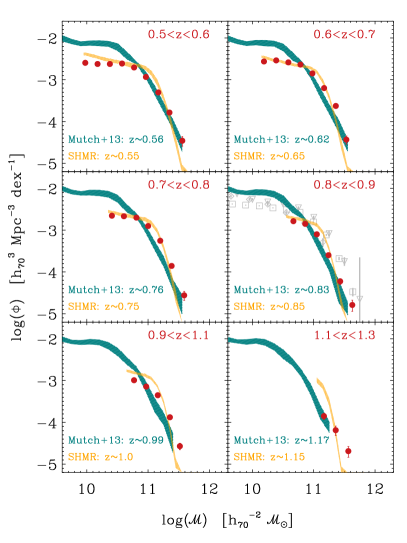
Figure 11: Comparison of the VIPERS mass function (red points) with the semi-analytical model of Mutch et al. (2013) (green shaded area at $95$% confidence limits). In several redshift bins Mutch et al. GSMF does not reach masses as high as VIPERS because the volume of the simulation (with a comoving box size $L=89.3\,\mathrm{Mpc}\,h_{70}^{-1}$) is smaller. In the right-hand middle panel ($0.8<z<0.9$), a grey dashed line represents the mass function that Mutch et al. obtain by combining observational data from three different surveys (Pozzetti et al., 2007; Drory et al., 2009; Ilbert et al., 2010, grey triangles,diamonds, and squares, respectively). In addition, the yellow shaded regions represent the dispersion of the mass functions derived from the $57$ SHMR mocks (see Sect. 3.3), in the same redshift bins as the VIPERS ones.

It should be emphasised that only Guo et al. (2011) choose most of the parameters in order to fit the observed local mass function, whereas Bower et al. (2006) and De Lucia & Blaizot (2007) use the local luminosity function to adjust their recipes. In recent studies, the parameters of these models have been tuned [again] by means of a different approach, based on Bayesian inference (Henriques et al., 2009; Bower et al., 2010). From this perspective, a particular kind of calibration has been proposed by Mutch et al. (2013), who modify the input parameters in the SAM of Croton et al. (2006) to match observations at $z=0$ and $z\simeq 0.8$ simultaneously.

The results obtained by Mutch et al. (2013) are compared to the VIPERS mass functions in Fig. 11. The plot shows reasonable agreement beyond $\mathcal{M}\simeq 10^{11}\,\mathcal{M}_{\odot}$, not only at the redshift of calibration ($z\simeq 0.83$) but also in the other bins. The authors do not convolve their mass functions with a Gaussian uncertainty on stellar masses, because at least part of the uncertainties this procedure accounts for should already be included in the observational constraints they use. The Mutch et al. (2013) model is calibrated at $z=0.83$ by using the results of Pozzetti et al. (2007), Drory et al. (2009), and Ilbert et al. (2010). Among these three GSMFs, only Pozzetti et al. (2007) is based on spectroscopic data (VVDS-Deep), which are unfortunately quite limited at high masses. The other two estimates (Drory et al., 2009; Ilbert et al., 2010) are derived from the COSMOS survey, which contains a significant over-density at $z\simeq 0.8$. The strategy adopted by Mutch et al. to combine such information may lead to overconfidence in the adopted constraints, especially in the highest mass range, where observations are most difficult. To reconcile SAM and observations at $\log(\mathcal{M}/\mathcal{M}_{\odot})>10.8$, Mutch et al. (2013) have assumed a star formation efficiency much higher than the one imposed by Croton et al. (2006), and consequently they were forced to parametrise supernova feedback efficiency with a range of values that is not completely supported by observations (Rupke et al., 2002; Martin, 2006). Intriguingly, we note that the authors would significantly relieve these tensions if they were to add VIPERS data to their analysis.

From a different perspective, the SHMR mocks we introduced in Sect. 3.3 are also calibrated at multiple redshifts. We decided to test their reliability by deriving their GSMFs (Fig. 11). The agreement is remarkable: VIPERS data confirm the validity of the stellar-to-halo mass relation of Moster et al. (2013) that was used to construct these mocks. This relation connects galaxies with their hosting dark matter halo by means of a redshift-dependent parametrisation that has been calibrated through the GSMFs of Pérez-González et al. (2008) and Santini et al. (2012) up to $z=4$. Because of the lack of tight constraints used by Moster et al. for the most massive galaxies (the data from Pérez-González et al., 2008 have lower statistics than ours), the SHMR mass functions diverge at high mass from our estimates.

5 Evolution of the mass function of the red and blue galaxy populations

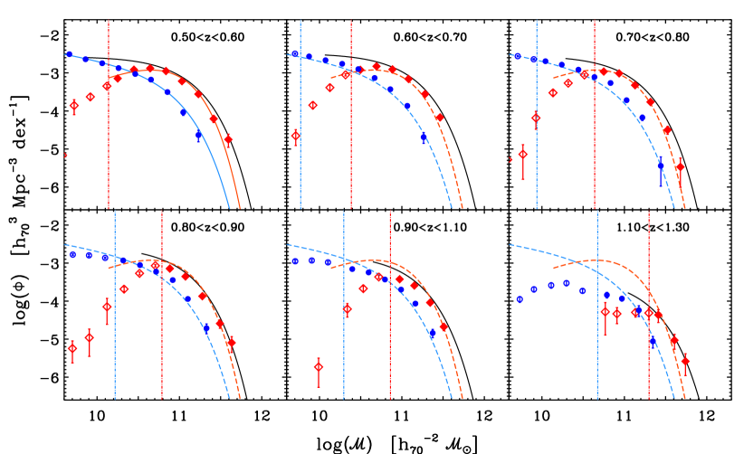
Figure 12: The galaxy stellar mass functions of the blue and red populations in VIPERS, derived using the $1/V_{\mathrm{max}}$. Symbols (circles and diamonds, respectively) are filled for data above the corresponding completeness limit $\mathcal{M}_{\mathrm{lim}}$ (vertical lines) and empty below. Error bars account for Poisson noise alone. The Schechter fit of the two populations in the bin $0.5<z<0.6$ (solid blue and red lines) is reported for reference as a dashed line in the other panels. The solid black line in each panel gives the Schechter best fit to the whole VIPERS sample in that redshift bin.

In order to distinguish the contribution of quiescent and actively star forming galaxies to the global evolution, we now split the sample according to the galaxy rest-frame $(U-V)$ colour (see Fritz et al., 2013 for extensive discussion).

5.1 Classification of galaxy types

The absolute magnitudes for galaxies in the VIPERS catalogue were computed from the same SED fitting procedure described in Sect. 2.3, applying a k- and colour-correction, derived from the best-fit SED, to the apparent magnitudes in the bands that more closely match the rest-frame emission in the $U$ and $V$ filters (see details in Fritz et al., 2013). In this way, $(U-V)$ rest-frame colours can be reliably computed within the redshift range of the survey, showing the classical bimodality and allowing us to separate red-sequence from blue-cloud galaxies (cf. Strateva et al., 2001; Hogg et al., 2002; Bell et al., 2004).

The valley between the two populations is found to be slightly evolving toward bluer colours at earlier epochs. Despite its simplicity, this photometric classification can be considered as a good proxy for selecting quiescent and star-forming galaxies. As discussed by Mignoli et al. (2009) using zCOSMOS data, $86$% ($93$%) of the galaxies selected as being photometrically red (blue) are also quiescent (star-forming) according to their spectra.

To verify and validate our selection method, we also derived galaxy photometric types by fitting our photometry with the empirical set of $62$ templates used in Ilbert et al. (2006), which was optimised to refine the match between photometric and spectroscopic redshifts in the VVDS. The same set was also used to classify galaxies in several other papers (e.g. Zucca et al., 2006, 2009; Pozzetti et al., 2010; Moresco et al., 2010). The classification of VIPERS galaxies resulting from this second method matches reasonably well with the $(U-V)$ colour selection. More than $70$% of the red galaxies are defined as early-type objects by the SED analysis, while more than $95$% of blue galaxies are classifed as late types. For red galaxies this worsens beyond $z=1.1$, where only $55$% of the red galaxies are classified as early types in terms of their SED. In the same redshift range, instead, $98$% of blue galaxies are classified as late-type objects.

5.2 Blue and red galaxy stellar mass functions

Using this classification, we are now in a position to quantify the contribution of red and blue galaxies to the GSMF and, in particular, to its high-mass end. The results are shown in Fig. 12. The mass functions for each class are estimated in bins of $0.2$ in $\log(\mathcal{M})$, using the same $1/V_{\mathrm{max}}$ method as described in Sect. 3.2. Fits with the usual Schechter function are provided, as described in the caption, to highlight evolution (or absence thereof) as a function of redshift.

The predominance of red objects among the massive galaxies is clearly visible in all redshift bins, with blue galaxies mainly contributing at lower masses ($\mathcal{M}<\mathcal{M}_{\star}$). Since the mass completeness limit $\mathcal{M}_{\rm lim}$ for the blue population extends to sufficiently low masses, we can perform the Schechter fit by leaving $\mathcal{M}_{\star}$, $\Phi_{\star}$, and $\alpha$ free. The slope of the low-mass end remains almost constant in redshift for the blue population, with $1.2<\alpha<1.3$, up to $z\simeq 0.9$, as seen in previous works (cf. Pozzetti et al., 2010). At redshift higher than this it can no longer be constrained. With respect to the red population, the high values of the mass completeness limit $\mathcal{M}_{\mathrm{lim}}$ (see Sect. 3.1) prevent us from studying the red sample in the same mass range; for instance, it is not possible to determine the evolution of $\alpha$ (Ilbert et al., 2010) or an upturn of the GSMF (cf. Drory et al., 2009) in a reliable way.

From these measurements we can determine the value of $\mathcal{M}_{\mathrm{cross}}$, where the blue and red GSMFs intersect, i.e. the dividing line between the ranges in which blue and red galaxies respectively dominate the mass function (Kauffmann et al., 2003b). The physical meaning of $\mathcal{M}_{\mathrm{cross}}$ has been questioned (Bell et al., 2007), but it is in general considered as a proxy to the transition mass of physical processes such the quenching of star formation, (responsible for the migration from the blue cloud to the red sequence), or the AGN activity (e.g. Kauffmann et al., 2003a). Moreover, its clear dependence on environment (Bolzonella et al., 2010) points to an interpretation of the galaxy transformation that is not only linked to secular processes.

We quantify the value of the transition mass in each redshift bin using the $1/V_{\mathrm{max}}$ measurements. The transition mass increases from $\log(\mathcal{M}_{\mathrm{cross}}/\mathcal{M}_{\odot})=10.4$ at $z\simeq 0.55$ to $\log(\mathcal{M}_{\mathrm{cross}}/\mathcal{M}_{\odot})=10.6$ at $z\simeq 0.75$, as shown in Fig. 13. This trend is very well fitted by a power law $\propto(1+z)^{3}$. Beyond $z=0.8$ our $\mathcal{M}_{\mathrm{cross}}$ estimates should be formally considered as upper limits, since they fall below the mass completeness limit of red galaxies, but at least up to $z=1.0$, they can be considered as a good approximation of the real values, given their proximity to the limit.

In Fig. 13 we also plot results from previous studies. In this respect, it is important to underline that the value of $\mathcal{M}_{\mathrm{cross}}$ provided by the various authors can differ significantly from each other, depending on the adopted classification. For instance, the results of the morphological classification used by Bundy et al. (2006) on the DEEP2 survey fall above the mass ranges considered in the plot. This could be related to part of the “red and dead” galaxies at such redshifts becoming ellipticals (in a morphological sense) at a later stage (Bundy et al., 2010). In fact, when we split the DEEP2 sample on the basis of the $(U-B)$ bimodality, the results are in agreement with our findings. Our estimates of $\mathcal{M}_{\mathrm{cross}}$ are fairly consistent (within $\pm 0.2\,\mathrm{dex}$ approximatively) with those of Vergani et al. (2008), Pozzetti et al. (2010), Moustakas et al. (2013). The estimates by Vergani et al. (2008), also shown in Fig. 13, rely on the identification of the D$4000$ break in the VVDS spectra and have a steeper redshift evolution, $\mathcal{M}_{\mathrm{cross}}\propto(1+z)^{4}$. Pozzetti et al. (2010) derived $\mathcal{M}_{\mathrm{cross}}$ from the GSMFs of the zCOSMOS (10k-bright) sample split using different criteria: a cut in specific SFR (i.e. sSFR $\equiv{\rm SFR}/\mathcal{M}\gtrless 10^{-1}\mathrm{Gyr}^{-1}$), morphology (spheroidal vs disc/irregular galaxies), and best-fit SEDs (same photometric types discussed in Sect. 5.1). Moustakas et al. (2013) define star-forming galaxies as lying in the so-called main sequence of the SFR (estimated from the SED fitting) versus $\mathcal{M}$ diagram (Noeske et al., 2007). They find a flatter evolution, with $\mathcal{M}_{\mathrm{cross}}\propto(1+z)^{1.5}$.

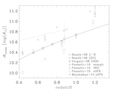
Figure 13: The values of the transition mass $\mathcal{M}_{\mathrm{cross}}$ as computed from Fig. 12, plotted as a function of redshift. The VIPERS measurements are given as black open circles, with a downward arrow when the transition mass is below the completeness mass of at least one of the two classes. The solid line is a fit with a $(1+z)^{3}$ power law to the VIPERS points between $z=0.5$ and $z=0.8$. These are compared to literature estimates in grey. Points from Pozzetti et al. (2010) are obtained using three different classifications: a separation according to specific SFR (diamonds), a best-fit SED classification (triangles), and a morphological classification (squares). The points of Bundy et al. (2006) are based on either the $(U-B)$ bimodality or [OII] emission (upper and lower half-circles respectively). The points by Vergani et al. (2008) (asterisks) are based on a spectral classification (D4000 break). The value from PRIMUS (Moustakas et al., 2013) at $z=0.9$ is reported as a cross, while the dashed line traces an evolution $\propto(1+z)^{1.5}$, as suggested in that paper; these authors classified active and quiescent galaxies with respect to their position in the SFR vs $\mathcal{M}$ diagram.

5.3 Evolution of the blue and red populations

To collect further evidence of star-formation quenching processes that cause the transition of galaxies from the so-called blue cloud to the red sequence (Faber et al., 2007), we measured the evolution of the galaxy number density of blue and red populations, namely $\rho_{N}^{\rm blue}(z)$ and $\rho_{N}^{\rm red}(z)$. These estimates are derived using the $1/V_{\mathrm{max}}$ method, taking both Poisson noise and cosmic variance into account. We also verified, however, that the results would essentially be the same if we had measured number densities by integrating the Schechter best-fitting functions. We explore four narrow bins of stellar mass to highlight the dependence of the quenching processes on this parameter. To improve statistics at high stellar masses, we choose wider redshift bins here: $0.5$–$0.7$, $0.7$–$0.9$, $0.9$–$1.1$, $1.1$–$1.3$.

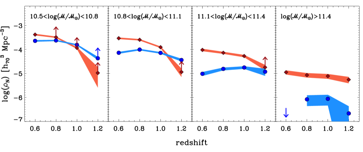
Figure 14: Evolution of the number density of the blue and red galaxy populations in VIPERS (filled circles and diamonds, respectively) with different stellar masses. Upward arrows represent lower limits when $\rho_{N}$ is estimated in a bin of mass affected by incompleteness, while a downward arrow represents the upper limit in case of zero detection (rightmost panel). The error corridors reflect the overall uncertainties, which include both Poisson noise and cosmic variance added in quadrature.

At intermediate masses ($10.8<\log(\mathcal{M}/\mathcal{M}_{\odot})<11.1$), the number density of red galaxies $\rho_{N}^{\rm red}$ increases by a factor of $\sim 2.5$ from $z\!=\!1$ to $z\!=\!0.6$, whereas at higher masses the variation is much smaller. Red galaxies with mass $11.1<\log(\mathcal{M}/\mathcal{M}_{\odot})<11.4$ evolve from a number density $\rho_{N}^{\rm red}=(5.3\pm 0.6)\times 10^{-5}\,\mathrm{Mpc}^{-3}\,h_{70}^{3}$ to $(9.5\pm 1.1)\times 10^{-5}\,\mathrm{Mpc}^{-3}\,h_{70}^{3}$ in the same redshift interval (about $80$% increase). The increase is even smaller ($45\%$) for galaxies with $\log(\mathcal{M/M}_{\odot})\geqslant 11.4$. With the VIPERS data we are able for the first time to provide significant evidence of this trend for such massive galaxies at these redshifts. This result is in line with the mass-assembly downsizing scenario highlighted in previous works (Cimatti et al., 2006; Pozzetti et al., 2010; Ilbert et al., 2010): barring systematic effects due to the uncertainty on $\mathcal{M}$, red galaxies with $\mathcal{M}>10^{11}\,\mathcal{M}_{\odot}$ build their stellar mass well before the less massive ones and do not experience any strong evolution between $z\simeq 1.2$ and $z\simeq 0.6$. At these redshifts, quenching mechanisms seem to be more efficient at low and intermediate masses, as also recently suggested by Moustakas et al. (2013). With respect to PRIMUS, the VIPERS survey extends this finding to higher masses ($\log(\mathcal{M/M}_{\odot})>11.4$) and redshifts (up to $\simeq 1.2$). The evidence of mass dependence of quenching agrees, for instance, with Peng et al. (2010), although other mechanisms could play a non-negligible role (e.g. galaxy mergers, Xu et al., 2012).

The co-moving number density of blue galaxies is instead found to be relatively stable between $z\simeq 1$ to $z\simeq 0.6$ for objects with mass $10.5\leqslant\log(\mathcal{M/M}_{\odot})<10.8$, with a $10\%$ variation. For higher mass blue galaxies, for which the sample is complete at all redshifts, the density $\rho_{N}^{\mathrm{blue}}$ of objects with mass $10.8\leqslant\log(\mathcal{M/M}_{\odot})<11.1$ indicates a mild increase between $z\simeq 1.2$ and $z=0.8$.

The most massive blue galaxies ($\log(\mathcal{M/M}_{\odot})\geqslant 11.4$) disappear at $z\lesssim 0.6$ (see the right panel in Fig. 14), suggesting that, at such high masses, star formation already turns off at earlier epochs (i.e. $z>1.3$). When the whole VIPERS sample is available, we will continue the analysis of the massive-end build-up with more robust statistics. Moreover, a step forward for a better comprehension of this picture will be the use of spectral features to determine reliable estimates of the SFR, and therefore to better separate passive and active galaxies.

6 Conclusions

We measured the GSMF between $z=0.5$ and $z=1.3$ using the first data release of VIPERS. The forthcoming VIPERS Public Data Release 1 (PDR-1) will contain the catalogue of the $53\,608$ spectroscopic galaxy redshifts used in the present analysis. The galaxy stellar masses were estimated through the SED fitting technique, relying on a large photometric baseline and, in particular, on a nearly full coverage of our fields with near-infrared data. We performed several tests to verify that the systematics intrinsic to the method of SED fitting (e.g. the parametrisation of the SFH) do not introduce any significant bias into our analysis. The large volume probed by VIPERS results in extremely high statistics, dramatically reducing the uncertainties due to Poisson noise ($\sigma_{\mathrm{Poiss}}$) and sample variance ($\sigma_{\mathrm{cv}}$). We estimated the latter by using $57$ galaxy mock catalogues based on the MultiDark simulation (Prada et al., 2012) and the stellar-to-halo mass relation of Moster et al. (2013). These mocks closely reproduce the characteristics of the VIPERS survey.

We empirically determined a completeness threshold $\mathcal{M}_{\mathrm{lim}}$ above which the mass function can be considered complete. This limiting mass evolves as a function of $z$, ranging from $\log(\mathcal{M/M}_{\odot})=9.8$ to $11$ in the redshift interval $0.5$–$1.1$. We focussed our analysis on the high-mass end of the GSMF, where VIPERS detects a particularly high number of rare massive galaxies. The main results we obtain follow.

• VIPERS data tightly constrain the exponential tail of the Schechter function, which does not show significant evolution at high masses below $z=1.1$. The same result is provided by analysis of the co-moving number density $\rho_{N}$, calculated in different bins of stellar mass. At $z\simeq 1.2$ most of the massive galaxies with $\log(\mathcal{M/M}_{\odot})\geqslant 11.4$ are already in place, whereas below $\log(\mathcal{M/M}_{\odot})=11.4,$ the galaxy number density increases by a factor of $\sim 3.5$ from $z\simeq 1.2$ to $z\simeq 0.6$.

• We compared our observed GSMFs with those derived from semi-analytical models (De Lucia & Blaizot, 2007; Bower et al., 2006; Guo et al., 2011). While the discrepancy at low masses between models and observations is well established and has been exhaustively discussed in literature, predictions at the high-mass end of the GSMF have not yet been verified with sufficient precision. We show that the high accuracy of the VIPERS mass functions makes them suitable for this kind of test, although further improvement to reduce stellar mass uncertainties would be beneficial. From a first analysis, the VIPERS data appear to be consistent with the Guo et al. (2011) model at $\log(\mathcal{M/M_{\odot}})\geqslant 11$, once the uncertainties in the stellar mass estimates are taken into account. A more detailed analysis will be the subject of a future work. We suggest that VIPERS GSMFs can be effectively used to constrain models at multiple redshifts simultaneously, in small steps of $\Delta z$. This could shed light on the time scale of the physical mechanisms that determine the evolution at higher masses (for instance, the AGN-feedback efficiency).

• We divided the VIPERS sample by means of a colour criterion based on the $(U-V)$ bimodality (Fritz et al., 2013) and estimated the blue and red GSMF in the same range, $0.5<z<1.3$. We find that the transition mass above which the GSMF is dominated by red galaxies is about $\log(\mathcal{M_{\mathrm{cross}}/M}_{\odot})\simeq 10.4$ at $z\simeq 0.55$ and evolves proportional to $(1+z)^{3}$.

• The number density of the red sample shows an evolution that depends on stellar mass, being steeper at lower masses. At high stellar masses, the quenching of active galaxies has not been thoroughly studied because of their rareness. We obtained a first impressive result with VIPERS, by detecting at $z\simeq 1$ a significant number of very massive active galaxies with $\log(\mathcal{M/M}_{\odot})\geqslant 11.4$, which have all migrated onto the red sequence by $z=0.6$, i.e. in about $2$ Gyrs.

The first data release of VIPERS has allowed us to study the evolution of the galaxy stellar mass function over an unprecedented volume at redshifts $z=0.5-1.3$. We emphasise the constraining power of this dataset, particularly for the abundance of the most massive galaxies, both quiescent and star-forming. In forthcoming studies we will make full use of the growing sample and of the measurement of spectral features, in order to investigate the cosmic star formation history and compare galaxy formation models at high redshift.