Entire solutions with exponential growth for an elliptic system modeling phase-separation

Abstract.

We prove the existence of entire solutions with exponential growth for the semilinear elliptic system

$$\begin{cases}-\Delta u=-uv^{2}&\text{in $\mathbb{R}^{N}$}\\ -\Delta v=-u^{2}v&\text{in $\mathbb{R}^{N}$}\\ u,v>0,\end{cases}$$

for every $N\geq 2$. Our construction is based on an approximation procedure, whose convergence is ensured by suitable Almgren-type monotonicity formulae. The construction of some solutions is extended to systems with $k$ components, for every $k>2$.

Nicola Soave

Università degli Studi di Milano Bicocca - Dipartimento di Matematica e Applicazioni

Via Roberto Cozzi 53, 20125 Milano, Italy

email: n.soave@campus.unimib.it

Alessandro Zilio

Politecnico di Milano - Dipartimento di Matematica “Francesco Brioschi”

Piazza Leonardo da Vinci 32, 20133 Milano, Italy

email: alessandro.zilio@mail.polimi.it

Keywords: elliptic system, phase-separation, Almgren monotonicity formulae, entire solutions, exponential growth.

1. Introduction and main results

In this paper we investigate the existence of entire solutions with exponential growth for the semilinear elliptic system

(1.1) $$\begin{cases}-\Delta u=-uv^{2}\\ -\Delta v=-u^{2}v\\ u,v>0,\end{cases}$$

in $\mathbb{R}^{2}$ (thus in $\mathbb{R}^{N}$ for every $N\geq 2$). System (1.1), which appears in the study of phase-separation phenomena for Bose-Einstein condensates with multiple states, has been intensively studied in the last years; we refer in particular to [1, 3, 4, 5, 9, 10], where physical motivations are discussed and a precise description of the phase-separation is derived, and to [1, 2] where existence and qualitative properties of entire solutions are central topics. In [9], it is proved that if $(u,v)$ is an entire solution to (1.1) and is globally $\alpha$-Hölder continuous for some $\alpha\in(0,1)$, then one between $u$ and $v$ is constant while the other is identically $0$. On the other hand, in [1] the authors show that there exists a nontrivial solution for the system of ODEs

$$\begin{cases}-u^{\prime\prime}=-uv^{2}&\text{in $\mathbb{R}$}\\ -v^{\prime\prime}=-u^{2}v&\text{in $\mathbb{R}$}\\ u,v>0\end{cases}$$

which is reflectionally symmetric with respect to a point of $\mathbb{R}$, in the sense that there exists $t_{0}\in\mathbb{R}$ such that $u(t_{0}+t)=v(t_{0}-t)$ for every $t\in\mathbb{R}$, and has linear growth: there exists $C>0$ such that

$$u(t)+v(t)\leq C(1+|t|)\qquad\forall t\in\mathbb{R}.$$

The paper [2] completes the study of the $1$-dimensional problem with the proof of the uniqueness of the positive $1$-dimensional profile, up to translations and scalings. Always in [2], the authors construct entire solutions to (1.1) with algebraic growth for any integer rate of growth greater then $1$; here and in the rest of the paper we say that $(u,v)$ has algebraic growth if there exist $p\geq 1$ and $C>0$ such that

$$u(x)+v(x)\leq C(1+|x|^{p})\qquad\forall x\in\mathbb{R}^{N}.$$

The solutions constructed in [2] are not $1$-dimensional, and are modeled on (we will be more precise later, see Remark 1.2) the homogeneous harmonic polynomials $\Re(z^{d})$, for every $d\geq 2$. There is a deep relationship between entire solutions to (1.1) and harmonic functions; this relationship has been established in [5, 9]. For instance, in case $(u,v)$ has algebraic growth, it is possible to show that up to a subsequence, the blow-down family, defined by

$$\left(u_{R}(x),v_{R}(x)\right)=\frac{R^{N-1}}{\int_{\partial B_{R}(0)}u^{2}+v^{2}}\left(u(Rx),v(Rx)\right),$$

is uniformly convergent in every compact subset of $\mathbb{R}^{N}$, as $R\to+\infty$, to a limiting profile $(\Psi^{+},\Psi^{-})$, where $\Psi$ is a homogeneous harmonic polynomial (see Theorem 1.4 in [2]).

To conclude this bibliographic introduction, we have to mention that major efforts have been done recently in order to prove classification results and in particular the $1$-dimensional symmetry of solutions to (1.1). This is motivated by the relationship between (1.1) and the Allen-Cahn equation, which has been established in [1], and led the authors to formulate a De Giorgi’s-type and a Gibbons’-type conjecture for solutions to (1.1); for results in this direction, we refer to [1, 2, 6, 7, 11].

Motivated by the quoted achievements, we wonder if the system (1.1) has solutions with super-algebraic growth. We can give a positive answer to this question proving the existence of solutions with exponential growth. In our construction we adapt the same line of reasoning introduced in the proof of Theorem 1.3 of [2]. Therein, the authors proved the existence of solutions to (1.1) with the same symmetry of the function $\Re(z^{d})$ in any bounded ball $B_{R}(0)\subset\mathbb{R}^{2}$, with boundary conditions $u=(\Re(z^{d}))^{+}$, $v=(\Re(z^{d}))^{-}$ on $\partial B_{R}(0)$. By means of suitable monotonicity formulae, they could pass to the limit for $R\to+\infty$ obtaining convergence (up to a subsequence) for the previous family to a nontrivial entire solution. In this sense, their solutions are modeled on the harmonic functions $\Re(z^{d})$.

Here, having in mind the construction of solutions with exponential growth, and recalling the relationship between entire solution of our system and harmonic functions, we start by considering

$$\Phi(x,y):=\cosh x\sin y.$$

The first of our main results is the following.

Theorem 1.1.

There exists an entire solution $(u,v)\in(\mathcal{C}^{\infty}(\mathbb{R}^{2}))^{2}$ to system (1.1) such that

• $u(x,y+2\pi)=u(x,y)$ and $v(x,y+2\pi)=v(x,y)$,

• $u(-x,y)=u(x,y)$ and $v(-x,y)=v(x,y)$,

• the symmetries

  $$v(x,y)=u(x,y-\pi)\quad \quad u(x,\pi-y)=v(x,\pi+y)$$

  $$u\left(x,\frac{\pi}{2}+y\right)=u\left(x,\frac{\pi}{2}-y\right)\quad \quad v\left(x,\frac{3}{2}\pi+y\right)=v\left(x,\frac{3}{2}\pi-y\right)$$

  hold,

• $u-v>0$ in $\{\Phi>0\}$ and $v-u>0$ in $\{\Phi<0\}$,

• $u>\Phi^{+}$ and $v>\Phi^{-}$ in $\mathbb{R}^{2}$,

• the function (Almgren quotient)

  $$r\mapsto\frac{\int_{(0,r)\times(0,2\pi)}|\nabla u|^{2}+|\nabla v|^{2}+2u^{2}v^{2}}{\int_{\{r\}\times[0,2\pi]}u^{2}+v^{2}}$$

  is well-defined for every $r>0$, is nondecreasing, and

  $$\lim_{r\to+\infty}\frac{\int_{(0,r)\times(0,2\pi)}|\nabla u|^{2}+|\nabla v|^{2}+2u^{2}v^{2}}{\int_{\{r\}\times[0,2\pi]}u^{2}+v^{2}}=1,$$

• there exists the limit

  $$\lim_{r\to+\infty}\frac{\int_{\{r\}\times[0,2\pi]}u^{2}+v^{2}}{e^{2r}}=:\alpha\in(0,+\infty).$$

Remark 1.2.

This solution is modeled on the harmonic function $\Phi$, in the sense that it inherits the symmetries of $(\Phi^{+},\Phi^{-})$ and has the same rate of growth of $\Phi$.

Remark 1.3.

Point 7) of the Theorem gives a lower and a upper bound to the rate of growth of the quadratic mean of $(u,v)$ on $\{r\}\times[0,2\pi]$ when $r$ varies:

$$\left(\int_{\{r\}\times[0,2\pi]}u^{2}+v^{2}\right)^{\frac{1}{2}}=O(e^{r})\qquad\text{as $r\to+\infty$}.$$

The domain of integration takes into account the periodicity of $(u,v)$. The quadratic mean of $(u,v)$ on $\{r\}\times[0,2\pi]$ has exponential growth, and the rate of growth is the same of the function $e^{r}$, which in turns has the same rate of growth of $\Phi$. Note that the coefficient $1$ in the exponent of $e^{r}$ coincides with the limit as $r\to+\infty$ of the Almgren quotient defined in point 6).

Remark 1.4.

With a scaling argument, it is not difficult to prove the existence of entire solutions with exponential growth of order $\lambda$ for every $\lambda>0$ (in the previous sense). To see this, let

$$\left(u_{\lambda}(x,y),v_{\lambda}(x,y)\right)=\left(\lambda u(\lambda x,\lambda y),\lambda v(\lambda x,\lambda y\right).$$

It is straightforward to check that $(u_{\lambda},v_{\lambda})$ is still a solution to (1.1) in the plane, is $\frac{2\pi}{\lambda}$-periodic in $y$ and is such that

$$u_{\lambda}(x,y)\geq\lambda\left(\cosh(\lambda x)\sin(\lambda y)\right)^{+}\quad\text{and}\quad v_{\lambda}(x,y)\geq\lambda\left(\cosh(\lambda x)\sin(\lambda y)\right)^{-}.$$

Moreover,

(1.2) $$\lim_{r\to+\infty}\frac{\int_{(0,r)\times\left(0,\frac{2\pi}{\lambda}\right)}|\nabla u_{\lambda}|^{2}+|\nabla v_{\lambda}|^{2}+2u_{\lambda}^{2}v_{\lambda}^{2}}{\int_{\{r\}\times\left[0,\frac{2\pi}{\lambda}\right]}u_{\lambda}^{2}+v_{\lambda}^{2}}=\lambda,$$

and

$$\lim_{r\to+\infty}\frac{\int_{\{r\}\times\left[0,\frac{2\pi}{\lambda}\right]}u_{\lambda}^{2}+v_{\lambda}^{2}}{e^{2\lambda r}}=\lambda\alpha.$$

One can consider the solution $(u_{\lambda},v_{\lambda})$ as related to the harmonic function $\cosh(\lambda x)\sin(\lambda y)$. This reveals that there exists a correspondence

$$\{(u_{\lambda},v_{\lambda}):\lambda>0\}\leftrightarrow\{\sin(\lambda x)\cosh(\lambda y):\lambda>0\}.$$

Due to the invariance under translations and rotations of problem (1.1), the family $\{(u_{\lambda},v_{\lambda}):\lambda>0\}$ can equivalently be related with the families of harmonic functions $\{\cosh(\lambda x)\left[C_{1}\cos(\lambda y)+C_{2}\sin(\lambda y)\right]\}$ or $\{\left[C_{3}\cos(\lambda x)+C_{4}\sin(\lambda x)\right]\cosh(\lambda y):\lambda>0\}$, where $C_{1},C_{2},C_{3},C_{4}\in\mathbb{R}$.

As observed in Remark 1.3, the limit of the Almgren quotient in (1.2) describes the rate of the growth of the quadratic mean of $(u_{\lambda},v_{\lambda})$ computed on an interval of periodicity in the $y$ variable. The previous computation reveals that for every $\lambda>0$ we can construct a solution having rate of growth equal to $\lambda$. This marks a relevant difference between entire solutions with polynomial growth and entire solutions with exponential growth: while in the former case the admissible rates of growth are quantized (Theorem 1.4 of [2]), in the latter one we can prescribe any positive real value as rate of growth.

Remark 1.4 reveals that, starting from the solution found in Theorem 1.1, we can build infinitely-many entire solutions with different exponential growth. However, noting that system 1.1 is invariant under rotations, translations and scalings, intuitively speaking they are all the same solution. We wonder if there exists an entire solution of (1.1) having exponential growth which cannot be obtained by that found in Theorem 1.1 through a rotation, a translation or a scaling; the answer is affirmative. We denote

$$\Gamma(x,y):=e^{x}\sin y.$$

Theorem 1.5.

There exists an entire solution $(u,v)\in(\mathcal{C}^{\infty}(\mathbb{R}^{2}))^{2}$ to system (1.1) which enjoys points 1), 3), 4) of Theorem 1.1; moreover

• for every $r\in\mathbb{R}$

  (1.3) $$\int_{(-\infty,r)\times(0,2\pi)}|\nabla u|^{2}+|\nabla v|^{2}+u^{2}v^{2}<+\infty,$$

• $u>\Gamma^{+}$ and $v>\Gamma^{-}$ in $\mathbb{R}^{2}$,

• the function (Almgren quotient)

  $$r\mapsto\frac{\int_{(-\infty,r)\times(0,2\pi)}|\nabla u|^{2}+|\nabla v|^{2}+2u^{2}v^{2}}{\int_{\{r\}\times(0,2\pi)}u^{2}+v^{2}}$$

  is well-defined for every $r>0$, is nondecreasing, and

  $$\lim_{r\to+\infty}\frac{\int_{(-\infty,r)\times(0,2\pi)}|\nabla u|^{2}+|\nabla v|^{2}+2u^{2}v^{2}}{\int_{\{r\}\times(0,2\pi)}u^{2}+v^{2}}=1,$$

• there exist the limits

  $$\lim_{r\to+\infty}\frac{\int_{\{r\}\times[0,2\pi]}u^{2}+v^{2}}{e^{2r}}=:\beta\in(0,+\infty)\quad\text{and}\quad\lim_{r\to-\infty}\int_{\{r\}\times[0,2\pi]}u^{2}+v^{2}=0.$$

Remark 1.6.

This solution is modeled on the harmonic function $\Gamma$. As explained in Remark 1.3, it is possible to obtain a family of entire solutions which is in correspondence with a family of harmonic functions.

Remark 1.7.

Note that the Almgren quotients that we defined in Theorem 1.1 and 1.5 are different. They are both different to the Almgren quotient which has been defined in [2].

We can partially generalize our existence result to the case of systems with many components. To be precise, given an integer $k$, we will construct a solution $(u_{1},\dots,u_{k})$ of

(1.4) $$\begin{cases}-\Delta u_{i}=-u_{i}\sum_{j\neq i}u_{j}^{2}\\ u_{i}>0,\end{cases}i=1,\ldots,k,$$

in the whole plane $\mathbb{R}^{2}$ having the same growth and the same symmetries of $\Gamma$. Here and in the paper we consider the indexes $\mod k$.

Theorem 1.8.

There exists an entire solution $(u_{1},\dots,u_{k})\in(\mathcal{C}^{\infty}(\mathbb{R}^{2}))^{k}$ to system (1.4) such that, for every $i=1,\ldots,k$,

• $u_{i}(x,y+k\pi)=u_{i}(x,y)$,

• the symmetries

  $$u_{i+1}(x,y)=u_{i}\left(x,y-\pi\right)\quad\quad u_{1}\left(x,\frac{\pi}{2}+y\right)=u_{1}\left(x,\frac{\pi}{2}-y\right)$$

  hold,

• for every $r\in\mathbb{R}$

  $$\int_{(-\infty,r)\times(0,k\pi)}\sum_{i=1}^{k}|\nabla u_{i}|^{2}+\sum_{1\leq i<j\leq k}u_{i}^{2}u_{j}^{2}<+\infty;$$

• the function (Almgren quotient)

  $$r\mapsto\frac{\int_{(-\infty,r)\times(0,k\pi)}\sum_{i=1}^{k}|\nabla u_{i}|^{2}+2\sum_{1\leq i<j\leq k}u_{i}^{2}u_{j}^{2}}{\int_{\{r\}\times[0,k\pi]}\sum_{i=1}^{k}u_{i}^{2}}$$

  is well-defined for every $r>0$, is nondecreasing, and

  $$\lim_{r\to+\infty}\frac{\int_{(-\infty,r)\times(0,k\pi)}\sum_{i=1}^{k}|\nabla u_{i}|^{2}+2\sum_{1\leq i<j\leq k}u_{i}^{2}u_{j}^{2}}{\int_{\{r\}\times[0,k\pi]}\sum_{i=1}^{k}u_{i}^{2}}=1.$$

• there exist the limits

  $$\lim_{r\to+\infty}\int_{\{r\}\times[0,k\pi]}\sum_{i=1}^{k}u_{i}^{2}=:\gamma\in(0,+\infty)\quad\text{and}\quad\lim_{r\to-\infty}\int_{\{r\}\times[0,k\pi]}\sum_{i=1}^{k}u_{i}^{2}=0.$$

This solution is modeled on $\Gamma$.

Our last main result is the counterpart of Theorem 1.4 of [2] in our setting. This can be quite surprising because, as we already observed, we cannot expect a quantization of the admissible rates of growth dealing with solutions with exponential growth, see Remark 1.4. Nevertheless, if we consider solutions which are periodic in one component, prescribing a period such a quantization can be recovered.

Theorem 1.9.

Let $(u,v)$ be a nontrivial solution of (1.1) in $\mathbb{R}^{2}$ which is $2\pi$-periodic in $y$, and such that one of the following situation occurs:

• there holds

  $$\lim_{r\to-\infty}\int_{\{r\}\times[0,2\pi]}u^{2}+v^{2}=0,$$

  and

  $$d:=\lim_{r\to+\infty}\frac{\int_{(-\infty,r)\times(0,2\pi)}|\nabla u|^{2}+|\nabla v|^{2}+u^{2}v^{2}}{\int_{\{r\}\times[0,2\pi]}u^{2}+v^{2}}<+\infty.$$

• $\partial_{x}u=0=\partial_{x}v$ on $\{a\}\times[0,2\pi]$ for some $a\in\mathbb{R}$, and

  $$d:=\lim_{r\to+\infty}\frac{\int_{(a,r)\times(0,2\pi)}|\nabla u|^{2}+|\nabla v|^{2}+u^{2}v^{2}}{\int_{\{r\}\times[0,2\pi]}u^{2}+v^{2}}<+\infty.$$

Then $d$ is a positive integer,

$$\left(\int_{\{r\}\times[0,2\pi]}u^{2}+v^{2}\right)^{\frac{1}{2}}=O(e^{dr})\qquad\text{as $r\to+\infty$},$$

and the sequence

$$(u_{R}(x,y),v_{R}(x,y)):=\frac{1}{\sqrt{\int_{\{r\}\times[0,2\pi]}u^{2}+v^{2}}}\left(u(x+R,y),v(x+R,y)\right)$$

converges in $\mathcal{C}^{0}_{\mathrm{loc}}(\mathbb{R}^{2})$ and in $H^{1}_{\mathrm{loc}}(\mathbb{R}^{2})$ to $(\Psi^{+},\Psi^{-})$, where $\Psi(x,y)=e^{dx}\left(C_{1}\cos(dy)+C_{2}\sin(dy)\right)$ for some $C_{1},C_{2}\in\mathbb{R}$.

Notation.

We will deal with functions defined in domains of type $(a,b)\times\mathbb{R}$, where $a<b$ are extended real numbers ($a=-\infty$ and $b=+\infty$ are admissible). We will often assume that $(u_{1},\dots,u_{k})$ is $k\pi$-periodic in $y$; therefore, we can think to $(u_{1},\dots,u_{k})$ as defined on the cylinder

$$C_{(a,b)}:=(a,b)\times\mathbb{S}_{k}\quad\text{where}\quad\mathbb{S}_{k}=\mathbb{R}/(k\pi\mathbb{Z}).$$

We will also denote $\Sigma_{r}:=\{r\}\times\mathbb{S}_{k}$. In case $b>0$, $a=-b$, we will simply write $C_{b}$ instead of $C_{(-b,b)}$ to simplify the notation.

Plan of the paper.

In section 2 we will prove some monotonicity formulae which will come useful in the rest of the paper. We can deal with two types of solutions: solutions satisfying a homogeneous Neumann condition defined in a cylinder $C_{(a,b)}$ with $a>-\infty$, or solutions defined in a semi-infinite cylinder of type $C_{(-\infty,b)}$ and decaying at $x\to-\infty$. For the sake of completeness and having in mind to use some monotonicity formulae in the proof of Theorem 1.8, we will always consider the case of systems with $k$ components.

The proof of Theorem 1.1 will be the object of section 3. It follows the same sketch of the proof of Theorem 1.3 in [2]: we start by showing that for any $R>0$ there exists a solution $(u_{R},v_{R})$ to (1.1) in the cylinder $C_{R}$, with Dirichlet boundary condition

$$u_{R}=\Phi^{+}\quad\text{and}\quad v_{R}=\Phi^{-}\quad\text{on $\{-R,R\}\times[0,2\pi]$},$$

and exhibiting the same symmetries of $(\Phi^{+},\Phi^{-})$. In order to obtain a solution defined in the whole $C_{\infty}$, we wish to prove the $\mathcal{C}_{loc}^{2}(C_{\infty})$ convergence of the family $\{(u_{R},v_{R}):R>1\}$, as $R\to+\infty$. To show that this convergence occurs, we will exploit the monotonicity formulae proved in subsection 2.1. With respect to Theorem 1.3 of [2], major difficulties arise in the precise characterization of the growth of $(u,v)$, points 6) and 7) of Theorem 1.1.

In section 4 we will prove Theorem 1.5. One could be tempted to try to adapt the proof of Theorem 1.1 replacing $\Phi$ with $\Gamma$. Unfortunately, in such a situation we could not exploit the results of subsection 2.1; this is related to the lack of the even symmetry in the $x$ variable of the function $\Gamma$ (note that the function $\Phi$ enjoys this symmetry). A possible way to overcome this problem is to work in semi-infinite cylinders $C_{(-\infty,R)}$ and use the monotonicty formulae proved in subsection 2.2. But to work in an unbounded set introduces further complications: for instance, the compactness of the Sobolev embedding and of some trace operators, a property that we will use many times in section 3, does not hold in $C_{(-\infty,R)}$. Although we believe that this kind of obstacle can be overcome, we propose a different approach for the construction of solutions modeled on $\Gamma$, which is based on the elementary limit

$$\lim_{R\to+\infty}\Phi_{R}(x,y)=\Gamma(x,y)\qquad\forall(x,y)\in\mathbb{R}^{2},$$

where $\Phi_{R}(x,y)=2e^{-R}\cosh(x+R)\sin y$. We will prove the existence of a solution $(u_{R},v_{R})$ of (1.1) in $C_{(-3R,R)}$ with Dirichlet boundary condition

$$u_{R}=\Phi_{R}^{+}\quad\text{and}\quad v_{R}=\Phi_{R}^{-}\quad\text{on $\{-3R,R\}\times[0,2\pi]$},$$

and exhibiting the same symmetries of $(\Phi_{R}^{+},\Phi_{R}^{-})$. Then, using again the results of section 2, we will pass to the limit as $R\to+\infty$ proving the compactness of $\{(u_{R},v_{R})\}$.

Section 5 is devoted to the study of systems with many components. As in [2] the authors could prove in one shot an existence theorem for $2$ or $k$ components (there are no substantial changes in the proofs), it is natural to wonder if here we can simply adapt step by step the construction carried on in section 3 or 4, or not. Unfortunately, the answer is negative: following the sketch of the proof of Theorem 1.1, we can adapt most the results of sections 3 and 4 with minor changes, but in the counterpart of Proposition 3.1 we cannot prove the pointwise estimate given by point 4). As a consequence, with respect to subsections 3.2 and 4.2 we cannot show that the limit of the sequence $(u_{1,R},\ldots,u_{k,R})$ does not vanish. Note that, in the case of two components, this nondegeneracy is ensured precisely by the above pointwise estimate. As far as the case of $k$ component in [2], we observe that they obtained nondegeneracy through their Corollary 5.4, which is the counterpart of point ($i$) of our Corollary 2.5. But, while therein the estimate of the growth given by this statement is optimal, in our situation it does not provide any information; this is related to the different expression of the term of rest in the Almgren monotonicity formula, Proposition 2.4. This is why we have to use a completely different argument which is not based on the existence of solutions for the system of $k$ components in bounded cylinders (or in semi-infinite cylinders), but rests on Theorem 1.6 of [2]. Roughly speaking, we will obtain the existence of a solution of (1.4) with exponential growth as a limit of solutions of the same system having algebraic growth.

The proof of Theorem 1.9 will be the object of section 6.

We conclude the paper with an appendix, in which we state and prove some known results for which we cannot find a proper reference.

2. Almgren-type monotonicity formulae

Let $k\geq 2$ be a fixed integer. In this section we are going to prove some monotonicity formulae for solutions of

(2.1) $$\begin{cases}-\Delta u_{i}=-u_{i}\sum_{j\neq i}u_{j}^{2}\\ u_{i}>0\end{cases}$$

defined in a cylinder $C_{(a,b)}$ (this means that we assume from the beginning that $(u_{1},\dots,u_{k})$ is $k\pi$-periodic in $y$).

In this section we will use many times the following general result:

Lemma 2.1.

Let $(u_{1},\dots,u_{k})$ be a solution of (1.4) in $C_{(a,b)}$. Then the function

$$r\mapsto\int_{\Sigma_{r}}\sum_{i=1}^{k}|\nabla u_{i}|^{2}+\sum_{1\leq i<j\leq k}u_{i}^{2}u_{j}^{2}-2\int_{\Sigma_{r}}\sum_{i=1}^{k}(\partial_{x}u_{i})^{2}$$

is constant in $(a,b)$.

Proof.

Let $a<r_{1}<r_{2}<b$. We test the equation (2.1) with $(\partial_{x}u_{1},\dots,\partial_{x}u_{k})$ in $C_{(r_{1},r_{2})}$: for every $i$ it results

$$\int_{C_{(r_{1},r_{2})}}\frac{1}{2}\partial_{x}\left(|\nabla u_{i}|^{2}\right)+\left(\sum_{j\neq i}u_{j}^{2}\right)u_{i}\partial_{x}u_{i}=\int_{\Sigma_{r_{2}}}(\partial_{x}u_{i})^{2}-\int_{\Sigma_{r_{1}}}(\partial_{x}u_{i})^{2}.$$

Summing for $i=1,\dots,k$ we obtain

$$\int_{C_{(r_{1},r_{2})}}\partial_{x}\left(\sum_{i}|\nabla u_{i}|^{2}+\sum_{i<j}u_{i}^{2}u_{j}^{2}\right)=2\int_{\Sigma_{r_{2}}}\sum_{i}(\partial_{x}u_{i})^{2}-2\int_{\Sigma_{r_{1}}}\sum_{i}(\partial_{x}u_{i})^{2},$$

which gives the thesis. ∎

2.1. Solutions with Neumann boundary conditions

In this subsection we are interested in solutions to (2.1) defined in $C_{(a,b)}$ (thus $k\pi$-periodic in $y$), with $a>-\infty$ and $b\in(a,+\infty]$, and satisfying a homogeneous Neumann boundary condition on $\Sigma_{a}$, that is,

(2.2) $$\partial_{x}u_{i}=0\qquad\text{on $\Sigma_{a}$, for every $i=1,\dots,k$}.$$

Firstly, we observed that under this assumption Lemma 2.1 implies

Lemma 2.2.

Let $(u_{1},\ldots,u_{k})$ be a solution of (2.1) in $C_{(a,b)}$, such that (2.2) holds true. For every $r\in(a,b)$ the following identity holds:

$$\int_{\Sigma_{r}}\sum_{i=1}^{k}|\nabla u_{i}|^{2}+\sum_{1\leq i<j\leq k}u_{i}^{2}u_{j}^{2}=2\int_{\Sigma_{r}}\sum_{i=1}^{k}(\partial_{x}u_{i})^{2}+\int_{\Sigma_{a}}\sum_{i=1}^{k}(\partial_{y}u_{i})^{2}+\sum_{1\leq i<j\leq k}u_{i}^{2}u_{j}^{2}.$$

For a solution $(u_{1},\dots,u_{k})$ of (2.1) in $C_{(a,b)}$ satisfying (2.2), we define

$$\begin{split}E^{sym}(r)&:=\int_{C_{(a,r)}}\sum_{i=1}^{k}|\nabla u_{i}|^{2}+2\sum_{1\leq i<j\leq k}u_{i}^{2}u_{j}^{2},\\ \mathcal{E}^{sym}(r)&:=\int_{C_{(a,r)}}\sum_{i=1}^{k}|\nabla u_{i}|^{2}+\sum_{1\leq i<j\leq k}u_{i}^{2}u_{j}^{2},\\ H(r)&:=\int_{\Sigma_{r}}\sum_{i=1}^{k}u_{i}^{2}\end{split}$$

Remark 2.3.

The index $sym$ denotes the fact that, as we will see, the quantities $E^{sym}$ and $\mathcal{E}^{sym}$ are well suited to describe the growth of the solution $(u_{1},\dots,u_{k})$ only if $(u_{1},\dots,u_{k})$ satisfies the (2.2), which can be considered as a symmetry condition. Indeed, under (2.2) one can extend $(u_{1},\dots,u_{k})$ on $C_{(2a-b,b)}$ by even symmetry in the $x$ variable.

By regularity, $E$, $\mathcal{E}$ and $H$ are smooth. A direct computation shows that they are nondecreasing functions: in particular

(2.3) $$H^{\prime}(r)=2\int_{\Sigma_{r}}\sum_{i}u_{i}\partial_{\nu}u_{i}=2E(r),$$

where the last identity follows from the divergence theorem and the boundary conditions of $(u_{1},\dots,u_{k})$. Our next result consist in showing that also the ratio between $E$ (or $\mathcal{E}$) and $H$ is nondecreasing.

Proposition 2.4.

Let $(u_{1},\ldots,u_{k})$ be a solution of (2.1) in $C_{(a,b)}$ such that (2.2) holds true. The Almgren quotient

$$N^{sym}(r):=\frac{E^{sym}(r)}{H(r)}$$

is well defined and nondecreasing in $(a,b)$. Moreover

$$\int_{a}^{r}\frac{\int_{\Sigma_{s}}\sum_{i<j}u_{i}^{2}u_{j}^{2}}{H(s)}\,\mathrm{d}s\leq N(r).$$

Analogously, the function (which we will call Almgren quotient, too) $\displaystyle\mathfrak{N}^{sym}(r):=\frac{E^{sym}(r)}{H(r)}$ is well defined and nondecreasing in $(a,b)$, and

$$\mathfrak{N}^{\prime}(r)\geq 2\mathfrak{N}(r)\frac{\int_{C_{(a,r)}}\sum_{i<j}u_{i}^{2}u_{j}^{2}}{H(r)}+2\left(\frac{\int_{C_{(a,r)}}\sum_{i<j}u_{i}^{2}u_{j}^{2}}{H(r)}\right)^{2}.$$

In the rest of this subsection we will briefly write $E,\mathcal{E},N$ and $\mathfrak{N}$ instead of $E^{sym},\mathcal{E}^{sym},N^{sym}$ and $\mathfrak{N}^{sym}$ to ease the notation.

Proof.

Since $(u,v)\in H^{1}_{\mathrm{loc}}(C_{(a,b)})$ is nontrivial, $E$ and $H$ are positive in $(a,b)$ and bounded for $r$ bounded. We compute, by means of Lemma 2.2

$$\begin{split}E^{\prime}(r)&=\int_{\Sigma_{r}}\sum_{i}|\nabla u_{i}|^{2}+2\sum_{i<j}u_{i}^{2}u_{j}^{2}\\ &=\int_{\Sigma_{r}}2\sum_{i}(\partial_{x}u_{i})^{2}+\sum_{i<j}u_{i}^{2}u_{j}^{2}+\int_{\Sigma_{a}}\sum_{i}(\partial_{y}u_{i})^{2}+\sum_{i<j}u_{i}^{2}u_{j}^{2}.\end{split}$$

Note that $\partial_{x}u_{i}=\partial_{\nu}u_{i}$ on $\Sigma_{r}$. Using the previous identity and the (2.3) we are in position to compute the logarithmic derivative of $N$:

$$\frac{N^{\prime}(r)}{N(r)} =\frac{E^{\prime}(r)}{E(r)}-\frac{H^{\prime}(r)}{H(r)}$$

$$=2\frac{\int_{\Sigma_{r}}\sum_{i}(\partial_{\nu}u_{i})^{2}}{\int_{\Sigma_{r}}\sum_{i}u\partial_{\nu}u_{i}}+\frac{2\int_{\Sigma_{a}}\sum_{i}(\partial_{y}u_{i})^{2}+\sum_{i<j}u_{i}^{2}u_{j}^{2}+\int_{\Sigma_{r}}\sum_{i<j}u_{i}^{2}u_{j}^{2}}{E(r)}-2\frac{\int_{\Sigma_{r}}\sum_{i}u\partial_{\nu}u_{i}}{\int_{\Sigma_{r}}\sum_{i}u_{i}^{2}}$$

$$\geq 2\left(\frac{\int_{\Sigma_{r}}\sum_{i}(\partial_{\nu}u_{i})^{2}}{\int_{\Sigma_{r}}\sum_{i}u\partial_{\nu}u_{i}}-\frac{\int_{\Sigma_{r}}\sum_{i}u\partial_{\nu}u_{i}}{\int_{\Sigma_{r}}\sum_{i}u_{i}^{2}}\right)+\frac{\int_{\Sigma_{r}}\sum_{i<j}u_{i}^{2}u_{j}^{2}}{E(r)}\geq\frac{\int_{\Sigma_{r}}\sum_{i<j}u_{i}^{2}u_{j}^{2}}{E(r)}\geq 0,$$

where we used the Cauchy-Schwarz and the Young inequalities. As a consequence, $N$ is nondecreasing in $(a,b)$. Note also that

$$N^{\prime}(r)\geq\frac{\int_{\Sigma_{r}}\sum_{i<j}u_{i}^{2}u_{j}^{2}}{H(r)}\quad\Rightarrow\quad N(r)\geq\int_{a}^{r}\frac{\int_{\Sigma_{s}}\sum_{i<j}u_{i}^{2}u_{j}^{2}}{H(s)}\,\mathrm{d}s$$

for every $r>a$. The same argument can be adapted with minor changes to prove the monotonicity of $\mathfrak{N}$. ∎

As a first consequence, we have the following

Corollary 2.5.

Let $(u_{1},\dots,u_{k})$ be a solution of (2.1) in $C_{(a,b)}$ such that (2.2) holds.

• If $N(r)\geq\underline{d}$ for $r\geq s>a$, then

  $$\frac{H(r_{1})}{e^{2\underline{d}r_{1}}}\leq\frac{H(r_{2})}{e^{2\underline{d}r_{2}}}\qquad\forall\ s\leq r_{1}<r_{2}<b,$$

• If $N(r)\leq\overline{d}$ for $r\leq t<b$, then

  $$\frac{H(r_{1})}{e^{2\overline{d}r_{1}}}\geq\frac{H(r_{2})}{e^{2\overline{d}r_{2}}}\qquad\forall\ a<r_{1}<r_{2}\leq t.$$

Proof.

We prove only ($ii$). Recalling that $H^{\prime}(r)=2E(r)$ (see (2.3)), we have

$$\frac{\mathrm{d}missing}{\mathrm{d}r}\log H(r)=2N(r)\leq 2\overline{d}\qquad\forall r\in(a,t].$$

By integrating, the thesis follows. ∎

The next step is to prove a similar monotonicity property for the function $E$. Our result rests on Theorem 5.6 of [2] (see also [1]), which we state here for the reader’s convenience

Theorem 2.6.

Let $k$ be a fixed integer and let $\Lambda>1$. Let

$$\mathcal{L}(k,\Lambda):=\min\left\{\int_{0}^{2\pi}\sum_{i=1}^{k}(f^{\prime}_{i})^{2}+\Lambda\sum_{1\leq i<j\leq k}f_{i}^{2}f_{j}^{2}\left|\begin{array}[]{l}f_{1},\dots,f_{k}\in H^{1}([0,2\pi]),\ \int_{0}^{2\pi}\sum_{i=1}^{k}f_{i}^{2}=1\\ f_{i+1}(t)=f_{i}\left(t-\frac{2\pi}{k}\right),\ f_{1}(\pi+t)=f_{1}(\pi-t)\end{array}\right.\right\},$$

where the indexes are counted $\mod k$. There exists $C>0$ such that

$$\left(\frac{k}{2}\right)^{2}-C\Lambda^{-1/4}\leq\mathcal{L}(k,\Lambda)\leq\left(\frac{k}{2}\right)^{2}.$$

Remark 2.7.

Having in mind to apply Theorem 2.6 on $2\pi$-periodic functions, note that the condition $f_{1}(\pi+t)=f_{1}(\pi-t)$ can be replaced by $f_{1}(t+\tau)=f_{1}(\tau-t)$ for any $\tau\in[0,2\pi)$.

For a fixed $r_{0}\in(a,b)$, let us introduce

$$\varphi(r;r_{0}):=\int_{r_{0}}^{r}\frac{\mathrm{d}s}{H(s)^{1/4}}.$$

The function $\varphi$ is positive and increasing in $\mathbb{R}^{+}$; thanks to point ($i$) of Corollary 2.5 and to the monotonicity of $N$, whenever $(u,v)$ is nontrivial $\varphi$ is bounded by a quantity depending only $H(r_{0})$ and $N(r_{0})$. To be precise:

(2.4) $$\varphi(r;r_{0})\leq 2\frac{e^{\frac{1}{2}N(r_{0})r_{0}}}{H(r_{0})^{\frac{1}{4}}N(r_{0})}\left[e^{-\frac{1}{2}N(r_{0})r_{0}}-e^{-\frac{1}{2}N(r_{0})r}\right].$$

This, together with the monotonicity of $\varphi(\cdot;r_{0})$, implies that if $b=+\infty$ then there exists the limit

(2.5) $$\lim_{r\to+\infty}\varphi(r;r_{0})<+\infty.$$

Lemma 2.8.

Let $(u_{1},\dots,u_{k})$ be a solution of (1.1) in $C_{(a,b)}$ such that (2.2) holds. Let $r_{0}\in(a,b)$, and assume that

(2.6) $$u_{i+1}(x,y)=u_{i}(x,y-\pi)\quad\text{and}\quad u_{1}\left(x,\tau+y\right)=u_{1}\left(x,\tau-y\right)$$

where $\tau\in[0,k\pi)$. There exists $C>0$ such that the function $\displaystyle{r\mapsto\frac{E(r)}{e^{2r}}e^{C\varphi(r;r_{0})}}$ is nondecreasing in $r$ for $r>r_{0}$.

Proof.

Recalling the (2.3), we compute the logarithmic derivative

(2.7) $$\frac{\mathrm{d}missing}{\mathrm{d}r}\log\left(\frac{E(r)}{e^{2r}}\right)=-2+\frac{\int_{\Sigma_{r}}\sum_{i}\left(\partial_{\nu}u_{i}\right)^{2}+\int_{\Sigma_{r}}\left(\partial_{y}u_{i}\right)^{2}+2\sum_{i<j}u_{i}^{2}u_{j}^{2}}{\int_{\Sigma_{r}}\sum_{i}u_{i}\partial_{\nu}u_{i}}$$

To apply Theorem 2.6, we observe that $\Sigma_{r}=\{r\}\times[0,k\pi]$, so that

(2.8) $$\int_{\Sigma_{r}}\left(\partial_{y}u_{i}\right)^{2}+2\sum_{i<j}u_{i}^{2}u_{j}^{2}=\int_{0}^{k\pi}\left(\partial_{y}u_{i}(r,y)\right)^{2}+2\sum_{i<j}u_{i}(r,y)^{2}u_{j}(r,y)^{2}\,\mathrm{d}y\\ =\frac{2}{k}\int_{0}^{2\pi}\left(\partial_{y}\tilde{u}_{i}(r,y)\right)^{2}+2\left(\frac{k}{2}\right)^{2}\sum_{i<j}\tilde{u}_{i}(r,y)^{2}\tilde{u}_{j}(r,y)^{2}\,\mathrm{d}y,$$

where $\tilde{u}_{i}(r,y)=u_{i}\left(r,\frac{k}{2}y\right)$. By a scaling argument, thanks to assumption (2.6) (see also Remark 2.7) we can say that for every $\Lambda>\frac{1}{2}$ there holds

$$\int_{0}^{2\pi}\left(\partial_{y}\tilde{u}_{i}(r,y)\right)^{2}+\left(\frac{k}{2}\right)^{2}\frac{2\Lambda}{\int_{0}^{2\pi}\sum_{i}\tilde{u}_{i}(r,y)^{2}\,\mathrm{d}y}\sum_{i<j}\tilde{u}_{i}(r,y)^{2}\tilde{u}_{j}(r,y)^{2}\,\mathrm{d}y\\ \geq\mathcal{L}\left(k,2\Lambda\left(\frac{k}{2}\right)^{2}\right)\int_{0}^{2\pi}\sum_{i}\tilde{u}_{i}(r,y)^{2}\,\mathrm{d}y=\frac{2}{k}\mathcal{L}\left(k,2\Lambda\left(\frac{k}{2}\right)^{2}\right)\int_{\Sigma_{r}}\sum_{i}u_{i}^{2}$$

The choice

$$\Lambda=\int_{0}^{2\pi}\sum_{i}\tilde{u}_{i}(r,y)^{2}\,\mathrm{d}y=\frac{2}{k}H(r)$$

yields

$$\int_{0}^{2\pi}\left(\partial_{y}\tilde{u}_{i}(r,y)\right)^{2}+2\left(\frac{k}{2}\right)^{2}\sum_{i<j}\tilde{u}_{i}(r,y)^{2}\tilde{u}_{j}(r,y)^{2}\,\mathrm{d}y\geq\frac{2}{k}\mathcal{L}\left(k,kH(r)\right)\int_{\Sigma_{r}}\sum_{i}u_{i}^{2},$$

and coming back to (2.8) we obtain

$$\int_{\Sigma_{r}}\left(\partial_{y}u_{i}\right)^{2}+2\sum_{i<j}u_{i}^{2}u_{j}^{2}\geq\left(\frac{2}{k}\right)^{2}\mathcal{L}\left(k,kH(r)\right)\int_{\Sigma_{r}}\sum_{i}u_{i}^{2}.$$

Plugging this estimate into the (2.7) we see that

$$\begin{split}\frac{\mathrm{d}missing}{\mathrm{d}r}\log\left(\frac{E(r)}{e^{2r}}\right)&\geq-2+\frac{\int_{\Sigma_{r}}\sum_{i}\left(\partial_{\nu}u_{i}\right)^{2}+\left(\frac{2}{k}\right)^{2}\mathcal{L}\left(k,kH(r)\right)\int_{\Sigma_{r}}\sum_{i}u_{i}^{2}}{\int_{\Sigma_{r}}\sum_{i}u_{i}\partial_{\nu}u_{i}}\\ &\geq-2+2\frac{2}{k}\sqrt{\mathcal{L}\left(k,kH(r)\right)}\geq-\frac{C}{H(r)^{1/4}}\end{split}$$

where we used Theorem 2.6. An integration gives the thesis. ∎

Lemma 2.9.

Let $(u_{1},\dots,u_{k})$ be a nontrivial solution of (2.1) in $C_{(a,+\infty)}$, and assume that (2.2) and (2.6) hold. If $d:=\lim_{r\to+\infty}N(r)<+\infty$, then $d\geq 1$ and

$$\lim_{r\to+\infty}\frac{E(r)}{e^{2r}}>0.$$

Proof.

Let us fix $r_{0}>a$. Firstly, from the previous Lemma and the (2.5), we deduce that there exists the limit

$$l:=\lim_{r\to+\infty}\frac{E(r)}{e^{2r}}\geq 0.$$

Recalling that $\varphi(r;r_{0})$ is bounded, it results

$$\frac{E(r)}{e^{2r}}\geq e^{-C\varphi(r;r_{0})}\frac{E(r_{0})}{e^{2r_{0}}}\geq C>0\qquad\forall r>r_{0},$$

so that the value $l$ is strictly greater then $0$. Now, assume by contradiction that $d=\lim_{r\to+\infty}N(r)<1$. The monotonicity of $N$ implies $N(r)\leq d$ for every $r>0$. Hence, from Corollary 2.5 we deduce

$$\frac{H(r)}{e^{2dr}}\leq\frac{H(r_{0})}{e^{2dr_{0}}}\quad\forall r>r_{0}\quad\Rightarrow\quad\limsup_{r\to+\infty}\frac{H(r)}{e^{2dr}}<+\infty\quad\Rightarrow\quad\lim_{r\to+\infty}\frac{H(r)}{e^{2r}}=0,$$

which in turns gives

$$0<l=\lim_{r\to+\infty}\frac{E(r)}{e^{2r}}=\lim_{r\to+\infty}N(r)\lim_{r\to+\infty}\frac{H(r)}{e^{2r}}=0,$$

a contradiction. ∎

2.2. Solutions with finite energy in unbounded cylinders

In what follows we consider a solution $(u_{1},\dots,u_{k})$ of (2.1) defined in an unbounded cylinder $C_{(-\infty,b)}$, with $b\in\mathbb{R}$ (the choice $b=+\infty$ is admissible). In this setting we assume that $(u_{1},\dots,u_{k})$ has a sufficiently fast decay as $x\to-\infty$, in the sense that

(2.9) $$H(r):=\int_{\Sigma_{r}}\sum_{i=1}^{k}u_{i}^{2}\to 0\quad\text{as $r\to-\infty$}.$$

First of all, we can show that under assumption (2.9) $(u_{1},\dots,u_{k})$ has finite energy in $C_{(-\infty,b)}$.

Lemma 2.10.

Let $(u_{1},\dots,u_{k})$ be a solution of (1.4) in $C_{(-\infty,b)}$, such that (2.9) holds. Then

$$\mathcal{E}^{unb}(r):=\int_{C_{(-\infty,r)}}\sum_{i=1}^{k}|\nabla u_{i}|^{2}+\sum_{1\leq i<j\leq k}u_{i}^{2}u_{j}^{2}<+\infty\qquad\forall r<b.$$

The index $unb$ stands for the fact that the energy is evaluated in an unbounded cylinder, and will be omitted in the rest of the subsection.

Proof.

Firstly, being a solution in $C_{(-\infty,b)}$, it results $(u_{1},\dots,u_{k})\in H^{1}_{loc}(C_{(-\infty,b)})$. Thus, under assumption (2.9), there exists $C>0$ such that $H(r)\leq C$ for every $r<b$.

Let $r_{0}<b$. Let us introduce, for $r>0$, the functional

$$e(r):=\int_{C_{(-r+r_{0},r_{0})}}\sum_{i}|\nabla u_{i}|^{2}+\sum_{i<j}u_{i}^{2}u_{j}^{2}.$$

For the sake of simplicity, in the rest of the proof we assume $r_{0}=0$ (thus $b>0$). By direct computation and an application of Lemma 2.1, we find

$$e^{\prime}(r)=\int_{\Sigma_{-r}}\sum_{i}|\nabla u_{i}|^{2}+\sum_{i<j}u_{i}^{2}u_{j}^{2}=2\int_{\Sigma_{-r}}(\partial_{x}u_{i})^{2}+\int_{\Sigma_{0}}\sum_{i}|\nabla u_{i}|^{2}+\sum_{i<j}u_{i}^{2}u_{j}^{2}-2\int_{\Sigma_{0}}(\partial_{x}u_{i})^{2}$$

that is

(2.10) $$\int_{\Sigma_{-r}}(\partial_{x}u_{i})^{2}=\frac{1}{2}e^{\prime}(r)+C_{0}$$

On the other hand, testing the equation (1.4) in $C_{(-r,0)}$ by $(u_{1},\dots,u_{k})$ and summing for $i=1,\dots,k$, we find

$$\begin{split}e(r)&\leq\int_{C_{(-r,0)}}\sum_{i}|\nabla u_{i}|^{2}+2\sum_{i<j}u_{i}^{2}u_{j}^{2}=\int_{\Sigma_{0}}\sum_{i}u_{i}\partial_{x}u_{i}-\int_{\Sigma_{-r}}\sum_{i}u_{i}\partial_{x}u_{i}\\ &\leq\int_{\Sigma_{0}}\sum_{i}u_{i}\partial_{x}u_{i}+\left(\int_{\Sigma_{-r}}\sum_{i}(\partial_{x}u_{i})^{2}\right)^{\frac{1}{2}}\left(\int_{\Sigma_{-r}}\sum_{i}u_{i}^{2}\right)^{\frac{1}{2}}\end{split}$$

Let us assume that by contradiction that $e(r)\to+\infty$ as $r\to+\infty$. Taking the square of the previous inequality, using the boundedness of $H$ and the assumption (2.9), we have

$$\begin{cases}\frac{1}{C^{2}}(e(r)+C_{1})^{2}-2C_{0}\leq e^{\prime}(r)&\text{ for $r>\bar{r}$}\\ e(\bar{r})>0,\end{cases}$$

for some $C_{0},C_{1}>0$ and $\bar{r}$ sufficiently large. Any solution to the previous differential inequality blows up in finite time, in contradiction with the fact that $(u_{1},\dots,u_{k})\in H^{1}_{\mathrm{loc}}(C_{(-\infty,b)})$. As a consequence $e$ is bounded and, by regularity,

$$\int_{C_{(-\infty,r)}}\sum_{i}|\nabla u_{i}|^{2}+\sum_{i<j}u_{i}^{2}u_{j}^{2}<+\infty\qquad\forall r<b.\qed$$

Remark 2.11.

As a byproduct of the previous Lemma, if $(u_{1},\dots,u_{k})$ solves the (1.4) in $C_{(-\infty,b)}$ and (2.9) holds, then

$$\lim_{r\to-\infty}\mathcal{E}(r)=0.$$

Having in mind to recover the monotonicity formulae of the previous subsection in the present situation, we cannot adapt the proof of Lemma 2.2, where assumption (2.2) played an important role. However, we can obtain a similar result with a different proof.

Lemma 2.12.

Let $(u_{1},\ldots,u_{k})$ be a solution to (1.1) in $C_{(-\infty,b)}$, such that (2.9) holds. Then

$$\int_{\Sigma_{r}}\sum_{i=k}|\nabla u_{i}|^{2}+\sum_{1\leq i<jlek}u_{i}^{2}u_{j}^{2}=2\int_{\Sigma_{r}}\sum_{i=1}^{k}(\partial_{x}u_{i})^{2}$$

for every $r<b$.

Proof.

We use the method of the variations of the domains: for $\psi\in\mathcal{C}^{1}_{c}(-\infty,r)$, we consider

$$u_{i,\varepsilon}(r,y)=u_{i}(r+\varepsilon\psi(r),y)\qquad i=1,\ldots,k.$$

It is possible to see $(u_{1,\varepsilon},\ldots,u_{k,\varepsilon})$ as a smooth variations of $(u_{1},\dots,u_{k})$ with compact support in $C_{(-\infty,r)}$: indeed

$$u_{i}(x+\varepsilon\psi(x),y)-u_{i}(x,y)=\varepsilon\partial_{x}u(\xi_{x},y)\psi(x),$$

where $\xi_{x}\in(x,x+\varepsilon\psi(x))$. To proceed, we explicitly remark that any solution to (1.4) is critical for the energy functional

$$J(v_{1},\dots,v_{k}):=\int_{C_{(-\infty,b)}}\sum_{i=1}^{k}|\nabla v_{i}|^{2}+\sum_{1\leq i<j\leq j}v_{i}^{2}v_{j}^{2}$$

with respect to variations with compact support in $\mathcal{C}^{\infty}_{c}(C_{(-\infty,b)})$. Note that $J(u_{1},\dots,u_{k})=\mathcal{E}(b)$. As $(u_{1},\dots,u_{k})$ is a smooth solution of (1.4) with finite energy $\mathcal{E}(r)$, it follows that

(2.11) $$\begin{split}0&=\lim_{\varepsilon\to 0}\frac{\int_{C_{(-\infty,r)}}\sum_{i}|\nabla u_{i,\varepsilon}|^{2}+\sum_{i<j}u_{i,\varepsilon}^{2}u_{j,\varepsilon}^{2}-\mathcal{E}(r)}{\varepsilon}\\ &=\int_{C_{(-\infty,r)}}\frac{\partial}{\partial\varepsilon}\left.\left(\sum_{i}|\nabla u_{i}(x+\varepsilon\psi(x),y)|^{2}+\sum_{i<j}u_{i}^{2}(x+\varepsilon\psi(x),y)u_{j}^{2}(x+\varepsilon\psi(x),y)\right)\right|_{\varepsilon=0}\,\mathrm{d}x\mathrm{d}y\\ &\quad+2\lim_{\varepsilon\to 0}\int_{C_{(-\infty,r)}}\psi^{\prime}(x)\sum_{i}(\partial_{x}u_{i})^{2}(x+\varepsilon\psi(x))\,\mathrm{d}x\mathrm{d}y\\ &=\int_{C_{(-\infty,x)}}\left(2\sum_{i}(\partial_{x}u_{i})^{2}-\left(\sum_{i}|\nabla u_{i}|^{2}+\sum_{i<j}u_{i}^{2}u_{j}^{2}\right)\right)\psi^{\prime}\end{split}$$

for every $\psi\in\mathcal{C}_{c}^{1}(-\infty,x)$. Since $\mathcal{E}(r)<+\infty$, for every $\varepsilon>0$ there exists a compact $K_{\varepsilon}\subset C_{(-\infty,r)}$ such that

$$\int_{C_{(-\infty,r)}\setminus K_{\varepsilon}}\sum_{i}|\nabla u_{i}|^{2}+\sum_{i<j}u_{i}^{2}u_{j}^{2}<\varepsilon.$$

Let $\psi\in\mathcal{C}^{1}(-\infty,r)$ be such that $\|\psi\|_{\mathcal{C}^{1}(-\infty,r)}<+\infty$ and $\psi=0$ in a neighborhood of $r$. It is possible to write $\psi=\psi_{1}+\psi_{2}$ where $\psi_{1}\in\mathcal{C}_{c}^{1}(-\infty,r)$ and $\operatorname{supp}\psi_{2}\times(\mathbb{R}/k\pi\mathbb{Z})\subset(C_{(-\infty,r)}\setminus K_{\varepsilon})$. Therefore, from (2.11) it follows

$$\int_{C_{(-\infty,r)}}\left(2\sum_{i}(\partial_{x}u_{i})^{2}-\left(\sum_{i}|\nabla u_{i}|^{2}+\sum_{i<j}u_{i}^{2}u_{j}^{2}\right)\right)\psi^{\prime}\\ =\int_{C_{(-\infty,r)}\setminus K_{\varepsilon}}\left(2\sum_{i}(\partial_{x}u_{i})^{2}-\left(\sum_{i}|\nabla u|^{2}+\sum_{i<j}u_{i}^{2}u_{j}^{2}\right)\right)\psi_{2}^{\prime}\\ \leq 3\|\psi\|_{\mathcal{C}^{1}(-\infty,x)}\int_{C_{(-\infty,r)}\setminus K_{\varepsilon}}\left(\sum_{i}|\nabla u_{i}|^{2}+\sum_{i<j}u_{i}^{2}u_{j}^{2}\right)<C\varepsilon.$$

Since $\varepsilon$ has been arbitrarily chosen, we obtain

(2.12) $$\int_{C_{(-\infty,r)}}\left(2\sum_{i}(\partial_{x}u_{i})^{2}-\left(\sum_{i}|\nabla u_{i}|^{2}+\sum_{i<j}u_{i}^{2}u_{j}^{2}\right)\right)\psi^{\prime}=0$$

for every $\psi\in\mathcal{C}^{1}(-\infty,r)$ be such that $\|\psi\|_{\mathcal{C}^{1}(-\infty,r)}<+\infty$ and $\psi=0$ in a neighborhood of $r$.
Now, let $\psi\in\mathcal{C}^{1}((-\infty,r])$ be such that $\|\psi\|_{\mathcal{C}^{1}((-\infty,r])}<+\infty$. For a given $\varepsilon>0$, we introduce a cut-off function $\eta\in\mathcal{C}^{\infty}(\mathbb{R})$ such that

$$\eta(s)=\begin{cases}1&\text{if $s\leq r-\varepsilon$}\\ 0&\text{if $s\geq r$}.\end{cases}$$

Since $\eta\psi\in\mathcal{C}^{1}(-\infty,r)$, $\|\eta\psi\|_{\mathcal{C}^{1}(-\infty,r)}<+\infty$ and $\eta\psi=0$ in a neighborhood of $r$, from (2.12) we deduce

(2.13) $$\int_{C_{(-\infty,r)}}\left(2\sum_{i}(\partial_{x}u_{i})^{2}-\left(\sum_{i}|\nabla u_{i}|^{2}+\sum_{i<j}u_{i}^{2}u_{j}^{2}\right)\right)\eta\psi^{\prime}\\ =\int_{C_{(-\infty,r)}}\left(\sum_{i}|\nabla u_{i}|^{2}+\sum_{i<j}u_{i}^{2}u_{j}^{2}-2\sum_{i}(\partial_{x}u_{i})^{2}\right)\eta^{\prime}\psi.$$

Denoting by

$$\gamma=\left(\sum_{i}|\nabla u_{i}|^{2}+\sum_{i<j}u_{i}^{2}u_{j}^{2}-2\sum_{i}(\partial_{x}u_{i})^{2}\right)\psi,$$

the right hand side is

$$\int_{0}^{k\pi}\left(\int_{r-\varepsilon}^{r}\eta^{\prime}(x)\gamma(s,y)\,\mathrm{d}x\right)\,\mathrm{d}y=-\int_{0}^{k\pi}\gamma(r-\varepsilon,y)\,\mathrm{d}y\\ -\int_{0}^{k\pi}\left(\int_{r-\varepsilon}^{r}\eta(s)\partial_{x}\gamma(x,y)\,\mathrm{d}x\right)\,\mathrm{d}y\\ =\int_{\Sigma_{r}}\left(2\sum_{i}(\partial_{x}u_{i})^{2}-\left(\sum_{i}|\nabla u_{i}|^{2}+\sum_{i<j}u_{i}^{2}u_{j}^{2}\right)\right)\psi+o(1)$$

as $\varepsilon\to 0$, where the last identity follows from the regularity of $(u_{1},\dots,u_{k})$ and from the $\mathcal{C}^{1}$-boundedness of $\psi$ and $\eta$. Passing to the limit as $\varepsilon\to 0$ in the (2.13), we deduce that for every $\psi\in\mathcal{C}^{1}((-\infty,r])$ such that $\|\psi\|_{\mathcal{C}^{1}((-\infty,r])}<+\infty$ it results

$$\int_{C_{(-\infty,r)}}\left(2\sum_{i}(\partial_{x}u_{i})^{2}-\left(\sum_{i}|\nabla u_{i}|^{2}+\sum_{i<j}u_{i}^{2}u_{j}^{2}\right)\right)\psi^{\prime}\\ =\int_{\Sigma_{r}}\left(2\sum_{i}(\partial_{x}u_{i})^{2}-\left(\sum_{i}|\nabla u_{i}|^{2}+\sum_{i<j}u_{i}^{2}u_{j}^{2}\right)\right)\psi.$$

Choosing $\psi=1$ we obtain the thesis. ∎

This result permits to prove an Almgren monotonicity formula for a solution $(u_{1},\dots,u_{k})$ of (1.4) in $C_{(-\infty,b)}$ such that (2.9) holds. For such a solution, let us set

$$E^{unb}(r):=\int_{C_{(-\infty,r)}}\sum_{i=1}^{k}|\nabla u_{i}|^{2}+2\sum_{1\leq i<j\leq k}u_{i}^{2}u_{j}^{2},$$

We will briefly write $E$ in the rest of the subsection. Clearly, Lemma 2.10 and the fact that $\mathcal{E}(r)\to 0$ as $r\to-\infty$ (see Remark 2.11) implies that

(2.14) $$E(r)<+\infty\quad\forall r<b\quad\text{and}\quad\lim_{r\to-\infty}E(r)=0.$$

By regularity, $E,\mathcal{E}$ and $H$ are smooth. A direct computation shows that $E$ and $\mathcal{E}$ are increasing in $r$. As far as $H$ is concerned, with respect to the previous subsection we cannot deduce the (2.3) by means of a simple integration by parts, because we are working in an unbounded domain. However,

Lemma 2.13.

Let $(u_{1},\ldots,u_{k})$ be a solution to (1.4) in $C_{(-\infty,b)}$, such that (2.9) holds. Then

$$H^{\prime}(r)=2\int_{\Sigma_{r}}\sum_{i=1}^{k}u_{i}\partial_{\nu}u_{i}=2E(r)$$

for every $r<b$. In particular, $H$ is nondecreasing.

Proof.

For every $s<r<b$, the divergence theorem and the periodicity of $(u_{1},\dots,u_{k})$ imply that

(2.15) $$\begin{split}E(r)&=E(s)+\int_{C_{(s,r)}}\sum_{i}|\nabla u_{i}|^{2}+2\sum_{i<j}u_{i}^{2}u_{j}^{2}\\ &=E(s)-\int_{\Sigma_{s}}\sum_{i}u_{i}\partial_{x}u_{i}+\int_{\Sigma_{x}}\sum_{i}u_{i}\partial_{\nu}u_{i}.\end{split}$$

We consider the second term on the right hand side. Let $\eta\in C^{\infty}_{c}(-1,1)$ be a non negative cut-off function, even with respect to $r=0$, such that $\eta(0)=1$ and $\eta\leq 1$ in $(-1,1)$. Let $\eta_{s}(x)=\eta(x-s)$; testing the equation (2.1) with $u_{i}\eta_{s}$ in $C_{(s-1,s)}$, we find

$$\int_{C_{(s-1,s)}}\nabla u_{i}\cdot\nabla(u_{i}\eta_{s})+u_{i}^{2}\sum_{i\neq j}u_{j}^{2}\eta_{s}=\int_{\Sigma_{s}}u_{i}\partial_{x}u_{i}$$

Summing up for $i=1,\dots,k$, we obtain

(2.16) $$\begin{split}\int_{\Sigma_{s}}\sum_{i}u_{i}\partial_{x}u_{i}&=\int_{C_{(s-1,s)}}\sum_{i}\left(u_{i}\partial_{x}u_{i}\eta_{s}^{\prime}+|\nabla u_{i}|^{2}\eta_{s}\right)+2\sum_{i<j}u_{i}^{2}u_{j}^{2}\eta_{s}\\ &\leq C(\eta^{\prime})\sum_{i}\|u_{i}\|^{2}_{H^{1}(C_{(s-1,s)})}+E(s),\end{split}$$

where the last estimate follows from the Hölder inequality. We claim that

$$\sum_{i}\|u_{i}\|_{H^{1}(C_{(s-1,s)})}\to 0\qquad\text{as $s\to-\infty$}.$$

This is a consequence of the Poincaré inequality

$$\int_{C_{(s-1,s)}}u^{2}\leq C\left(\int_{\Sigma_{s}}u^{2}+\int_{C_{(s-1,s)}}|\nabla u|^{2}\right)\qquad\forall u\in H^{1}(C_{(s-1,s)})$$

together with assumption (2.9) and the fact that $E(s)\to 0$ as $s\to-\infty$ (see (2.14)). Thus, from the (2.16) we deduce that

$$\lim_{s\to-\infty}\int_{\Sigma_{s}}\sum_{i}u_{i}\partial_{x}u_{i}=0,$$

which in turns can be used in the (2.15) to obtain the thesis:

$$E(r)=\lim_{s\to-\infty}\left(E(s)-\int_{\Sigma_{s}}\sum_{i}u_{i}\partial_{x}u_{i}+\int_{\Sigma_{x}}\sum_{i}u_{i}\partial_{\nu}u_{i}\right)=\int_{\Sigma_{x}}\sum_{i}u_{i}\partial_{\nu}u_{i}.\qed$$

In light of the previous results, the proof of the following statements are straightforward modification of the proofs of Proposition 2.4, Corollary 2.5 and Lemmas 2.8 and 2.9.

Proposition 2.14.

Let $(u_{1},\ldots,u_{k})$ be a solution of (2.1) in $C_{(-\infty,b)}$ such that (2.9) holds. TheAlmgren quotient

$$N^{unb}(r):=\frac{E^{unb}(r)}{H(r)}$$

is well defined in $(-\infty,b)$ and nondecreasing. Moreover,

$$\int_{-\infty}^{r}\frac{\int_{\Sigma_{s}}\sum_{i<j}u_{i}^{2}u_{j}^{2}}{H(s)}\,\mathrm{d}s\leq N(r).$$

Analogously, the function $\displaystyle\mathfrak{N}^{unb}(r):=\frac{\mathcal{E}^{unb}(r)}{H(r)}$ is well defined in $(-\infty,b)$ and nondecreasing.

We will briefly write $N$ and $\mathfrak{N}$ instead of $N^{unb}$ and $\mathfrak{N}^{unb}$ in the rest of this subsection.

Corollary 2.15.

Let $(u_{1},\dots,u_{k})$ be a solution of (2.1) in $C_{(-\infty,b)}$ such that (2.9) holds.

• If $N(r)\geq\underline{d}$ for $r\geq s$, then

  $$\frac{H(r_{1})}{e^{2\underline{d}r_{1}}}\leq\frac{H(r_{2})}{e^{2\underline{d}r_{2}}}\qquad\forall\ s\leq r_{1}<r_{2}<b,$$

• If $N(r)\leq\overline{d}$ for $r\leq t<b$, then

  $$\frac{H(r_{1})}{e^{2\overline{d}r_{1}}}\geq\frac{H(r_{2})}{e^{2\overline{d}r_{2}}}\qquad\forall\ r_{1}<r_{2}\leq t.$$

For a fixed $r_{0}<b$, let us introduce

$$\varphi(r;r_{0}):=\int_{r_{0}}^{r}\frac{\mathrm{d}s}{H(s)^{1/4}}.$$

The function $\varphi$ is positive and increasing in $\mathbb{R}^{+}$; thanks to point ($i$) of Corollary 2.15 and to the monotonicity of $N$, whenever $(u,v)$ is nontrivial $\varphi$ is bounded by a quantity depending only $H(r_{0})$ and $N(r_{0})$:

(2.17) $$\varphi(r;r_{0})\leq 2\frac{e^{\frac{1}{2}N(r_{0})r_{0}}}{H(r_{0})^{\frac{1}{4}}N(r_{0})}\left[e^{-\frac{1}{2}N(r_{0})r_{0}}-e^{-\frac{1}{2}N(r_{0})r}\right].$$

This, together with the monotonicity of $\varphi(\cdot;r_{0})$, implies that if $b=+\infty$ then there exists the limit

$$\lim_{r\to+\infty}\varphi(r;r_{0})<+\infty.$$

Lemma 2.16.

Let $(u_{1},\dots,u_{k})$ be a solution of (1.1) in $C_{(-\infty,b)}$ such that (2.9) hold. Let $r_{0}\in(-\infty,b)$, and assume that

(2.18) $$u_{i+1}(x,y)=u_{i}(x,y-\pi)\quad\text{and}\quad u_{1}\left(x,\tau+y\right)=u_{1}\left(x,\tau-y\right)$$

where $\tau\in[0,k\pi)$. There exists $C>0$ such that the function $\displaystyle{r\mapsto\frac{E(r)}{e^{2r}}e^{C\varphi(r;r_{0})}}$ is nondecreasing in $r$ for $r>r_{0}$.

Lemma 2.17.

Let $(u_{1},\dots,u_{k})$ be a nontrivial solution of (2.1) in $C_{\infty}$, and assume that (2.9) and (2.18) hold. If $d:=\lim_{r\to+\infty}N(r)<+\infty$, then $d\geq 1$ and

$$\lim_{r\to+\infty}\frac{E(r)}{e^{2r}}>0.$$

Remark 2.18.

The achievements of this section hold true for solutions to

$$\begin{cases}-\Delta u_{i}=-\beta u_{i}\sum_{j\neq i}u_{j}^{2}\\ u_{i}>0\end{cases}$$

with the energy density

$$\sum_{i}|\nabla u_{i}|^{2}+2\sum_{i<j}u_{i}^{2}u_{j}^{2}\quad\text{replaced by}\sum_{i}|\nabla u_{i}|^{2}+2\beta\sum_{i<j}u_{i}^{2}u_{j}^{2}.$$

2.3. Monotonicity formulae for harmonic functions

Here we prove some monotonicity formulae for harmonic functions of the plane which are $2\pi$ periodic in one variable. In what follows, in the definition of $C_{(a,b)}$ and $\Sigma_{r}$ we mean $k=2$. The following results will come useful in section 6.

Firstly, it is not difficult to obtain the counterpart of Lemma 2.1.

Lemma 2.19.

Let $\Psi$ be an entire harmonic function in $C_{(a,b)}$. Then the function

$$r\mapsto\int_{\Sigma_{r}}|\nabla\Psi|^{2}-2\Psi_{x}^{2}$$

is constant.

Proof.

We proceed as in the proof of Lemma 2.1: for $a<r_{1}<r_{2}<b$, we test the equation $-\Delta\Psi=0$ with $\Psi_{x}$ in $C_{(r_{1},r_{2})}$ and integrate by parts. ∎

In what follows we consider a harmonic function $\Psi$ defined in an unbounded cylinder $C_{(-\infty,b)}$, with $b\in\mathbb{R}$ (the choice $b=+\infty$ is admissible). We assume that

(2.19) $$H(r;\Psi):=\int_{\Sigma_{r}}\Psi^{2}\to 0\quad\text{as $r\to-\infty$}.$$

Lemma 2.20.

Let $\Psi$ be a harmonic function in $C_{(-\infty,b)}$ such that (2.19) holds true. Then

• for every $r\in\mathbb{R}$ it results $\displaystyle E^{unb}(r;\Psi):=\int_{C_{(-\infty,r)}}|\nabla\Psi|^{2}<+\infty$

• it results

  (2.20) $$\int_{\Sigma_{r}}|\nabla\Psi|^{2}=2\int_{\Sigma_{r}}(\partial_{x}\Psi)^{2}$$

Proof.

In light of Lemma 2.19, it is not difficult to adapt the proof of Lemma 2.11 and obtain ($i$). As far as ($ii$), we can proceed as in the proof of Lemma 2.12 (note that, thanks to (2.19), it results $H^{\prime}(r;\Psi)=2E^{unb}(r;\Psi)$). ∎

Proposition 2.21.

Let $\Psi$ be a nontrivial harmonic function in $C_{(-\infty,b)}$, such that (2.19) holds true. The Almgren quotient

$$N^{unb}(r;\Psi):=\frac{\int_{C_{(-\infty,r)}}|\nabla\Psi|^{2}}{\int_{\Sigma_{r}}\Psi^{2}}$$

is nondecreasing in $r$. If $N(\cdot;\Psi)$ is constant for $r$ in some non empty open interval $(r_{1},r_{2})$, then $N(r;\Psi)$ is constant for all $r\in\mathbb{R}$ and there exists a positive integer $d\in\mathbb{N}$ such that $N(r;\Psi)=d$; furthermore,

$$\Psi(x,y)=\left[C_{1}\cos(dy)+C_{2}\sin(dy)\right]e^{dx}$$

for some $C_{1},C_{2}\in\mathbb{R}$.

Proof.

The Almgren quotient is well defined, thanks to Lemma 2.20. To prove its monotonicity, we compute the logarithmic derivative by means of the Pohozaev identity (2.20)

$$\frac{(N^{unb})^{\prime}(r;\Psi)}{N^{unb}(r;\Psi)}=\frac{\int_{\Sigma_{r}}|\nabla\Psi|^{2}}{\int_{C_{(-\infty,r)}}|\nabla\Psi|^{2}}-2\frac{\int_{\Sigma_{r}}\Psi\partial_{x}\Psi}{\int_{\Sigma_{r}}\Psi^{2}}=2\frac{\int_{\Sigma_{r}}|\partial_{x}\Psi|^{2}}{\int_{\Sigma_{r}}\Psi\partial_{x}\Psi}-2\frac{\int_{\Sigma_{r}}\Psi\partial_{x}\Psi}{\int_{\Sigma_{r}}\Psi^{2}}\geq 0$$

where in the last step we used the Cauchy-Schwarz inequality.

Let us assume now that $N^{unb}(r;\Psi)$ is constant for $r\in(r_{1},r_{2})$. By the previous computations it follows that necessarily

$$\int_{\Sigma_{r}}|\partial_{x}\Psi|^{2}\int_{\Sigma_{r}}\Psi^{2}=\left(\int_{\Sigma_{r}}\Psi\partial_{x}\Psi\right)^{2}$$

for every $r\in(r_{1},r_{2})$. Again from the Cauchy-Schwarz inequality, we evince that it must be

$$\partial_{x}\Psi=\lambda\Psi\qquad\text{on $\Sigma_{r}$}$$

for some constant $\lambda\in\mathbb{R}$ and for every $r\in(r_{1},r_{2})$. Solving the differential equation, we find the $\Psi$ is of the form

$$\Psi(x,y)=\psi(y)e^{\lambda x}.$$

This together with the equation $\Delta\Psi=0$ yields,

$$\psi^{\prime\prime}+\lambda^{2}\psi=0\quad\Rightarrow\quad\Psi(x,y)=\left[a\cos(\lambda y)+b\sin(\lambda y)\right]e^{\lambda x}\qquad\forall(x,y)\in(r_{1},r_{2})\times\mathbb{R},$$

and $\Psi$ can be uniquely extended to $\mathbb{R}^{2}$ by the unique continuation principle for harmonic functions. Since $\Psi$ satisfies the condition (2.19) and is nontrivial, it follows that $\lambda>0$. The proof is complete, recalling the periodicity in $y$ of the function $\Psi$ and computing its Almgren quotient. ∎

3. Proof of Theorem 1.1

In this section we construct a solution to (1.1) modeled on the harmonic function $\Phi(x,y)=\cosh x\sin y$.

3.1. Existence in bounded cylinders

For every $R>0$ we construct a solution $(u_{R},v_{R})$ to

(3.1a) $$\begin{cases}-\Delta u=-uv^{2}&\text{in $C_{R}$}\\ -\Delta v=-u^{2}v&\text{in $C_{R}$}\\ u,v>0\end{cases}$$

(equivalently, we can consider the problem in $$(-R,R)\times(0,2\pi) [-R,R]\times\{0,2\pi\}$$ with periodic boundary condition on the sides ) with Dirichlet boundary condition

(3.1b) $$u=\Phi^{+},\quad v=\Phi^{-}\quad\text{on $\Sigma_{R}\cup\Sigma_{-R}$},$$

and exhibiting the same symmetries of $(\Phi^{+},\Phi^{-})$. To be precise:

Proposition 3.1.

There exists a solution $(u_{R},v_{R})$ to problem (3.1a) with the prescribed boundary conditions (3.1b), such that

• $u_{R}(-x,y)=u_{R}(x,y)$ and $v_{R}(-x,y)=v_{R}(x,y)$,

• the symmetries

  $$v_{R}(x,y)=u_{R}(x,y-\pi)\quad \quad u_{R}(\pi-x,y)=v_{R}(\pi+x,y)$$

  $$u_{R}\left(x,\frac{\pi}{2}+y\right)=u_{R}\left(x,\frac{\pi}{2}-y\right)\quad \quad v_{R}\left(x,\frac{3}{2}\pi+y\right)=v_{R}\left(x,\frac{3}{2}\pi-y\right)$$

  hold,

• $u_{R}-v_{R}\geq 0$ in $\{\Phi>0\}$ and $v_{R}-u_{R}\geq 0$ in $\{\Phi<0\}$,

• $u_{R}>\Phi^{+}$ and $v_{R}>\Phi^{-}$.

Remark 3.2.

In light of the eveness of $(u_{R},v_{R})$ in $x$, it results

$$\partial_{x}u=0=\partial_{x}v\qquad\text{on $\Sigma_{0}$}.$$

As a consequence, the monotonicity formulae proved in subsection 2.1 hold true for $(u_{R},v_{R})$ in the semi-cylinder $C_{(0,R)}$.

In order to keep the notation as simple as possible, in what follows we will refer to a solution of (3.1a)-(3.1b) as to a solution of (3.1).

Proof.

Let

$$\mathcal{U}_{R}:=\left\{(u,v)\in(H^{1}(C_{R}))^{2}\left|\begin{array}[]{l}u=\Phi^{+},\,v=\Phi^{-}\text{ on }\Sigma_{R}\cup\Sigma_{-R},\,u\geq 0,\\ \text{$u-v\geq 0$ in $\{\Phi\geq 0\}$,}\\ v(x,y)=u(x,y-\pi),\,u(-x,y)=u(x,y),\\ u(x,\pi-y)=v(x,\pi+y),\,u\left(x,\frac{\pi}{2}+y\right)=u\left(x,\frac{\pi}{2}-y\right)\end{array}\right.\right\}.$$

Note that if $(u,v)\in\mathcal{U}_{R}$ then $v$ is nonnegative, even in $x$ and symmetric in $y$ with respect to $\frac{3}{2}\pi$; moreover, $u-v\leq 0$ in $\{\Phi<0\}$. It is immediate to check that $\mathcal{U}_{R}$ is weakly closed with respect to the $H^{1}$ topology. We seek solutions of (3.1) as minimizers of the energy functional

$$J(u,v):=\int_{C_{R}}|\nabla u|^{2}+|\nabla v|^{2}+u^{2}v^{2}$$

in $\mathcal{U}_{R}$. The existence of at least one minimizer is given by the direct method of the calculus of variations; for the coercivity of the functional $J$, we use the following Poincaré inequality:

(3.2) $$\int_{C_{R}}u^{2}\leq C\left(\int_{\Sigma_{-R}}u^{2}+\int_{C_{R}}|\nabla u|^{2}\right)\qquad\forall u\in H^{1}(C_{R}),$$

where $C$ depends only on $R$. To show that a minimizer satisfies equation (3.1), we consider the parabolic problem

(3.3) $$\begin{cases}U_{t}-\Delta U=-UV^{2}&\text{in $(0,+\infty)\times C_{R}$}\\ V_{t}-\Delta V=-U^{2}V&\text{in $(0,+\infty)\times C_{R}$}\\ U=\Phi^{+},\ V=\Phi^{-}&\text{on $(0,+\infty)\times(\Sigma_{R}\cup\Sigma_{-R})$}\\ \end{cases}$$

with initial condition in $\mathcal{U}_{R}$. There exists a unique local solution $(U,V)$; by Lemma A.1 if follows $U,V\geq 0$; hence, the maximum principle gives

$$0\leq U\leq\sup_{C_{R}}\Phi^{+}\quad\text{and}\quad 0\leq V\leq\sup_{C_{R}}\Phi^{-}.$$

This control reveals that $(U,V)$ can be uniquely extended in the whole $(0,+\infty)$. Since

(3.4) $$\frac{\mathrm{d}missing}{\mathrm{d}t}J(U(t,\cdot),V(t,\cdot))=-2\int_{C_{R}}\left(U_{t}^{2}+V_{t}^{2}\right)\leq 0,$$

that is, the energy is a Lyapunov functional, from the parabolic theory it follows that for every sequence $t_{i}\to+\infty$ there exists a subsequence $(t_{j})$ such that $(U(t_{j}\cdot),V(t_{j},\cdot))$ converges to a solution $(u,v)$ of (3.1). Therefore, in order to prove that $(u_{R},v_{R})$ solves (3.1), it is sufficient to show that there exists an initial condition in $\mathcal{U}_{R}$ such that the limiting profile $(u,v)$ coincides with $(u_{R},v_{R})$. We use the fact that

(3.5) $$\text{$\mathcal{U}_{R}$ is positively invariant under the parabolic flow}.$$

To prove this claim, we firstly note that by the symmetry of initial and boundary conditions and by the uniqueness of the solution to problem (3.3), we have

(3.6) $$\begin{split}V(t,x,y)=U(t,x,y-\pi),\quad&\quad U(t,-x,y)=U(t,x,y),\\ V(t,x,\pi+y)=U(t,x,\pi-y),\quad&\quad U\left(t,x,\frac{\pi}{2}+y\right)=U\left(t,x,\frac{\pi}{2}-y\right).\end{split}$$

This implies

$$U(t,x,\pi)-V(t,x,\pi)=0\qquad\forall(t,x)\in(0,+\infty)\times[-R,R].$$

Furthermore, using the (3.6) and the periodicity of $(U,V)$

$$U(t,x,0)-V(t,x,0)=U(t,x,0)-V(t,x,2\pi)=0\qquad \forall(t,x)\in(0,+\infty)\times[-R,R]$$

$$U(t,x,2\pi)-V(t,x,2\pi)=U(t,x,2\pi)-V(t,x,0)=0\qquad \forall(t,x)\in(0,+\infty)\times[-R,R].$$

This means that $U-V=0$ on $\{\Phi=0\}$. Let us introduce $D_{R}:=\{\Phi>0\}\cap C_{R}$. For every $(u_{0},v_{0})\in\mathcal{U}_{R}$, we have

(3.7) $$\begin{cases}(U-V)_{t}-\Delta(U-V)=UV(U-V)&\text{in $(0,+\infty)\times D_{R}$}\\ U-V\geq 0&\text{on $\{0\}\times D_{R}$}\\ U-V\geq 0&\text{on $[0,+\infty)\times\partial D_{R}$}.\end{cases}$$

Lemma A.1 implies $U-V\geq 0$ in $(0,+\infty)\times D_{R}$. This completes the proof of the claim.

Let us consider the equation (3.3) with the initial conditions $U(0,x,y)=u_{R}(x,y)$, $V(0,x,y)=v_{R}(x,y)$; let us denote $(U^{R},V^{R})$ the corresponding solution. On one side, by minimality,

$$J(u_{R},v_{R})\leq J(U^{R}(t,\cdot),V^{R}(t,\cdot))\qquad\forall t\in(0,+\infty);$$

we point out that this comparison is possible because of (3.5). On the other side, by (3.4),

$$J(U^{R}(t,\cdot),V^{R}(t,\cdot))\leq J(u_{R},v_{R})\qquad\forall t\in(0,+\infty).$$

We deduce that $J(U^{R},V^{R})$ is constant, which in turns implies (use again (3.4)),

$$U_{t}^{R}(t,x,y)=V_{t}^{R}(t,x,y)\equiv 0\quad\Rightarrow\quad U^{R}(t,x,y)=u_{R}(x,y),\quad V^{R}(t,x,y)=v_{R}(x,y).$$

By the above argument, as $(u_{R},v_{R})$ coincides with the asymptotic profile of a solution of the parabolic problem (3.3), it solves (3.1). Points 1)-3) of the thesis are satisfied due to the positive invariance of $\mathcal{U}_{R}$. The strong maximum principle yields $u_{R}>0$ and $v_{R}>0$. Moreover,

$$\begin{cases}-\Delta(u_{R}-v_{R}-\Phi)=u_{R}v_{R}(u_{R}-v_{R})\geq 0&\text{in $D_{R}$}\\ u_{R}-v_{R}-\Phi=0&\text{on $\partial D_{R}$}\end{cases}\quad\Rightarrow\quad u_{R}-v_{R}-\Phi\geq 0\quad\text{in $D_{R}$},$$

so that by the strong maximum principle and the fact that $u_{R},v_{R}>0$ we deduce $u_{R}>\Phi^{+}$. Analogously, $v_{R}>\Phi^{-}$. ∎

Remark 3.3.

The existence of a positive solution satisfying the conditions 1)-2) of the Proposition can be proved by means of the celebrated Palais’ Principle of Symmetric Criticality. To do this, it is sufficient to minimize the functional $J$ in the weakly closed set

$$\mathcal{V}_{R}:=\left\{(u,v)\in(H^{1}(C_{R}))^{2}\left|\begin{array}[]{l}u=\Phi^{+},\,v=\Phi^{-}\text{ on }\Sigma_{R}\cup\Sigma_{-R},\\ v(x,y)=u(x,y-\pi),\,u(-x,y)=u(x,y),\\ u(x,\pi-y)=v(x,\pi+y),\,u\left(x,\frac{\pi}{2}+y\right)=u\left(x,\frac{\pi}{2}-y\right)\end{array}\right.\right\},$$

and apply the maximum principle. We choose a more complicated proof since we will strongly use the pointwise estimates given by point 4).

3.2. Compactness of the family $\{(u_{R},v_{R})\}$

In this section we aim at proving that, up to a subsequence, the family $\{(u_{R},v_{R}):R>1\}$ obtained in Proposition 3.1 converges, as $R\to+\infty$, to a solution $(u,v)$ of (1.1) defined in the whole $C_{\infty}$. Then, by looking at $(u,v)$ as defined in $\mathbb{R}^{2}$ (this is possible thanks to the periodicity), we obtain a solution of (1.1) satisfying the conditions 1)-5) of Theorem 1.1. At a later stage, we will also obtain the estimates of points 6) and 7).

We denote $E_{R},\mathcal{E}_{R},H_{R},N_{R}$ and $\mathfrak{N}_{R}$ the functions $E^{sym},H,\mathcal{E}^{sym},N^{sym}$ and $\mathfrak{N}^{sym}$ (which have been defined in subsection 2.1) when referred to $(u_{R},v_{R})$. As observed in Remark 3.2, for these quantities the results of subsection 2.1 apply.

We will obtain compactness of the sequence $(u_{R},v_{R})$ using some uniform-in-$R$ control on $N_{R}$ and $H_{R}$. We start with a uniform (in both $r$ and $R$) upper bound for the Almgren quotients $N_{R}(r)$.

Lemma 3.4.

There holds $N_{R}(r)\leq 2$, for every $R>0$ and $r\in(0,R)$.

Proof.

It is an easy consequence of the monotonicity of $N_{R}$ and of the minimality of $(u_{R},v_{R})$ for the functional $J$ in $\mathcal{U}_{R}$: noting that $J(u_{R},v_{R})=\mathcal{E}_{R}(R)$, we compute

$$N_{R}(r)\leq N_{R}(R)\leq\frac{2\mathcal{E}_{R}(R)}{H_{R}(R)}\leq\frac{1}{\int_{\Sigma_{R}}\Phi^{2}}\int_{C_{(0,R)}}|\nabla\Phi|^{2}=2\tanh R.$$

We used the fact that the restriction of $(\Phi^{+},\Phi^{-})$ in $C_{R}$ is an element of $\mathcal{U}_{R}$ for every $R$, and the boundary condition of $(u_{R},v_{R})$ on $\Sigma_{R}$. ∎

In the proof of the following Lemma we will exploited the compactness of the local trace operator $T_{\Sigma_{1}}:u\in H^{1}(C_{(0,1)})\mapsto u|_{\Sigma_{1}}\in L^{2}(\Sigma_{1})$, see Corollary A.4.

Lemma 3.5.

There exists $C>0$ such that $H_{R}(1)\leq C$ for every $R>1$.

Proof.

By contradiction, assume that $H_{R_{n}}(1)\to+\infty$ for a sequence $R_{n}\to+\infty$. Let us introduce the sequence of scaled functions

$$(\hat{u}_{n}(x,y),\hat{v}_{n}(x,y)):=\frac{1}{\sqrt{H_{R_{n}}(1)}}\left(u_{R_{n}}(x,y),v_{R_{n}}(x,y)\right).$$

We wish to prove a convergence result for such a sequence, in order to obtain a uniform lower bound for $N_{R_{n}}(1)$. In a natural way, the scaling leads us to consider, for $r\in(0,1)$, the quantities

$$\hat{E}_{n}(r):=\int_{C_{(0,r)}}|\nabla\hat{u}_{n}|^{2}+|\nabla\hat{v}_{n}|^{2}+2H_{R_{n}}(1)\hat{u}_{n}^{2}\hat{v}_{n}^{2},$$

$$\hat{H}_{n}(r):=\int_{\Sigma_{r}}\hat{u}_{n}^{2}+\hat{v}_{n}^{2},\quad\hat{N}_{n}(r):=\frac{\hat{E}_{n}(r)}{\hat{H}_{n}(r)}.$$

By construction, it holds $\hat{H}_{n}(1)=1$ and $\hat{N}_{n}(r)=N_{R_{n}}(r)\leq 2$; therefore, thanks to Lemma 3.4

(3.8) $$\int_{C_{(0,1)}}|\nabla\hat{u}_{n}|^{2}+|\nabla\hat{v}_{n}|^{2}\leq\hat{E}_{n}(1)=\hat{N}_{n}(1)\hat{H}_{n}(1)\leq 2\qquad\forall r\in(0,1],$$

which gives a uniform bound in the $H^{1}(C_{(0,1)})$ norm of the sequence $(\hat{u}_{n},\hat{v}_{n})$ (we can use a Poincaré inequality of type (3.2)). Then, we can extract a subsequence which converges weakly in $H^{1}(C_{(0,1)})$ to some limiting profile $(\hat{u},\hat{v})$, which is nontrivial in light of the compactness of the local trace operator $T_{\Sigma_{1}}$ and of the fact that $\hat{H}_{n}(1)=1$. Since the set of the restrictions to $C_{(0,1)}$ of functions of $\mathcal{U}_{R}$ is closed in the weak $H^{1}(C_{(0,1)})$ topology, $\hat{u}$ and $\hat{v}$ are nonnegative functions with the same symmetries of $(u_{R},v_{R})$; moreover we can show that $(\hat{u},\hat{v})$ satisfies the segregation condition $\hat{u}\hat{v}=0$ a.e. in $C_{(0,1)}$. Indeed, by the compactness of the Sobolev embedding $H^{1}(C_{(0,1)})\hookrightarrow L^{4}(C_{(0,1)})$ we deduce that the interaction term

$$I(u,v):=\int_{C_{(0,1)}}u^{2}v^{2}$$

is continuous in the weak topology of $(H^{1}(C_{(0,1)}))^{2}$. From the estimate (3.8), we infer

$$2H_{R_{n}}(1)I(\hat{u}_{n},\hat{v}_{n})\leq\hat{E}_{n}(1)\leq 2;$$

passing to the limit as $n\to+\infty$, we conclude

$$I(\hat{u},\hat{v})=\lim_{n\to\infty}I(\hat{u}_{n},\hat{v}_{n})=0\quad\Rightarrow\quad\hat{u}\hat{v}=0\text{ a.e. in }C_{(0,1)}.$$

Moreover, from the compactness of the local trace operator $T_{\Sigma_{1}}$, we also deduce $\int_{\Sigma_{1}}\hat{u}^{2}+\hat{v}^{2}=1$. Let us consider the functional

$$J^{\infty}(u,v):=\int_{C_{(0,1)}}|\nabla u|^{2}+|\nabla v|^{2},$$

defined in the set

$$\mathcal{M}:=\left\{(u,v)\in(H^{1}(C_{(0,1)}))^{2}\left|\begin{array}[]{l}\int_{\Sigma_{1}}u^{2}+v^{2}=1,\\ v(x,y)=u(x,y-\pi),\ uv=0\text{ a.e. in }C_{1}\end{array}\right.\right\}.$$

Due to the compactness of the trace operator, one can check that $\mathcal{M}$ is closed in the weak $(H^{1}(C_{(0,1)}))^{2}$ topology. It is clear that $(\hat{u},\hat{v})\in\mathcal{M}$. We claim that

$$\inf_{(u,v)\in\mathcal{M}}J^{\infty}(u,v)=:m>0.$$

Indeed, let us assume by contradiction that the infimum is 0: since the set $\mathcal{M}$ is weakly closed and $J^{\infty}$ is weakly lower semi-continuous and coercive, there exists $(\bar{u},\bar{v})$ such that $J^{\infty}(\bar{u},\bar{v})=0$. It follows that $(\bar{u},\bar{v})$ is a vector of constant functions; the symmetry and the segregation condition imply that $(\bar{u},\bar{v})\equiv(0,0)$, but this is in contrast with the fact that $(\bar{u},\bar{v})\in\mathcal{M}$. Thus, the weak convergence of the sequence $(\hat{u}_{n},\hat{v}_{n})$ entails

$$\liminf_{n\to\infty}\hat{N}_{n}(1)\geq\liminf_{n\to\infty}\int_{C_{(0,1)}}|\nabla\hat{u}_{n}|^{2}+|\nabla\hat{v}_{n}|^{2}\geq m>0,$$

so that whenever $n$ is sufficiently large

(3.9) $$N_{R_{n}}(1)=\hat{N}_{n}(1)\geq\frac{1}{2}m$$

Thanks to Lemma 3.4 we know that $\frac{1}{2}m\leq N_{R_{n}}(1)\leq 2$, and from the assumption $H_{R_{n}}(1)\to+\infty$ we deduce that (recall the (2.4))

$$\varphi_{R_{n}}(r;1): =\int_{1}^{r}\frac{\mathrm{d}s}{H_{R_{n}}(s)^{1/4}}$$

$$\leq 2\frac{e^{\frac{1}{2}N_{R_{n}}(1)}}{H_{R_{n}}(1)^{\frac{1}{4}}N_{R_{n}}(1)}\left[e^{-\frac{1}{2}N_{R_{n}}(1)}-e^{-\frac{1}{2}N_{R_{n}}(1)r}\right]\to 0$$

as $n\to\infty$, for every $r>1$. In particular, there exists $C>0$ such that

(3.10) $$\varphi_{R_{n}}(r;1)\leq C\qquad\forall 1\leq r\leq R_{n},\ \forall n.$$

This implies that the sequence $(E_{R_{n}}(1))_{n}$ is bounded. To see this, we firstly note that $(u_{R_{n}},v_{R_{n}})$ satisfies the symmetry condition (2.6) which is necessary to apply Lemma 2.8; consequently, the variational characterization of $(u_{R_{n}},v_{R_{n}})$ (see also the proof of Lemma 3.4 and the (3.10)) implies that

$$\frac{E_{R_{n}}(1)}{e^{2}} \leq e^{C\varphi_{R_{n}}(R_{n};1)}\frac{E_{R_{n}}(R_{n})}{e^{2R_{n}}}\leq 2C\frac{\mathcal{E}_{R_{n}}(R_{n})}{e^{2{R_{n}}}}$$

$$\leq C\frac{\int_{C_{(0,R_{n})}}|\nabla\Phi|^{2}}{e^{2R_{n}}}=C\frac{\sinh R_{n}\cosh R_{n}}{e^{2R_{n}}}\leq C,$$

where $C$ does not depend on $n$. Since $(E_{R_{n}}(1))_{n}$ is bounded and $(H_{R_{n}}(1))_{n}$ tends to infinity, we obtain

$$\lim_{n\to\infty}N_{R_{n}}(1)=\lim_{n\to\infty}\frac{E_{R_{n}}(1)}{H_{R_{n}}(1)}=0,$$

in contradiction with the (3.9) ∎

Proposition 3.6.

There exists a subsequence of $(u_{R},v_{R})$ which converges in $\mathcal{C}^{2}_{loc}(C_{\infty})$, as $R\to+\infty$, to a solution $(u,v)$ of (1.1) in the whole $C_{\infty}$. This solution satisfies point 2)-5) of Theorem 1.1, and its Almgren quotient $N$ is such that

$$N(r)\leq 2\quad\forall r>0\quad\text{and}\quad\lim_{r\to+\infty}N(r)\geq 1.$$

Proof.

As $H_{R}(1)$ is bounded in $R$ and $N_{R}(1)\leq 2$, also $E_{R}(1)$ is bounded in $R$. By means of a Poincaré inequality of type (3.2), this induces a uniform-in-$R$ bound for the $H^{1}(C_{(0,1)})$ norm of $(u_{R},v_{R})$, which in turns, by the compactness of the trace operator, gives a uniform-in-$R$ bound for the $L^{2}(\partial C_{(0,1)})$ norm. Due to the subharmonicity of $(u_{R},v_{R})$, the $L^{2}(\partial C_{(0,1)})$ bound provides a uniform-in-$R$ bound for the $L^{\infty}$ norm of $(u_{R},v_{R})$ in every compact subset of $C_{(0,1)}$; the regularity theory for elliptic equations (see [8]) ensures that, up to a subsequence, $(u_{R},v_{R})$ converges in $\mathcal{C}^{2}_{loc}(C_{(0,1)})$, as $R\to+\infty$, to a solution $(u^{1},v^{1})$ of (1.1) in $C_{(0,1)}$. As each $(u_{R},v_{R})$ is even in $x$, this solution can be extended by even symmetry in $x$ to $C_{1}$, and here satisfies the conditions 1)-4) of Proposition 3.1 (hence both $u^{1}$ and $v^{1}$ are nontrivial). The previous argument can be iterated: indeed, by Corollary 2.5 and Lemma 3.4, we deduce

$$H_{R}(r)\leq\frac{H_{R}(1)}{e^{4}}e^{4r}\leq Ce^{4r}\qquad\forall r>1;$$

that is, a uniform-in-$R$ bound for $H_{R}(1)$ implies a uniform-in-$R$ bound for $H_{R}(r)$ for every $r>1$. As a consequence we obtain, for every $r>1$, a solution $(u^{r},v^{r})$ to equation (1.1) in $C_{r}$. A diagonal selection gives the existence of a solution $(u,v)$ to (1.1) in the whole $C_{\infty}$. This solution inherits by $(u^{r},v^{r})$ the conditions 1)-4) of Proposition 3.1, and thanks to the $\mathcal{C}^{2}_{loc}(C_{\infty})$ convergence and Lemma 3.4 there holds

$$N(r)=\frac{\int_{C_{(0,r)}}|\nabla u|^{2}+|\nabla v|^{2}+2u^{2}v^{2}}{\int_{\Sigma_{r}}u^{2}+v^{2}}\leq 2\qquad\forall r>0.$$

From Lemma 2.9, which we can apply in light of the symmetries of $(u,v)$, we conclude

$$\lim_{r\to+\infty}N(r)\geq 1.\qed$$

The following Lemma completes the proof of point 6) of Theorem 1.1. After that, by means of the pointwise estimates $u>\Phi^{+}$ and $v>\Phi^{-}$ and Corollary 2.5, it is straightforward to obtain also point 7).

Lemma 3.7.

There holds $\displaystyle l:=\lim_{r\to\infty}N(r)=1.$

Proof.

In light of the fact that $l\geq 1$, it is sufficient to show that $l\leq 1$. Let $(u_{R_{n}},v_{R_{n}})$ be the convergent subsequence found in Proposition 3.6, which we will simply denote $\{(u_{n},v_{n})\}$. For $r>0$ we let

$$f_{n}(r):=\frac{\int_{C_{(0,r)}}u_{n}^{2}v_{n}^{2}}{H_{R_{n}}(r)},\quad g_{n}(r):=\frac{\int_{\Sigma_{r}}u_{n}^{2}v_{n}^{2}}{H_{R_{n}}(r)}.$$

With $f$ and $g$ we identify the same quantities computed for the limiting profile $(u,v)$. Observe that $f_{n},g_{n},f$ and $g$ are continuous and nonnegative. By definition,

(3.11) $$f_{n}(r)\leq\frac{1}{2}N_{R_{n}}(r)\leq 1\qquad\forall r>0$$

where we used Lemma 3.4. The uniform convergence of $(u_{n},v_{n})$ implies that $f_{n}\to f$ and $g_{n}\to g$ uniformly on compact intervals, while by Theorem 2.4 we have

$$\int_{0}^{r}g_{n}(s)\,\mathrm{d}s\leq N_{R_{n}}(r)\quad\text{and}\quad\int_{0}^{r}g(s)\,\mathrm{d}s\leq N(r),$$

so that in particular $g_{n}\in L^{1}(0,R)$ and $g\in L^{1}(\mathbb{R}^{+})$. By means of the monotonicity formula for the Almgren quotient $\mathfrak{N}$, Proposition 2.4, it is possible to refine the computation in Lemma 3.4:

$$N_{R_{n}}(r)=\mathfrak{N}_{R_{n}}(r)+f_{R_{n}}(r)\leq\mathfrak{N}_{R_{n}}(R_{n})+f_{R_{n}}(r)\leq 1+f_{n}(r).$$

In light of the strong $H^{1}_{loc}(C_{\infty})$ convergence of $(u_{n},v_{n})$ to $(u,v)$, we deduce

$$N(r)\leq 1+\lim_{n\to+\infty}f_{n}(r)=1+f(r).$$

We have to show that $f(r)\to 0$ as $r\to+\infty$. To prove this, we begin by computing the logarithmic derivative of $f_{n}$:

$$\frac{f_{n}^{\prime}(r)}{f_{n}(r)}=\frac{\int_{\Sigma_{r}}u_{n}^{2}v_{n}^{2}}{\int_{C_{(0,r)}}u_{n}^{2}v_{n}^{2}}-2\frac{E_{R_{n}}(r)}{H_{R_{n}}(r)}=\frac{g_{n}(r)}{f_{n}(r)}-2N_{R_{n}}(r),$$

where we used the fact that $H^{\prime}_{R_{n}}(r)=2E_{R_{n}}(r)$, see the (2.3). Exploiting the strong $H^{1}$ convergence of the sequence $\{(u_{n},v_{n})\}$ and the fact that $\lim_{r\to+\infty}N(r)\geq 1$, we deduce that there exist $r_{0},\delta>0$ such that $N_{R_{n}}(r_{0})>\delta$ for every $n$ sufficiently large. Consequently, $f_{n}$ satisfies the inequality

$$f^{\prime}_{n}(r)+2\delta f_{n}(r)\leq g_{n}(r)\qquad\text{for }r\in(r_{0},R_{n}).$$

Multiplying for $e^{2\delta r}$ and integrating in $(r_{1},r_{2})$ for $r_{0}<r_{1}<r_{2}<R_{n}$, we obtain

$$f_{n}(r_{2})\leq e^{2\delta(r_{1}-r_{2})}f_{n}(r_{1})+\int_{r_{1}}^{r_{2}}g_{n}(s)e^{2\delta(s-r_{2})}\,\mathrm{d}s\leq e^{2\delta(r_{1}-r_{2})}+\int_{r_{1}}^{r_{2}}g_{n}(s)\,\mathrm{d}s,$$

where we used the estimate (3.11). This implies

$$f(r_{2})\leq e^{2\delta(r_{1}-r_{2})}+\int_{r_{1}}^{r_{2}}g(s)\,\mathrm{d}s\qquad\text{for $r_{0}<r_{1}<r_{2}$}.$$

Since $g\in L^{1}(\mathbb{R}^{+})$ and $f\geq 0$, choosing $r_{1}=\frac{1}{2}r_{2}$ we find

$$\limsup_{r\to+\infty}f(r)=0=\lim_{r\to+\infty}f(r).\qed$$

4. Proof of Theorem 1.5

In this section we construct a solution to (1.1) modeled on the harmonic function $\Gamma(x,y)=e^{x}\sin y$. Our construction is based on the trivial observation that

$$\Phi_{R}(x,y):=2\cosh(x+R)e^{-R}\sin y\to\Gamma(x,y)\quad\text{ as $R\to+\infty.$}$$

4.1. Existence in bounded cylinders

As a first step, using the same line of reasoning developed in Proposition 3.1, it is possible to show the existence of solution to the system

(4.1a) $$\begin{cases}-\Delta u=-uv^{2}&\text{in $C_{(-3R,R)}$}\\ -\Delta v=-u^{2}v&\text{in $C_{(-3R,R)}$}\\ u,v>0\end{cases}$$

(equivalently, we can consider the problem in the rectangle $$(-3R,R)\times(0,2\pi) [-3R,R]\times\{0,2\pi\}$$ with periodic boundary condition on the sides ) and such that

(4.1b) $$u_{R}=\Phi^{+}_{R},\quad v_{R}=\Phi^{-}_{R}\quad\text{on $\Sigma_{R}\cup\Sigma_{-3R}$}$$

More precisely:

Proposition 4.1.

There exists a solution $(u_{R},v_{R})$ to problem (4.1a) with the prescribed boundary conditions (4.1b), such that

• $u_{R}(-R-x,y)=u_{R}(-R+x,y)$ and $v_{R}(-R-x,y)=v_{R}(-R+x,y)$,

• the symmetries

  $$v_{R}(x,y)=u_{R}(x,y-\pi)\quad \quad u_{R}(x,\pi-y)=v_{R}(x,\pi+y)$$

  $$u_{R}\left(x,\frac{\pi}{2}+y\right)=u_{R}\left(x,\frac{\pi}{2}-y\right)\quad \quad v_{R}\left(x,\frac{3}{2}\pi+y\right)=v_{R}\left(x,\frac{3}{2}\pi-y\right)$$

  hold,

• $u_{R}-v_{R}\geq 0$ in $\{\Phi_{R}>0\}$ and $v_{R}-u_{R}\geq 0$ in $\{\Phi_{R}<0\}$,

• $u_{R}>(\Phi_{R})^{+}$ and $v_{R}>(\Phi_{R})^{-}$.

Sketch of proof.

One can recast the proof of Proposition 3.1 in this setting. ∎

Remark 4.2.

In light of point 1) of the Proposition, it results

$$\partial_{x}u_{R}=0=\partial_{x}v_{R}\qquad\text{on $\Sigma_{-R}$}.$$

Therefore, the monotonicty formulae proved in subsection 2.1 hold true for $(u_{R},v_{R})$ in the semi-cylinder $C_{R}$.

4.2. Compactness of the family $\{(u_{R},v_{R})\}$

As in the previous section, we denote as $E_{R},\mathcal{E}_{R},N_{R}$ and $\mathfrak{N}_{R}$ the functions $E^{sym},\mathcal{E}^{sym},N^{sym}$ and $\mathfrak{N}^{sym}$ defined in subsection 2.1 when referred to $(u_{R},v_{R})$. We follow here the same line of reasoning adopted in subsection 3.2. Firstly, it is not difficult to modify the proof of Lemmas 3.4 and 3.5 obtaining the following estimates:

Lemma 4.3.

There holds $N_{R}(r)\leq 2$, for every $R>0$ and $r\in(-R,R)$.

Lemma 4.4.

There exists $C>0$ such that $H_{R}(1)\leq C$ for every $R>1$.

We are in position to show that the family $\{(u_{R},v_{R})\}$ is compact, in the following sense.

Proposition 4.5.

There exists a subsequence of $\{(u_{R},v_{R})\}$ which converges in $\mathcal{C}^{2}_{loc}(C_{\infty})$, as $R\to+\infty$, to a solution $(u,v)$ of (1.1) in the whole $C_{\infty}$. This solution has the properties 2)-4) of Proposition 4.1.

Proof.

As $H_{R}(1)$ is bounded in $R$ and $N_{R}(1)\leq 2$, also $E_{R}(1)$ is bounded in $R$, and a fortiori

$$\int_{C_{1}}|\nabla u_{R}|^{2}+|\nabla v_{R}|^{2}\leq C\qquad\forall R>1.$$

This estimate, the boundedness of $H_{R}(1)$ and a Poincarè inequality of type (3.2) imply that $\{(u_{R},v_{R})\}$ is bounded in $H^{1}(C_{1})$. Consequently, it is possible to argue as in the proof of Proposition 3.6 and obtain the existence of a subsequence of $\{(u_{R},v_{R})\}$ which converges in $\mathcal{C}^{2}_{loc}(C_{1})$ to a solution $(u^{1},v^{1})$ of (1.1) in $C_{1}$, which inherits by $\{(u_{R},v_{R})\}$ the properties 2)-4) of Proposition 4.1. In light of Corollary 2.5 and Lemma 4.3, this procedure can be iterated: indeed

$$H_{R}(r)\leq\frac{H_{R}(1)}{e^{4}}e^{4r}\leq Ce^{4r}\qquad\forall r>1,$$

so that applying the previous argument we obtain a subsequence of $\{(u_{R},v_{R})\}$ which converges in $\mathcal{C}^{2}_{loc}(C_{r})$ to a solution $(u^{r},v^{r})$ of (1.1) in $C_{r}$, and inherits by $\{(u_{R},v_{R})\}$ the properties 2)-4) of Proposition 4.1. A diagonal selection gives the existence of a solution $(u,v)$ of (1.1) in the whole $C_{\infty}$, and this solution enjoys the properties 2)-4) of Proposition 4.1. ∎

Remark 4.6.

The monotonicity formulae proved in subsection 2.1 do not apply on $(u,v)$, because passing to the limit we lose the Neumann condition $\partial_{x}u_{R}=0=\partial_{x}v_{R}$ on $\Sigma_{-R}$.

In the next Lemma, we show that $(u,v)$ is a solution with finite energy, so that the achievements proved in subsection 2.2 applies.

Lemma 4.7.

Let $(u,v)$ be the solution found in Proposition 4.5. It results

(4.2) $$\mathcal{E}^{unb}(r):=\int_{C_{(-\infty,r)}}|\nabla u|^{2}+|\nabla v|^{2}+u^{2}v^{2}<+\infty\qquad\forall r\in\mathbb{R}$$

and

$$\lim_{r\to-\infty}H(r)=\lim_{r\to-\infty}\int_{\Sigma_{r}}u^{2}+v^{2}=0.$$

Recall that $\mathcal{E}^{unb}$ has been defined in subsection 2.2.

Proof.

Let $\{(u_{R_{n}},v_{R_{n}})\}$ be the converging subsequence found in Proposition 4.5, which we will simply denote $\{(u_{n},v_{n})\}$. Since $\{(u_{n},v_{n})\}$ converges to $(u,v)$ in $\mathcal{C}^{2}_{loc}(C_{\infty})$, it follows that

$$\lim_{n\to\infty}\left(|\nabla u_{n}|^{2}+|\nabla v_{n}|^{2}+u_{n}^{2}v_{n}^{2}\right)\chi_{C_{(-R_{n},r)}}=\left(|\nabla u|^{2}+|\nabla v|^{2}+u^{2}v^{2}\right)\chi_{C_{(-\infty,r)}}\qquad\text{a.e. in $C_{(-\infty,r)}$},$$

for every $r>1$. Therefore, applying Corollary 2.5 on $(u_{n},v_{n})$, Lemma 4.4 and the Fatou lemma, we deduce

$$\mathcal{E}^{unb}(r) \leq\liminf_{n\to\infty}\int_{C_{(-\infty,r)}}\left(|\nabla u_{n}|^{2}+|\nabla v_{n}|^{2}+u_{n}^{2}v_{n}^{2}\right)\chi_{C_{(-R_{n},r)}}\leq\liminf_{n\to\infty}E_{R_{n}}(r)$$

$$=\liminf_{n\to\infty}N_{R_{n}}(r)H_{R_{n}}(r)\leq\liminf_{n\to\infty}2\frac{H_{R_{n}}(1)}{e^{4}}e^{4r}\leq Ce^{4r},$$

which proves the (4.2). To complete the proof, we firstly note that necessarily $\mathcal{E}^{unb}(r)\to 0$ as $r\to-\infty$, and hence the same holds for $E^{unb}$ (which has been defined in subsection 2.2). Assume by contradiction that for a sequence $r_{n}\to-\infty$ it results $H(r_{n})\geq C>0$. We define

$$\left(\hat{u}_{n}(x,y),\hat{v}_{n}(x,y)\right):=\frac{1}{\sqrt{H(r_{n})}}\left(u(x+r_{n},y),v(x+r_{n},y)\right).$$

A direct computation shows that

$$\int_{C_{(-\infty,0)}}|\nabla\hat{u}_{n}|^{2}+|\nabla\hat{v}_{n}|^{2}\leq\int_{C_{(-\infty,0)}}|\nabla\hat{u}_{n}|^{2}+|\nabla\hat{v}_{n}|^{2}+2H(r_{n})\hat{u}_{n}^{2}\hat{v}_{n}^{2}=\frac{1}{H(r_{n})}E^{unb}(r_{n})\to 0$$

as $n\to\infty$. Consequently, $(\hat{u}_{n},\hat{v}_{n})$ tend to be a pair of constant functions of type $(\hat{u},\hat{v})$ with $\hat{u}=\hat{v}$ (this follows from the symmetries of $(u,v)$). As

$$C\int_{C_{(-\infty,0)}}\hat{u}_{n}^{2}\hat{v}_{n}^{2}\leq H(r_{n})\int_{C_{(-\infty,0)}}\hat{u}_{n}^{2}\hat{v}_{n}^{2}\to 0,$$

necessarily $(\hat{u}_{n},\hat{v}_{n})\to(0,0)$ almost everywhere in $C_{(-\infty,0)}$. This is in contradiction with the fact that $\int_{\Sigma_{0}}\hat{u}_{n}^{2}+\hat{v}_{n}^{2}=H(r_{n})\geq C$. ∎

So far we proved that the solution $(u,v)$, found in Proposition 4.5, enjoys properties 1)-5) of Theorem 1.5, and is such that $H(r)\to 0$ as $r\to-\infty$. The previous Lemma enables us to apply the achievements of subsection 2.2 for $E^{unb},H,N^{unb}$ and $\mathfrak{N}^{unb}$ (which we consider referred to the solution $(u,v)$ found in Proposition 4.5), and permits to complete the description of the growth of $(u,v)$, points 6)-7) of Theorem 1.5.

Lemma 4.8.

Let $(u,v)$ be the solution found in Proposition 4.5. It results

$$\lim_{r\to+\infty}N^{unb}(r)=1.$$

Proof.

Let $\{(u_{R_{n}},v_{R_{n}})\}$be the converging subsequence found in Proposition 4.5, , which we will simply denote $\{(u_{n},v_{n})\}$. Firstly, arguing as in the proof of the previous Lemma, we note that by the $\mathcal{C}^{2}_{loc}(C_{\infty})$ convergence of $(u_{n},v_{n})$ to $(u,v)$ it follows that

$$N^{unb}(r)\leq\liminf_{n\to\infty}N_{R_{n}}(r)\leq 2\qquad\forall r\in\mathbb{R},$$

thanks to the Fatou lemma. This, together with the symmetries of $(u,v)$, permits to use Lemma 2.17, which gives $\lim_{r\to+\infty}N^{unb}(r)\geq 1$. To complete the proof, it is sufficient to show that $\lim_{r\to+\infty}N^{unb}(r)\leq 1$. For any $r>0$, let

$$f_{n}(r):=\frac{\int_{C_{r}}u_{n}^{2}v_{n}^{2}}{H_{R_{n}}(r)},\qquad g_{n}(r):=\frac{\int_{\Sigma_{r}\cup\Sigma_{-r}}u_{n}^{2}v_{n}^{2}}{H_{R_{n}}(r)},$$

and let $f$ and $g$ the same quantities referred to the solution $(u,v)$. Observe that $f_{n},g_{n},f$ and $g$ are continuous and nonnegative. The uniform convergence of $(u_{n},v_{n})$ to $(u,v)$ implies that $f_{n}\to f$ and $g_{n}\to g$, as $n\to\infty$, uniformly on compact intervals. By definition,

(4.3) $$f_{n}(r)\leq\frac{1}{2}N_{R_{n}}(r)\leq 1\qquad\forall r>0.$$

whenever $R_{n}\geq r$. We claim that $g\in L^{1}(\mathbb{R}^{+})$. Indeed, by the monotonicity of $H$ and Proposition 2.14, it follows that

$$\int_{0}^{r}g(s)\,\mathrm{d}s=\int_{0}^{r}\frac{\int_{\Sigma_{s}}u^{2}v^{2}}{H(s)}\,\mathrm{d}s+\int_{-r}^{0}\frac{\int_{\Sigma_{s}}u^{2}v^{2}}{H(-s)}\,\mathrm{d}s\leq\int_{-r}^{r}\frac{\int_{\Sigma_{s}}u^{2}v^{2}}{H(s)}\,\mathrm{d}s\leq\int_{-\infty}^{r}\frac{\int_{\Sigma_{s}}u^{2}v^{2}}{H(s)}\,\mathrm{d}s\leq N^{unb}(r),$$

for every $r>0$. Let $r>0$; it is possible to refine the computation on Lemma 3.4 to obtain

$$N_{R_{n}}(r)\leq 1+f_{n}(r)+\frac{\int_{C_{(-R_{n},-r)}}u_{n}^{2}v_{n}^{2}}{H_{R_{n}}(r)}\leq 1+f_{n}(r)+\frac{E_{R_{n}}(-r)}{H_{R_{n}}(r)}$$

Therefore, using again the Fatou lemma we deduce

$$N^{unb}(r)\leq\liminf_{n\to\infty}N_{R_{n}}(r)\leq 1+f(r)+\liminf_{n\to\infty}\frac{E_{R_{n}}(-r)}{H_{R_{n}}(r)},$$

and to complete the proof we will show that

(4.4) $$\lim_{r\to\infty}\left(f(r)+\liminf_{n\to\infty}\frac{E_{R_{n}}(-r)}{H_{R_{n}}(r)}\right)=0.$$

Firstly, we note that

$$\liminf_{n\to\infty}\frac{E_{R_{n}}(-r)}{H_{R_{n}}(r)}=\liminf_{n\to\infty}\frac{N_{R_{n}}(-r)H_{R_{n}}(-r)}{H_{R_{n}}(r)}\leq 2\liminf_{n\to\infty}\frac{H_{R_{n}}(-r)}{H_{R_{n}}(r)}.$$

From the $\mathcal{C}^{2}_{loc}(C_{\infty})$ convergence of $(u_{n},v_{n})$ to $(u,v)$ it follows

$$2\liminf_{n\to\infty}\frac{H_{R_{n}}(-r)}{H_{R_{n}}(r)}=2\frac{H(-r)}{H(r)}\to 0\qquad\text{as $r\to+\infty$}$$

where we used Lemma 4.7 and the fact that $H(r)>H(0)>0$ for every $r>0$. For the (4.4) it remains to prove that $f(r)\to 0$ as $r\to+\infty$. Having observed that $\lim_{r\to+\infty}N(r)\geq 1$ and that $g\in L^{1}(\mathbb{R}^{+})$, it is not difficult to adapt the conclusion of the proof of Lemma 3.7. ∎

5. Systems with many components

In this section we are going to prove the existence of entire solutions with exponential growth for the $k$ component system (1.4). Our construction is based on the elementary limit

$$\lim_{d\to+\infty}\Im\left[\left(1+\frac{z}{d}\right)^{d}\right]=e^{x}\sin y,$$

which shows that the harmonic function $e^{x}\sin y$ can be obtained as limit of homogeneous harmonic polynomial. We wish to prove that the same idea applies to solutions of the system (1.4): there exists an entire solution to (1.4) having exponential growth which can be obtained as limit of entire solutions having algebraic growth.

5.1. Preliminary results

We recall some results contained in [2]. For $d\in\frac{\mathbb{N}}{2}$, let $G_{d}$ be the rotation of angle $\frac{\pi}{d}$.

Theorem 5.1 (Theorem 1.6 of [2]).

Let $k\geq 2$ be a positive integer, let $d\in\frac{\mathbb{N}}{2}$ be such that

$$2d=hk\qquad\text{for some $h\in\mathbb{N}$}.$$

There exists a solution $(u_{1}^{d},\dots,u_{k}^{d})$ to the system (1.4) which enjoys the following symmetries

(5.1) $$\begin{split}u_{i}^{d}(x,y)&=u_{i}^{d}(G_{d}^{k}(x,y))\\ u_{i}^{d}(x,y)&=u_{i+1}^{d}(G_{d}(x,y))\\ u_{k+1-i}^{d}(x,y)&=u_{i}^{d}(x,-y)\end{split}$$

where we recall that indexes are meant $\mod k$. Moreover

$$\lim_{r\to+\infty}\frac{1}{r^{1+2d}}\int_{\partial B_{r}}\sum_{i=1}^{k}\left(u_{i}^{d}\right)^{2}=b\in(0,+\infty),$$

and

(5.2) $$\lim_{r\to+\infty}\frac{r\int_{B_{r}}\sum_{i=1}^{k}|\nabla u_{i}^{d}|^{2}+\sum_{1\leq i<j\leq k}\left(u_{i}^{d}u_{j}^{d}\right)^{2}}{\int_{\partial B_{r}}\sum_{i=1}^{k}\left(u_{i}^{d}\right)^{2}}=d,$$

where $B_{r}$ denotes the ball of center $0$ and radius $r$.

The solution $(u_{1}^{d},\dots,u_{k}^{d})$ is modeled on the harmonic polynomial $\Im(z^{d})$, as specified by the symmetries (5.1). In the quoted statement, the authors modeled their construction on the functions $\Re(z^{d})$: it is straightforward to obtain an analogous result replacing the real part with the imaginary one.

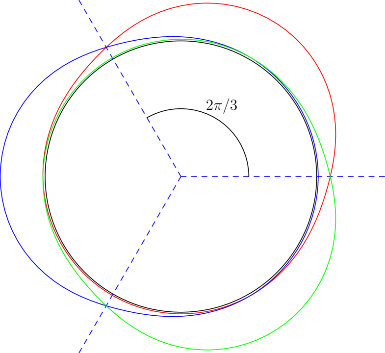
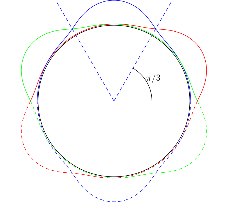
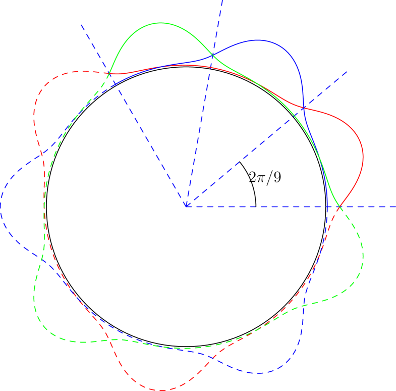
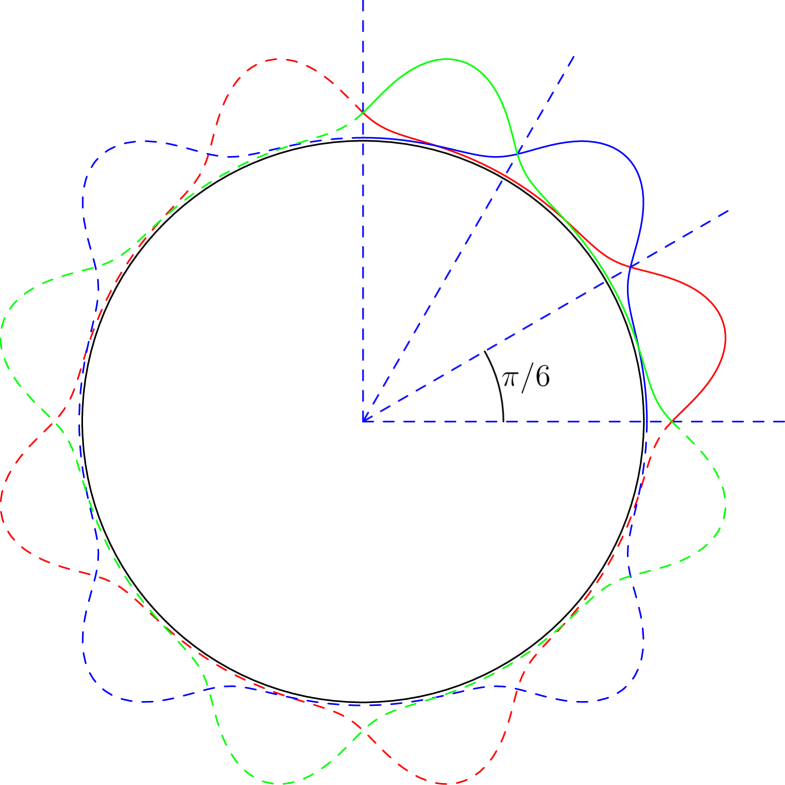
Figure 1. In the figure we represent some of the solutions obtained in Theorem 5.1. Here the number of components is set as $k=3$: each component is drawn with a different color. On the other hand the periodicity (that is, how many times the patch of $3$-components is replicated in the circle) is given by $h=1$ (up left), $h=2$ (up right), $h=3$ (down left) and $h=4$ (down right), respectively. As a consequence, the growth rate $d$ varies as $d=\frac{3}{2},3,\frac{9}{2},6$, following the same order.

Remark 5.2.

We point out that the symmetries (5.1) implies that $u_{1}^{d}$ is symmetric with respect to the reflection with the axis $y=\tan\left(\frac{\pi}{2d}\right)x$.

For a solution $(u_{1},\dots,u_{k})$ of system (1.4) in $\mathbb{R}^{2}$, we introduce the functionals

(5.3) $$\begin{split}E^{alg}(r;\Lambda)&:=\int_{B_{r}}\sum_{i=1}^{k}|\nabla u_{i}|^{2}+\Lambda\sum_{1\leq i<j\leq k}\left(u_{i}u_{j}\right)^{2}\\ H^{alg}(r)&:=\frac{1}{r}\int_{\partial B_{r}}\sum_{i=1}^{k}\left(u_{i}\right)^{2}\end{split}$$

The index $alg$ denotes the fact that these quantities are well suited to describe the growth of $(u_{1},\dots,u_{k})$ under the assumption that $(u_{1},\dots,u_{k})$ has algebraic growth. In particular, as proved in Lemma 2.1 of [6] and Corollary A.8 of [7] for the case $k=2$, the Almgren quotient

$$N^{alg}(r;1):=\frac{E^{alg}(r;1)}{H^{alg}(r)}$$

is bounded in $r\in\mathbb{R}^{+}$ if and only if $(u_{1},\dots,u_{k})$ has algebraic growth.

It is not difficult to adapt the proof of Proposition 5.2 in [2] to obtain the following general result (in the sense that it holds true for an arbitrary solution of (1.4) in $\mathbb{R}^{N}$, for any dimension $N\geq 2$).

Proposition 5.3 (see Proposition 5.2 of [2]).

Let $N\geq 2$,

$$\Lambda\in\begin{cases}\left[1,\frac{N}{N-2}\right]&\text{if $N>2$}\\ \left[1,+\infty\right)&\text{if $N=2$},\end{cases}$$

and let $(u_{1},\ldots,u_{k})$ be a solution of (1.4) in $\mathbb{R}^{N}$; the Almgren quotient

$$N^{alg}(r;\Lambda):=\frac{E^{alg}(r;\Lambda)}{H^{alg}(r)}=\frac{\displaystyle r\int_{B_{r}}\sum_{i=1}^{k}|\nabla u_{i}|^{2}+\Lambda\sum_{1\leq i<j\leq k}\left(u_{i}u_{j}\right)^{2}}{\displaystyle\int_{\partial B_{r}}\sum_{i=1}^{k}\left(u_{i}\right)^{2}},$$

is well defined in $(0,+\infty)$ and nondecreasing in $r$.

Proof.

We observe that

(5.4) $$\begin{split}\frac{\mathrm{d}missing}{\mathrm{d}r}E^{alg}(r;\Lambda)&=\frac{\mathrm{d}missing}{\mathrm{d}r}\left(\frac{1}{r^{N-2}}\int_{B_{r}}\sum_{i}|\nabla u_{i}|^{2}+\sum_{i<j}\left(u_{i}u_{j}\right)^{2}\right)+\frac{\mathrm{d}missing}{\mathrm{d}r}\left(\frac{\Lambda-1}{r^{N-2}}\int_{B_{r}}\sum_{i<j}\left(u_{i}u_{j}\right)^{2}\right)\\ &=\frac{2}{r^{N-2}}\int_{\partial B_{r}}\sum_{i}(\partial_{\nu}u_{i})^{2}+\frac{2}{r^{N-1}}\int_{B_{r}}\sum_{i<j}\left(u_{i}u_{j}\right)^{2}\\ &\qquad+\frac{(2-N)(\Lambda-1)}{r^{N-1}}\int_{B_{r}}\sum_{i<j}u_{i}^{2}u_{j}^{2}+\frac{\Lambda-1}{r^{N-2}}\int_{\partial B_{r}}\sum_{i<j}u_{i}^{2}u_{j}^{2},\end{split}$$

where we used equation (5.3) in [2]. Proceeding as in the proof of Proposition 5.2 in [2], one gets

$$\begin{split}\frac{\mathrm{d}missing}{\mathrm{d}r}N^{alg}(r;\Lambda)\geq(2+(\Lambda-1)(2-N))\frac{\int_{B_{r}}\sum_{i<j}u_{i}^{2}u_{j}^{2}}{r^{N-1}H^{alg}(r)}+\frac{(\Lambda-1)\int_{\partial B_{r}}\sum_{i<j}u_{i}^{2}u_{j}^{2}}{r^{N-2}H^{alg}(r)},\end{split}$$

which is $\geq 0$ by our assumption on $\Lambda$. ∎

Remark 5.4.

In [2] the authors consider the case $\Lambda=1$.

We work in the plane $\mathbb{R}^{2}$, so that it is possible to choose $\Lambda=2$ in Proposition 5.3. We denote $E_{d}(\cdot;\Lambda)$ and $H_{d}$ the quantities defined in (5.3) when referred to the functions $(u_{1}^{d},\ldots,u_{k}^{d})$ defined in Theorem 5.1; also, we denote $\displaystyle N_{d}(\cdot;\Lambda):=\frac{E_{d}(\cdot;\Lambda)}{H_{d}}$. In case $\Lambda=2$, we will simply write $E_{d}$ and $N_{d}$ to ease the notation.

Lemma 5.5.

Let $(u_{1}^{d},\ldots,u_{k}^{d})$ be defined in Theorem 5.1. There holds $\lim_{r\to+\infty}N_{d}(r)=d$.

Proof.

It is an easy consequence of the (5.2) and of Corollary 5.8 in [2], where it is proved that for the solution $(u_{1}^{d},\ldots,u_{k}^{d})$ there holds

$$\lim_{r\to+\infty}\frac{E_{d}(r;2)}{r^{2d}}=\lim_{r\to+\infty}\frac{E_{d}(r;1)}{r^{2d}}.$$

Therefore,

$$\lim_{r\to+\infty}N_{d}(r) =\lim_{r\to+\infty}\frac{E_{d}(r;2)}{H_{d}(r)}=\lim_{r\to+\infty}\frac{E_{d}(r;2)}{r^{2d}}\cdot\lim_{r\to+\infty}\frac{r^{2d}}{H_{d}(r)}$$

$$=\lim_{r\to+\infty}\frac{E_{d}(r;1)}{r^{2d}}\cdot\lim_{r\to+\infty}\frac{r^{2d}}{H_{d}(r)}=\lim_{r\to+\infty}N_{d}(r;1)=d.\qed$$

As a consequence, the following doubling property holds true:

Proposition 5.6 (See Proposition 5.3 of [2]).

For any $0<r_{1}<r_{2}$ it holds

$$\frac{H_{d}(r_{2})}{r_{2}^{2d}}\leq\frac{H_{d}(r_{1})}{r_{1}^{2d}}.$$

Proof.

A direct computation shows that

$$\frac{\mathrm{d}missing}{\mathrm{d}r}\log\frac{H_{d}(r)}{r^{2d}}=\frac{2N_{d}(r)}{r}-\frac{2d}{r}\leq 0;$$

an integration gives the thesis. ∎

Let us consider the scaling

(5.5) $$(u_{1,R}^{d},\dots,u_{k,R}^{d}):=\left(\frac{2d}{kH_{d}(R)}\right)^{\frac{1}{2}}\left(u_{1}^{d}(Rx,Ry),\dots,u_{k}^{d}(Rx,Ry)\right),$$

where $R$ will be determined later as a function of $d$. We see that

(5.6) $$\begin{cases}\displaystyle-\Delta u_{i,R}^{d}=-\beta_{R}^{d}\,u_{i,R}^{d}\sum_{j\neq i}\left(u_{j,R}^{d}\right)^{2}&\text{in $\mathbb{R}^{2}$}\\ \displaystyle\int_{\partial B_{1}}\sum_{i=1}^{k}\left(u_{i,R}^{d}\right)^{2}=\frac{2d}{k}\end{cases}$$

where $\beta_{R}^{d}:=\frac{k}{2d}H_{d}(R)R^{2}$.

Remark 5.7.

As a function of $R$, $\beta^{d}_{R}$ is continuous and such that $\beta_{R}^{d}\to 0$ if $R\to 0$ and $\beta_{R}^{d}\to\infty$ if $R\to\infty$.

Accordingly with our scaling, we introduce the new Almgren quotient

$$N_{d,R}(r):=\frac{E_{d,R}(r)}{H_{R}(r)}=\frac{\displaystyle r\int_{B_{r}}\sum_{i=1}^{k}|\nabla u_{i,R}^{d}|^{2}+2\beta_{R}^{d}\sum_{1\leq i<j\leq k}\left(u_{i,R}^{d}\,u_{j,R}^{d}\right)^{2}}{\displaystyle\int_{\partial B_{r}}\sum_{i=1}^{k}\left(u_{i,R}^{d}\right)^{2}}.$$

We point out that $N_{d,R}(r)=N_{d}(Rr)$, so that from Lemma 5.5 and the monotonicity of $N_{d}$ we deduce

(5.7) $$N_{d,R}(r)\leq d\qquad\forall r,R>0,$$

for every $d$. By the symmetries, the solution $(u_{1,R}^{d},\dots,u_{k,R}^{d})$ is $\frac{k\pi}{d}$-periodic with respect to the angular component, thus it is convenient to restrict our attention to the cones

$$S^{d}_{r}:=\left\{(\rho,\theta):\rho\in(0,r),\theta\in\left(0,\frac{k\pi}{d}\right)\right\}\quad\text{and}\quad S^{d}:=\left\{(\rho,\theta);\rho>0,\theta\in\left(0,\frac{k\pi}{d}\right)\right\}.$$

The boundary $\partial S^{d}_{r}$ can be decomposed as $\partial S^{d}_{r}=\partial_{p}S^{d}_{r}\cup\partial_{r}S^{d}_{r}$, where

$$\partial_{p}S^{d}_{r}:=(0,r)\times\left\{0,\frac{k\pi}{d}\right\}\quad\text{and}\quad\partial_{r}S^{d}_{r}:=\{r\}\times\left(0,\frac{k\pi}{d}\right).$$

Taking into account the periodicity of $(u_{1,R}^{d},\ldots,u_{k,R}^{d})$, we note that $(u_{1,R}^{d},\ldots,u_{k,R}^{d})$ has periodic boundary conditions on $\partial_{p}S^{d}_{r}$; furthermore

(5.8) $$\begin{split}E_{d,R}(r)&=\frac{2d}{k}\int_{S^{d}_{r}}\sum_{i}|\nabla u_{i,R}^{d}|^{2}+2\beta_{R}^{d}\sum_{i<j}\left(u_{i,R}^{d}\,u_{j,R}^{d}\right)^{2}\\ H_{d,R}(r)&=\frac{2d}{kr}\int_{\partial_{r}S^{d}_{r}}\sum_{i}\left(u_{i,R}^{d}\right)^{2}\\ N_{d,R}(r)&=\frac{\displaystyle r\int_{S^{d}_{r}}\sum_{i}|\nabla u_{i,R}^{d}|^{2}+2\beta_{R}^{d}\sum_{i<j}\left(u_{i,R}^{d}\,u_{j,R}^{d}\right)^{2}}{\displaystyle\int_{\partial S^{d}_{r}}\sum_{i}\left(u_{i,R}^{d}\right)^{2}}.\end{split}$$

5.2. A blow-up in a neighborhood of $(1,0)$

In order to pursue our strategy, we consider the further scaling

(5.9) $$(\hat{u}_{1,R}^{d}(x,y),\dots,\hat{u}_{k,R}^{d}(x,y))=\frac{\sqrt{\beta_{R}^{d}}}{d}\left(u_{1,R}^{d}\left(1+\frac{x}{d},\frac{y}{d}\right),\dots,u_{k,R}^{d}\left(1+\frac{x}{d},\frac{y}{d}\right)\right).$$

Accordingly, we will consider the scaled domains $\hat{S}^{d}_{r}=d\left(S^{d}_{r}-(1,0)\right)$ and $\hat{S}^{d}=d\left(S^{d}-(1,0)\right)$ and the respective boundaries. Having in mind to let $d\to\infty$, we observe that this scaling is a blow-up centered in the point $(1,0)$. It is easy to verify that $(\hat{u}_{1,R}^{d},\ldots,\hat{u}_{k,R}^{d})$ solves (see (5.6))

(5.10) $$\begin{cases}\displaystyle-\Delta\hat{u}_{i,R}^{d}=-\hat{u}_{i,R}^{d}\sum_{j\neq i}\left(\hat{u}_{j,R}^{d}\right)^{2}&\text{in $\hat{S}^{d}$}\\ \displaystyle\int_{\partial_{r}\hat{S}^{d}_{1}}\sum_{i=1}^{k}\left(\hat{u}_{i,R}^{d}\right)^{2}=\frac{2\beta_{R}^{d}}{k},\end{cases}$$

with suitable periodic conditions on $\partial\hat{S}^{d}$. A direct computation shows that from (5.8) it follows

$$N_{d,R}(r)=d\frac{\displaystyle r\int_{\hat{S}^{d}_{r}}\sum_{i}|\nabla\hat{u}_{i,R}^{d}|^{2}+2\sum_{i<j}\left(\hat{u}_{i,R}^{d}\hat{u}_{j,R}^{d}\right)^{2}}{\displaystyle\int_{\partial_{r}\hat{S}^{d}_{r}}\sum_{i}\left(\hat{u}_{i,R}^{d}\right)^{2}},$$

where in the new coordinates

(5.11) $$r=\sqrt{\left(1+\frac{x}{d}\right)^{2}+\left(\frac{y}{d}\right)^{2}}.$$

We are then led to define a new Almgren quotient for the scaled functions $(\hat{u}_{1,R}^{d},\ldots,\hat{u}_{k,R}^{d})$:

$$\begin{split}\hat{E}_{d,R}(r)&:=\int_{\hat{S}^{d}_{r}}\sum_{i=1}^{k}|\nabla\hat{u}_{i,R}^{d}|^{2}+2\sum_{1\leq i<j\leq k}\left(\hat{u}_{i,R}^{d}\hat{u}_{j,R}^{d}\right)^{2}\\ \hat{H}_{d,R}(r)&:=\frac{1}{r}\int_{\partial_{r}\hat{S}^{d}_{r}}\sum_{i=1}^{k}\left(\hat{u}_{i,R}^{d}\right)^{2}\\ \hat{N}_{d,R}(r)&:=\frac{\hat{E}_{d,R}(r)}{\hat{H}_{d,R}(r)}=\frac{1}{d}N_{d,R}(r).\end{split}$$

From the equation (5.7), we deduce

(5.12) $$\hat{N}_{d,R}(r)\leq 1\qquad\forall r,R>0,\ \forall d\in\frac{\mathbb{N}}{2}.$$

In order to understand the behavior of $(\hat{u}_{1,R}^{d},\ldots,\hat{u}_{k,R}^{d})$ when $d\to\infty$, we fix $R=R(d)$ to get a non-degeneracy condition.

Lemma 5.8.

For every $d\in\frac{\mathbb{N}}{2}$ there exists $R_{d}>0$ such that

$$\hat{H}_{d,R_{d}}(1)=\int_{\partial_{r}\hat{S}_{1}^{d}}\sum_{i}\left(\hat{u}_{i,R_{d}}^{d}\right)^{2}=1.$$

Proof.

By (5.10) we know that $\hat{H}_{d}(1)=\frac{2\beta_{R}^{d}}{k}$, so that we have to find $R_{d}$ such that $\beta_{R}^{d}=\frac{k}{2}$. As observed in Remark 5.7, this choice is possible. ∎

We denote $(\hat{u}_{1}^{d},\ldots,\hat{u}_{k}^{d}):=(\hat{u}_{1,R_{d}}^{d},\ldots,\hat{u}_{k,R_{d}}^{d})$, $\hat{H}_{d}:=\hat{H}_{d,R_{d}}$, $\hat{E}_{d}:=\hat{E}_{d,R_{d}}$, $\hat{N}_{d}:=\hat{N}_{d,R_{d}}$ and $\beta^{d}:=\beta^{d}_{R_{d}}$. We aim at proving that , up to a subsequence, the family $\left\{(\hat{u}_{1}^{d},\dots,\hat{u}_{k}^{d}):\ d\in\frac{\mathbb{N}}{2}\right\}$ converges, as $d\to+\infty$, to a solution of (1.4). To this aim, major difficulties arise from the fact that $\hat{S}^{d}_{r}$ and $\hat{S}^{d}$ depend on $d$; in the next Lemma we show that this problem can be overcome thanks to a convergence property of these domains.

Lemma 5.9.

For any $r>1$, the sets $\hat{S}^{d}_{r}$ converge to $\mathbb{R}\times(0,k\pi)$ as $k\to+\infty$, in the sense that

$$\mathbb{R}\times(0,k\pi)=\operatorname{Int}\left(\bigcap_{n\in\frac{\mathbb{N}}{2}}\bigcup_{d>n}\hat{S}^{d}_{r}\right),$$

where for $A\subset\mathbb{R}^{2}$ we mean that $\operatorname{Int}(A)$ denotes the inner part $A$. Analogously,

$$\mathbb{R}\times(0,k\pi)=\operatorname{Int}\left(\bigcap_{n\in\frac{\mathbb{N}}{2}}\bigcup_{d>n}\hat{S}^{d}\right)\quad\text{and}\quad(-\infty,0)\times(0,k\pi)=\operatorname{Int}\left(\bigcap_{n\in\frac{\mathbb{N}}{2}}\bigcup_{d>n}\hat{S}^{d}_{1}\right),$$

and for every $\bar{x}\in\mathbb{R}$

$$(-\infty,\bar{x})\times(0,k\pi)=\operatorname{Int}\left(\bigcap_{n\in\frac{\mathbb{N}}{2}}\bigcup_{d>n}\hat{S}^{d}_{1+\frac{\bar{x}}{d}}\right).$$

Proof.

We prove only the first claim. Let $r>1$.

Step 1)

$\displaystyle\mathbb{R}\times(0,k\pi)\subset\bigcap_{n\in\frac{\mathbb{N}}{2}}\bigcup_{d>n}\hat{S}^{d}_{r}$.
Let $(x,y)\in\mathbb{R}\times(0,k\pi)$. We show that for every $d\in\frac{\mathbb{N}}{2}$ sufficiently large $(x,y)\in\hat{S}_{r}^{d}$, that is, $\left(1+\frac{x}{d},\frac{y}{d}\right)\in S^{d}_{r}$, which means

$$\sqrt{\left(1+\frac{x}{d}\right)^{2}+\left(\frac{y}{d}\right)^{2}}<r\quad\text{and}\quad\arctan\left(\frac{y}{x+d}\right)\in\left(0,\frac{k\pi}{d}\right).$$

For the first condition it is possible to choose $d$ sufficiently large, as $r>1$. To prove the second condition, we start by considering $d>-x$, so that $\arctan\left(\frac{y}{x+d}\right)>0$. Now, provided $d$ is sufficiently large

$$\arctan\left(\frac{y}{x+d}\right)<\frac{k\pi}{d}\quad\Leftrightarrow\quad y<(x+d)\tan\left(\frac{k\pi}{d}\right).$$

Since $y<k\pi$, there exists $\varepsilon>0$ such that $y\leq k(1-\varepsilon)\pi$. Let $\bar{d}$ be sufficiently large so that

$$x+d>\left(1-\frac{\varepsilon}{2}\right)d\quad\text{and}\quad\frac{d}{k\pi}\tan\left(\frac{k\pi}{d}\right)>1-\frac{\varepsilon}{2}$$

for every $d>\bar{d}$. Then

$$(x+d)\tan\left(\frac{k\pi}{d}\right)>\left(1-\frac{\varepsilon}{2}\right)^{2}k\pi>(1-\varepsilon)k\pi\geq y$$

whenever $d>\bar{d}$.

Step 2)

$\displaystyle\bigcap_{n\in\frac{\mathbb{N}}{2}}\bigcup_{d>n}\hat{S}^{d}_{r}\subset\mathbb{R}\times[0,k\pi]$.
We show that $\left(\mathbb{R}\times[0,k\pi]\right)^{c}\subset\left(\bigcap_{n\in\frac{\mathbb{N}}{2}}\bigcup_{d>n}\hat{S}^{d}_{r}\right)^{c}$. If $(x,y)\not\in\mathbb{R}\times[0,k\pi]$, then $y>k\pi$ or $y<0$. We consider only the case $y>k\pi$; in such a situation

$$y>k\pi=\lim_{d\to\infty}(x+d)\tan\left(\frac{k\pi}{d}\right),$$

so that $(x,y)\not\in\hat{S}^{d}_{r}$ for every $d$ sufficiently large. ∎

Remark 5.10.

As a consequence of the previous result, we see that

$$\partial_{r}\hat{S}^{d}_{1}\to\{0\}\times[0,k\pi]\quad\text{and}\quad\partial_{r}\hat{S}^{d}_{1+\frac{\bar{x}}{d}}\to\{\bar{x}\}\times[0,k\pi]$$

for every $\bar{x}\in\mathbb{R}$.

Figure 2. Visualization of the construction in Lemma 5.9. In red the limiting set $\mathbb{R}\times(0,k\pi)$. In blue some of the scaled domains $\hat{S}^{d}_{r}$, for $r>1$.

Remark 5.11.

Recall the expression of $r$ in the new variable, given by (5.11). For every $r>0$ and $d\in\frac{\mathbb{N}}{2}$ there exists $\xi(r,d)$ such that

$$r=1+\frac{\xi(r,d)}{d}\quad\Leftrightarrow\quad\xi(r,d)=d(r-1).$$

Note that for every $(x,y)\in\partial_{r}\hat{S}_{r}^{d}$ it results $x<\xi(r,d)$. On the contrary, fixing $(x,y)\in\partial_{r}\hat{S}_{r}^{d}$ there exists $\zeta(d,x,y)$ such that

$$r=\sqrt{\left(1+\frac{x}{d}\right)^{2}+\left(\frac{y}{d}\right)^{2}}=1+\frac{x}{d}+\zeta(d,x,y).$$

In particular, if $y=0$ we have $\zeta(d,x,0)=0$, while if $y>0$, $\zeta(d,x,y)\sim d^{-2}$.

We are ready to prove the convergence of $\{(\hat{u}_{1}^{d},\dots,\hat{u}_{k}^{d})\}$ as $d\to\infty$.

Lemma 5.12.

Up to a subsequence, $\{(\hat{u}_{1}^{d},\dots,\hat{u}_{k}^{d})\}$ converges in $\mathcal{C}^{2}_{loc}\left(C_{\infty}\right)$, as $d\to\infty$, to a nontrivial solution $(\hat{u}_{1},\dots,\hat{u}_{k})$ of (1.4). This solution, which is $k\pi$-periodic in $y$, enjoys the symmetries

$$\hat{u}_{i+1}(x,y)=\hat{u}_{i}\left(x,y-\pi\right)\quad\text{and}\quad\hat{u}_{1}\left(x,y+\frac{\pi}{2}\right)=\hat{u}_{1}\left(x,y-\frac{\pi}{2}\right)$$

Proof.

From Proposition 5.6 and Lemma 5.8, we deduce that for any $r\geq 1$ and $d$ the inequality

$$\frac{\hat{H}_{d}(r)}{r^{2d}}=\frac{\beta^{d}H_{d}(r)}{d^{2}r^{2d}}\leq\frac{\beta^{d}}{d^{2}}H_{d}(1)=\hat{H}_{d}(1)=1$$

holds. For every $x>0$, let $r=1+\frac{x}{d}$; for every $d$ sufficiently large, we have

(5.13) $$\hat{H}_{d}\left(1+\frac{x}{d}\right)\leq\left(1+\frac{x}{d}\right)^{2d}\leq 2e^{2x}$$

Recalling the (5.12) (which we apply for $R=R_{d}$), we deduce

(5.14) $$\hat{E}_{d}\left(1+\frac{x}{d}\right)=\hat{N}_{d}\left(1+\frac{x}{d}\right)\hat{H}_{d}\left(1+\frac{x}{d}\right)\leq 2e^{2x}$$

for every $d$ sufficiently large. Recall that $(\hat{u}_{1}^{d},\dots,\hat{u}_{k}^{d})$ can be extended by angular periodicity in the whole plane $\mathbb{R}^{2}$. Let us introduce

$$T_{r}^{d}:=\left\{(\rho,\theta):\rho<r,\ \theta\in\left(-\frac{\pi}{d},(k+1)\frac{\pi}{d}\right)\right\}\supset S_{r}^{d},$$

and let $\hat{T}_{r}^{d}:=d\left(T_{r}^{d}-(1,0)\right)\supset\hat{S}_{r}^{d}$. Suitably modifying the argument in Lemma 5.9, it is not difficult to see that

$$\operatorname{Int}\left(\bigcap_{n\in\frac{\mathbb{N}}{2}}\bigcup_{d>n}\hat{T}_{1+\frac{\bar{x}}{d}}^{d}\right)=(-\infty,\bar{x})\times(-\pi,(k+1)\pi)$$

for every $\bar{x}\in\mathbb{R}$. Hence, let $B$ an open ball contained in $\mathbb{R}\times(-\pi,(k+1)\pi)$, and let $x_{B}:=\sup\{x:(x,y)\in B\}$, so that $B\subset(-\infty,x_{B}+1)\times(-\pi,(k+1)\pi)$. Using the same argument in the proof of Lemma 5.9, it is possible to show that

$$B\subset\hat{T}_{r}^{d},$$

for every $d$ sufficiently large, and by the (5.14) and the periodicity of $(\hat{u}_{1},\dots,\hat{u}_{k})$ we deduce

$$\int_{B}\sum_{i}|\nabla u_{i}|^{2}\leq 3\hat{E}_{d}\left(1+\frac{x_{B}+1}{d}\right)\leq 2e^{2(x_{B}+1)}$$

whenever $d$ is sufficiently large. This, together with (5.13), implies that $\{(\hat{u}_{1}^{d},\ldots,\hat{u}_{k}^{d})\}$ is uniformly bounded in $H^{1}(B)$, for every $B\subset\mathbb{R}\times(-\pi,(k+1)\pi)$. By the compactness of the trace operator, this bound provides a uniform-in-$d$ bound on the $L^{2}(\partial K)$ norm for every compact $K\subset\subset\mathbb{R}\times(-\pi,(k+1)\pi)$, which in turns, due to the subharmonicity of $u_{i}^{d}$, gives a uniform-in-$d$ bound on the $L^{\infty}(K)$ norm of $\{(\hat{u}_{1}^{d},\ldots,\hat{u}_{k}^{d})\}$, for every compact set $K\subset\subset\mathbb{R}\times(-\pi,(k+1)\pi)$. The standard regularity theory for elliptic equations guarantees that when $d\to\infty$ then $\{(\hat{u}_{1}^{d},\ldots,\hat{u}_{k}^{d})\}$ converges in $\mathcal{C}^{2}_{loc}(\mathbb{R}\times(-\pi,(k+1)\pi))$, up to a subsequence, to a function $(\hat{u}_{1},\dots,\hat{u}_{k})$ which is a solution to (1.4). By the convergence and by the normalization required in Lemma 5.8, we deduce that (recall also the convergence of the boundaries $\partial\hat{S}_{1}^{d}$, Remark 5.10)

$$\int_{0}^{k\pi}\sum_{i}\hat{u}_{i}(0,y)^{2}\,\mathrm{d}y=1;$$

in particular, $(\hat{u}_{1},\dots,\hat{u}_{k})$ is nontrivial. The $k\pi$-periodicity in $y$ follows directly form the convergence of the domains, Lemma 5.9. By the pointwise convergence of $(\hat{u}_{1}^{d},\dots,\hat{u}_{k}^{d})$ to $(\hat{u}_{1},\dots,\hat{u}_{k})$ and by the symmetries of each function $(\hat{u}_{1}^{d},\dots,\hat{u}_{k}^{d})$ (see equation (5.1) and Remark 5.2) we deduce also that

$$\hat{u}_{i+1}(x,y)=\hat{u}_{i}\left(x,y-\pi\right)\quad\text{and}\quad\hat{u}_{1}\left(x,y+\frac{\pi}{2}\right)=\hat{u}_{1}\left(x,y-\frac{\pi}{2}\right).$$

∎

5.3. Characterization of the growth of $(\hat{u}_{1},\dots,\hat{u}_{k})$

So far we proved the existence of a solution $(\hat{u}_{1},\dots,\hat{u}_{k})$ of (1.4) which enjoys the properties 1) and 2) of Theorem 1.8. In this subsection, we are going to complete the proof of the quoted statement, showing that $(\hat{u}_{1},\dots,\hat{u}_{k})$ enjoys also the properties 3)-5). We denote as $\hat{\mathcal{E}},\hat{E},\hat{H}$ and $\hat{N}$ the quantities $\mathcal{E}^{unb},E^{unb},H$ and $N^{unb}$ introduced in subsection 2.2 when referred to the function $(\hat{u}_{1},\ldots,\hat{u}_{k})$. Firstly, we show that $(\hat{u}_{1},\dots,\hat{u}_{k})$ has finite energy, point 3) of Theorem 1.8, and that $\hat{H}(x)\to-\infty$ as $x\to-\infty$.

Lemma 5.13.

For every $x\in\mathbb{R}$ there holds $\hat{\mathcal{E}}(x)<+\infty$. In particular

$$\hat{\mathcal{E}}(x)\leq\liminf_{d\to\infty}\hat{\mathcal{E}}_{d}\left(1+\frac{x}{d}\right)\quad\text{and}\quad\hat{E}(x)\leq\liminf_{d\to\infty}\hat{E}_{d}\left(1+\frac{x}{d}\right).$$

Furthermore, $\displaystyle\lim_{x\to-\infty}\hat{H}(x)=0$.

Proof.

By the $\mathcal{C}^{2}_{loc}(\mathbb{R}^{2})$ convergence of $(\hat{u}_{1}^{d},\dots,\hat{u}_{k}^{d})$ to $(\hat{u}_{1},\dots,\hat{u}_{k})$ and by the convergence properties of the domains $\hat{S}^{d}_{1+\frac{x}{d}}$, Lemma 5.9, we deduce

$$\lim_{d\to\infty}\left(\sum_{i}|\nabla\hat{u}_{i}^{d}|^{2}+\sum_{i<j}\left(\hat{u}_{i}^{d}\hat{u}_{j}^{d}\right)^{2}\right)\chi_{\hat{S}_{1+\frac{x}{d}}^{d}}=\left(\sum_{i}|\nabla\hat{u}_{i}|^{2}+\sum_{i<j}\left(\hat{u}_{i}\hat{u}_{j}\right)^{2}\right)\chi_{C_{(-\infty,x)}}\qquad\text{a. e. in $C_{\infty}$},$$

for every $x\in\mathbb{R}$. As a consequence, we can apply the Fatou lemma obtaining

$$\hat{\mathcal{E}}(x)\leq\liminf_{d\to\infty}\hat{\mathcal{E}}_{d}\left(1+\frac{x}{d}\right)\leq 2e^{2x},$$

where the uniform boundedness of $\hat{\mathcal{E}}_{d}\left(1+\frac{x}{d}\right)$ comes from (5.14). To prove that $\hat{H}(x)\to 0$ as $x\to-\infty$, we can proceed with the same argument developed in Lemma 4.7. ∎

In light of the previous Lemma, the monotonicity formulae proved in subsection 2.2 applies for $\hat{\mathcal{E}},\hat{E},\hat{H}$ and $\hat{N}$.

Lemma 5.14.

There holds

$$\lim_{x\to+\infty}\hat{N}(x)=1.$$

Proof.

By Proposition 2.14, we know that $\hat{N}$ is nondecreasing in $x$, and thanks to the symmetries of $(\hat{u}_{1},\dots,\hat{u}_{k})$, see Lemma 5.12, Lemma 2.17 implies that $\lim_{x\to+\infty}\hat{N}(x)\geq 1$. It remains to show that this limit is smaller then $1$. This follows from the estimates of Lemma 5.13 and from the strong convergence of $(\hat{u}_{1}^{d},\dots,\hat{u}_{k}^{d})\to(\hat{u}_{1},\dots,\hat{u}_{k})$, which implies that $\hat{H}_{d}\left(1+\frac{x}{d}\right)\to\hat{H}(x)$ as $d\to\infty$: therefore, for every $x\in\mathbb{R}$

$$\hat{N}(x)=\frac{\hat{E}(x)}{\hat{H}(x)}\leq\frac{\liminf_{d\to\infty}\hat{E}_{d}(x)}{\lim_{d\to\infty}\hat{H}_{d}(x)}=\liminf_{d\to\infty}\hat{N}_{d}(x)\leq 1,$$

where we used the (5.12). ∎

In light of this achievement, we can apply Corollary 2.15 to complete the proof of point 5) of Theorem 1.8. The fact that $\gamma>0$ follows by Lemmas 5.14 and 2.17):

$$\lim_{r\to+\infty}\frac{\hat{H}(r)}{e^{2r}}=\lim_{r\to+\infty}\frac{\hat{E}(r)}{e^{2r}}\cdot\lim_{r\to+\infty}\frac{1}{\hat{N}(r)}>0.$$

Remark 5.15.

With a similar construction, it is possible to obtain the existence of solutions to (1.4) in $\mathbb{R}^{2}$ modeled on $\cosh x\sin y$. To do this, we can first construct solutions of (1.4) having algebraic growth defined outside the ball of radius $1$, with homogeneous Neumann boundary conditions on $\partial B_{1}$. This can be done suitably modifying the proof of Theorem 1.6 in [2]. Then, performing a new blow-up in a neighborhood of $(1,0)$, we can obtain a solution of (1.4) defined in $\mathbb{R}_{+}^{2}$, with homogeneous Neumann condition on $\{x=0\}$; this solution can be extended by even-symmetry in $x$ in the whole $\mathbb{R}^{2}$.

6. Asymptotics of solutions which are periodic in one variable

In this section we prove Theorem 1.9.

Proof of Theorem 1.9.

Let us start with case ($i$). First of all, let us recall that, since the solution $(u,v)$ is non trivial, $N(0)>0$: in particular, from point ($i$) of Corollary 2.15 it follows that $H(r)\to+\infty$ as $r\to+\infty$. Let us consider the shifted functions

$$(u_{R}(x,y),v_{R}(x,y)):=\frac{1}{\sqrt{H(R)}}(u(x+R,y),v(x+R,y))$$

which solve the system

$$\begin{cases}-\Delta u_{R}=-H(R)u_{R}v_{R}^{2}&\text{in $C_{\infty}$}\\ -\Delta v_{R}=-H(R)u_{R}^{2}v_{R}&\text{in $C_{\infty}$}\\ \displaystyle\int_{\Sigma_{0}}u_{R}^{2}+v_{R}^{2}=1\end{cases}$$

and share the same periodicity of $(u,v)$. We introduce

$$\begin{split}E_{R}(r):=\int_{C_{(-\infty,r)}}|\nabla u_{R}|^{2}+|\nabla_{R}|^{2}+2H(R)u_{R}^{2}v_{R}^{2},\\ H_{R}(r):=\int_{\Sigma_{r}}u_{R}^{2}+v_{R}^{2}\quad\text{and}\quad N_{R}(r):=\frac{E_{R}(r)}{H_{R}(r)}.\end{split}$$

It is easy to see that

$$\begin{split}E_{R}(r)&=\frac{1}{H(R)}E^{unb}(r+R)\\ H_{R}(r)&=\frac{1}{H(R)}H(r+R)\end{split}\quad\Rightarrow\quad N_{R}(r)=N^{unb}(r+R)$$

for any $r$ (recall that $E^{unb}$ and $N^{unb}$ have been defined in subsection 2.2). We point out that, by definition, $N_{R_{1}}(r)\leq N_{R_{2}}(r)$ for every $R_{1}<R_{2}$. Furthermore, $N_{R}(r)\leq N(+\infty)$ for every $r,R$ and $N_{R}(r)\to N(+\infty)$ as $R\to\infty$ for every $r\in\mathbb{R}$. Therefore, $N_{R}$ tends to the constant function $N(+\infty)$ in $L^{1}_{\mathrm{loc}}(\mathbb{R})$.

Thanks to the normalization condition $H_{R}(0)=1$ and the uniform bound $N_{R}(r)<N(+\infty)$, applying Corollary 2.15 (see also Remark 2.18) we deduce that $H_{R}(r)$ is uniformly bounded in $R$ for every $r>0$. Consequently, also $E_{R}(r)$ is uniformly bounded in $R$ for every $r>0$, and this reveals that the sequence $(u_{R},v_{R})$ is uniformly bounded in $H^{1}_{\mathrm{loc}}(C_{\infty})$ and, by standard elliptic estimates, in $L^{\infty}_{\mathrm{loc}}(C_{\infty})$. From Theorem 2.6 of [11] (it is a local versione of Theorem 1.1 of [9]), we evince that the sequence $(u_{R},v_{R})$ is uniformly bounded also in $\mathcal{C}^{0,\alpha}_{\mathrm{loc}}(C_{\infty})$ for any $\alpha\in(0,1)$. Consequently, up to a subsequence, $(u_{R},v_{R})$ converges in $\mathcal{C}^{0}_{loc}(C_{\infty})$ and in $H^{1}_{loc}(C_{\infty})$ to a pair $(\Psi^{+},\Psi^{-})$, where $\Psi$ is a nontrivial harmonic function (this is a combination of the main results in [9] and [5]). By the convergence, $\Psi$ has to be $2\pi$-periodic in $y$.

Firstly, we prove that $H(r;\Psi)\to 0$ ar $r\to-\infty$, so that the results of subsection 2.3 hold true for $\Psi$. As already observed, $N_{R}(r)\geq N_{\bar{R}}(r)$ for every $r\in\mathbb{R}$, for every $R>\bar{R}$. By the expression of the logarithmic derivative of $H_{R}$, see Corollary 2.15 (see also Remark 2.18) we have

$$\frac{\mathrm{d}missing}{\mathrm{d}r}\log H_{R}(r)=2N_{R}(r)\geq 2N_{\bar{R}}(r)=\frac{\mathrm{d}missing}{\mathrm{d}r}\log H_{\bar{R}}(r)\qquad\forall r.$$

As a consequence, taking into account that $H_{R}(0)=1$ for every $R$, for every $r<0$ it results

$$\frac{H_{R}(0)}{H_{R}(r)}\geq\frac{H_{\bar{R}}(0)}{H_{\bar{R}}(r)}\quad\Leftrightarrow\quad H_{\bar{R}}(r)\geq H_{R}(r)\qquad\forall R>\bar{R}.$$

Passing to the limit as $R\to+\infty$, by the $\mathcal{C}^{0}_{\mathrm{loc}}(\mathbb{R}^{2})$ convergence of $(u_{R},v_{R})$ to $(\Psi^{+},\Psi^{-})$ it follows that $H_{\bar{R}}(r)\geq H(r;\Psi)$, which gives $H(r;\Psi)\to 0$ as $r\to-\infty$ in light of our assumption on $(u,v)$.

Using again the expression of the logarithmic derivative of $H_{R}$ and $H(\cdot;\Psi)$, we deduce

$$\log\frac{H_{R}(r_{2})}{H_{R}(r_{1})}=2\int_{r_{1}}^{r_{2}}N_{R}(s)\mathrm{d}s\quad\text{and}\quad\log\frac{H(r_{2};\Psi)}{H(r_{1};\Psi)}=2\int_{r_{1}}^{r_{2}}N(s;\Psi)\mathrm{d}s,$$

where $r_{1}<r_{2}$. The left hand side of the first identity converges to the left hand side of the second identity; recalling that $N_{R}(r)\to N(+\infty)$ for every $r$, we deduce

$$\int_{r_{1}}^{r_{2}}N(s;\Psi)\mathrm{d}s=\lim_{R\to+\infty}\int_{r_{1}}^{r_{2}}N_{R}(s)\mathrm{d}s=N(+\infty)(r_{2}-r_{1})\quad\Rightarrow\quad\frac{1}{r_{2}-r_{1}}\int_{r_{1}}^{r_{2}}N(s;\Psi)\,\mathrm{d}s=N(+\infty).$$

for every $r_{1}<r_{2}$. It is well known that, being $N(\cdot;\Psi)\in L^{1}_{\mathrm{loc}}(\mathbb{R})$, the limit as $r_{2}\to r_{1}$ of the left hand side converges to $N(r_{1};\Psi)$ for almost every $r_{1}\in\mathbb{R}$. Hence, $N(r;\Psi)=N(+\infty)$ for every $r\in\mathbb{R}$. We are then in position to apply Proposition 2.21:

$$\lim_{R\to+\infty}N(R)=\lim_{R\to+\infty}N_{R}(0)=N(0;\Psi)=d\in\mathbb{N}\setminus\{0\},$$

and $\Psi(x,y)=\left[C_{1}\cos(dy)+C_{2}\sin(dy)\right]e^{dx}$ for some constant $C_{1},C_{2}\in\mathbb{R}$.

As far as case ($ii$) is concerned, for the sake of simplicity we assume $a=0$. One can repeat the proof with minor changes replacing $E^{unb}$ and $N^{unb}$ with $E^{sym}$ and $N^{sym}$ (which have been defined in subsection 2.1). The unique nontrivial step consists in proving that in this setting $H(r;\Psi)\to 0$ as $r\to-\infty$. To this aim, we note that, as before,

$$H_{R}(r)\leq H_{\bar{R}}(r)\qquad\forall R>\bar{R},$$

for every $r>-\bar{R}$. In particular, if $r>1-\bar{R}$, by Proposition 2.4 and Corollary 2.5 we deduce

$$H_{R}(r)\leq H_{\bar{R}}(r)=\frac{H(r+\bar{R})}{H(\bar{R})}\leq\frac{e^{2N(1)(r+\bar{R})}}{e^{2N(1)\bar{R}}}=e^{2N(1)r}\qquad\forall R>\bar{R},$$

for every $r>1-\bar{R}$. Passing to the limit as $R\to+\infty$, by $\mathcal{C}^{0}_{\mathrm{loc}}(\mathbb{R}^{2})$ convergence we obtain

$$H(r;\Psi)\leq e^{2N(1)r}\qquad\forall r\in\mathbb{R},$$

which yields $H(r;\Psi)\to 0$ as $r\to-\infty$. ∎

Appendix A

We start with the following version of the parabolic minimum principle, which we used in the proof of Proposition 3.1.

Lemma A.1.

Let $N\geq 2$, let $\Omega=(a,b)\times\Omega^{\prime}\subset\mathbb{R}^{N}$ be open and connected, let $c\in L^{\infty}(\Omega)$ and let $w\in H^{1}(\Omega)$ be such that

$$\begin{cases}w_{t}-\Delta w\geq c(x)w&\text{in $[0,T]\times\Omega$}\\ w\geq 0&\text{on $\{0\}\times\overline{\Omega}$}\\ w\geq 0&\text{on $(0,T)\times(a,b)\times\partial\Omega^{\prime}$},\end{cases}$$

and $w$ has $(b-a)$-periodic boundary condition on $\{a,b\}\times\Omega^{\prime}$. Then $w\geq 0$.

Proof.

Let $J(t):=\frac{1}{2}\int_{\Omega}(w^{-})^{2}$. A direct computation shows that $J^{\prime}(t)\leq 2\|c\|_{L^{\infty}(\Omega)}J(t)$, where we used the boundary conditions. Consequently,

$$J(t)\leq J(0)e^{2\|c\|_{L^{\infty}(\Omega)}t}=0\qquad\forall t\in[0,T]$$

where the last identity follows by the initial condition. ∎

Remark A.2.

Note that we do not require anything about the sign of $c$.

In sections 3 and 4, we exploited many times the following properties of the trace operators.

Theorem A.3.

For $a<b$ real numbers, let $C_{(a,b)}=(a,b)\times\mathbb{S}_{k}$ be a bounded cylinder. The trace operator $Tr:u\in H^{1}(C_{(a,b)})\mapsto u|_{\Sigma_{a}\cup\Sigma_{b}}\in L^{2}(\Sigma_{a}\cup\Sigma_{b})$ is compact.

Proof.

Let $(u_{n})\subset H^{1}(C_{(a,b)})$ be such that $u_{n}\rightharpoonup 0$. We show that $u_{n}|_{\Sigma_{a}\cup\Sigma_{b}}\to 0$ in $L^{2}(\Sigma_{a}\cup\Sigma_{b})$. For the sake of simplicity we consider the case $a=0$ and $b=1$. Let $w(x,y):=x(x-1)$. We note that $\partial_{\nu}w=1$ on $\Sigma_{0}\cup\Sigma_{1}$. Let

$$F(x,y)=\nabla w(x,y)=(2x-1,0)\quad\text{and}\quad g(x,y)=\Delta w(x,y)=2.$$

By the divergence theorem

$$2\int_{C_{(0,1)}}u_{n}^{2}=\int_{C_{(0,1)}}(\mathrm{div}F)u_{n}^{2}=-2\int_{C_{(0,1)}}2u_{n}F\cdot\nabla u_{n}+\int_{\Sigma_{a}\cup\Sigma_{b}}u_{n}^{2},$$

so that

$$\int_{\Sigma_{a}\cup\Sigma_{b}}u_{n}^{2}\leq 2\|u_{n}\|_{L^{2}(C_{(0,1)}}^{2}+2\|u_{n}\|_{L^{2}(C_{(0,1)}}\|\nabla u_{n}\|_{L^{2}(C_{(0,1)}}\to 0$$

as $n\to\infty$, by the compactness of the Sobolev embedding $H^{1}(C_{(0,1)}\hookrightarrow L^{2}(C_{(0,1)})$. ∎

Corollary A.4.

For $a<b$ real numbers, let $C_{(a,b)}=(a,b)\times\mathbb{S}_{k}$ be a bounded cylinder. The local trace operator $T_{\Sigma_{b}}:u\in H^{1}(C_{(a,b)})\mapsto u|_{\Sigma_{b}}\in L^{2}(\Sigma_{b})$ is compact.

Proof.

It is an easy consequence of Theorem A.3 and of the fact that the linear operator $L_{f}:\varphi\in L^{2}(\Sigma_{a}\cup\Sigma_{b})\mapsto f\varphi\in L^{2}(\Sigma_{a}\cup\Sigma_{b})$ is continuous for every $f\in L^{\infty}(\Sigma_{a}\cup\Sigma_{b})$. As $T_{\Sigma_{b}}=L_{\chi_{\Sigma_{b}}}\circ Tr_{C_{(a,b)}}$, where $\chi_{\Sigma_{b}}$ is the characteristic function of $\Sigma_{b}$, $T_{\Sigma_{b}}$ is compact. ∎

Acknowledgments: the authors thank Prof. Alberto Farina, Prof. Susanna Terracini and Prof. Gianmaria Verzini for many valuable discussions related to this problem. The first author is partially supported by PRIN 2009 grant ”Critical Point Theory and Perturbative Methods for Nonlinear Differential Equations”.

References

- [1] H. Berestycki, T.-C. Lin, J. Wei, and C. Zhao. On Phase-Separation Models: Asymptotics and Qualitative Properties. Arch. Ration. Mech. Anal., 208(1):163–200, 2013.
- [2] H. Berestycki, S. Terracini, K. Wang, and J. Wei. On entire solutions of an elliptic system modeling phase-separation. to appear on Adv. Math., 2013.
- [3] L. A. Caffarelli and F.-H. Lin. Singularly perturbed elliptic systems and multi-valued harmonic functions with free boundaries. J. Amer. Math. Soc., 21(3):847–862, 2008.
- [4] S.-M. Chang, C.-S. Lin, T.-C. Lin, and W.-W. Lin. Segregated nodal domains of two-dimensional multispecies Bose-Einstein condensates. Phys. D, 196(3-4):341–361, 2004.
- [5] E. N. Dancer, K. Wang, and Z. Zhang. The limit equation for the Gross-Pitaevskii equations and S. Terracini’s conjecture. J. Funct. Anal., 262(3):1087–1131, 2012.
- [6] A. Farina. Some symmetry results for entire solutions of an elliptic system arising in phase separation. Preprint, 2012.
- [7] A. Farina and N. Soave. Monotonicity and 1-dimensional symmetry for solutions of an elliptic system arising in Bose-Einstein condensation. 2013. Preprint arXiv:1303.1265.
- [8] D. Gilbarg and N. S. Trudinger. Elliptic partial differential equations of second order. Classics in Mathematics. Springer-Verlag, Berlin, 2001. Reprint of the 1998 edition.
- [9] B. Noris, H. Tavares, S. Terracini, and G. Verzini. Uniform Hölder bounds for nonlinear Schrödinger systems with strong competition. Comm. Pure Appl. Math., 63(3):267–302, 2010.
- [10] H. Tavares and S. Terracini. Regularity of the nodal set of segregated critical configurations under a weak reflection law. Calc. Var. Partial Differential Equations, 45(3-4):273–317, 2012.
- [11] K. Wang. On the De Giorgi type conjecture for an elliptic system modeling phase separation. Preprint, 2012.