FLAVOUR(267104)-ERC-38

BARI-TH/13-671

Nikhef-2013-008

UT-13-09

The Anatomy of Neutral Scalars with FCNCs in the Flavour Precision Era
Andrzej J. Buras^a,b, Fulvia De Fazio^c, Jennifer Girrbach^a,b
Robert Knegjens^d and Minoru Nagai^e
aTUM Institute for Advanced Study, Lichtenbergstr. 2a, D-85747 Garching, Germany
^bPhysik Department, TUM, James-Franck-Straße, D-85747 Garching, Germany
^cIstituto Nazionale di Fisica Nucleare, Sezione di Bari, Via Orabona 4, I-70126 Bari, Italy
^d Nikhef, Science Park 105, NL-1098 XG Amsterdam, The Netherlands
^e Department of Physics, University of Tokyo, Tokyo 113-0033, Japan

Abstract
In many extensions of the Standard Model (SM) flavour changing neutral current (FCNC) processes can be mediated by tree-level heavy neutral scalars and/or pseudo-scalars $H^{0}(A^{0})$. This generally introduces new sources of flavour violation and CP violation as well as left-handed (LH) and right-handed (RH) scalar ($1\mp\gamma_{5}$) currents. These new physics (NP) contributions imply a pattern of deviations from SM expectations for FCNC processes that depends only on the couplings of $H^{0}(A^{0})$ to fermions and on their masses. In situations in which a single $H^{0}$ or $A^{0}$ dominates NP contributions stringent correlations between $\Delta F=2$ and $\Delta F=1$ observables exist. Anticipating the Flavour Precision Era (FPE) ahead of us we illustrate this by searching for allowed oases in the landscape of a given model assuming significantly smaller uncertainties in CKM and hadronic parameters than presently available. To this end we analyze $\Delta F=2$ observables in $B^{0}_{s,d}-\bar{B}^{0}_{s,d}$ and $K^{0}-\bar{K}^{0}$ systems and rare $B$ and $K$ decays with charged leptons in the final state including both left-handed and right-handed scalar couplings of $H^{0}$ and $A^{0}$ to quarks in various combinations. We identify a number of correlations between various flavour observables that could test and distinguish these different scenarios. The prominent role of the decays $B_{s,d}\to\mu^{+}\mu^{-}$ in these studies is emphasized. Imposing the existing flavour constraints, a rich pattern of deviations from the SM expectations in rare $B_{s,d}$ decays emerges provided $M_{H}\leq 1\,{\rm TeV}$. NP effects in rare $K$ decays, except for $K_{L}\to\mu^{+}\mu^{-}$, turn out to be very small. In $K_{L}\to\mu^{+}\mu^{-}$ they can be as large as the SM contributions but due to hadronic uncertainties this is still insufficient to learn much about new scalars from this decay in the context of models considered here. Flavour violating SM Higgs contributions to rare $B_{d}$ and $K$ decays turn out to be negligible once the constraints from $\Delta F=2$ processes are taken into account. But $\mathcal{B}(B_{s}\to\mu^{+}\mu^{-})$ can still be enhanced up to $8\%$. Finally, we point out striking differences between the correlations found here and in scenarios in which tree-level FCNC are mediated by a new neutral gauge boson $Z^{\prime}$.

1 Introduction

The recent discovery of a scalar particle with a mass of $126\,{\rm GeV}$ opened the gate to the unexplored world of scalar particles which could be elementary or composite. While we will surely learn a lot about the properties of these new objects through collider experiments like ATLAS and CMS, also low energy processes, in particular flavour violating transitions, will teach us about their nature. In the Standard Model (SM) and in many of its extensions there are no fundamental flavour-violating couplings of scalars to quarks and leptons but such couplings can be generated through loop corrections leading in the case of $\Delta F=1$ transitions to Higgs-Penguins (HP) and in $\Delta F=2$ transitions to double Higgs-Penguins (DHP). However, when the masses of the scalar particles are significantly lower than the heavy new particles exchanged in the loops, the HP and DHP look at the electroweak scale as flavour violating tree diagrams. Beyond the SM such diagrams can also be present at the fundamental level, an important example being the left-right symmetric models. From the point of view of low energy theory there is no distinction between these possibilities as long as the vertices involving heavy particles in a Higgs-Penguin cannot be resolved and to first approximation what really matters is the mass of the exchanged scalar and its flavour violating couplings, either fundamental or generated at one-loop level. While all this can be formulated with the help of effective field theories and spurion technology, we find it more transparent to study directly tree diagrams with heavy particle exchanges.

In a recent paper [1] an anatomy of neutral gauge boson ($Z^{\prime}$ and $Z$) couplings to quark flavour changing neutral currents (FCNC) has been presented. Anticipating the Flavour Precision Era (FPE) ahead of us and consequently assuming significantly smaller uncertainties in CKM and hadronic parameters than presently available, it was possible to find allowed oases in the landscape of new parameters in these models and to uncover stringent correlations between $\Delta F=2$ and $\Delta F=1$ observables characteristic for such NP scenarios.

The goal of the present paper is to perform a similar analysis for scalar neutral particles and to investigate whether the patterns of flavour violation in these two different NP scenarios (gauge bosons and scalars) can be distinguished through correlations between quark flavour observables. Already at this stage it is useful to note the following differences in NP contributions to quark flavour observables in these two scenarios:

• While the lower bounds on masses of $Z^{\prime}$ gauge bosons from collider experiments are at least $1-2\,{\rm TeV}$, new neutral scalars with masses as low as a few hundred $\,{\rm GeV}$ are not excluded.

• While in the $Z^{\prime}$ scenarios in addition to new operators also SM operators with modified Wilson coefficients can be present, in the case of tree-level scalar exchanges all effective low energy operators are new.

• While there is some overlap between operators contributing to $\Delta F=2$ processes in $Z^{\prime}$ and scalar cases after the inclusion of QCD corrections, their Wilson coefficients are very different. Moreover, in $\Delta F=1$ transitions there is no overlap with the operators present in $Z^{\prime}$ models.

• Concerning flavour violating couplings of $Z$ and the SM Higgs $h$, in the case of the $Z$ boson large NP effects, in particular in rare $K$ decays, are still allowed but then its effects in $\Delta F=2$ processes turn out to be very small [1]. In the Higgs case, the smallness of the Higgs coupling to muons and electrons precludes any visible effects from tree-level Higgs exchanges in rare $K$ and $B_{d}$ decays with muon or electron pair in the final state once constraints from $\Delta F=2$ processes are taken into account. The corresponding effects in $B_{s}\to\mu^{+}\mu^{-}$ are small but can still be at the level of $8\%$. Simultaneously tree-level Higgs contributions to $\Delta F=2$ transitions can still provide in principle solutions to possible tensions within the SM.

• At first sight the couplings of scalars to neutrinos look totally negligible but if the masses of neutrinos are generated by a different mechanism than coupling to scalars, like in the case of the see-saw mechanism, it is not a priori obvious that such couplings in some NP scenarios could be measurable. Our working assumption in the present paper will be that this is not the case. Consequently NP effects of scalars in $K^{+}\rightarrow\pi^{+}\nu\bar{\nu}$, $K_{L}\rightarrow\pi^{0}\nu\bar{\nu}$ and $b\to s\nu\bar{\nu}$ transitions will be assumed to be negligible in contrast to $Z^{\prime}$ models, where NP effects in these decays could be very important [1]. As we will see, scalar contributions to $K_{L}\to\pi^{0}\ell^{+}\ell^{-}$ although in principle larger than for $K^{+}\rightarrow\pi^{+}\nu\bar{\nu}$, $K_{L}\rightarrow\pi^{0}\nu\bar{\nu}$ and $b\to s\nu\bar{\nu}$ transitions, are found to be small. In $K_{L}\to\mu^{+}\mu^{-}$ they can be as large as the SM contribution but due to hadronic uncertainties this is still insufficient to learn much about scalars from this decay, at least in the context of models considered by us.

In order to have an easy comparison with the anatomy of FCNCs mediated by a neutral gauge bosons presented in [1] the structure of the present work will be similar to the structure of the latter paper but not identical, as rare $K$ decays play in this paper a subleading role so that emphasis will be put on $B_{s}$ and $B_{d}$ systems. In Section 2 we describe our strategy by defining the relevant couplings and listing processes to be considered. Our analysis will only involve processes which are theoretically clean and have simple structure. Here we will also introduce a number of different scenarios for the scalar couplings to quarks thereby reducing the number of free parameters. In Section 3 we will first present a compendium of formulae relevant for the study of $\Delta F=2$ processes mediated by tree-level neutral scalar exchanges including for the first time NLO QCD corrections to these NP contributions. In Section 4 we discuss rare $B$ decays, in particular $B_{s,d}\to\mu^{+}\mu^{-}$. In Section 5 rare $K$ decays are considered. In Section 6 we present a general qualitative view on NP contributions to flavour observables stressing analytic correlations between $\Delta F=2$ and $\Delta F=1$ observables. In Section 7 we present our strategy for the numerical analysis and in Section 8 we execute our strategy for the determination of scalar couplings in the $B_{s}$ and $B_{d}$ systems. We discuss several scenarios for them and identify stringent correlations between various observables. We also investigate what the imposition of the $U(2)^{3}$ flavour symmetry on scalar couplings would imply. In Section 9 we present the results for rare $K$ decays, where NP effects are found to be small. In Section 10 we demonstrate that the contributions of the SM Higgs with induced flavour violating couplings, even if in principle relevant for $\Delta F=2$ transitions, are irrelevant for rare $K$ and $B_{d}$ decays with small but still visible effects in $B_{s}\to\mu^{+}\mu^{-}$. A summary of our main results and a brief outlook for the future are given in Section 11.

2 Strategy

2.1 Basic Model Assumptions

Our paper is dominated by tree-level contributions to FCNC processes mediated by a heavy neutral scalar or pseudoscalar. We use a common name, $H^{0}$, for them unless otherwise specified. When a distinction will have to be made, we will either use $H^{0}$ and $A^{0}$ for scalar and pseudoscalar, respectively or in order to distinguish SM Higgs from additional spin 0 particles we will use the familiar 2HDM and MSSM notation: $(H,A,h)$.

Our main goal is to consider the simplest extension of the SM in which the only new particle in the low energy effective theory is a single neutral particle with spin $0$ and the question arises whether this is possible from the point of view of an underlying original theory. If the scalar in question is not a $SU(2)$ singlet, then it must be placed in a complete $SU(2)$ multiplet, e.g. a second doublet as is the case of 2HDM or the MSSM. However, this implies the existence of its $SU(2)$ partners in a given multiplet with masses close to the masses of our scalar. In fact in the decoupling regime in 2HDM and MSSM the masses of $(H^{\pm},H^{0},A^{0})$ are approximately degenerate. While $SU(2)$ breaking effects in the Higgs potential allow for mass splittings, they must be of ${\cal O}(v)$ at most and consequently the case of the dominance of a single scalar is rather unlikely.

It follows then that our scalar should be a $SU(2)$ singlet. In this case, the scalar-quark couplings of $H$ come from the following low energy effective operator

$$L=\lambda_{L}^{ij}\frac{H^{0}}{\Lambda}\bar{q}_{R}^{i}q_{L}^{j}h_{\rm SM}+h.c.$$ (1)

with $\Lambda$ denoting the cut-off scale of the low energy theory. After the spontaneous breakdown of $SU(2)$ the scalar left-handed coupling is given by

$$\Delta_{L}^{ij}(H^{0})=\frac{1}{\sqrt{2}}\frac{v}{\Lambda}\lambda_{L}^{ij},$$ (2)

with analogous expression for the right-handed coupling.

Now, in the case of $\Delta F=2$ transitions the scalar contributions are governed only by the couplings $\Delta_{L,R}^{ij}(H^{0})$ to quarks and the corresponding Feynman rule has been shown in Fig 1. Here $(i,j)$ denote quark flavours. Note the following important property

$$\Delta_{L}^{ij}(H^{0})=[\Delta_{R}^{ji}(H^{0})]^{*}$$ (3)

that distinguishes it from the corresponding gauge couplings in which there is no chirality flip.

The couplings $\Delta_{L,R}^{ij}(H^{0})$ are dimensionless quantities but as these are scalar and not gauge couplings they can involve ratios of quark masses and the electroweak vacuum expectation value $v$ or other mass scales. While from the SM, 2HDM and MSSM we are used to having scalar couplings proportional to the masses of the participating quarks, it should be emphasized that this is not a general property. It applies only if the scalar and the SM Higgs, responsible for $SU(2)$ breakdown, are in the same $SU(2)$ multiplet or a multiplet of a larger gauge group $G$. Then after the breakdown of $G$ to $SU(2)$, the scalar appears as a singlet of $SU(2)$ symmetry, with couplings to quarks involving their masses after $SU(2)$ breakdown. While this is the case in several models, in our simple extension of the SM, it is more natural to think that the involved scalar couplings are unrelated to the generation of quark masses.

In spite of the last statement is useful to recall how the quark masses could enter the scalar couplings. Which quark masses are involved depends on the model. Considering for definiteness the $B_{s}$ system let us just list a few cases encountered in the literature:

• In models with MFV in which the scalar couplings are just Yukawa couplings one has

  $$\Delta_{L}^{bs}(H^{0})\propto\frac{m_{b}}{v},\qquad\Delta_{R}^{bs}(H^{0})\propto\frac{m_{s}}{v}\qquad{\rm(MFV)}$$ (4)

  implying that $\Delta_{L}^{bs}$ dominate in these scenarios. Note however that using (3) these relations also give

  $$\Delta_{L}^{sb}(H^{0})\propto\frac{m_{s}}{v},\qquad\Delta_{R}^{sb}(H^{0})\propto\frac{m_{b}}{v}\qquad{\rm(MFV)}$$ (5)

  which implies some care when stating whether LH or RH scalar couplings are dominant. Below we will use the ordering $bq$ for $\Delta F=2$ operators in $B_{q}$ $(q=s,d)$ systems while $qb$ in the case of rare $B_{q}$ decays. In the $K$ system $sd$ will be used for both $\Delta F=2$ and $\Delta F=1$ couplings.

• In non-MFV scenarios the mass dependence in scalar couplings can be reversed

  $$\Delta_{L}^{bs}(H^{0})\propto\frac{m_{s}}{v},\qquad\Delta_{R}^{bs}(H^{0})\propto\frac{m_{b}}{v}\qquad{\rm(non-MFV)}$$ (6)

  implying that $\Delta_{R}^{bs}$ dominate in these scenarios. Correspondingly (5) is changed to

  $$\Delta_{L}^{sb}(H^{0})\propto\frac{m_{b}}{v},\qquad\Delta_{R}^{sb}(H^{0})\propto\frac{m_{s}}{v}\qquad{\rm(non-MFV)}$$ (7)

  promoting the so-called primed operators in $\Delta F=1$ decays.

• There exist also models in which flavour violating neutral scalar couplings do not involve the masses of external quarks. This is the case for the neutral heavy Higgs in the left-right symmetric models analysed in [2] where the scalar down quark couplings are proportional to up-quark masses, in particular $m_{t}/v$. In the case of a manifest left-right symmetry with the right-handed mixing matrix being equal to the CKM matrix one finds

  $$\Delta_{L}^{bs}(H^{0})=\Delta_{R}^{bs}(H^{0}).$$ (8)

  Even if in the concrete model analysed in [2] the right-handed mixing matrix equal to the CKM matrix is ruled out by the data, there could be other model constructions in which (8) could be satisfied. Also the LH and RH couplings differing by sign could in principle be possible.

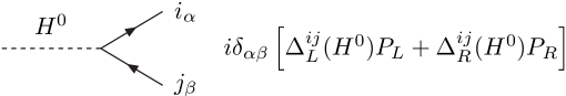
Figure 1: Feynman rules for a neutral colourless scalar particle $H^{0}$ with mass $M_{H}$, where $i,\,j$ denote different quark flavours and $\alpha,\,\beta$ the colours. $P_{L,R}=(1\mp\gamma_{5})/2$.

2.2 Scenarios for Scalar Couplings

In order to take these different possibilities into account and having also in mind that scalar couplings could be independent of quark masses, we consider the following four scenarios for their couplings to quarks keeping the pair $(i,j)$ fixed:

1. Left-handed Scenario (LHS) with complex $\Delta_{L}^{bq}\not=0$ and $\Delta_{R}^{bq}=0$,

2. Right-handed Scenario (RHS) with complex $\Delta_{R}^{bq}\not=0$ and $\Delta_{L}^{bq}=0$,

3. Left-Right symmetric Scenario (LRS) with complex $\Delta_{L}^{bq}=\Delta_{R}^{bq}\not=0$,

4. Left-Right asymmetric Scenario (ALRS) with complex $\Delta_{L}^{bq}=-\Delta_{R}^{bq}\not=0$,

with analogous scenarios for the pair $(s,d)$. For rare $B_{q}$ decays in which the ordering $qb$ is used, the rule (3) has to be applied to each scenario. For $K$ physics this is not required. In the course of our paper we will list specific examples of models that share the properties of these different scenarios. We will see that these simple cases will give us a profound insight into the flavour structure of models in which NP is dominated by left-handed scalar currents or right-handed scalar currents or left-handed and right-handed scalar currents of the same size. We will also consider a model in which both a scalar and a pseudoscalar with approximately the same mass couple equally to quarks and leptons. Moreover we will study a scenario with underlying flavour $U(2)^{3}$ symmetry which will imply relations between $\Delta_{L}^{bd}$ and $\Delta_{L}^{bs}$ couplings and interesting phenomenological consequences.

The idea of looking at NP scenarios with the dominance of certain quark couplings to neutral gauge bosons or neutral scalars is not new and has been motivated by detailed studies in concrete models like supersymmetric flavour models [3], LHT model with T-parity [4, 5] or Randall-Sundrum scenario with custodial protection (RSc) [6]. See also [7, 8]. Also our recent analysis of tree-level FCNCs mediated by $Z^{\prime}$ and $Z$ in [1] demonstrates this type of NP in a transparent manner.

2.3 Scalar vs Pseudoscalar

It will turn out to be useful to exhibit the differences between the scalar and pseudoscalar spin 0 particles, although one should emphasize that in the presence of CP violation, the mass eigenstate $H^{0}$ propagating in a tree-diagram is not necessarily a CP eigenstate. Therefore, generally the coupling to $\mu^{+}\mu^{-}$ appearing at many places in our paper can have the general structure

$$L=\frac{1}{2}\bar{\mu}(\Delta_{S}^{\mu\bar{\mu}}(H^{0})+\gamma_{5}\Delta_{P}^{\mu\bar{\mu}}(H^{0}))H\mu$$ (9)

where generalizing the Feynman rule in Fig. 1 to charged lepton couplings we have introduced:

$$\begin{split}&\Delta_{S}^{\mu\bar{\mu}}(H)=\Delta_{R}^{\mu\bar{\mu}}(H)+\Delta_{L}^{\mu\bar{\mu}}(H),\\ &\Delta_{P}^{\mu\bar{\mu}}(H)=\Delta_{R}^{\mu\bar{\mu}}(H)-\Delta_{L}^{\mu\bar{\mu}}(H).\end{split}$$ (10)

$\Delta^{\mu\bar{\mu}}_{S}$ is real and $\Delta^{\mu\bar{\mu}}_{P}$ purely imaginary as required by the hermiticity of the Hamiltonian which can be verified by means of (3).

The expressions for various observables will be first given in terms of the couplings $\Delta_{L,R}^{ij}(H)$ and $\Delta_{S,P}^{\mu\bar{\mu}}(H)$ and can be directly used in the case of the scalar particle being CP-even eigenstate, like $(H^{0},h)$ in 2HDM or MSSM setting $\Delta_{P}^{\mu\bar{\mu}}(H)=0$. However, when the mass eigenstate is a pseudoscalar $A$, implying $\Delta_{S}^{\mu\bar{\mu}}=0$, it will be useful to exhibit the i which we illustrate here for the $B_{s}^{0}$ system:

$$\Delta_{L}^{bs}(A)=-i\tilde{\Delta}_{L}^{bs}(A),\qquad\Delta_{R}^{bs}(A)=+i\tilde{\Delta}_{R}^{bs}(A),\qquad\Delta_{P}^{\mu\bar{\mu}}(A)=i\tilde{\Delta}_{P}^{\mu\bar{\mu}}(A).$$ (11)

Here the flavour violating couplings $\tilde{\Delta}_{L,R}^{bs}(A)$ are still complex, while $\tilde{\Delta}_{P}^{\mu\bar{\mu}}(A)$ is real.

The following useful relations follow from (3) and (11):

$$\Delta_{R}^{sb}(A)=i[\tilde{\Delta}^{bs}_{L}(A)]^{*},\qquad\Delta_{L}^{sb}(A)=-i[\tilde{\Delta}^{bs}_{R}(A)]^{*}.$$ (12)

As far as $\Delta F=2$ transitions are concerned this distinction between scalar and pseudoscalar mass eigenstate is only relevant in a concrete model in which the relevant couplings are given in terms of fundamental parameters. However, as in our numerical analysis we will treat the flavour violating quark-scalar couplings as arbitrary complex numbers to be bounded by $\Delta F=2$ observables it will not be possible to distinguish a scalar and pseudoscalar boson on the basis of $\Delta F=2$ transitions alone. On the other hand, when rare decays, in particular $B_{s,d}\to\mu^{+}\mu^{-}$, are considered there is a difference between these two cases as the pseudoscalar contributions interfere with SM contribution, while the scalar ones do not. Consequently the allowed values for $\tilde{\Delta}_{P}^{\mu\bar{\mu}}(A)$ and $\Delta_{S}^{\mu\bar{\mu}}(A)$ will differ from each other and we will find other differences. Finally, if both scalar and pseudoscalar contribute to tree-level decays and have approximately the same mass as well as couplings related by symmetries, also their contributions to $\Delta F=2$ processes differ. We will consider a simple example in the course of our presentation.

2.4 Steps

Let us then outline our strategy for the determination of flavour violating $H$ couplings to quarks and for finding correlations between flavour observables in the context of the simple scenarios listed above. Our strategy will only be fully effective in the second half of this decade, when hadronic uncertainties will be reduced and the data on various observables significantly improved. It involves ten steps including a number of working assumptions:

Step 1:

Determination of CKM parameters by means of tree-level decays and of the necessary non-perturbative parameters by means of lattice calculations. This step will provide the results for all observables considered below within the SM as well as all non-perturbative parameters entering the NP contributions. As $|V_{ub}|$ is presently poorly known, it will be interesting in the spirit of our recent papers [1, 9, 2] to investigate how the outcome of this step depends on the value of $|V_{ub}|$ with direct implications for the necessary size of NP contributions which will be different in different observables.

Step 2:

We will assume that the ratios

$$\frac{\Delta_{S,P}^{\mu\bar{\mu}}(H)}{M_{H}}$$ (13)

for scalar and pseudoscalar bosons have been determined in pure leptonic processes and that the scalar couplings to neutrinos are negligible. The properties of these couplings have been discussed above. In principle these ratios can be determined up to the sign from quark flavour violating processes and in fact we will be able to bound them from the present data on $B_{s}\to\mu^{+}\mu^{-}$ but their independent knowledge increases predictive power of our analysis. In particular the knowledge of their signs allows us to remove certain discrete ambiguities and is crucial for the distinction between LHS and RHS scenarios in $B_{s,d}\to\mu^{+}\mu^{-}$ decays. Of course, in concrete models like 2HDM or supersymmetric models these couplings depend on the fundamental parameters of a given model.

Step 3:

Here we will consider the $B_{s}^{0}$ system and the observables

$$\Delta M_{s},\quad S_{\psi\phi},\quad\mathcal{B}(B_{s}\to\mu^{+}\mu^{-}),\quad\mathcal{A}_{\Delta\Gamma}^{\mu^{+}\mu^{-}},\quad S^{s}_{\mu^{+}\mu^{-}},$$ (14)

where $\mathcal{A}_{\Delta\Gamma}^{\mu^{+}\mu^{-}}$ and $S^{s}_{\mu^{+}\mu^{-}}$ can be extracted from the time-dependent $B_{s}\to\mu^{+}\mu^{-}$ rate [10, 11]. Explicit expressions for these observables in terms of the relevant couplings can be found in Sections 3 and 4.

Concentrating in this step on the LHS scenario, NP contributions to these three observables are fully described by

$$\frac{\Delta_{L}^{bs}(H)}{M_{H}}=-\frac{\tilde{s}_{23}}{M_{H}}e^{-i\delta_{23}},\quad\frac{\Delta_{S,P}^{\mu\bar{\mu}}(H)}{M_{H}},$$ (15)

with the second ratio known from Step 2. Here $\tilde{s}_{23}\geq 0$ and it is found to be below unity but it does not represent any mixing parameter as in [12]. The minus sign is introduced to cancel the minus sign in $V_{ts}$ in the phenomenological formulae listed in the next section.

Thus we have five observables to our disposal and two parameters in the quark sector to determine. This allows to remove certain discrete ambiguities, determine all parameters uniquely for a given $M_{H}$ and predict correlations between these five observables that are characteristic for this scenario.

Step 4:

Repeating this exercise in the $B_{d}^{0}$ system we have to our disposal

$$\Delta M_{d},\quad S_{\psi K_{S}},\quad\mathcal{B}(B_{d}\to\mu^{+}\mu^{-}),\quad S^{d}_{\mu^{+}\mu^{-}}.$$ (16)

Explicit expressions for these observables in terms of the relevant couplings can be found in Sections 3 and 4.

Now NP contributions to these three observables are fully described by

$$\frac{\Delta_{L}^{bd}(H)}{M_{H}}=\frac{\tilde{s}_{13}}{M_{H}}e^{-i\delta_{13}},\quad\frac{\Delta_{S,P}^{\mu\bar{\mu}}(H)}{M_{H}},$$ (17)

with the last one known from Step 2 and bounded in Step 3. Again we can determine all the couplings uniquely for a given $M_{H}$. Our notations and sign conventions are as in Step 3 with $\tilde{s}_{13}\geq 0$ but no minus sign as $V_{td}$ has no such sign.

Step 5:

Moving to the $K$ system we have to our disposal

$$\varepsilon_{K},\quad K_{L}\to\pi^{0}\ell^{+}\ell^{-},\quad K_{L}\to\mu^{+}\mu^{-},$$ (18)

where in view of hadronic uncertainties the last decay on this list will only be used to make sure that the existing rough bound on its short distance branching ratio is satisfied. Unfortunately tree-level neutral Higgs contributions to $K^{+}\rightarrow\pi^{+}\nu\bar{\nu}$ and $K_{L}\rightarrow\pi^{0}\nu\bar{\nu}$ are expected to be negligible, but this fact by itself offers an important test and distinction from tree level neutral gauge boson exchanges where these decays could still be significantly affected [1]. Also the decays $K_{L}\to\pi^{0}\ell^{+}\ell^{-}$ are subject to considerable hadronic uncertainties and their measurements are not expected in this decade. Yet, as they are known to be sensitive to NP effects it is of interest to consider them as well and compare the scalar case with the case of $Z^{\prime}$ models [1].

In the present paper we do not study the ratio $\varepsilon^{\prime}/\varepsilon$, which is rather accurately measured but presently subject to much larger hadronic uncertainties than observables listed in (18). Yet, it should be emphasized that $\varepsilon^{\prime}/\varepsilon$ is important for the tests of $H$ FCNC scenarios as it is very sensitive to any NP contribution [13, 14, 15].

Explicit expressions for the observables in the $K$ system in terms of the relevant couplings can be found in Sections 3 and 5.

Now NP contributions to these observables are fully described by

$$\frac{\Delta_{L}^{sd}(H)}{M_{H}}=-\frac{\tilde{s}_{12}}{M_{H}}e^{-i\delta_{12}},\quad\frac{\Delta_{S,P}^{\mu\bar{\mu}}(H)}{M_{H}}$$ (19)

The ratios involving muon couplings are already constrained or determined in previous steps. Consequently, we can bound quark couplings involved by using the data on the observables in (18). Moreover we identify certain correlations characteristic for LHS scenario. $\tilde{s}_{12}\geq 0$ and the minus sign is chosen to cancel the one of $V_{ts}$.

We can already announce at this stage that the results in $K$ physics turned out to be much less interesting than in the $B_{s}$ and $B_{d}$ systems and we summarize them separately in Section 9.

Step 6:

As all parameters of LHS scenario have been fixed in the first five steps we are in the position to make predictions for the following processes

$$B\to X_{s}\ell^{+}\ell^{-},\quad B\to K\ell^{+}\ell^{-},\quad B\to K^{*}\ell^{+}\ell^{-}$$ (20)

and test whether they provide additional constraints on the couplings. Again as in the case of $K^{+}\rightarrow\pi^{+}\nu\bar{\nu}$ and $K_{L}\rightarrow\pi^{0}\nu\bar{\nu}$ also the $b\to s\nu\bar{\nu}$ transitions are expected to be SM-like which provides a distinction from the gauge boson mediated tree-level transitions [1].

Step 7:

We repeat Steps 3-6 for the case of RHS. We will see that in view of the change of the sign of NP contributions to $B_{s,d}\to\mu^{+}\mu^{-}$ and $K_{L}\to\mu^{+}\mu^{-}$ decays the structure of the correlations between various observables will distinguish this scenario from the LHS one. Yet, as we will find out, by going from LHS to RHS scenario we can keep results of Steps 3-5 unchanged by interchanging simultaneously two big oases in the parameter space that we encountered already in our study of the $\overline{331}$ model [12] and $Z^{\prime}$ models [1]. This LH-RH invariance present in Steps 3-5 can be broken by the $b\to s\ell^{+}\ell^{-}$ transition in (20). They allow us to distinguish the physics of RH scalar currents from LH ones. As only RH couplings are present in the NP contributions in this scenario, we can use the parametrization of these couplings as in (15), (17) and (19) keeping in mind that now RH couplings are involved.

Step 8:

We repeat Steps 3-6 for the case of LRS. In the case of tree-level gauge boson contributions the new features relative to the previous scenarios is enhanced NP contributions due to the presence of LR operators in $\Delta F=2$ transitions. Yet, in the scalar case, the matrix elements of SLL and SRR operators present in previous scenarios are also significant larger than the SM ones and the addition of LR operators has a more modest effect than in the gauge boson case. However, one of the important new feature is the vanishing of NP contributions to $B_{s,d}\to\mu^{+}\mu^{-}$ and $K_{L}\to\mu^{+}\mu^{-}$ decays. As the LH and RH couplings are equal we can again use the parametrization of these couplings as in (15), (17) and (19) but their values will change due to different constraints from $\Delta F=2$ transitions. Also in this step $b\to s\ell^{+}\ell^{-}$ transitions can play an important role.

Step 9:

We repeat Steps 3-6 for the case of ALRS. Here the new feature relatively to LRS are non-vanishing NP contributions to $B_{s,d}\to\mu^{+}\mu^{-}$, including $S^{d,s}_{\mu^{+}\mu^{-}}$ CP asymmetries. Again the $b\to s\ell^{+}\ell^{-}$ transitions will exhibit their strength in testing the theory in a different environment: NP contributions to $\Delta F=2$ observables due to the presence of LR operators. As the LH and RH couplings differ only by a sign we can again use the parametrization of these couplings as in (15), (17) and (19) but their values will change due to different constraints from $\Delta F=2$ transitions.

Step 10:

One can consider next the case of simultaneous LH and RH couplings that are unrelated to each other. This step is more challenging as one has more free parameters and in order to reach clear cut conclusions one would need a concrete model for $H$ couplings or a very involved numerical analysis [7, 8, 16]. A simple model in which both a scalar and a pseudoscalar with approximately the same mass couple equally to quarks and leptons has been recently presented in [17] showing that the structure of correlations can be quite rich. We refer to this paper for details.

Once this analysis of $H$ contributions is completed it will be straightforward to apply it to the case of the SM Higgs boson with flavour violating couplings. Yet, we will see that this case is less interesting than the case of $Z$ with flavour violating couplings.

3 $\Delta F=2$ Processes

3.1 Preliminaries

In the SM the dominant top quark contributions to $\Delta F=2$ processes are described by flavour universal real valued function given as follows ($x_{t}=m_{t}^{2}/M_{W}^{2}$):

$$S_{0}(x_{t})=\frac{4x_{t}-11x_{t}^{2}+x_{t}^{3}}{4(1-x_{t})^{2}}-\frac{3x_{t}^{2}\log x_{t}}{2(1-x_{t})^{3}}~{}.$$ (21)

In other CMFV models $S_{0}(x_{t})$ is replaced by a different function which is still flavour universal and is real valued. This implies very stringent relations between various observables in three meson system in question which have been reviewed in [18].

In the presence of $H$ tree-level contributions the flavour universality is generally broken and one needs three different functions

$$S(K),\qquad S(B_{d}),\qquad S(B_{s}),$$ (22)

to describe $K^{0}-\bar{K}^{0}$ and $B^{0}_{s,d}-\bar{B}^{0}_{s,d}$ systems. Moreover, they all become complex quantities. Therefore CMFV relations are generally broken. In introducing these functions we will include in their definitions the contributions of operators with $LL$, $RR$ and $LR$ Dirac structures.

The derivation of the formulae listed below is so simple that we will not present it here. In any case, the compendium of relevant formulae given below and in next sections is self-contained as far as numerical analysis is concerned.

3.2 Master Functions Including $H$ Contributions

Calculating the contributions of $H$ to $\Delta F=2$ transitions it is straightforward to write down the expressions for the master functions $S(M)$ in (22) in terms of the couplings defined in Fig. 1.

We define first the relevant CKM factors

$$\lambda_{i}^{(K)}=V_{is}^{*}V_{id},\qquad\lambda_{t}^{(d)}=V_{tb}^{*}V_{td},\qquad\lambda_{t}^{(s)}=V_{tb}^{*}V_{ts},$$ (23)

and introduce

$$g_{\text{SM}}^{2}=4\frac{G_{F}}{\sqrt{2}}\frac{\alpha}{2\pi\sin^{2}\theta_{W}}=1.78137\times 10^{-7}\,{\rm GeV}^{-2}\,.$$ (24)

The $\Delta F=2$ master functions for $M=K,B_{q}$ are then given as follows

$$S(M)=S_{0}(x_{t})+\Delta S(M)\equiv|S(M)|e^{i\theta_{S}^{M}}$$ (25)

with $\Delta S(M)$ receiving contributions from various operators so that it is useful to write

$$\Delta S(M)=[\Delta S(M)]_{\rm SLL}+[\Delta S(M)]_{\rm SRR}+[\Delta S(M)]_{\rm LR}.$$ (26)

The contributing new operators are defined for the $K$ system as follows [19, 20]

$${Q}_{1}^{\text{LR}} = \left(\bar{s}\gamma_{\mu}P_{L}d\right)\left(\bar{s}\gamma^{\mu}P_{R}d\right)\,,$$ (27a)

$${Q}_{2}^{\text{LR}} = \left(\bar{s}P_{L}d\right)\left(\bar{s}P_{R}d\right)\,.$$ (27b)

$${Q}_{1}^{\text{SLL}} = \left(\bar{s}P_{L}d\right)\left(\bar{s}P_{L}d\right)\,,$$ (28a)

$${Q}_{1}^{\text{SRR}} = \left(\bar{s}P_{R}d\right)\left(\bar{s}P_{R}d\right)\,,$$ (28b)

$${Q}_{2}^{\text{SLL}} = \left(\bar{s}\sigma_{\mu\nu}P_{L}d\right)\left(\bar{s}\sigma^{\mu\nu}P_{L}d\right)\,,$$ (28c)

$${Q}_{2}^{\text{SRR}} = \left(\bar{s}\sigma_{\mu\nu}P_{R}d\right)\left(\bar{s}\sigma^{\mu\nu}P_{R}d\right)\,,$$ (28d)

where $P_{R,L}=(1\pm\gamma_{5})/2$ and we suppressed colour indices as they are summed up in each factor. For instance $\bar{s}\gamma_{\mu}P_{L}d$ stands for $\bar{s}_{\alpha}\gamma_{\mu}P_{L}d_{\alpha}$ and similarly for other factors. For $B_{q}^{0}-\bar{B}_{q}^{0}$ mixing our conventions for new operators are:

$${Q}_{1}^{\text{LR}} = \left(\bar{b}\gamma_{\mu}P_{L}q\right)\left(\bar{b}\gamma^{\mu}P_{R}q\right)\,,$$ (29a)

$${Q}_{2}^{\text{LR}} = \left(\bar{b}P_{L}q\right)\left(\bar{b}P_{R}q\right)\,,$$ (29b)

$${Q}_{1}^{\text{SLL}} = \left(\bar{b}P_{L}q\right)\left(\bar{b}P_{L}q\right)\,,$$ (30a)

$${Q}_{1}^{\text{SRR}} = \left(\bar{b}P_{R}q\right)\left(\bar{b}P_{R}q\right)\,,$$ (30b)

$${Q}_{2}^{\text{SLL}} = \left(\bar{b}\sigma_{\mu\nu}P_{L}q\right)\left(\bar{b}\sigma^{\mu\nu}P_{L}q\right)\,,$$ (30c)

$${Q}_{2}^{\text{SRR}} = \left(\bar{b}\sigma_{\mu\nu}P_{R}q\right)\left(\bar{b}\sigma^{\mu\nu}P_{R}q\right)\,.$$ (30d)

In order to calculate the SLL, SRR and LR contributions to $\Delta S(M)$ we introduce quantities familiar from SM expressions for mixing amplitudes

$$T(B_{q})=\frac{G_{F}^{2}}{12\pi^{2}}F_{B_{q}}^{2}\hat{B}_{B_{q}}m_{B_{q}}M_{W}^{2}\left(\lambda_{t}^{(q)}\right)^{2}\eta_{B},$$ (31)

$$T(K)=\frac{G_{F}^{2}}{12\pi^{2}}F_{K}^{2}\hat{B}_{K}m_{K}M_{W}^{2}\left(\lambda_{t}^{(K)}\right)^{2}\eta_{2},$$ (32)

where $\eta_{i}$ are QCD corrections and $\hat{B}_{i}$ known SM non-perturbative factors.

Then

$$T(K)[\Delta S(K)]_{\rm SLL}=-\frac{(\Delta_{L}^{sd}(H))^{2}}{2M_{H}^{2}}\left[C_{1}^{\text{SLL}}(\mu_{H})\langle Q_{1}^{\text{SLL}}(\mu_{H},K)\rangle+C_{2}^{\text{SLL}}(\mu_{H})\langle Q_{2}^{\text{SLL}}(\mu_{H},K)\rangle\right]$$ (33)

with the SRR contribution obtained by replacing L by R. Note that this replacement only affects the coupling $\Delta_{L}^{sd}(H)$ as the hadronic matrix elements being evaluated in QCD remain unchanged and the Wilson coefficients have been so defined that they also remain unchanged. For LR contributions we find

$$T(K)[\Delta S(K)]_{\rm LR}=-\frac{\Delta_{L}^{sd}(H)\Delta_{R}^{sd}(H)}{M_{H}^{2}}\left[C_{1}^{\text{LR}}(\mu_{H})\langle Q_{1}^{\text{LR}}(\mu_{H},K)\rangle+C_{2}^{\text{LR}}(\mu_{H})\langle Q_{2}^{\text{LR}}(\mu_{H},K)\rangle\right]\,.$$ (34)

Including NLO QCD corrections [20] the Wilson coefficients of the involved operators are given by

$$C_{1}^{\text{SLL}}(\mu)=C_{1}^{\text{SRR}}(\mu) =1+\frac{\alpha_{s}}{4\pi}\left(-3\log\frac{M_{H}^{2}}{\mu^{2}}+\frac{9}{2}\right)\,,$$ (35)

$$\begin{split}C_{2}^{\text{SLL}}(\mu)=C_{2}^{\text{SRR}}(\mu)&=\frac{\alpha_{s}}{4\pi}\left(-\frac{1}{12}\log\frac{M_{H}^{2}}{\mu^{2}}+\frac{1}{8}\right)\,,\end{split}$$ (36)

$$C_{1}^{\text{LR}}(\mu) =-\frac{3}{2}\frac{\alpha_{s}}{4\pi}\,,$$ (37)

$$C_{2}^{\text{LR}}(\mu) =1-\frac{\alpha_{s}}{4\pi}\frac{3}{N}=1-\frac{\alpha_{s}}{4\pi}\,.$$ (38)

Next

$$\langle Q^{a}_{i}(\mu_{H},K)\rangle\equiv\frac{m_{K}F_{K}^{2}}{3}P^{a}_{i}(\mu_{H},K)$$ (39)

are the matrix elements of operators evaluated at the matching scale $\mu_{H}={\cal O}(M_{H})$ and $P^{a}_{i}$ are the coefficients introduced in [19]. The $\mu_{H}$ dependence of $P^{a}_{i}(\mu_{H})$ cancels the one of $\Delta_{L,R}(H)$ and of $C^{a}_{i}(\mu_{H})$ so that $S(K)$ does not depend on $\mu_{H}$. It should be emphasized at this point that in contrast to gauge boson couplings the couplings $\Delta_{L,R}(H)$ are scale dependent and consistently with the NLO calculation in [20] they are defined here at $\mu_{H}={\cal O}(M_{H})$. In our numerical calculations we will simply set $\mu_{H}=M_{H}$.

Similarly for $B_{q}$ systems we have

$$T(B_{q})[\Delta S(B_{q})]_{\rm SLL}=-\frac{(\Delta_{L}^{bq}(H))^{2}}{2M_{H}^{2}}\left[C_{1}^{\text{SLL}}(\mu_{H})\langle Q_{1}^{\text{SLL}}(\mu_{H},B_{q})\rangle+C_{2}^{\text{SLL}}(\mu_{H})\langle Q_{2}^{\text{SLL}}(\mu_{H},B_{q})\rangle\right]$$ (40)

$$T(B_{q})[\Delta S(B_{q})]_{\rm LR}=-\frac{\Delta_{L}^{bq}(H)\Delta_{R}^{bq}(H)}{M_{H}^{2}}\left[C_{1}^{\text{LR}}(\mu_{H})\langle Q_{1}^{\text{LR}}(\mu_{H},B_{q})\rangle+C_{2}^{\text{LR}}(\mu_{H})\langle Q_{2}^{\text{LR}}(\mu_{H},B_{q})\rangle\right]\,,$$ (41)

where the Wilson coefficients $C^{a}_{i}(\mu_{H})$ are as in the $K$ system and the matrix elements are given by

$$\langle Q^{a}_{i}(\mu_{H},B_{q})\rangle\equiv\frac{m_{B_{q}}F_{B_{q}}^{2}}{3}P^{a}_{i}(\mu_{H},B_{q}).$$ (42)

For SRR contributions one proceeds as in the $K$ system.

Finally, we collect in Table 1 central values of $\langle Q^{a}_{i}(\mu_{H})\rangle$. They are given in the $\overline{\text{MS}}$-NDR scheme and are based on lattice calculations in [21, 22] for $K^{0}-\bar{K}^{0}$ system and in [23] for $B_{d,s}^{0}-\bar{B}^{0}_{d,s}$ systems. For the $K^{0}-\bar{K}^{0}$ system we have just used the average of the results in [21, 22] that are consistent with each other. As the values of the relevant $B_{i}$ parameters in these papers have been evaluated at $\mu=3\,{\rm GeV}$ and $4.2\,{\rm GeV}$, respectively, we have used the formulae in [19] to obtain the values of the matrix elements in question at $\mu_{H}$. For simplicity we choose this scale to be $M_{H}$ but any scale of this order would give the same results for the physical quantities up to NNLO QCD corrections that are negligible at these high scales. The renormalization scheme dependence of the matrix elements is canceled by the one of the Wilson coefficients.

In the case of tree-level SM Higgs exchanges we evaluate the matrix elements at $m_{t}(m_{t})$ as the inclusion of NLO QCD corrections allows us to choose any scale of ${\cal O}(M_{H})$ without changing physical results. Then in the formulae above one should replace $M_{H}$ by the SM Higgs mass and $\mu_{H}$ by $m_{t}(m_{t})$. This also means that the flavour violating couplings of SM Higgs are defined here at $m_{t}(m_{t})$. The values of hadronic matrix elements at $m_{t}(m_{t})$ in the $\overline{\text{MS}}$-NDR scheme are given in Table 2.

	$\langle Q_{1}^{\text{LR}}(\mu_{H})\rangle$	$\langle Q_{2}^{\text{LR}}(\mu_{H})\rangle$	$\langle Q_{1}^{\text{SLL}}(\mu_{H})\rangle$	$\langle Q_{2}^{\text{SLL}}(\mu_{H})\rangle$
$K^{0}$-$\bar{K}^{0}$	$-0.14$	$0.22$	$-0.074$	$-0.128$
$B_{d}^{0}$-$\bar{B}_{d}^{0}$	$-0.25$	$0.34$	$-0.11$	$-0.22$
$B_{s}^{0}$-$\bar{B}_{s}^{0}$	$-0.37$	$0.51$	$-0.17$	$-0.33$

Table 1: Hadronic matrix elements $\langle Q_{i}^{a}(\mu_{H})\rangle$ in units of GeV³ at $\mu_{H}=1\,{\rm TeV}$.

	$\langle Q_{1}^{\text{LR}}(m_{t})\rangle$	$\langle Q_{2}^{\text{LR}}(m_{t})\rangle$	$\langle Q_{1}^{\text{SLL}}(m_{t})\rangle$	$\langle Q_{2}^{\text{SLL}}(m_{t})\rangle$
$K^{0}$-$\bar{K}^{0}$	$-0.11$	$0.18$	$-0.064$	$-0.107$
$B_{d}^{0}$-$\bar{B}_{d}^{0}$	$-0.21$	$0.27$	$-0.095$	$-0.191$
$B_{s}^{0}$-$\bar{B}_{s}^{0}$	$-0.30$	$0.40$	$-0.14$	$-0.29$

Table 2: Hadronic matrix elements $\langle Q_{i}^{a}(\mu_{t})\rangle$ in units of GeV³ at $m_{t}(m_{t})$.

3.3 Basic Formulae for $\Delta F=2$ Observables

The $\Delta B=2$ mass differences are given as follows:

$$\Delta M_{d}=\frac{G_{F}^{2}}{6\pi^{2}}M_{W}^{2}m_{B_{d}}|\lambda_{t}^{(d)}|^{2}F_{B_{d}}^{2}\hat{B}_{B_{d}}\eta_{B}|S(B_{d})|\,,$$ (43)

$$\Delta M_{s}=\frac{G_{F}^{2}}{6\pi^{2}}M_{W}^{2}m_{B_{s}}|\lambda_{t}^{(s)}|^{2}F_{B_{s}}^{2}\hat{B}_{B_{s}}\eta_{B}|S(B_{s})|\,.$$ (44)

The corresponding mixing induced CP-asymmetries are then given by

$$S_{\psi K_{S}}=\sin(2\beta+2\varphi_{B_{d}})\,,\qquad S_{\psi\phi}=\sin(2|\beta_{s}|-2\varphi_{B_{s}})\,,$$ (45)

where the phases $\beta$ and $\beta_{s}$ are defined by

$$V_{td}=|V_{td}|e^{-i\beta},\qquad V_{ts}=-|V_{ts}|e^{-i\beta_{s}}.$$ (46)

$\beta_{s}\simeq-1^{\circ}\,$. The new phases $\varphi_{B_{q}}$ are directly related to the phases of the functions $S(B_{q})$:

$$2\varphi_{B_{q}}=-\theta_{S}^{B_{q}}.$$ (47)

Our phase conventions are as in [1] and our previous papers quoted in this work. Consequently $S_{\psi\phi}^{\rm SM}\approx 0.04$. On the other hand the experimental results are usually given for the phase

$$\phi_{s}=2\beta_{s}+\phi^{\rm NP}$$ (48)

so that

$$S_{\psi\phi}=-\sin(\phi_{s}),\qquad 2\varphi_{B_{s}}=\phi^{\rm NP}.$$ (49)

Using this dictionary the most recent result for $\phi_{s}$ from the LHCb analysis of CP-violation in $B_{s}\to\psi\phi$ decay implies [24]

$$2|\beta_{s}|-2\varphi_{B_{s}}=0.001\pm 0.104,$$ (50)

that is close to its SM value. But the uncertainties are still sufficiently large so that it is of interest to investigate correlations of $S_{\psi\phi}$ with other observables in the $B_{s}$ system.

For the CP-violating parameter $\varepsilon_{K}$ and $\Delta M_{K}$ we have respectively

$$\varepsilon_{K}=\frac{\kappa_{\varepsilon}e^{i\varphi_{\varepsilon}}}{\sqrt{2}(\Delta M_{K})_{\text{exp}}}\left[\Im\left(M_{12}^{K}\right)\right]\,,\qquad\Delta M_{K}=2\Re\left(M_{12}^{K}\right),$$ (51)

where

$$\left(M_{12}^{K}\right)^{*}=\frac{G_{F}^{2}}{12\pi^{2}}F_{K}^{2}\hat{B}_{K}m_{K}M_{W}^{2}\left[\lambda_{c}^{2}\eta_{1}x_{c}+\lambda_{t}^{2}\eta_{2}S(K)+2\lambda_{c}\lambda_{t}\eta_{3}S_{0}(x_{c},x_{t})\right]\,.$$ (52)

Here, $S_{0}(x_{c},x_{t})$ is a real valued one-loop box function for which explicit expression is given e. g. in [25]. The factors $\eta_{i}$ are QCD corrections evaluated at the NLO level in [26, 27, 28, 29, 30]. For $\eta_{1}$ and $\eta_{3}$ also NNLO corrections are known [31, 32]. Next $\varphi_{\varepsilon}=(43.51\pm 0.05)^{\circ}$ and $\kappa_{\varepsilon}=0.94\pm 0.02$ [33, 34] takes into account that $\varphi_{\varepsilon}\neq\tfrac{\pi}{4}$ and includes long distance effects in $\Im(\Gamma_{12})$ and $\Im(M_{12})$.

In the rest of the paper, unless otherwise stated, we will assume that all four parameters in the CKM matrix have been determined through tree-level decays without any NP pollution and pollution from QCD-penguin diagrams so that their values can be used universally in all NP models considered by us.

4 Rare B Decays

4.1 Preliminaries

These decays played already for many years a significant role in constraining NP models. In particular $B_{s}\to\mu^{+}\mu^{-}$ was instrumental in bounding scalar contributions in the framework of supersymmetric models and two Higgs doublet models (2HDM). Recently a very detailed analysis of the decay $B_{s}\to\mu^{+}\mu^{-}$ including the observables involved in the time-dependent rate has been presented [17]. Below, after recalling the relevant effective Hamiltonian that can be used for other $b\to s\ell^{+}\ell^{-}$ transitions, we will summarize the final formulae for the most important observables in $B_{s}\to\mu^{+}\mu^{-}$ that have been derived and discussed in more detail in [17] and in particular earlier in [11]. While our analysis of $B_{s}\to\mu^{+}\mu^{-}$ is less detailed than the one in [17], our main goal here is to discuss the correlations of $B_{s}\to\mu^{+}\mu^{-}$ observables with $\Delta F=2$ observables, in particular $S_{\psi\phi}$, which were not presented there. Moreover, we analyze here similar correlations involving $B_{d}\to\mu^{+}\mu^{-}$ observables and $S_{\psi K_{S}}$.

4.2 Effective Hamiltonian for $b\to s\ell^{+}\ell^{-}$

For our discussion of $B_{d,s}\to\mu^{+}\mu^{-}$ and for the imposition of the constraints from other $b\to s\ell^{+}\ell^{-}$ transitions, like $B\to K^{*}\ell^{+}\ell^{-}$, $B\to K\ell^{+}\ell^{-}$ and $B\to X_{s}\ell^{+}\ell^{-}$, we will need the corresponding effective Hamiltonian which is a generalization of the SM one:

$${\cal H}_{\text{ eff}}(b\to s\ell\bar{\ell})={\cal H}_{\text{ eff}}(b\to s\gamma)-\frac{4G_{\rm F}}{\sqrt{2}}\frac{\alpha}{4\pi}V_{ts}^{*}V_{tb}\sum_{i=9,10,S,P}[C_{i}(\mu)Q_{i}(\mu)+C^{\prime}_{i}(\mu)Q^{\prime}_{i}(\mu)]$$ (53)

where

$$Q_{9} =(\bar{s}\gamma_{\mu}P_{L}b)(\bar{\ell}\gamma^{\mu}\ell), Q_{9}^{\prime}=(\bar{s}\gamma_{\mu}P_{R}b)(\bar{\ell}\gamma^{\mu}\ell),$$ (54a)

$$Q_{10} =(\bar{s}\gamma_{\mu}P_{L}b)(\bar{\ell}\gamma^{\mu}\gamma_{5}\ell), Q_{10}^{\prime}=(\bar{s}\gamma_{\mu}P_{R}b)(\bar{\ell}\gamma^{\mu}\gamma_{5}\ell),$$ (54b)

$$Q_{S} =m_{b}(\bar{s}P_{R}b)(\bar{\ell}\ell), Q_{S}^{\prime}=m_{b}(\bar{s}P_{L}b)(\bar{\ell}\ell),$$ (54c)

$$Q_{P} =m_{b}(\bar{s}P_{R}b)(\bar{\ell}\gamma_{5}\ell), Q_{P}^{\prime}=m_{b}(\bar{s}P_{L}b)(\bar{\ell}\gamma_{5}\ell).$$ (54d)

Including the factors of $m_{b}$ into the definition of scalar operators makes their matrix elements and their Wilson coefficients scale independent. ${\cal H}_{\text{ eff}}(b\to s\gamma)$ stands for the effective Hamiltonian for the $b\to s\gamma$ transition that involves the dipole operators. We will not discuss $b\to s\gamma$ in this paper as it appears first at one-loop level and a neutral scalar contribution would only be of relevance in the presence of flavor-conserving scalar couplings to down-type quarks which would introduce new parameters without any impact on our results.

Note the difference of ordering of flavours relatively to $\Delta F=2$ as already stressed in Section 2. Therefore the unprimed operators $Q_{S}$ and $Q_{P}$ represent the LHS scenario and the primed ones $Q_{S}^{\prime}$ and $Q_{P}^{\prime}$ the RHS scenario. We neglect effects proportional to $m_{s}$ in each case but keep $m_{s}$ and $m_{d}$ different from zero when they are shown explicitly.

The Wilson coefficients $C_{9}$ and $C_{10}$ do not receive any new contributions from scalar exchanges and take SM values

$$\sin^{2}\theta_{W}C^{\rm SM}_{9} =[\eta_{Y}Y_{0}(x_{t})-4\sin^{2}\theta_{W}Z_{0}(x_{t})],$$ (55)

$$\sin^{2}\theta_{W}C^{\rm SM}_{10} =-\eta_{Y}Y_{0}(x_{t}).$$ (56)

On the other hand with $m_{s}\ll m_{b}$ we have $C_{9}^{\prime}=C_{10}^{\prime}=0$. Here $Y_{0}(x_{t})$ and $Z_{0}(x_{t})$ are SM one-loop functions given by

$$Y_{0}(x_{t})=\frac{x_{t}}{8}\left(\frac{x_{t}-4}{x_{t}-1}+\frac{3x_{t}\log x_{t}}{(x_{t}-1)^{2}}\right),$$ (57)

$$Z_{0}(x) =-\frac{1}{9}\log x+\frac{18x^{4}-163x^{3}+259x^{2}-108x}{144(x-1)^{3}}+\frac{32x^{4}-38x^{3}-15x^{2}+18x}{72(x-1)^{4}}\log x\,.$$ (58)

The coefficient $\eta_{Y}$ is a QCD factor which for $m_{t}=m_{t}(m_{t})$ is close to unity: $\eta_{Y}=1.012$ [35, 36].

For the coefficients of scalar operators we find

$$m_{b}(\mu_{H})\sin^{2}\theta_{W}C_{S} =\frac{1}{g_{\text{SM}}^{2}}\frac{1}{M_{H}^{2}}\frac{\Delta_{R}^{sb}(H)\Delta_{S}^{\mu\bar{\mu}}(H)}{V_{ts}^{*}V_{tb}},$$ (59)

$$m_{b}(\mu_{H})\sin^{2}\theta_{W}C_{S}^{\prime} =\frac{1}{g_{\text{SM}}^{2}}\frac{1}{M_{H}^{2}}\frac{\Delta_{L}^{sb}(H)\Delta_{S}^{\mu\bar{\mu}}(H)}{V_{ts}^{*}V_{tb}},$$ (60)

$$m_{b}(\mu_{H})\sin^{2}\theta_{W}C_{P} =\frac{1}{g_{\text{SM}}^{2}}\frac{1}{M_{H}^{2}}\frac{\Delta_{R}^{sb}(H)\Delta_{P}^{\mu\bar{\mu}}(H)}{V_{ts}^{*}V_{tb}},$$ (61)

$$m_{b}(\mu_{H})\sin^{2}\theta_{W}C_{P}^{\prime} =\frac{1}{g_{\text{SM}}^{2}}\frac{1}{M_{H}^{2}}\frac{\Delta_{L}^{sb}(H)\Delta_{P}^{\mu\bar{\mu}}(H)}{V_{ts}^{*}V_{tb}},$$ (62)

where $\Delta_{S,P}^{\mu\bar{\mu}}(H)$ are defined in (LABEL:equ:mumuSPLR). It should be emphasized at this point that the couplings $\Delta_{L,R}^{sb}(H)$ extracted from $\Delta M_{s}$ and $S_{\psi\phi}$ are defined at $\mu_{H}=M_{H}$, therefore, as shown explicitly, $m_{b}$ has to be evaluated also at this scale in order to keep these coefficients scale independent. In the case of the SM Higgs $m_{b}$ has to be evaluated at $m_{t}(m_{t})$ as at this scale the flavour violating SM Higgs couplings in $\Delta F=2$ processes are defined. In what follows we will not show this dependence explicitly. For $m_{b}$ at $1~{}$TeV and at $125~{}$GeV we use the values

$$m_{b}(1~{}\text{TeV})=2.54~{}\text{GeV}\,,\qquad m_{b}(163~{}\text{GeV})=2.81~{}\text{GeV}\,.$$ (63)

Next we recall that in terms of the couplings used in the analysis of $B_{s,d}^{0}-\bar{B}_{s,d}^{0}$ mixings we have

$$\Delta_{R}^{sb}(H)=[\Delta_{L}^{bs}(H)]^{*},\qquad\Delta_{L}^{sb}(H)=[\Delta_{R}^{bs}(H)]^{*},$$ (64)

which should be kept in mind when studying correlations between $\Delta F=1$ and $\Delta F=2$ transitions. These relations can be directly used in the case of $C_{S}$ and $C_{S}^{\prime}$ but in the case of $C_{P}$ and $C_{P}^{\prime}$, as discussed in Section 2, it is useful to use in this context the following relations:

$$\Delta_{R}^{sb}\Delta_{P}^{\mu\bar{\mu}}=-[\tilde{\Delta}_{L}^{bs}]^{*}\tilde{\Delta}_{P}^{\mu\bar{\mu}},\qquad\Delta_{L}^{sb}\Delta_{P}^{\mu\bar{\mu}}=[\tilde{\Delta}_{R}^{bs}]^{*}\tilde{\Delta}_{P}^{\mu\bar{\mu}}$$ (65)

with $\Delta_{P}^{\mu\bar{\mu}}$ being imaginary but $\tilde{\Delta}_{P}^{\mu\bar{\mu}}$ real.

4.3 Observables for $B_{s}\to\mu^{+}\mu^{-}$

In the general analysis of $B_{s}\to\mu^{+}\mu^{-}$ in [17], which goes beyond the NP scenario considered here, the basic four observables are

$$\overline{R},\qquad\mathcal{A}^{\mu\mu}_{\Delta\Gamma},\qquad S^{s}_{\mu\mu},\quad S_{\psi\phi}.$$ (66)

Here, the observable $\overline{R}$, defined in (4.3), is just the ratio of the branching ratio that includes $\Delta\Gamma_{s}$ effects and of the SM prediction for the branching ratio that also includes them. The relation of $\overline{R}$ to $R$ introduced in [11] is given below. Following [17] we will denote branching ratios containing $\Delta\Gamma_{s}$ effects with a bar while those without these effects without it.

The next two observables, ${\cal A}^{\mu\mu}_{\Delta\Gamma}$ and ${\cal S}_{\mu\mu}$ can be extracted from flavour untagged and tagged time-dependent measurements of $B_{s}\to\mu^{+}\mu^{-}$, respectively. As these three observables depend also on the new phase $\varphi_{B_{s}}$ in the $B_{s}^{0}-\bar{B}_{s}^{0}$ mixing, also the mixing induced CP-asymmetry $S_{\psi\phi}$ is involved here.

In order to calculate these observables one introduces

$$P \equiv\frac{C_{10}-C_{10}^{\prime}}{C_{10}^{\rm SM}}+\frac{m^{2}_{B_{s}}}{2m_{\mu}}\frac{m_{b}}{m_{b}+m_{s}}\frac{C_{P}-C_{P}^{\prime}}{C_{10}^{\rm SM}}\equiv|P|e^{i\varphi_{P}}$$ (67)

$$S \equiv\sqrt{1-\frac{4m_{\mu}^{2}}{m_{B_{s}}^{2}}}\frac{m^{2}_{B_{s}}}{2m_{\mu}}\frac{m_{b}}{m_{b}+m_{s}}\frac{C_{S}-C_{S}^{\prime}}{C_{10}^{\rm SM}}\equiv|S|e^{i\varphi_{S}}.$$ (68)

One finds then three basic formulae [11, 37, 17]

$$\overline{R} \equiv\frac{\overline{\mathcal{B}}(B_{s}\to\mu^{+}\mu^{-})}{\overline{\mathcal{B}}(B_{s}\to\mu^{+}\mu^{-})_{\rm SM}}=\left[\frac{1+{\cal A}^{\mu\mu}_{\Delta\Gamma}\,y_{s}}{1+y_{s}}\right]\times(|P|^{2}+|S|^{2})$$

$$=\left[\frac{1+y_{s}\cos(2\varphi_{P}-2\varphi_{B_{s}})}{1+y_{s}}\right]|P|^{2}+\left[\frac{1-y_{s}\cos(2\varphi_{S}-2\varphi_{B_{s}})}{1+y_{s}}\right]|S|^{2},$$ (69)

$${\cal A}^{\mu\mu}_{\Delta\Gamma} =\frac{|P|^{2}\cos(2\varphi_{P}-2\varphi_{B_{s}})-|S|^{2}\cos(2\varphi_{S}-2\varphi_{B_{s}})}{|P|^{2}+|S|^{2}},$$ (70)

$$S^{s}_{\mu\mu} =\frac{|P|^{2}\sin(2\varphi_{P}-2\varphi_{B_{s}})-|S|^{2}\sin(2\varphi_{S}-2\varphi_{B_{s}})}{|P|^{2}+|S|^{2}}.$$ (71)

Here [38]

$$y_{s}\equiv\tau_{B_{s}}\frac{\Delta\Gamma_{s}}{2}=0.088\pm 0.014.$$ (72)

The ratio $R$ of [11], which did not include $\Delta\Gamma_{s}$ effects in the SM result and $\overline{R}$ which includes them are related by

$$\overline{R}=(1-y_{s})R.$$ (73)

The advantage of $\overline{R}$ over $R$ is that in the SM it is equal to unity and its departure from unity summarizes total NP effects present both in the decay and mixing.

Another useful variable encountered in this discussion is

$$r(y_{s})\equiv\frac{1-y_{s}^{2}}{1+\mathcal{A}^{\mu^{+}\mu^{-}}_{\Delta\Gamma}y_{s}}.$$ (74)

It is the correction factor that one has to introduce in any model in order to compare the branching ratio calculated in this model without $\Delta\Gamma_{s}$ effects and the branching ratio which includes them [39, 10, 11]

$$\mathcal{B}(B_{s}\to\mu^{+}\mu^{-})=r(y_{s})~{}\overline{\mathcal{B}}(B_{s}\to\mu^{+}\mu^{-}).$$ (75)

It should be emphasized that presently only $\overline{\mathcal{B}}(B_{s}\to\mu^{+}\mu^{-})$ is known experimentally but once $\mathcal{A}^{\mu\mu}_{\Delta\Gamma}$ will be extracted from time-dependent measurements, we will be able to obtain $\mathcal{B}(B_{s}\to\mu^{+}\mu^{-})$ directly from experiment as well. Evidently, in any model the branching ratios without $\Delta\Gamma_{s}$ effect are related to the corresponding SM branching ratio through

$$\mathcal{B}(B_{s}\to\mu^{+}\mu^{-})=\mathcal{B}(B_{s}\to\mu^{+}\mu^{-})_{\rm SM}(|P|^{2}+|S|^{2}).$$ (76)

As $F_{B_{s}}$ cancels out in the evaluation of $\mathcal{A}^{\mu\mu}_{\Delta\Gamma}$ and ${\cal S}_{\mu\mu}$, these are theoretically clean observables and offer new ways to test NP models. Indeed, as seen in (70) and (71), both observables depend on NP contributions and this is also the case of the conversion factor $r(y_{s})$. In the SM and CMFV models $S=0$ and $\varphi_{P}=\varphi_{B_{s}}=0$ so that

$$\mathcal{A}^{\mu\mu}_{\Delta\Gamma}=1,\quad S_{\mu\mu}^{s}=0,\quad r(y_{s})=0.912\pm 0.014\qquad({\rm SM,~{}CMFV}),$$ (77)

independently of NP parameters present in the whole class of CMFV models.

As $\mathcal{A}^{\mu\mu}_{\Delta\Gamma}$ does not rely on flavour tagging, which is difficult for a rare decay, it will be easier to determine than $S_{\mu\mu}^{s}$. Given limited statistics, experiments may first measure the $B_{s}\to\mu^{+}\mu^{-}$ effective lifetime, a single exponential fit to the untagged rate, from which $\mathcal{A}^{\mu\mu}_{\Delta\Gamma}$ can also be deduced [11]. See also [17] for discussion.

While $\Delta\Gamma_{d}$ is very small and $y_{d}$ can be set to zero, in the case of $B_{d}\to\mu^{+}\mu^{-}$ one can still consider the CP asymmetry $S_{\mu\mu}^{d}$ [37], for which one can use all expressions given above with the flavour index “$s$” replaced by “$d$”.

4.4 Present Data

The most recent results from LHCb read [40, 41]

$$\overline{\mathcal{B}}(B_{s}\to\mu^{+}\mu^{-})=(3.2^{+1.5}_{-1.2})\times 10^{-9},\quad\mathcal{B}(B_{s}\to\mu^{+}\mu^{-})_{\rm SM}=(3.25\pm 0.17)\times 10^{-9},$$ (78)

$$\mathcal{B}(B_{d}\to\mu^{+}\mu^{-})\leq 9.4\times 10^{-10},\quad\mathcal{B}(B_{d}\to\mu^{+}\mu^{-})_{\rm SM}=(1.05\pm 0.07)\times 10^{-10}.$$ (79)

We have shown here SM predictions for these observables that do not include the correction ${r(y_{s})}$. As $r(y_{d})=1$ to an excellent approximation, the result for $B_{d}\to\mu^{+}\mu^{-}$ can be directly compared with experiment. In order to obtain these results we have used the parametric formulae of [42] and updated the lattice QCD values of $F_{B_{s,d}}$ [43] and the life-times $\tau_{B_{s,d}}$ [44]. Details can be found in [17].

If the correction factor ${r(y_{s})}$ is taken into account the SM result in (78) changes to [17]

$$\overline{\mathcal{B}}(B_{s}\to\mu^{+}\mu^{-})_{\rm SM}=(3.56\pm 0.18)\cdot 10^{-9}.$$ (80)

It is this branching that should be compared in such a case with the results of LHCb given above. For the latest discussions of these issues see [10, 11, 42, 37]. As discussed in [42, 45] complete NLO electroweak corrections are still missing in this estimate. This result should be available in the near future.

In our numerical results we will use $\overline{\mathcal{B}}(B_{s}\to\mu^{+}\mu^{-})$ in (75) with $\mathcal{B}(B_{s}\to\mu^{+}\mu^{-})$ given by (76) and $r(y_{s})$ by (74) with $\mathcal{A}^{\mu\mu}_{\Delta\Gamma}$ also affected by NP effects.

Combining the experimental and theoretical results quoted above gives

$$\overline{R}_{\rm LHCb}=0.90^{+0.42}_{-0.34}\in[0.30,1.80]\,(95\%\ {\rm C.L}).$$ (81)

This range should be compared with its SM value, corresponding to $P=1$, $S=0$ and $\phi_{s}^{\rm NP}=0$:

$$\overline{R}_{\rm SM}=1.$$ (82)

4.5 Scenarios for $S$ and $P$

Clearly, the outcome of the results for the observables in question depends on the values of the muon couplings and whether a scalar or pseudoscalar boson is involved. Moreover, as we stressed already in Section 2 the exchanged mass eigenstate does not have to be a CP eigenstate and can have both scalar and pseudoscalar couplings to leptons. In [17] a detailed classification of various possibilities beyond the dynamical model considered here has been made and the related purely phenomenological numerical analysis has been performed. Here we will make a classification that is particularly suited for the dynamical model considered by us.

Pseudoscalar Scenario:

In this scenario $S=0$ and $P$ can be arbitrary complex number. We find then

$${\cal A}^{\mu\mu}_{\Delta\Gamma}=\cos(2\varphi_{P}-2\varphi_{B_{s}}),\quad S^{s}_{\mu\mu}=\sin(2\varphi_{P}-2\varphi_{B_{s}}).$$ (83)

The branching ratio observable is given by

$$\overline{R}=|P|^{2}\left[\frac{1+y_{s}\cos(2\varphi_{P}-2\varphi_{B_{s}})}{1+y_{s}}\right].$$ (84)

This scenario corresponds to scenario A in [17].

Scalar Scenario:

In this scenario $P=1$ and $S$ can be arbitrary complex number. We find then

$${\cal A}^{\mu\mu}_{\Delta\Gamma} =\frac{\cos 2\varphi_{B_{s}}-|S|^{2}\cos(2\varphi_{S}-2\varphi_{B_{s}})}{1+|S|^{2}},$$

$$S^{s}_{\mu\mu} =\frac{-\sin 2\varphi_{B_{s}}-|S|^{2}\sin(2\varphi_{S}-2\varphi_{B_{s}})}{1+|S|^{2}},$$

$$\overline{R} =\frac{1+y_{s}\cos 2\varphi_{B_{s}}}{1+y_{s}}+|S|^{2}\left[\frac{1-y_{s}\cos(2\varphi_{S}-2\varphi_{B_{s}})}{1+y_{s}}\right].$$ (85)

This scenario corresponds to scenario B in [17].

Mixed Scenario:

We will consider a scenarios in which $P$ is modified from its SM value and $S$ is non-zero. As we want to discuss the case of a single new particle with spin 0, this means that this particle has both scalar and pseudoscalar couplings to muons.

A simple scenario with both a scalar ($H^{0}$) and pseudoscalar ($A^{0}$) with approximately the same mass that couple equally to quarks and leptons up to the usual i factor in the pseudoscalar coupling has been recently considered in [17]. This scenario can be realized as a special limit in models like 2HDM and the MSSM with interesting consequences for $\mathcal{A}^{\mu\mu}_{\Delta\Gamma}$. We refer to [17] for details.

5 Rare $K$ Decays

5.1 Effective Hamiltonian for $d\to s\ell^{+}\ell^{-}$

For the study of $K_{L}\to\mu^{+}\mu^{-}$ and $K_{L}\to\pi^{0}\ell⁺\ell^{-}$ decays we will need the relevant effective Hamiltonian. It can be obtained from the formulae of subsection 4.2. For completeness we list here explicit formulae for operators and Wilson coefficients:

$$Q_{9} =(\bar{s}\gamma_{\mu}P_{L}d)(\bar{\ell}\gamma^{\mu}\ell), Q_{9}^{\prime}=(\bar{s}\gamma_{\mu}P_{R}d)(\bar{\ell}\gamma^{\mu}\ell),$$ (86a)

$$Q_{10} =(\bar{s}\gamma_{\mu}P_{L}d)(\bar{\ell}\gamma^{\mu}\gamma_{5}\ell), Q_{10}^{\prime}=(\bar{s}\gamma_{\mu}P_{R}d)(\bar{\ell}\gamma^{\mu}\gamma_{5}\ell),$$ (86b)

$$Q_{S} =m_{s}(\bar{s}P_{L}d)(\bar{\ell}\ell), Q_{S}^{\prime}=m_{s}(\bar{s}P_{R}d)(\bar{\ell}\ell),$$ (86c)

$$Q_{P} =m_{s}(\bar{s}P_{L}d)(\bar{\ell}\gamma_{5}\ell), Q_{P}^{\prime}=m_{s}(\bar{s}P_{R}d)(\bar{\ell}\gamma_{5}\ell).$$ (86d)

Note that because of the $sd$ ordering instead of $qb$ scalar operators have $L$ and $R$ interchanged with respect to $b\to s,d$ transitions.

The Wilson coefficients $C_{9}$ and $C_{10}$ do not receive any new contributions from scalar exchange and take SM values as given in (55). However, in order to include charm component in $K_{L}\to\mu^{+}\mu^{-}$ we make replacement:

$$\eta_{Y}Y_{0}(x_{t})\longrightarrow\eta_{Y}Y_{0}(x_{t})+\frac{V_{cs}^{*}V_{cd}}{V_{ts}^{*}V_{td}}Y_{\rm NNL}$$ (87)

where at NNLO [46]

$$Y_{\rm NNL}=\lambda^{4}P_{c}(Y),\qquad P_{c}(Y)=0.113\pm 0.017~{}.$$ (88)

The coefficients of scalar operators are:

$$m_{s}\sin^{2}\theta_{W}C_{S} =\frac{1}{g_{\text{SM}}^{2}}\frac{1}{M_{H}^{2}}\frac{\Delta_{L}^{sd}(H)\Delta_{S}^{\mu\bar{\mu}}(H)}{V_{ts}^{*}V_{td}},$$ (89)

$$m_{s}\sin^{2}\theta_{W}C_{S}^{\prime} =\frac{1}{g_{\text{SM}}^{2}}\frac{1}{M_{H}^{2}}\frac{\Delta_{R}^{sd}(H)\Delta_{S}^{\mu\bar{\mu}}(H)}{V_{ts}^{*}V_{td}},$$ (90)

$$m_{s}\sin^{2}\theta_{W}C_{P} =\frac{1}{g_{\text{SM}}^{2}}\frac{1}{M_{H}^{2}}\frac{\Delta_{L}^{sd}(H)\Delta_{P}^{\mu\bar{\mu}}(H)}{V_{ts}^{*}V_{td}},$$ (91)

$$m_{s}\sin^{2}\theta_{W}C_{P}^{\prime} =\frac{1}{g_{\text{SM}}^{2}}\frac{1}{M_{H}^{2}}\frac{\Delta_{R}^{sd}(H)\Delta_{P}^{\mu\bar{\mu}}(H)}{V_{ts}^{*}V_{td}}.$$ (92)

5.2 $K_{L}\to\mu^{+}\mu^{-}$

Only the so-called short distance (SD) part to a dispersive contribution to $K_{L}\to\mu^{+}\mu^{-}$ can be reliably calculated. Therefore in what follows this decay will be treated only as an additional constraint to be sure that the rough upper bound given below is not violated.

The relevant branching ratio can be obtained by first introducing:

$$\hat{P}(K)\equiv{C_{10}-C_{10}^{\prime}}+\frac{m^{2}_{K}}{2m_{\mu}}\frac{m_{s}}{m_{d}+m_{s}}(C_{P}-C_{P}^{\prime})$$ (93)

$$\hat{S}(K)\equiv\sqrt{1-\frac{4m_{\mu}^{2}}{m_{K}^{2}}}\frac{m^{2}_{K}}{2m_{\mu}}\frac{m_{s}}{m_{d}+m_{s}}(C_{S}-C_{S}^{\prime})$$ (94)

We then find

$$\mathcal{B}(K_{L}\to\mu^{+}\mu^{-})_{\rm SD}= \frac{G_{F}^{4}M_{W}^{4}}{4\pi^{5}}F_{K}^{2}m_{K}\tau_{K_{L}}m_{\mu}^{2}\sqrt{1-\frac{4m_{\mu}^{2}}{m_{K}^{2}}}\sin^{4}\theta_{W}$$ (95)

$$\times\left\{\left[\Re\left(V_{ts}^{*}V_{td}\hat{P}\right)\right]^{2}+\left[\Im\left(V_{ts}^{*}V_{td}\hat{S}\right)\right]^{2}\right\}$$

and $\Re\leftrightarrow\Im$ for $K_{S}\to\mu^{+}\mu^{-}$ decay. We recall that $C_{10}$ does not receives any contribution from scalar exchanges and includes also SM charm contribution as given in (87). $C_{10}^{\prime}=0$ for scalar exchanges.

Equivalently we can write

$$\mathcal{B}(K_{L}\to\mu^{+}\mu^{-})_{\rm SD}=\kappa_{\mu}\left\{\left[\Re\left(V_{ts}^{*}V_{td}\hat{P}\right)\right]^{2}+\left[\Im\left(V_{ts}^{*}V_{td}\hat{S}\right)\right]^{2}\right\},$$ (96)

where

$$\kappa_{\mu}=\frac{\alpha^{2}\mathcal{B}(K^{+}\to\mu^{+}\nu)}{\lambda^{2}\pi^{2}}\frac{\tau(K_{L})}{\tau(K^{+})}.$$ (97)

The extraction of the short distance part from the data is subject to considerable uncertainties. The most recent estimate gives [47]

$$\mathcal{B}(K_{L}\to\mu^{+}\mu^{-})_{\rm SD}\leq 2.5\cdot 10^{-9}\,,$$ (98)

to be compared with $(0.8\pm 0.1)\cdot 10^{-9}$ in the SM [46].

5.3 $K_{L}\to\pi^{0}\ell^{+}\ell^{-}$

The rare decays $K_{L}\to\pi^{0}e^{+}e^{-}$ and $K_{L}\to\pi^{0}\mu^{+}\mu^{-}$ are dominated by CP-violating contributions. The indirect CP-violating contributions are determined by the measured decays $K_{S}\to\pi^{0}\ell^{+}\ell^{-}$ and the parameter $\varepsilon_{K}$ in a model independent manner. It is the dominant contribution within the SM where one finds [48]

$$\mathcal{B}(K_{L}\to\pi^{0}e^{+}e^{-})_{\text{SM}}=3.54^{+0.98}_{-0.85}\left(1.56^{+0.62}_{-0.49}\right)\cdot 10^{-11}\,,$$ (99)

$$\mathcal{B}(K_{L}\to\pi^{0}\mu^{+}\mu^{-})_{\text{SM}}=1.41^{+0.28}_{-0.26}\left(0.95^{+0.22}_{-0.21}\right)\cdot 10^{-11}\,,$$ (100)

with the values in parentheses corresponding to the destructive interference between directly and indirectly CP-violating contributions. The last discussion of the theoretical status of this interference sign can be found in [49] where the results of [50, 51, 52] are critically analysed. From this discussion, constructive interference seems to be favoured though more work is necessary. In spite of significant uncertainties in the SM prediction we will investigate how large the scalar contributions to these decays are still allowed by present constraints. To this end we will confine our analysis to the case of the constructive interference between the directly and indirectly CP-violating contributions.

The present experimental bounds

$$\mathcal{B}(K_{L}\to\pi^{0}e^{+}e^{-})_{\text{exp}}<28\cdot 10^{-11}\quad\text{\cite[cite]{[\@@bibref{}{AlaviHarati:2003mr}{}{}]}}\,,\qquad\mathcal{B}(K_{L}\to\pi^{0}\mu^{+}\mu^{-})_{\text{exp}}<38\cdot 10^{-11}\quad\text{\cite[cite]{[\@@bibref{}{AlaviHarati:2000hs}{}{}]}}\,,$$ (101)

are still by one order of magnitude larger than the SM predictions, leaving thereby large room for NP contributions. While in the case of $Z^{\prime}$ models large enhancements of branching ratios were not possible due to constraints from data on $K^{+}\rightarrow\pi^{+}\nu\bar{\nu}$ [1], this constraint is absent in the case of scalar contributions and it is of interest to see by how much the branching ratios can be enhanced in the models considered here still being consistent with all data, in particular with the bound in (98).

In the LHT model the branching ratios for both decays can be enhanced at most by a factor of 1.5 [4, 5]. Slightly larger effects are still allowed in Randall-Sundrum models with custodial protection (RSc) for left-handed couplings [6]. Even larger effects are found if the custodial protection is absent [55].

Probably the most extensive model independent analysis of decays in question has been performed in [48], where formulae for branching ratios for both decays in the presence of new operators have been presented. These formulae have been already used in [4, 56] for the LHT model and in [6] in the case of RSc. In the LHT model, where only SM operators are present the effects of NP can be compactly summarized by generalization of the real SM functions $Y_{0}(x_{t})$ and $Z_{0}(x_{t})$ to two complex functions $Y_{K}$ and $Z_{K}$, respectively. As demonstrated in the context of the corresponding analysis within RSc [6], also in the presence of RH currents two complex functions $Y_{K}$ and $Z_{K}$ are sufficient to describe jointly the SM and NP contributions. Consequently the LHT formulae (8.1)–(8.8) of [4] with $Y_{K}$ and $Z_{K}$ given in (88) and (89) of [1] can be used in the context of tree-level gauge boson exchanges. The original papers behind these formulae can be found in [57, 50, 51, 48, 58].

The case of scalar contributions is more involved. In order to use the formulae of [48] for scalar contributions we introduce the following quantities:

$$\omega_{7A}=-\frac{1}{2\pi}\frac{\eta_{Y}Y_{0}(x_{t})}{\sin^{2}\theta_{W}}\frac{\Im(\lambda_{t}^{(K)})}{1.4\cdot 10^{-4}},$$ (102)

$$\bar{y}_{P}=\frac{y_{P}+y_{P}^{\prime}}{2},\qquad\bar{y}_{S}=\frac{y_{S}+y_{S}^{\prime}}{2}$$ (103)

with $y_{i}$ related to the Wilson coefficients in the present paper as follows:

$$y_{P}=-\frac{M_{W}^{2}\sin^{2}\theta_{W}}{m_{l}}{V_{ts}^{*}V_{td}}C_{P},\qquad y_{S}=-\frac{M_{W}^{2}\sin^{2}\theta_{W}}{m_{l}}{V_{ts}^{*}V_{td}}C_{S}$$ (104)

with analogous formulae for primed coefficients. Here $m_{l}$ stands for $m_{e}$ and $m_{\mu}$ as the authors of [48] anticipating helicity suppression included these masses already in the effective Hamiltonian.

Using [48] we find then corrections from tree-level $A^{0}$ and $H^{0}$ exchanges to the branching ratios that should be added directly to SM results in (99) and (100):

$$\Delta\mathcal{B}^{e^{+}e^{-}}_{P}=\left(1.9~{}\omega_{7A}\Im(\bar{y}_{P})+0.038~{}(\Im(\bar{y}_{P}))^{2}\right)\cdot 10^{-17},$$ (105)

$$\Delta\mathcal{B}^{\mu^{+}\mu^{-}}_{P}=\left(0.26~{}\omega_{7A}\Im(\bar{y}_{P})+0.0085~{}(\Im(\bar{y}_{P}))^{2}\right)\cdot 10^{-12},$$ (106)

$$\Delta\mathcal{B}^{e^{+}e^{-}}_{S}=\left(1.5~{}\Re(\bar{y}_{S})+0.0039~{}(\Re(\bar{y}_{S}))^{2}\right)\cdot 10^{-16},$$ (107)

$$\Delta\mathcal{B}^{\mu^{+}\mu^{-}}_{S}=\left(0.04~{}\Re(\bar{y}_{S})+0.0041~{}(\Re(\bar{y}_{S}))^{2}\right)\cdot 10^{-12}.$$ (108)

Note that in the absence of helicity suppression the large suppression factors above are canceled by the conversion factors in (104).

The numerical results for these new contributions are given in Section 9.

6 General Structure of New Physics Contributions

6.1 Preliminaries

We have seen in Section 2 that the small number of free parameters in each of LHS, RHS, LRS and ALRS scenarios allows to expect definite correlations between flavour observables in each step of the strategy outlined there. These expectations will be confirmed through the numerical analysis below but it is instructive to develop first a qualitative general view on NP contributions in different scenarios before entering the details.

First, it should be realized that the confrontation of correlations in question with future precise data will not only depend on the size of theoretical, parametric and experimental uncertainties, but also in an important manner on the size of allowed deviations from SM expectations. The latter deviations are presently constrained dominantly by $\Delta F=2$ observables and $B\to X_{s}\gamma$ decay. But as already demonstrated in [7, 8, 12, 1] with the the new data from the LHCb, ATLAS and CMS at hand also the decays $B_{s,d}\to\mu^{+}\mu^{-}$ and $b\to s\ell^{+}\ell^{-}$ begin to play important roles in this context. We will see their impact on our analysis as well.

Now, in general NP scenarios in which there are many free parameters, it is possible with the help of some amount of fine-tuning to satisfy constraints from $\Delta F=2$ processes without a large impact on the size of NP contributions to $\Delta F=1$ processes. However, in the case at hand in which NP in both $\Delta F=2$ and $\Delta F=1$ processes is governed by flavour changing tree-diagrams, the situation is different. Indeed, due to the property of factorization of decay amplitudes into vertices and the propagator at the tree-level, the same quark flavour violating couplings and the same mass $M_{H}$ enter $\Delta F=2$ and $\Delta F=1$ processes undisturbed by the presence of fermions entering the usual box and penguin diagrams. Let us exhibit these correlations in explicit terms.

6.2 $\Delta F=1$ vs. $\Delta F=2$ Correlations

In order to obtain transparent expressions we rewrite various contributions $[\Delta S(K)]_{\rm AB}$ and $[\Delta S(B_{q})]_{\rm AB}$ with $A,B=L,R$ to $\Delta F=2$ amplitudes as follows

$$[\Delta S(K)]_{\rm AB}=\frac{r^{\text{AB}}(K)}{M_{H}^{2}}\frac{\Delta_{A}^{sd}(H)\Delta_{B}^{sd}(H)}{[\lambda_{t}^{(K)}]^{2}}$$ (109)

$$[\Delta S(B_{q})]_{\rm AB}=\frac{r^{\text{AB}}(B_{q})}{M_{H}^{2}}\frac{\Delta_{A}^{bq}(H)\Delta_{B}^{bq}(H)}{[\lambda_{t}^{(q)}]^{2}}$$ (110)

where the quantities $r^{\text{AB}}(M)$ can be found by comparing these expressions with (33), (34), (40) and (41) and analogous expressions for the contributions of operators $Q_{i}^{\text{SRR}}$. They depend on low energy parameters, in particular on the meson system and logarithmically on $M_{H}$. The latter dependence can be neglected for all practical purposes as long as $M_{H}$ is above several hundreds of GeV and still in the reach of the LHC. We collect the values of $r^{\text{AB}}(M)$ in Table 3.

Defining ($i=b,s$)

$$\tilde{C}_{S,P}^{(\prime)}=m_{i}\sin^{2}\theta_{W}C_{S,P}^{(\prime)}$$ (111)

we can then derive the following relations between the Wilson coefficients $\tilde{C}_{S,P}^{(\prime)}$ entering the $\Delta F=1$ processes and the shifts $[\Delta S(M)]_{\rm AB}$ in $\Delta F=2$ processes which are independent of any parameters like $\tilde{s}_{ij}$ but depend sensitively on $M_{H}$ and on the couplings $\Delta_{S,P}^{\mu\bar{\mu}}(H)$. In particular they do not depend explicitly on whether S1 or S2 scenarios for $|V_{ub}|$ defined below are considered. This dependence is hidden in the allowed shifts in $[\Delta S(K)]_{AB}$ and $[\Delta S(B_{d})]_{AB}$ both in magnitudes and phases. We have then

$$\frac{\tilde{C}_{S,P}(K)}{\sqrt{[\Delta S(K)]_{RR}}}=\frac{\Delta_{S,P}^{\mu\bar{\mu}}(H)}{M_{H}g^{2}_{\rm SM}\sqrt{r^{\text{RR}}(K)}}=0.18\Delta_{S,P}^{\mu\bar{\mu}}(H),$$ (112)

$$\frac{\tilde{C}^{\prime}_{S,P}(K)}{\sqrt{[\Delta S(K)]_{LL}}}=\frac{\Delta_{S,P}^{\mu\bar{\mu}}(H)}{M_{H}g^{2}_{\rm SM}\sqrt{r^{\text{LL}}(K)}}=0.18\Delta_{S,P}^{\mu\bar{\mu}}(H),$$ (113)

$$\frac{\tilde{C}_{S,P}(K)\tilde{C}^{\prime}_{S,P}(K)}{[\Delta S(K)]_{LR}}=\frac{[\Delta_{S,P}^{\mu\bar{\mu}}(H)]^{2}}{M^{2}_{H}g^{4}_{\rm SM}r^{\text{LR}}(K)}=-0.005[\Delta_{S,P}^{\mu\bar{\mu}}(H)]^{2}.$$ (114)

For $B_{q}$ we have to make the following replacements in the formulae above:

$$[\Delta S(K)]_{AB}\longrightarrow[\Delta S(B_{q})]_{AB}^{*},\qquad r^{\text{AB}}(K)\longrightarrow r^{\text{AB}}(B_{q})$$ (115)

$$\frac{\tilde{C}_{S,P}(B_{q})}{\sqrt{[\Delta S(B_{q})]_{RR}^{\star}}}=\frac{\Delta_{S,P}^{\mu\bar{\mu}}(H)}{M_{H}g^{2}_{\rm SM}\sqrt{r^{\text{RR}}(B_{q})}}=0.78\Delta_{S,P}^{\mu\bar{\mu}}(H),$$ (116)

$$\frac{\tilde{C}^{\prime}_{S,P}(B_{q})}{\sqrt{[\Delta S(B_{q})]_{LL}^{\star}}}=\frac{\Delta_{S,P}^{\mu\bar{\mu}}(H)}{M_{H}g^{2}_{\rm SM}\sqrt{r^{\text{LL}}(B_{q})}}=0.78\Delta_{S,P}^{\mu\bar{\mu}}(H),$$ (117)

$$\frac{\tilde{C}_{S,P}(B_{q})\tilde{C}^{\prime}_{S,P}(B_{q})}{[\Delta S(B_{q})]_{LR}^{\star}}=\frac{[\Delta_{S,P}^{\mu\bar{\mu}}(H)]^{2}}{M^{2}_{H}g^{4}_{\rm SM}r^{\text{LR}}(B_{q})}=-0.1[\Delta_{S,P}^{\mu\bar{\mu}}(H)]^{2}.$$ (118)

$r^{\text{AB}}(M)$	$LL/RR$	$LR$
$K$	$960$	$-5700$
$B_{d}$	$51$	$-310$
$B_{s}$	$50$	$-300$

Table 3: $r^{\text{AB}}(M)$ in units of $\,{\rm TeV}^{2}$ as defined in Eqs. (109) and (110) for $M_{H}=1~{}$TeV.

 

6.3 Implications

Inspecting these formulae we observe that if the SM prediction for $\varepsilon_{K}$ is very close to its experimental value, $\Delta S(K)$ cannot be large and consequently at first sight the values of the Wilson coefficients $C_{S,P}^{(\prime)}(K)$ cannot be large implying suppressed NP contributions to rare $K$ decays unless $H$ couplings to charged leptons in the final state are enhanced, although this enhancement can be bounded by rare $B_{s,d}$ decays. Further details depend on the value of $M_{H}$. While in $Z^{\prime}$ models the present theoretical and parametric uncertainties in $\varepsilon_{K}$ and $\Delta M_{K}$ still allow for large effects in rare $K$ decays both in S1 and S2 scenarios, this turns out not to be the case in the models considered here.

Similarly in the $B_{d}$ and $B_{s}$ systems if the SM predictions for $\Delta M_{s,d}$, $S_{\psi K_{S}}$ and $S_{\psi\phi}$ are very close to the data, it is unlikely that large NP contributions to rare $B_{d}$ and $B_{s}$ decays, in particular the asymmetries $S^{s,d}_{\mu^{+}\mu^{-}}$, will be found, unless again $H$ couplings to charged leptons in the final state are enhanced. Here the situation concerning theoretical and parametric uncertainties is better than in the $K$ system and the presence of several additional constraints from $b\to s$ transitions allows to reach in the $B_{s}$ system clear cut conclusions.

In this context it is fortunate that within the SM there appears to be a tension between the values of $\varepsilon_{K}$ and $S_{\psi K_{S}}$ [59, 33] so that some action from NP is required. Moreover, parallel to this tension, the values of $|V_{ub}|$ extracted from inclusive and exclusive decays differ significantly from each other. For a recent review see [60].

If one does not average the inclusive and exclusive values of $|V_{ub}|$ and takes into account the tensions mentioned above, one is lead naturally to two scenarios for NP:

• Exclusive (small) $|V_{ub}|$ Scenario 1: $|\varepsilon_{K}|$ is smaller than its experimental determination, while $S_{\psi K_{S}}$ is rather close to the central experimental value.

• Inclusive (large) $|V_{ub}|$ Scenario 2: $|\varepsilon_{K}|$ is consistent with its experimental determination, while $S_{\psi K_{S}}$ is significantly higher than its experimental value.

Thus depending on which scenario is considered, we need either constructive NP contributions to $|\varepsilon_{K}|$ (Scenario 1) or destructive NP contributions to $S_{\psi K_{S}}$ (Scenario 2). However this NP should not spoil the agreement with the data for $S_{\psi K_{S}}$ (Scenario 1) and for $|\varepsilon_{K}|$ (Scenario 2).

While introducing these two scenarios, we should emphasize the following difference between them. In Scenario 1, the central value of $|\varepsilon_{K}|$ is visibly smaller than the very precise data but the still significant parametric uncertainty due to $|V_{cb}|^{4}$ dependence in $|\varepsilon_{K}|$ and a large uncertainty in the charm contribution found at the NNLO level in [32] does not make this problem as pronounced as this is the case of Scenario 2, where large $|V_{ub}|$ implies definitely a value of $S_{\psi K_{S}}$ that is by $3\sigma$ above the data.

Our previous discussion allows to expect larger NP effects in rare $B_{d}$ decays in scenario S2 than in S1. This will be indeed confirmed by our numerical analysis. In the $K$ system one would expect larger NP effects in scenario S1 than S2 but the present uncertainties in $\varepsilon_{K}$ and $\Delta M_{K}$ do not allow to see this clearly. The $B_{s}$ system is not affected by the choice of these scenarios and in fact our results in S1 and S2 are basically indistinguishable from each other as long as there is no correlation with the $B_{d}$ system. However, we will demonstrate that the imposition of $U(2)^{3}$ symmetry on $H$ couplings will introduce such correlation with interesting implications for the $B_{s}$ system.

We do not include $B⁺\to\tau^{+}\nu_{\tau}$ in this discussion as NP related to this decay has nothing to do with neutral scalars, at least at the tree-level. Moreover, the disagreement of the data with the SM in this case softened significantly with the new data from Belle Collaboration [61]. The new world average provided by the UTfit collaboration of $\mathcal{B}(B^{+}\to\tau^{+}\nu)_{\rm exp}=(0.99\pm 0.25)\times 10^{-4}~{}$ [62] is in perfect agreement with the SM in scenario S2 and only by $1.5\sigma$ above the SM value in scenario S1.

Evidently $|V_{ub}|$ could be some average between the inclusive and exclusive values, in which significant NP effects will be in principle allowed simultaneously in $K$ and $B_{d}$ decays. This is in fact necessary in NP scenarios in which NP effects to $\Delta F=2$ processes are negligible and some optimal value for $|V_{ub}|$, like $0.0037$ is chosen in order to obtain rough agreement with the data. But then one should hope that future data, while selecting this value of $|V_{ub}|$, will also appropriately imply a higher experimental value of $S_{\psi K_{S}}$ and new lattice results will bring modified non-perturbative parameters in the remaining $\Delta F=2$ observables so that everything works. This is the case of a recent analysis of FCNC processes within a model for quark masses [63]. This discussion shows importantance of the determination of the value of $|V_{ub}|$ and of the non-perturbative parameters in question (see article by A. Buras in [64]).

As already remarked above, the case of $B_{s}$ mesons is different as the $B^{0}_{s}-\bar{B}_{s}^{0}$ system is not involved in the tensions discussed above. Here the visible deviation of the $\Delta M_{s}$ in the SM from the data and the asymmetry $S_{\psi\phi}$, still being not accurately measured, govern the possible size of NP contributions in rare decays.

6.4 Dependence on $M_{H}$

The correlations between $\Delta F=1$ and $\Delta F=2$ derived in subsection 6.2 imply that when free NP parameters have been bounded by $\Delta F=2$ constraints, the Wilson coefficients of scalar operators are inversely proportional to $M_{H}$. This means that in the case of NP contributions significantly smaller than the SM contributions in $P$, the modifications of rare decay branching ratios due to NP will be governed by the interference of SM and NP contributions. Consequently such contributions to branching ratios will also be inversely proportional to $M_{H}$. If NP contribution to $P$ is of the size of the SM contributions than this law will be modified and NP contributions will decrease faster with increasing $M_{H}$. On the other hand in the absence of interference between NP and SM contributions, as is the case of $S$, the NP modifications of branching ratios will decrease as $1/M^{2}_{H}$. Consequently, we expect that for sufficiently large $M_{H}$ only NP contributions in $P$, as in $Z^{\prime}$ scenarios, will matter unless the scalar couplings are very much enhanced over pseudoscalar ones. Evidently, for low values of $M_{H}$ the $S$ contributions could be relevant. Here in principle a SM Higgs, being a scalar, could play a prominent role, but as we will demonstrate below this can only be the case for $\Delta F=2$ transitions.

While $M_{H}$ could still be as low as few hundreds of GeV, in order to cover a large set of models, we will choose as our nominal value $M_{H}=1\,{\rm TeV}$. With the help of the formulae in subsection 6.2 it should be possible to estimate approximately, how our results would change for other values of $M_{H}$. In this context it should be noted that any change of $M_{H}$ can be compensated by the change in couplings $\Delta^{\mu\mu}_{S,P}$ unless these couplings are predicted in a given model or are known from other measurements.

With this general picture in mind we can now proceed to numerical analysis.

7 Strategy for Numerical Analysis

7.1 Preliminaries

Similarly to our analyses in [12, 1] it is not the goal of the next section to present a full-fledged numerical analysis of all correlations including present theoretical, parametric and experimental uncertainties as this would only wash out the effects we want to emphasize. Yet, these uncertainties will be significantly reduced in the coming years [65, 66] and it is of interest to ask how the $H$ scenarios considered here would face precision flavour data and the reduction of hadronic and CKM uncertainties. In this respect, as emphasized above, correlations between various observables are very important and we would like to exhibit these correlations by assuming reduced uncertainties in question.

Therefore, in our numerical analysis we will choose as nominal values for three out of four CKM parameters:

$$|V_{us}|=0.2252,\qquad|V_{cb}|=0.0406,\qquad\gamma=68^{\circ},$$ (119)

and instead of taking into account their uncertainties directly, we will take them effectively at a reduced level by increasing the experimental uncertainties in $\Delta M_{s,d}$ and $\varepsilon_{K}$. Here the values for $|V_{us}|$ and $|V_{cb}|$ have been measured in tree level decays. The value for $\gamma$ is consistent with CKM fits and as the ratio $\Delta M_{d}/\Delta M_{s}$ in the SM agrees well with the data, this choice is a legitimate one. Other inputs are collected in Table 4. For $|V_{ub}|$ we will use as two values

$$|V_{ub}|=3.1\cdot 10^{-3}\qquad|V_{ub}|=4.0\cdot 10^{-3}$$ (120)

that are in the ballpark of exclusive and inclusive determinations of this CKM element and representing thereby S1 and S2 scenarios, respectively.

$G_{F}=1.16637(1)\times 10^{-5}\,{\rm GeV}^{-2}$ [67]	$m_{B_{d}}=5279.5(3)\,{\rm MeV}$ [67]
$M_{W}=80.385(15)\,{\rm GeV}$ [67]	$m_{B_{s}}=5366.3(6)\,{\rm MeV}$ [67]
$\sin^{2}\theta_{W}=0.23116(13)$ [67]	$F_{B_{d}}=(188\pm 4)\,{\rm MeV}$ [43]
$\alpha(M_{Z})=1/127.9$ [67]	$F_{B_{s}}=(225\pm 3)\,{\rm MeV}$ [43]
$\alpha_{s}(M_{Z})=0.1184(7)$ [67]	$\hat{B}_{B_{d}}=1.26(11)$ [68]
$m_{u}(2\,{\rm GeV})=(2.1\pm 0.1)\,{\rm MeV}$ [68]	$\hat{B}_{B_{s}}=1.33(6)$ [68]
$m_{d}(2\,{\rm GeV})=(4.73\pm 0.12)\,{\rm MeV}$ [68]	$\hat{B}_{B_{s}}/\hat{B}_{B_{d}}=1.05(7)$ [68]
$m_{s}(2\,{\rm GeV})=(93.4\pm 1.1)\,{\rm MeV}$ [68]	$F_{B_{d}}\sqrt{\hat{B}_{B_{d}}}=226(13)\,{\rm MeV}$ [68]
$m_{c}(m_{c})=(1.279\pm 0.013)\,{\rm GeV}$ [69]	$F_{B_{s}}\sqrt{\hat{B}_{B_{s}}}=279(13)\,{\rm MeV}$ [68]
$m_{b}(m_{b})=4.19^{+0.18}_{-0.06}\,{\rm GeV}$ [67]	$\xi=1.237(32)$ [68]
$m_{t}(m_{t})=163(1)\,{\rm GeV}$ [68, 70]	$\eta_{B}=0.55(1)$ [29, 30]
$M_{t}=173.2\pm 0.9\,{\rm GeV}$ [71]	$\Delta M_{d}=0.507(4)\,\text{ps}^{-1}$ [44]
$m_{K}=497.614(24)\,{\rm MeV}$ [67]	$\Delta M_{s}=17.72(4)\,\text{ps}^{-1}$ [44]
$F_{K}=156.1(11)\,{\rm MeV}$ [68]	$S_{\psi K_{S}}=0.679(20)$ [67]
$\hat{B}_{K}=0.767(10)$ [68]	$S_{\psi\phi}=0.001\pm 0.100$ [24]
$\kappa_{\epsilon}=0.94(2)$ [33, 34]	$\Delta\Gamma_{s}=0.116\pm 0.019$ [24]
$\eta_{1}=1.87(76)$ [32]	$\tau(B_{s})=1.503(10)\,\text{ps}$ [44]
$\eta_{2}=0.5765(65)$ [29]	$\tau(B_{d})=1.519(7)\,\text{ps}$ [44]
$\eta_{3}=0.496(47)$ [31]
$\Delta M_{K}=0.5292(9)\times 10^{-2}\,\text{ps}^{-1}$ [67]	$|V_{us}|=0.2252(9)$ [67]
$|\varepsilon_{K}|=2.228(11)\times 10^{-3}$ [67]	$|V_{cb}|=(40.9\pm 1.1)\times 10^{-3}$ [72]
$\mathcal{B}(B\to X_{s}\gamma)=(3.55\pm 0.24\pm 0.09)\times 10^{-4}$ [67]	$|V^{\text{incl.}}_{ub}|=(4.41\pm 0.31)\times 10^{-3}$ [72]
$\mathcal{B}(B^{+}\to\tau^{+}\nu)=(0.99\pm 0.25)\times 10^{-4}$ [62]	$|V^{\text{excl.}}_{ub}|=(3.23\pm 0.31)\times 10^{-3}$ [72]
$\tau_{B^{\pm}}=(1641\pm 8)\times 10^{-3}\,\text{ps}$ [44]

Table 4: Values of the experimental and theoretical quantities used as input parameters.

Having fixed the three parameters of the CKM matrix to the values in (119), for a given $|V_{ub}|$ the “true” values of the angle $\beta$ and of the element $|V_{td}|$ are obtained from the unitarity of the CKM matrix:

$$|V_{td}|=|V_{us}||V_{cb}|R_{t},\quad R_{t}=\sqrt{1+R_{b}^{2}-2R_{b}\cos\gamma}~{},\quad\cot\beta=\frac{1-R_{b}\cos\gamma}{R_{b}\sin\gamma}~{},$$ (121)

where

$$R_{b}=\left(1-\frac{\lambda^{2}}{2}\right)\frac{1}{\lambda}\frac{|V_{ub}|}{|V_{cb}|}.$$ (122)

	Scenario 1:	Scenario 2:	Experiment
$|\varepsilon_{K}|$	$1.72(22)\cdot 10^{-3}$	$2.15(32)\cdot 10^{-3}$	$2.228(11)\times 10^{-3}$
$(\sin 2\beta)_{\text{true}}$	0.623(25)	0.770(23)	$0.679(20)$
$\Delta M_{s}\,[\text{ps}^{-1}]$	19.0(21)	19.0(21)	$17.73(5)$
$\Delta M_{d}\,[\text{ps}^{-1}]$	0.56(6)	0.56(6)	$0.507(4)$
$\mathcal{B}(B^{+}\to\tau^{+}\nu_{\tau})$	$0.62(14)\cdot 10^{-4}$	$1.02(20)\cdot 10^{-4}$	$0.99(25)\times 10^{-4}$

Table 5: SM prediction for various observables for $|V_{ub}|=3.1\cdot 10^{-3}$ and $|V_{ub}|=4.0\cdot 10^{-3}$ and $\gamma=68^{\circ}$ compared to experiment.

 

In Table 5 we summarize for completeness the SM results for $|\varepsilon_{K}|$, $\Delta M_{s,d}$, $\left(\sin 2\beta\right)_{\text{true}}$ and $\mathcal{B}(B^{+}\to\tau^{+}\nu_{\tau})$, obtained from (121), setting $\gamma=68^{\circ}$ and choosing the two values for $|V_{ub}|$ in (120). We observe that for both choices of $|V_{ub}|$ the data show significant deviations from the SM predictions but the character of the NP which could cure these tensions depends on the choice of $|V_{ub}|$ as already discussed in detail in [73] and in the previous section.

What is striking in this table is that the predicted central values of $\Delta M_{s}$ and $\Delta M_{d}$, although slightly above the data, are both in good agreement with the latter when hadronic uncertainties are taken into account. In particular the central value of the ratio $\Delta M_{s}/\Delta M_{d}$ is very close to the data:

$$\left(\frac{\Delta M_{s}}{\Delta M_{d}}\right)_{\rm SM}=34.5\pm 3.0\qquad{\rm exp:~{}~{}35.0\pm 0.3}\,.$$ (123)

These results depend on the lattice input and in the case of $\Delta M_{d}$ on the value of $\gamma$. Therefore to get a better insight both lattice input and the tree level determination of $\gamma$ have to improve.

Similarly to the anatomy of $Z^{\prime}$ models in [1] we will deal with two scenarios for $|V_{ub}|$ and four scenarios LHS, RHS, LRS, ALRS for flavour violating couplings of $H$ to quarks. Thus for a given scalar or pseudoscalar we will deal with eight scenarios of flavour violating $H$-physics to be denoted by

$${\rm LHS1,\quad LHS2,\quad RHS1,\quad RHS2,\quad LRS1,\quad LRS2,\quad ALRS1,\quad ALRS2}$$ (124)

with S1 and S2 indicating the $|V_{ub}|$ scenarios. With the help of scalar, pseudoscalar and mixed scenarios for leptonic couplings introduced in Subsection 4.5 in each case, we will be able to get the full picture of various possibilities.

We should emphasize that in each of the scenarios listed in (124), except for leptonic couplings, we have only two free parameters describing the $H$-quark couplings in each meson system except for the universal $M_{H}$. Therefore, as in the case of $Z^{\prime}$ models it is possible to determine these couplings from flavour observables (see Section 2) provided flavour conserving $H$ couplings to muons and $M_{H}$ are known. While in the SM and some specific models scalar couplings are known, in the present analysis we want to be more model independent. While we will get some insight about them from $B_{s}\to\mu^{+}\mu^{-}$, determining them in purely leptonic processes increases the predictive power of the theory.

Following Step 2 of our general strategy of Section 2, in what follows we will assume that $\Delta_{P}^{\mu\bar{\mu}}(H)$ and $\Delta_{S}^{\mu\bar{\mu}}(H)$ have been determined in purely leptonic processes. For definiteness we set the lepton couplings at the following values

$$\tilde{\Delta}_{P}^{\mu\bar{\mu}}(H)=\pm 0.020\frac{m_{b}(M_{H})}{m_{b}(m_{b})},\qquad\Delta_{S}^{\mu\bar{\mu}}(H)=0.040\frac{m_{b}(M_{H})}{m_{b}(m_{b})}$$ (125)

with the latter factor being $0.61$ for $M_{H}=1\,{\rm TeV}$. We show this factor explicitly to indicate how the correct scale for $m_{b}$ affects the allowed range for the lepton couplings. As we will demonstrate in the course of our presentation these values are consistent with the allowed range for $\overline{\mathcal{B}}(B_{s}\to\mu^{+}\mu^{-})$ when the constraints on the quark couplings from $B_{s}^{0}-\bar{B}_{s}^{0}$ are taken into account and $M_{H}=1\,{\rm TeV}$. The reason for choosing the scalar couplings to be larger than the pseudoscalar ones is that they are weaker constrained than the latter because the scalar contributions do not interfere with SM contributions. Note that because of the lack of this interference, the values of $S$ are simply proportional to $\Delta_{S}^{\mu\bar{\mu}}(H)$ and it is straightforward to obtain $S$ contributions for different values of this coupling.

These couplings should be compared with SM Higgs couplings

$$[\tilde{\Delta}_{P}^{\mu\bar{\mu}}(H)]_{\rm SM}=0,\qquad[\Delta_{S}^{\mu\bar{\mu}}(H)]_{\rm SM}=1.2\times 10^{-3}.$$ (126)

As discussed in Section 10 the smallness of these couplings precludes any visible SM Higgs effects in rare $B_{d}$ and $K$ decays after the constraints from $\Delta F=2$ processes have been taken into account. On the other hand SM Higgs effects in $B_{s}\to\mu^{+}\mu^{-}$, although significantly smaller than in the case of heavy scalars, could enhance the branching ratio up to $8\%$ over the SM value and could also be seen in the asymmetry $S^{s}_{\mu^{+}\mu^{-}}$.

Concerning the signs in (125), the one of $\Delta_{S}^{\mu\bar{\mu}}(H)$ is irrelevant as only the square of this coupling enters various observables. The sign of $\tilde{\Delta}_{P}^{\mu\bar{\mu}}(H)$ has an impact on the interference of pseudoscalar and SM contributions and is thereby crucial for the identification of various enhancements and suppressions with respect to SM branching ratios and CP asymmetries. Consequently it plays a role of our search for successful oases in the space of parameters.

7.2 Simplified Analysis

As in [1] we will perform a simplified analysis of $\varepsilon_{K}$, $\Delta M_{d,s}$, $S_{\psi K_{S}}$ and $S_{\psi\phi}$ in order to identify oases in the space of new parameters (see Section 2) for which these five observables are consistent with experiment. To this end we set all other input parameters at their central values but in order to take partially hadronic and experimental uncertainties into account we require the theory in each of the eight scenarios in (124) to reproduce the data for $\varepsilon_{K}$ within $\pm 10\%$, $\Delta M_{s,d}$ within $\pm 5\%$ and the data on $S_{\psi K_{S}}$ and $S_{\psi\phi}$ within experimental $2\sigma$. We choose larger uncertainty for $\varepsilon_{K}$ than $\Delta M_{s,d}$ because of its strong $|V_{cb}|^{4}$ dependence. For $\Delta M_{K}$ we will only require the agreement within $\pm 25\%$ because of potential long distance uncertainties.

Specifically, our search is governed by the following allowed ranges:

$$16.9/{\rm ps}\leq\Delta M_{s}\leq 18.7/{\rm ps},\quad-0.20\leq S_{\psi\phi}\leq 0.20,$$ (127)

$$0.48/{\rm ps}\leq\Delta M_{d}\leq 0.53/{\rm ps},\quad 0.64\leq S_{\psi K_{S}}\leq 0.72.$$ (128)

$$0.75\leq\frac{\Delta M_{K}}{(\Delta M_{K})_{\rm SM}}\leq 1.25,\qquad 2.0\times 10^{-3}\leq|\varepsilon_{K}|\leq 2.5\times 10^{-3}.$$ (129)

The search for these oases in each of the scenarios in (124) is simplified by the fact that for fixed $M_{H}$ each of the pairs $(\Delta M_{s},S_{\psi\phi})$, $(\Delta M_{d},S_{\psi K_{S}})$ and $(\Delta M_{K},|\varepsilon_{K}|)$ depend only on two variables. The fact that in the $K$ system we have only one powerful constraint at present is rather unfortunate. Moreover, in the models considered the decays $K^{+}\rightarrow\pi^{+}\nu\bar{\nu}$ and $K_{L}\rightarrow\pi^{0}\nu\bar{\nu}$ cannot help unless charged Higgs contributions are considered, which is beyond the scope of the present paper. While the constraint (98) on $K_{L}\to\mu^{+}\mu^{-}$ could have in principle an impact on our search for oases, we have checked that this is not the case.

In what follows we will first for each scenario identify the allowed oases. As in the case of $Z^{\prime}$ models there will be in principle four oases allowed by the constraints in (127)-(128). However, when one takes into account that the data imply the phases in $S_{\psi\phi}$ and $S_{\psi K_{S}}$ to be close to the SM phases, only two big oases are left in each case. Similarly the sign of $\varepsilon_{K}$ selects two allowed oases. In order to identify the final oasis we will have to invoke other observables, which are experimentally only weakly bounded at present. Yet, our plots will show that once these observables will be measured precisely one day not only a unique oasis in the parameter space will be identified but the specific correlations in this oasis will provide a powerful test of the flavour violating $H$ scenarios.

8 An Excursion through $H$ Scenarios

8.1 The LHS1 and LHS2 Scenarios

8.1.1 The $B_{s}$ Meson System

We begin the search for the oases with the $B_{s}$ system as here the choice of $|V_{ub}|$ is immaterial and the results for LHS1 and LHS2 scenarios are almost identical. Basically only the asymmetry $S_{\psi\phi}$ within the SM and $|V_{ts}|$ are slightly modified because of the unitarity of the CKM matrix. But this changes $S_{\psi\phi}$ in the SM from $0.032$ to $0.042$ and can be neglected.

The result of this search for $M_{H}=1\,{\rm TeV}$ is shown in Fig. 2, where we show the allowed ranges for $(\tilde{s}_{23},\delta_{23})$. The red regions correspond to the allowed ranges for $\Delta M_{s}$, while the blue ones to the corresponding ranges for $S_{\psi\phi}$. The overlap between red and blue regions identifies the oases we were looking for. We observe that the requirement of suppression of $\Delta M_{s}$ implies $\tilde{s}_{23}\not=0$.

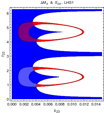
Figure 2: Ranges for $\Delta M_{s}$ (red region) and $S_{\psi\phi}$ (blue region) for $M_{H}=1$ TeV in LHS1 satisfying the bounds in Eq. (127).

 

Comparing Fig. 2 with the corresponding $Z^{\prime}$ result of Fig. 2 in [1] we observe that the phase structure is identical to the one found in the case of $Z^{\prime}$ but the values of $\tilde{s}_{23}$ are smaller. This behaviour is easy to understand. While the tree diagram with scalar exchange has the overall sign opposite to the one of a gauge boson exchange, this difference is canceled by the opposite signs of the matrix element of the leading operator $Q_{1}^{\text{SLL}}$ and $Q_{1}^{\text{VLL}}$ in the case of $H$ and $Z^{\prime}$ exchange, respectively. But the absolute value of $\langle Q_{1}^{\text{SLL}}\rangle$ is larger than of $\langle Q_{1}^{\text{VLL}}\rangle$ and consequently $\tilde{s}_{23}$ in the Higgs case has to be smaller than in the $Z^{\prime}$ case in order to fit data. We find that this suppression of $\tilde{s}_{23}$ that enters quadratically in $\Delta M_{s}$ amounts roughly to a factor of $1.5$.

In view of this simple change we do not show the table for the allowed ranges for $\delta_{23}$ and $\tilde{s}_{23}$. They are obtained from Table 5 in [1] by leaving $\delta_{23}$ unchanged and rescaling $\tilde{s}_{23}$ down by a factor of $1.5$.

Inspecting Fig. 2 we observe the following pattern:

• For each oasis with a given $\delta_{23}$ there is another oasis with $\delta_{23}$ shifted by $180^{\circ}$ but the range for $\tilde{s}_{23}$ is unchanged. This discrete ambiguity results from the fact that $\Delta M_{s}$ and $S_{\psi\phi}$ are governed by $2\delta_{23}$. However, as we will see below this ambiguity can be resolved by other observables. Without the additional information on phases mentioned in connection with constraints (127)-(129) one would find two additional small oases corresponding roughly to NP contribution to $M^{s}_{12}$ twice as large as the SM one but carrying opposite sign. But taking these constraints on the phases into account removes these oases from our analysis.

• The increase of $M_{H}$ by a given factor allows to increase $\tilde{s}_{23}$ by the same factor. This structure is evident from the formulae for $\Delta S(B_{s})$. However, the inspection of the formulae for $\Delta F=1$ transitions shows that this change will have impact on rare decays, making the NP effects in them with increased $M_{H}$ smaller. This is evident from the correlations derived in Subsection 6.2.

We will next confine our numerical analysis to these oases, investigating whether some of them can be excluded by other constraints and studying correlations between various observables. To this end we consider in parallel pseudoscalar and scalar scenarios setting the lepton couplings as given in (125). In addition to the general case corresponding to the oases just discussed we will present in plots the results obtained when the $U(2)^{3}$ symmetry is imposed on $B_{s}$ and $B_{d}$ systems. This case will be discussed in detail at the end of this subsection but to avoid too many plots and to show the impact of this symmetry we will already include the results in discussing the results without this symmetry. Our colour coding will be as follows:

• In the general case blue and purple allowed regions correspond to oases with small and large $\delta_{23}$, respectively. However, one should keep in mind the next comment.

• In the $U(2)^{3}$ symmetry case, the allowed region will be in magenta and and cyan for LHS1 and LHS2, respectively, as in this case even in the $B_{s}$ system there is dependence on $|V_{ub}|$ scenario. These regions are subregions of the general blue or purple regions so that they cover some parts of them.

In order to justify the values for the leptonic couplings in (125) we show in Fig. 3 $\overline{R}$ as function of $\tilde{\Delta}_{P}^{\mu\bar{\mu}}$ and $\Delta_{S}^{\mu\bar{\mu}}$ in LHS1 for the pseudoscalar and scalar scenario, respectively. In ALRS effects are smaller and in LRS $\overline{R}$ does not depend on $\tilde{\Delta}_{P}^{\mu\bar{\mu}}$ and $\Delta_{S}^{\mu\bar{\mu}}$. We observe that for equal scalar and pseudoscalar couplings, the effects are significantly larger in the $A^{0}$ case and this is the reason why we have chosen the scalar couplings to be larger.

There are two striking differences between $A^{0}$ and $H^{0}$ cases originating in the fact that pseudoscalar contributions interfere with the SM contribution, while this is not the case for a scalar:

• While in the $H^{0}$ case $\overline{R}$ can only be enhanced, it can also be suppressed in the $A^{0}$ case. This difference could play an important role one day.

• In the $A^{0}$ case the result depends on the oasis considered and the sign of $\tilde{\Delta}_{P}$. However changing simultaneously the sign of $\tilde{\Delta}_{P}$ and the oasis leaves $\overline{R}$ invariant. In the $H^{0}$ case $\overline{R}$ is independent of the oasis considered and of the sign of $\tilde{\Delta}_{S}$.

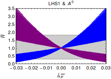
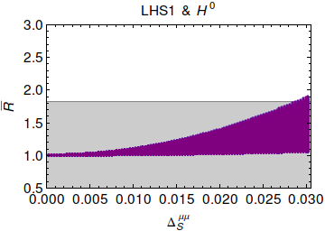
Figure 3: $\overline{R}$ as a function of $\tilde{\Delta}_{P}^{\mu\bar{\mu}}$ and $\Delta_{S}^{\mu\bar{\mu}}$ in LHS1. Left: $A^{0}$ case; right: $H^{0}$ case. Gray region: 95% CL of $R$.

 

In Fig. 4 (left) we show $S^{s}_{\mu^{+}\mu^{-}}$ vs $S_{\psi\phi}$ in the $A^{0}$ case. In the same figure (right) we show the correlation between $\overline{\mathcal{B}}(B_{s}\to\mu^{+}\mu^{-})$ and $S_{\psi\phi}$. We observe that for largest allowed values of $S_{\psi\phi}$ the asymmetry $S^{s}_{\mu^{+}\mu^{-}}$ can be as large as $\pm 0.5$. Also the effects in $\overline{\mathcal{B}}(B_{s}\to\mu^{+}\mu^{-})$ are expected to be sizable for the chosen value of muon coupling.

Comparing the plots in Fig. 4 with the corresponding results for $Z^{\prime}$ in Fig. 3 of [1] we observe striking differences which allow to distinguish the case of tree-level pseudoscalar exchange from the heavy gauge boson exchange:

• In the $A^{0}$ case the asymmetry $S^{s}_{\mu^{+}\mu^{-}}$ can be zero while this was not the case in the $Z^{\prime}$ case where the requirement of suppression of $\Delta M_{s}$ directly translated in $S^{s}_{\mu^{+}\mu^{-}}$ being non-zero. Consequently in the $Z^{\prime}$ case the sign of $S^{s}_{\mu^{+}\mu^{-}}$ could be used to identify the right oasis. The left plot in Fig. 4 clearly shows that this is not possible in the $A^{0}$ case. We also find that while in the $Z^{\prime}$ case the asymmetry $S^{s}_{\mu^{+}\mu^{-}}$ could reach values as high as $\pm 0.9$, in the $A^{0}$ case $|S^{s}_{\mu^{+}\mu^{-}}|$ can hardly be larger than 0.5.

• On the other hand we observe that in the $A^{0}$ case the measurement of $\overline{\mathcal{B}}(B_{s}\to\mu^{+}\mu^{-})$ uniquely chooses the right oasis. The enhancement of this branching ratio relatively to the SM chooses the blue oasis while the suppression the purple one. This was not possible in the $Z^{\prime}$ case. The maximal enhancements and suppressions are comparable in both cases but finding $\overline{\mathcal{B}}(B_{s}\to\mu^{+}\mu^{-})$ close to SM value would require in the $A^{0}$ case either larger $M_{H}$ or smaller muon coupling.

We observe that the roles of $S^{s}_{\mu^{+}\mu^{-}}$ and $\overline{\mathcal{B}}(B_{s}\to\mu^{+}\mu^{-})$ in searching for optimal oasis have been interchanged when going from the $Z^{\prime}$ case to the $A^{0}$ case. While $\overline{\mathcal{B}}(B_{s}\to\mu^{+}\mu^{-})$ identifies the oasis the correlation of $S^{s}_{\mu^{+}\mu^{-}}$ vs. $S_{\psi\phi}$ constitutes an important test of the model. While in the blue oasis $S_{\psi\phi}$ increases (decreases) uniquely with increasing (decreasing) $S^{s}_{\mu^{+}\mu^{-}}$ , in the purple oasis, the increase of $S_{\psi\phi}$ implies uniquely a decrease of $S^{s}_{\mu^{+}\mu^{-}}$. Therefore, while $S^{s}_{\mu^{+}\mu^{-}}$ alone cannot uniquely determine the optimal oasis, it can do in collaboration with $S_{\psi\phi}$.

If the favoured oasis will be found to differ from the one found by means of $\overline{\mathcal{B}}(B_{s}\to\mu^{+}\mu^{-})$ one day the model in question will be in trouble. Indeed, let us assume that $\overline{\mathcal{B}}(B_{s}\to\mu^{+}\mu^{-})$ will be found above its SM value selecting thereby blue oasis. Then the measurement of $S_{\psi\phi}$ will uniquely predict the sign of $S^{s}_{\mu^{+}\mu^{-}}$. Moreover, in the case of $S^{s}_{\psi\phi}$ sufficiently different from zero, we will be able to determine not only the sign but also the magnitude of $S^{s}_{\mu^{+}\mu^{-}}$.

Figure 4: $S^{s}_{\mu^{+}\mu^{-}}$ versus $S_{\psi\phi}$ (left) and $S_{\psi\phi}$ versus $\overline{\mathcal{B}}(B_{s}\to\mu^{+}\mu^{-})$ (right) for $M_{H}=1~{}$TeV in LHS for two oases as explained in the text and $A^{0}$ case. The blue and purple regions are almost identical for LHS1 and LHS2. The magenta region corresponds to the $U(2)^{3}$ limit for LHS1 and the cyan region for LHS2 (see Sect. 8.1.3). Gray region: exp 1$\sigma$ range $\overline{\mathcal{B}}(B_{s}\to\mu^{+}\mu^{-})=(3.2^{+1.5}_{-1.2})\cdot 10^{-9}$. Red point: SM central value.

 

These striking differences between the $A^{0}$-scenario and $Z^{\prime}$-scenario can be traced back to the difference between the phase of the NP correction to $P$ in these two NP scenarios. As the oasis structure as far as the phase $\delta_{23}$ is concerned is the same in both scenarios the difference enters through the muon couplings which are imaginary in the case of $A^{0}$-scenario but real in the case of $Z^{\prime}$. This is in fact the main reason why the structure of correlations in both scenarios is so different. Taking in addition into account the sign difference between $Z^{\prime}$ and pseudoscalar propagator in the the $b\to s\mu^{+}\mu^{-}$ amplitude, which is now not compensated by a hadronic matrix element, we find that

$$P(Z^{\prime})=1+r_{Z^{\prime}}e^{i\delta_{Z^{\prime}}},\qquad P(A^{0})=1+r_{A^{0}}e^{i\delta_{A^{0}}}$$ (130)

with

$$r_{Z^{\prime}}\approx r_{A^{0}},\qquad\delta_{Z^{\prime}}=\delta_{23}-\beta_{s},\qquad\delta_{A^{0}}=\delta_{Z^{\prime}}-\frac{\pi}{2}.$$ (131)

Therefore with $\delta_{23}$ of Fig. 2 the phase $\delta_{Z^{\prime}}$ is around $90^{\circ}$ and $270^{\circ}$ for the blue and purple oasis, respectively. Correspondingly $\delta_{A^{0}}$ is around $0^{\circ}$ and $180^{0}$. This difference in the phases is at the origin of the differences listed above. In particular, we understand now why the CP asymmetry $S^{s}_{\mu^{+}\mu^{-}}$ can vanish in the $A^{0}$ case, while it was always different from zero in the $Z^{\prime}$-case. What is interesting is that this difference is just related to the different particle exchanged: gauge boson and pseudoscalar. We summarize the ranges of $\delta_{Z^{\prime}}$ and $\delta_{A^{0}}$ in Table 6.

Oasis	$\delta_{Z^{\prime}}$	$\delta_{A^{0}}$
$B_{s}$ (blue)	$50^{\circ}-130^{\circ}$	$-40^{\circ}-(+40^{\circ})$
$B_{s}$ (purple)	$230^{\circ}-310^{\circ}$	$140^{\circ}-220^{\circ}$
$B_{d}$ (S1) (yellow)	$57^{\circ}-86^{\circ}$	$-33^{\circ}-(+4^{\circ})$
$B_{d}$ (S1) (green)	$237^{\circ}-266^{\circ}$	$147^{\circ}-176^{\circ}$
$B_{d}$ (S2) (yellow)	$103^{\circ}-125^{\circ}$	$13^{\circ}-35^{\circ}$
$B_{d}$ (S2) (green)	$283^{\circ}-305^{\circ}$	$193^{\circ}-215^{\circ}$
$U(2)^{3}$ (S1) (blue, magenta)	$55^{\circ}-84^{\circ}$	$-35^{\circ}-(-6^{\circ})$
$U(2)^{3}$ (S1) (purple, magenta)	$235^{\circ}-264^{\circ}$	$145^{\circ}-174^{\circ}$
$U(2)^{3}$ (S2) (blue, cyan)	$101^{\circ}-121^{\circ}$	$11^{\circ}-31^{\circ}$
$U(2)^{3}$ (S2) (purple, cyan)	$291^{\circ}-301^{\circ}$	$201^{\circ}-211^{\circ}$

Table 6: Ranges for the values of $\delta_{Z^{\prime}}$ and $\delta_{A^{0}}$ as defined in (130) for the $B_{s}$ and $B_{d}$ systems and various cases discussed in the text. Also the result for $U(2)^{3}$ models is shown.

 

Figure 5: $S^{s}_{\mu^{+}\mu^{-}}$ versus $S_{\psi\phi}$ (left) and $S_{\psi\phi}$ versus $\overline{\mathcal{B}}(B_{s}\to\mu^{+}\mu^{-})$ (right) for $M_{H}=1~{}$TeV in LHS1 for two oases as explained in the text and $H^{0}$ case (the two oases overlap here).The magenta region corresponds to the $U(2)^{3}$ limit for LHS1 and the cyan region for LHS2. Gray region: exp 1$\sigma$ range $\overline{\mathcal{B}}(B_{s}\to\mu^{+}\mu^{-})=(3.2^{+1.5}_{-1.2})\cdot 10^{-9}$. Red point: SM central value.

 

The power of the correlations in question in distinguishing between various scenarios is further demonstrated when we consider the case of a scalar in which there is no interference with the SM contribution. In Fig. 5 we show the corresponding results in the $H^{0}$ case. We observe the following differences with respect to Fig. 4:

• $\overline{\mathcal{B}}(B_{s}\to\mu^{+}\mu^{-})$ can only be enhanced in this scenario and this result is independent of the oasis considered. Thus finding this branching ratio below its SM value would favour the pseudoscalar scenario over scalar one. But the enhancement is not as pronounced as in the pseudoscalar case because the correction to the branching ratio is governed here by the square of the muon coupling while in the pseudoscalar case the correction was proportional to this coupling due to the interference with the SM contribution which is absent here.

• Concerning CP-asymmetries similarly to the branching ratio there is no dependence on the oasis considered but more importantly $S^{s}_{\mu^{+}\mu^{-}}$ can only increase with increasing $S_{\psi\phi}$.

It is instructive to understand better the results in the scalar scenario. Inspecting the formulae for the Wilson coefficients we arrive at an important relation:

$$\varphi_{S}=\delta_{Z^{\prime}}-\pi,$$ (132)

where the shift is related to the minus sign difference in the $Z^{\prime}$ and scalar propagators.

But as seen in (4.5) the three observables given there, all depend on $2\varphi_{S}$, implying that from the point of view of these quantities this shift is irrelevant. As different oases correspond to phases shifted by $\pi$ this also explains why in the scalar case the results in different oases are the same. That the branching ratio can only be enhanced follows just from the absence of the interference with the SM contributions. In order to understand the signs in $S_{\mu\mu}^{s}$ one should note the minus sign in front of sine in the corresponding formula. Rest follows from (132) and Table 6.

Figure 6: $\mathcal{A}^{\lambda}_{\Delta\Gamma}$ versus $S_{\psi\phi}$ for $M_{H}=1~{}$TeV in LHS1, blue and purple oases and $A^{0}$ case (left) and $H^{0}$ case (right). In $H^{0}$ case the two oases overlap. The magenta region corresponds to the $U(2)^{3}$ limit for LHS1 and the cyan region for LHS2. Red point: SM central value.

 

In Fig. 6 we plot $\mathcal{A}^{\lambda}_{\Delta\Gamma}$ vs $S_{\psi\phi}$ for $A^{0}$ and $H^{0}$ cases. We observe that for $M_{H}=1\,{\rm TeV}$, even for $S_{\psi\phi}$ significantly different from zero, $\mathcal{A}^{\lambda}_{\Delta\Gamma}$ does not defer significantly from unity in both scenarios. Larger effects have been found in the $Z^{\prime}$ case as seen Fig. 4 of [1].

Figure 7: $S^{s}_{\mu^{+}\mu^{-}}$ versus $S_{\psi\phi}$ (left) and $S_{\psi\phi}$ versus $\overline{\mathcal{B}}(B_{s}\to\mu^{+}\mu^{-})$ (right) for $M_{H}=1~{}$TeV in LHS1 for two oases and the mixed $H^{0}$ and $A^{0}$ case with $\Delta_{S}^{\mu\bar{\mu}}=2\tilde{\Delta}_{P}^{\mu\bar{\mu}}$. The magenta region corresponds to the $U(2)^{3}$ limit for LHS1 and the cyan region for LHS2. Gray region: exp 1$\sigma$ range $\overline{\mathcal{B}}(B_{s}\to\mu^{+}\mu^{-})=(3.2^{+1.5}_{-1.2})\cdot 10^{-9}$. Red point: SM central value.

 

In Fig. 7 we show how the plots in Figs. 4 and 5 change when the exchanged particle has both scalar and pseudoscalar couplings to muons with

$$\Delta_{S}^{\mu\bar{\mu}}=2\tilde{\Delta}_{P}^{\mu\bar{\mu}}=0.4\frac{m_{b}(M_{H})}{m_{b}(m_{b})}.$$ (133)

We observe that while the correlation between $S^{s}_{\mu^{+}\mu^{-}}$ and $S_{\psi\phi}$ is relative to $A^{0}$ case practically unmodified, the correlation between $S_{\psi\phi}$ and $\overline{\mathcal{B}}(B_{s}\to\mu^{+}\mu^{-})$ is visibly modified for $\overline{\mathcal{B}}(B_{s}\to\mu^{+}\mu^{-})$ below the SM value while less if an enhancement is present.

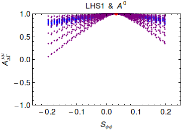
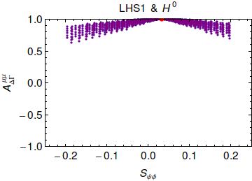
Figure 8: Correlation plots as in Fig. 4, 5, and 6 but now with lepton coupling $\tilde{\Delta}_{P}\in[0.02,0.04]$, $\Delta_{S}=0$ (left) and $\Delta_{S}\in[0.02,0.04]$, $\tilde{\Delta}_{P}=0$ (right) in LHS1. Gray region: exp 1$\sigma$ range $\overline{\mathcal{B}}(B_{s}\to\mu^{+}\mu^{-})=(3.2^{+1.5}_{-1.2})\cdot 10^{-9}$. Red point: SM central value.

 

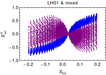
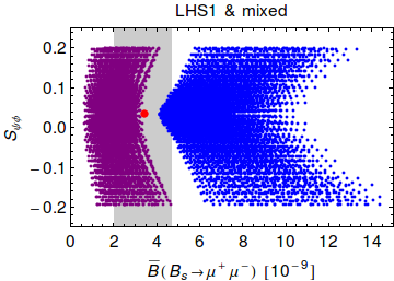
Figure 9: Correlation plots as in Fig. 7 but now with $\tilde{\Delta}_{P}\in[0.02,0.04]$ and $\Delta_{S}\in[0.02,0.04]$. Gray region: exp 1$\sigma$ range $\overline{\mathcal{B}}(B_{s}\to\mu^{+}\mu^{-})=(3.2^{+1.5}_{-1.2})\cdot 10^{-9}$. Red point: SM central value.

 

Clearly for a fixed $M_{H}$ the results presented so far depend on the choice on muon couplings made by us. In Figs. 8 and 9 we show the corresponding plots when the lepton couplings $\tilde{\Delta}_{P}$ and $\Delta_{S}$ are varied independently in the range $0.02-0.04$. Evidently, the allowed regions are now larger but the general pattern of correlations remains. These results are presented here only for illustration and we will not discuss this mixed scenario for other meson systems.

8.1.2 The $B_{d}$ Meson System

We begin by searching for the allowed oases in this case. The result is shown in Fig. 10. The general structure of the discrete ambiguities is as in the $B_{s}$ case but now as expected the selected oases in S1 and S2 differ significantly from each other. In fact this figure has the same phase structure as Fig. 6 in [1] except that the allowed values of $\tilde{s}_{13}$ are reduced with respect to the $Z^{\prime}$ case for the same reason as in the $B_{s}$ system: the relevant hadronic matrix elements are larger.

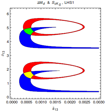
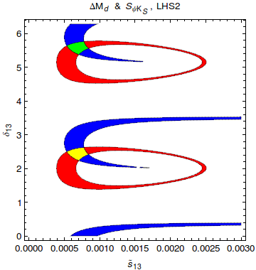
Figure 10: Ranges for $\Delta M_{d}$ (red region) and $S_{\psi K_{S}}$ (blue region) for $M_{H}=1$ TeV in LHS1 (left) and LHS2 (right) satisfying the bounds in Eq. (128).

 

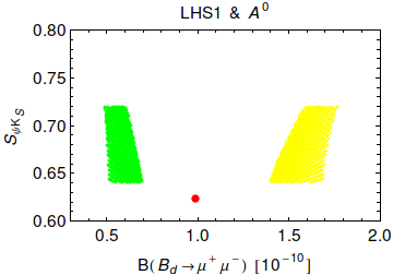
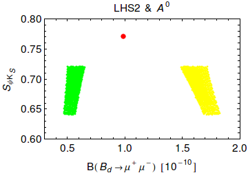
Figure 11: $S_{\psi K_{S}}$ versus $\mathcal{B}(B_{d}\to\mu^{+}\mu^{-})$ in $A^{0}$ scenario for $M_{H}=1$ TeV in LHS1 (left) and LHS2 (right) in the yellow and green oases as discussed in the text. Red point: SM central value.

 

Let us first concentrate on S2 scenario and the $A^{0}$ case. Our colour coding is such that

• In the general case yellow and green allowed regions correspond to oases with small and large $\delta_{13}$, respectively.

• In principle in the $U(2)^{3}$ symmetry case we could again show the reduced regions with magenta and cyan for LHS1 and LHS2, respectively but this reduction amounts typically to $5-10\%$ at most and it is more transparent not to show it. This small impact of $U(2)^{3}$ symmetry in the $B_{d}$ system is evident from Table 6.

In the right panel of Fig. 11 we show $S_{\psi K_{S}}$ vs $\mathcal{B}(B_{d}\to\mu^{+}\mu^{-})$. This result should be compared with the one for $Z^{\prime}$ case shown in the right panel of Fig. 7 in [1].

In order to understand the differences between these two scenarios of NP we again look at the phase of the correction to $P$ which now is given as follows:

$$r_{Z^{\prime}}\approx r_{A^{0}},\qquad\delta_{Z^{\prime}}=\delta_{13}-\beta,\qquad\delta_{A^{0}}=\delta_{Z^{\prime}}-\frac{\pi}{2}.$$ (134)

Note that this time the phase of $V_{td}$ enters the analysis with $\beta\approx 19^{\circ}$ and $\beta\approx 25^{\circ}$ for S1 and S2 scenario of $|V_{ub}|$, respectively. We find then that in scenario S2 the phase $\delta_{Z^{\prime}}$ is around $115^{\circ}$ and $295^{\circ}$ for yellow and green oases, respectively. Correspondingly $\delta_{A^{0}}$ is around $25^{\circ}$ and $205^{\circ}$. We summarize the ranges of $\delta_{Z^{\prime}}$ and $\delta_{A^{0}}$ in Table 6.

With this insight at hand we can easily understand the plots in question noting that the enhancements and suppressions of $\mathcal{B}(B_{d}\to\mu^{+}\mu^{-})$ are governed by the cosine of the phase of the correction:

• In the $A^{0}$ case $\mathcal{B}(B_{d}\to\mu^{+}\mu^{-})$ is enhanced in the yellow oasis but suppressed in the green oasis.

• In the $Z^{\prime}$-case the behaviour is opposite: $\mathcal{B}(B_{d}\to\mu^{+}\mu^{-})$ is suppressed in the yellow oasis but enhanced in the green oasis.

• For the choice of parameters NP effects are a bit larger in the $A^{0}$ case.

Note that in both cases the requirement on $S_{\psi K_{S}}$ and $\Delta M_{d}$ forces $\mathcal{B}(B_{d}\to\mu^{+}\mu^{-})$ to differ from the SM value. In the $A^{0}$ case these enhancements and suppressions amount up to $\pm 70\%$ for $M_{H}=1\,{\rm TeV}$. They increase with decreasing $S_{\psi K_{S}}$.

Note that because of the correlation between $\mathcal{B}(B_{d}\to\mu^{+}\mu^{-})$ and $S_{\psi K_{S}}$ and the fact that the latter is already well determined, the range of $\delta_{13}$ cannot be large and consequently also the ranges for the phases $\delta_{Z^{\prime}}$ and $\delta_{A^{0}}$ are small allowing thereby the identification of the right oasis by $\mathcal{B}(B_{d}\to\mu^{+}\mu^{-})$ only.

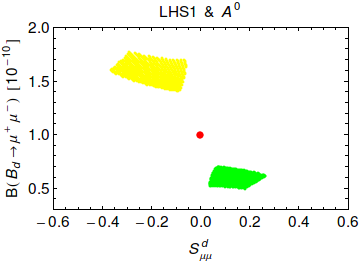
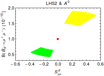
Figure 12: $\mathcal{B}(B_{d}\to\mu\bar{\mu})$ versus $S_{\mu^{+}\mu^{-}}^{d}$ in $A^{0}$ case for $M_{Z^{\prime}}=1$ TeV in LHS1 (left) and LHS2 (right) for the green and yellow oases as discussed in the text. Red point: SM central value.

 

While the correlation between $\mathcal{B}(B_{d}\to\mu^{+}\mu^{-})$ and $S_{\psi K_{S}}$ offers a distinction between $Z^{\prime}$ and pseudoscalar scenario even more interesting in this respect is the correlation between $\mathcal{B}(B_{d}\to\mu^{+}\mu^{-})$ and $S_{\mu^{+}\mu^{-}}^{d}$. We show this correlation in Fig. 12 (right panel). Comparing this result with right panel of Fig. 8 in [1] we observe that in LHS2 these two observables are correlated within $A^{0}$ case but anticorrelated in the $Z^{\prime}$ scenario. Also this behaviour follows directly from the phase structure of NP contributions in these two cases. Measuring only the signs of shifts in these two observables relative to the SM values will uniquely tell us which of these two NP scenarios could be at work and which not.

We next turn to LHS1 scenario for $|V_{ub}|$. We observe that the phase $\delta_{13}$ is lower than in the case of scenario S2 but $\tilde{s}_{13}$ is basically the same. Using (134) we can again calculate the phases of NP physics contributions to $P$. We find that now $\delta_{Z^{\prime}}$ is around $70^{\circ}$ and $250^{\circ}$ for yellow and green oases, respectively. Correspondingly $\delta_{A^{0}}$ is around $-20^{\circ}$ and $160^{\circ}$. We summarize the ranges of $\delta_{Z^{\prime}}$ and $\delta_{A^{0}}$ in Table 6.

With this insight at hand we can easily understand the plots in the left panels in Figs. 11 and 12 and analogous plots in the left panels of Figs. 7 and 8 in [1]. In particular as seen in Fig. 12 there is a flip in sign of $S^{d}_{\mu^{+}\mu^{-}}$ when moving from LHS1 to LHS2 while there is no qualitative change in the case of $\mathcal{B}(B_{d}\to\mu^{+}\mu^{-})$. The opposite behaviour is found in the $Z^{\prime}$ case.

Therefore what distinguishes LHS1 from LHS2 in both NP scenarios is the sign of the correlation between $S^{d}_{\mu^{+}\mu^{-}}$ and $\mathcal{B}(B_{d}\to\mu^{+}\mu^{-})$. In the $A^{0}$ case a positive $S^{d}_{\mu^{+}\mu^{-}}$ implies suppression of $\mathcal{B}(B_{d}\to\mu^{+}\mu^{-})$ in LHS1 but enhancement in LHS2. Note that this pattern is independent of the sign of $\tilde{\Delta}_{P}^{\mu\bar{\mu}}$ coupling as this coupling enters both observables. On the other hand the flip of this sign would interchange colours in Figs. 11 and 12. As seen in Figs. 7 and 8 in [1] in the $Z^{\prime}$-case the behaviour is opposite to the one found in the $A^{0}$ case: anti-correlation in LHS1 and correlation in LHS2 between $S^{d}_{\mu^{+}\mu^{-}}$ and $\mathcal{B}(B_{d}\to\mu^{+}\mu^{-})$ in the $A^{0}$ case is changed respectively to correlation and anti-correlation in the $Z^{\prime}$-case. This means again that once we will know whether LHS1 or LHS2 is chosen by nature the measurements of $S^{d}_{\mu^{+}\mu^{-}}$ and $\mathcal{B}(B_{d}\to\mu^{+}\mu^{-})$ will tell us which of the two NP scenarios are favoured. However, we are aware of the fact that while the measurement of $S^{s}_{\mu^{+}\mu^{-}}$ is extremely difficult, the measurement of $S^{d}_{\mu^{+}\mu^{-}}$ will require heroic efforts and it may take decades to realize such a measurement.

We next move to consider the $H^{0}$ case and show the results in this case in Figs. 13 and 14 that correspond to Figs. 11 and 12 in the $A^{0}$ case, respectively. We observe the following differences between $A^{0}$ and $H^{0}$ cases:

• As in the case of $B_{s}\to\mu^{+}\mu^{-}$ there is no dependence on the oasis considered and in all plots in Figs. 13 and 14 $\mathcal{B}(B_{d}\to\mu^{+}\mu^{-})$ is always enhanced as opposed to the $A^{0}$ case where it could also be suppressed.

• The asymmetry $S^{d}_{\mu^{+}\mu^{-}}$ is negative and positive in LHS1 and LHS2, respectively, while in the $A^{0}$ case both signs were possible in LHS1 and LHS2.

In order to understand the signs of $S^{d}_{\mu^{+}\mu^{-}}$ in this case one should just use Table 6 and the relation (132) in the $B_{d}$ system. Effectively these signs in Figs. 13 and 14 can be obtained from the corresponding plots in Figs. 11 and 12 by simply removing the regions with suppression of $\mathcal{B}(B_{d}\to\mu^{+}\mu^{-})$. Therefore the distinction between $S$ and $P$ will only be easy if this branching ratio will turn out to be suppressed with respect to its SM value.

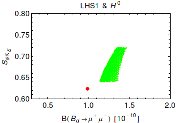
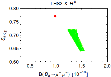
Figure 13: $S_{\psi K_{S}}$ versus $\mathcal{B}(B_{d}\to\mu^{+}\mu^{-})$ in $H^{0}$ scenario for $M_{H}=1$ TeV in LHS1 (left) and LHS2 (right) in the yellow and green oases that overlap here. Red point: SM central value.

 

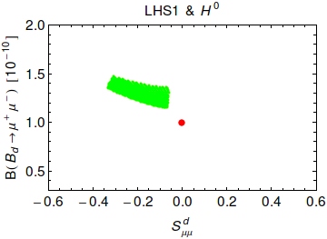
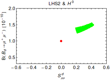
Figure 14: $\mathcal{B}(B_{d}\to\mu\bar{\mu})$ versus $S_{\mu^{+}\mu^{-}}^{d}$ in $H^{0}$ case for $M_{H}=1$ TeV in LHS1 (left) and LHS2 (right) for the green and yellow oases (they overlap here) as discussed in the text. Red point: SM central value.

 

8.1.3 The $U(2)^{3}$ Limit

We have investigated how the results presented until now are modified when the flavour $U(2)^{3}$ symmetry [74, 75, 76, 77, 78, 79, 80] is imposed on the $H$ couplings. As pointed out in [9] in this case $\varphi_{B_{d}}=\varphi_{B_{s}}$ which in turn implies not only the correlation between CP asymmetries $S_{\psi K_{S}}$ and $S_{\psi\phi}$ but also a triple $S_{\psi K_{S}}-S_{\psi\phi}-|V_{ub}|$ correlation.

Usually, when considering the case of $U(2)^{3}$ broken by the minimal set of spurions, the $MU(2)^{3}$ case, only SM operators are involved. Yet, as mentioned in [9] in the case of ${\rm 2HDM_{\overline{\rm MFV}}}$ [81] with flavour blind phases dominantly in the Higgs potential and the dominance of scalar left-handed currents also the $U(2)^{3}$ structure of scalar contributions to FCNC transitions is obtained. Thus only the LHS1 and LHS2 scenarios are involved in this case. In what follows we will confine our discussion to $B_{s}$ and $B_{d}$ systems as NP effects in the $K$ system are much less interesting in the NP scenarios considered in this paper. General discussion can be found in [9].

Until now NP effects in the observables in $B_{d}$ and $B_{s}$ systems where uncorrelated but now they are correlated with each other due to the relations:

$$\frac{\tilde{s}_{13}}{|V_{td}|}=\frac{\tilde{s}_{23}}{|V_{ts}|},\qquad\delta_{13}-\delta_{23}=\beta-\beta_{s}.$$ (135)

Thus, once the allowed oases in the $B_{d}$ system are fixed, the oases in $B_{s}$ system are determined. Moreover, all observables in both systems are described by only one real positive parameter and one phase, e.g. $({\tilde{s}}_{23},\delta_{23})$.

We also have in this case [9]

$$S^{s}_{\mu^{+}\mu^{-}}=S^{d}_{\mu^{+}\mu^{-}}$$ (136)

for which formulae in the $H^{0}$ and $A^{0}$ case can be found in Subsection 4.5.

In Fig. 15 we combine Figs. 2 and 10 using the $U(2)^{3}$ symmetry relations in (135). In the $U(2)^{3}$ limit the allowed oases get smaller. This decrease turns out to be not very pronounced in the case of $({\tilde{s}}_{13},\delta_{13})$ oases as they were already small as seen in Fig. 10 but has a significant impact on $({\tilde{s}}_{23},\delta_{23})$ oases which where much larger as seen in Fig. 2. Moreover the fact that the results in the $B_{d}$ system depend on whether LHS1 or LHS2 is considered is now transfered through the relations in (135) into the $B_{s}$ system. This is clearly seen in Fig. 15, in particular the final oases in cyan in LHS2 are visibly smaller than the magenta oases in LHS1 due to the required shift of $S_{\psi K_{S}}$.

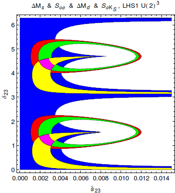
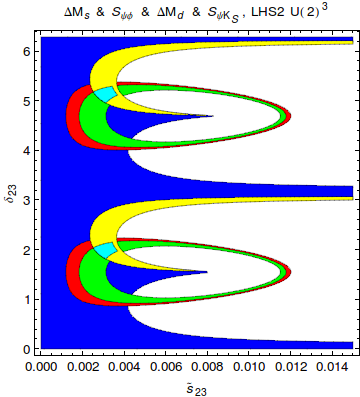
Figure 15: Ranges for $\Delta M_{s}$ (red region), $S_{\psi\phi}$ (blue region), $\Delta M_{d}$ (green region) and $S_{\psi K_{S}}$ (yellow region)for $M_{H}=1$ TeV in LHS1 (left) and LHS2 (right) in the $U(2)^{3}$ limit satisfying the bounds in Eq. (127) and  (128). The overlap region of all four regions is shown in magenta in LHS1 and in cyan in LHS2.

 

Inspecting the ranges for the phases in the last four rows of Table 6, which now apply to both $B_{s}$ and $B_{d}$ systems and comparing them with the remaining rows of these tables we can predict the impact of the imposition of $U(2)^{3}$ symmetry on the results in both systems presented so far:

• In the case of $B_{s}$ system in which previously there was no distinction between LHS1 and LHS2 the changes are as follows. The plots in Figs. 4 and 5 still apply but the allowed regions get smaller and some of them are valid only for LHS1 (magenta) and other for LHS2 (cyan). We also note that the imposition of $U(2)^{3}$ symmetry favours regions away from the SM point.

• In the $B_{d}$ system the plots in Figs. 11–14 have the same structure as previously and as stated previously the effect of the imposition of $U(2)^{3}$ symmetry is so small that we do not show magenta and cyan areas in this case. They would cover almost completely the yellow and green areas, respectively.

These expectations could be already made by comparing the right panel of Fig. 3 and Fig. 25 in [1] in the case of $Z^{\prime}$ scenario. Indeed also there the imposition of $U(2)^{3}$ symmetry reduces the allowed ranges significantly in the $B_{s}$ system and make a clear distinction between LHS1 and LHS2 scenario which was absent previously. We see again how important the determination of $|V_{ub}|$ is. Knowing future precise values of $|V_{ub}|$ as well as $S_{\psi\phi}$ and $\mathcal{B}(B_{s,d}\to\mu^{+}\mu^{-})$ will confirm or rule out this scenario of NP. These correlations are particular examples of the correlations in $MU(2)^{3}$ models pointed out in [9]. What is new here is that in a specific model considered by us the $|V_{ub}|-S_{\psi\phi}$ correlation has now also implications for $\overline{\mathcal{B}}(B_{s}\to\mu^{+}\mu^{-})$ and $S_{\mu\mu}^{s}$.

In Fig. 16 we show $\mathcal{B}(B_{d}\to\mu^{+}\mu^{-})$ versus $\overline{\mathcal{B}}(B_{s}\to\mu^{+}\mu^{-})$ for the $A^{0}$ and $H^{0}$ cases. As expected on the basis of a general discussion in [9] there is a very strong correlation between these two branching ratios. Again, while in the $A^{0}$ case both branching ratios can be enhanced or suppressed with respect to the SM, they can be only enhanced in the $H^{0}$ case.

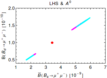
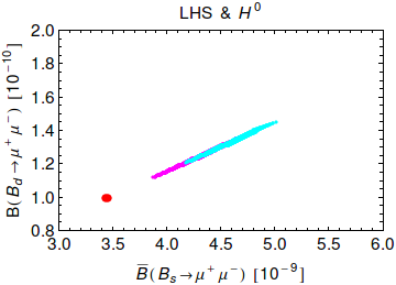
Figure 16: $\mathcal{B}(B_{d}\to\mu^{+}\mu^{-})$ versus $\overline{\mathcal{B}}(B_{s}\to\mu^{+}\mu^{-})$ for $M_{H}=1$ TeV in $A^{0}$ case (left) and $H^{0}$ case (right) in the $U(2)^{3}$ limit satisfying the bounds in Eq. (127) and  (128).

 

8.2 The RHS1 and RHS2 Scenarios

8.2.1 First Observations

We will now investigate $H$ scenario with exclusively RH couplings to quarks. Now in the RHS1 and RHS2 scenarios only RH couplings to quarks are present in $H$ contributions. As QCD is parity conserving, the hadronic matrix elements for operators with RH currents as well as QCD corrections remain unchanged. The expressions for $\Delta F=2$ observables in RHS1 and RHS2 scenarios as well as the corresponding constraints have precisely the same structure as in the LHS1 and LHS2 cases just discussed. Therefore the oases in the space of parameters related to RH currents are precisely the same as in LHS1 and LHS2 scenarios, except that the parameters $\tilde{s}_{ij}$ and $\delta_{ij}$ parametrize now RH and not LH currents. Anticipating this result we have not introduced separate description of LH and RH oases. Yet, in the case of $\Delta F=1$ observables several changes are present which allow in principle to distinguish the RHS1 and RHS2 scenarios from the corresponding LHS1 and LHS2 scenarios.

8.2.2 The $B_{s}$ Meson System

On the left in Figs. 4 and  5 we have shown $S^{s}_{\mu^{+}\mu^{-}}$ vs $S_{\psi\phi}$ in the LHS1 scenario for $A^{0}$ and $H^{0}$ cases, respectively. Analogous plots for the correlation of $S_{\psi\phi}$ vs $\overline{\mathcal{B}}(B_{s}\to\mu^{+}\mu^{-})$ in the LHS1 scenario are shown in Figs. 4 and 5. Inspecting the related formulae for RHS scenario we conclude similarly to the $Z^{\prime}$ case that in the case of $A^{0}$ these plots are also valid for RHS1 scenario except that the colours should be interchanged. Therefore on the basis of observables considered here it is not possible to distinguish between LHS1 and RHS1 scenarios because in the RHS1 scenario one can simply interchange the two oases to obtain the same physical results as in LHS1 scenario. We also note that reversing simultaneously the sign of $\tilde{\Delta}_{P}$ would keep also the oases unchanged.

The situation is even simpler in the case of $H^{0}$ case. As the plots in question did not depend on oasis considered, the correlations in this case are identical in RHS1 and LHS1 independently of oasis considered.

Clearly as in the LHS1 scenario this result represents a test of the RHS1 scenario but if one day we will have precise measurements of $S^{s}_{\mu^{+}\mu^{-}}$, $S_{\psi\phi}$ and $\overline{\mathcal{B}}(B_{s}\to\mu^{+}\mu^{-})$ we will still not be able to distinguish for instance whether we deal with LHS1 scenario in the blue oasis or RHS1 scenario in purple oasis.

In principle, one could make a distinction between LHS and RHS scenarios by considering model independent bounds from $B\to K\mu^{+}\mu^{-}$ and $B\to K^{*}\mu^{+}\mu^{-}$ on the Wilson coefficients of the scalar operators. However, as discussed in Subsection 8.5, this is presently not the case. This should be contrasted with $Z^{\prime}$ analysis in [1] where in fact such a distinction could be made.

8.2.3 The $B_{d}$ Meson System

Similarly to the $B_{s}$ case the structure of oases is as in Fig. 10. Moreover, the results in in Figs. 11 –14 are valid for RHS1 and RHS2 scenarios except that in the $A^{0}$ case the colours should be interchanged, while there is no modification in the $H^{0}$ case. Thus we cannot distinguish between LHS and RHS scenarios on the basis of considered observables. Clearly the study of $b\to d\mu^{+}\bar{\mu}^{-}$ transitions could help in this context but they are more challenging both theoretically and experimentally.

8.3 The LRS1 and LRS2 Scenarios

8.3.1 First Observations

If both LH and RH currents are present in NP contributions, the pattern of flavour violation can differ from the scenarios considered until now in a profound manner. If the LH and RH couplings differ from each other, the number of parameters increases and it is harder to get clear cut conclusions without some underlying fundamental theory. On the other hand some of the “symmetries” between LHS and RHS scenarios identified above are broken and the effect of RH currents in certain cases could in principle be better visible.

Here in order to keep the same number of parameters as in previous scenarios we will assume a left-right symmetry in the $H$-couplings to quarks. That is the LH couplings $\Delta_{L}$ are equal in magnitudes and phases to the corresponding RH couplings $\Delta_{R}$. In this manner we can also keep the same parametrization of couplings as in previous scenarios.

Before entering the details let us emphasize two new features relative to the cases in which either LH or RH couplings in NP contributions were present:

• NP contributions to $\Delta F=2$ observables receive now new LR operators, whose contributions are enhanced through renormalization group effects relative to SM operators, however as scalar LL and RR operators are also enhanced by such effects the difference between LL (RR) scenarios and LR scenario in the scalar case is much smaller than in the $Z^{\prime}$ case.

• NP contributions to $B_{d,s}\to\mu^{+}\mu^{-}$ and $K_{L}\to\mu^{+}\mu^{-}$ vanish eliminating in this manner $S^{s,d}_{\mu^{+}\mu^{-}}$ and $\mathcal{B}(B_{s,d}\to\mu^{+}\mu^{-})$ as basic observables in the identification of acceptable oases. On the other hand $B\to K^{*}\mu^{+}\mu^{-}$ and $B\to K\mu^{+}\mu^{-}$ receive still NP contributions and can help in this context.

While $S^{s,d}_{\mu^{+}\mu^{-}}$ cannot help in the identification of the optimal oasis in the LR scenarios they are non-vanishing:

$$S_{\mu^{+}\mu^{-}}^{q}=-\sin(2\varphi_{B_{q}}).$$ (137)

While rather small they offer a clean test of the LR scenarios.

8.3.2 The $B_{s}$ Meson System

We begin the search for the oases with the $B_{s}$ system proceeding with input parameters as in the previous scenarios. The result of this search for $M_{H}=1\,{\rm TeV}$ is shown in Fig. 17, where we show the allowed ranges for $(\tilde{s}_{23},\delta_{23})$. The red regions correspond to the allowed ranges for $\Delta M_{s}$, while the blue ones to the corresponding ranges for $S_{\psi\phi}$. The overlap between red and blue regions identifies the oases we were looking for.

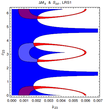
Figure 17: Ranges for $\Delta M_{s}$ (red region) and $S_{\psi\phi}$ (blue region) for $M_{H}=1$ TeV in LRS1 satisfying the bounds in Eq. (127).

 

The notations are as in previous cases but it should be kept in mind that the parameters $(\tilde{s}_{23},\delta_{23})$ describe both LH and RH couplings.

In order to understand the structure of oases in Fig. 17, that differs from the ones found so far, we note that the matrix element of the dominant $Q_{2}^{\rm LR}$ operator has the sign opposite to the dominant $Q_{1}^{\rm SLL}$ operator. Therefore, this operator naturally suppresses $\Delta M_{s}$ with the phase $\delta_{23}$ centered in the ballpark of $0^{\circ}$ and $180^{\circ}$, that is shifted down by roughly $90^{\circ}$ relatively to the LHS scenarios. As the matrix element of $Q_{2}^{\rm LR}$ is larger than that of $Q_{1}^{\rm SLL}$ operator in LHS and RHS scenarios, $\tilde{s}_{23}$ has to be sufficiently smaller to agree with data.

The crucial role in the $B_{s}$ meson system in this scenario, in the absence of NP contributions to $B_{s,d}\to\mu^{+}\mu^{-}$ decays, is now played by $B\to K^{*}\mu^{+}\mu^{-}$ and $B\to K\mu^{+}\mu^{-}$. We will discuss the latter decays at the end of this section.

8.3.3 The $B_{d}$ Meson System

The structure of oases in this case is given in Fig. 18. As we do not have $\mathcal{B}(B_{d}\to\mu^{+}\mu^{-})$ to our disposal and $b\to d\ell^{+}\ell^{-}$ decays are challenging this system is not very useful to provide tests of LRS scenarios without some fundamental theory.

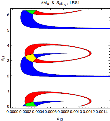
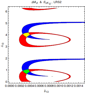
Figure 18: Ranges for $\Delta M_{d}$ (red region) and $S_{\psi K_{S}}$ (blue region) for $M_{H}=1$ TeV in LRS1 (left) and LRS2 (right) satisfying the bounds in Eq. (128).

 

Due to the sign of the matrix element of the dominant $Q_{2}^{\rm LR}$ operator in both LRS1 and LRS2 the mass difference $\Delta M_{d}$ is naturally suppressed. The requested size of this suppression together with significant suppression of $S_{\psi K_{S}}$ in LRS2 and slight enhancement of it in LRS1 governs the structure of the phases.

8.4 The ALRS1 and ALRS2 Scenarios

We include this case as well because it has not been discussed in the literature but it is an interesting NP scenario for the following reasons:

• NP contributions to $\Delta F=2$ observables are dominated as in LRS scenarios by new LR operators but as the sign of LR interference is flipped some differences arise.

• NP contributions to $B_{d,s}\to\mu^{+}\mu^{-}$ enter again with full power. Therefore these decays together with $S^{q}_{\mu^{+}\mu^{-}}$ offer as in the LHS and RHS scenarios some help in the identification of acceptable oases and to study differences between scalars, pseudoscalars and $Z^{\prime}$ bosons.

• The phase structure of the oases is as in LHS scenario but due to enhanced hadronic matrix elements of LR operators the mixing parameters $\tilde{s}_{ij}$ are decreased.

• NP contributions to $K_{L}\to\pi^{0}\ell^{+}\ell^{-}$ vanish in this scenario.

In view of this simple structure of modifications with respect to LHS scenario, all plots have the same structure as LH scenarios but NP effects are smaller. Therefore we will not show these plots.

8.5 Implications of $b\to s\ell^{+}\ell^{-}$ Constraints

Presently the NP effects found by us are consistent with the experimental data on $B_{s,d}\to\mu^{+}\mu^{-}$. However, also the data on $B\to X_{s}\ell^{+}\ell^{-}$, $B\to K^{*}\ell^{+}\ell^{-}$ and $B\to K\ell^{+}\ell^{-}$ recently improved a lot and it is of interest to see whether this has an impact on our results. It should be emphasized that $B\to X_{s}\ell^{+}\ell^{-}$, $B\to K^{*}\ell^{+}\ell^{-}$ are not as theoretically clean as $B_{s}\to\mu^{+}\mu^{-}$ because of the presence of form factors. However in the case of $B\to K\ell^{+}\ell^{-}$ progress in lattice calculations of the relevant form factors is expected soon and as stressed in particular in [16] a simultaneous consideration of this decay together with $B_{s}\to\mu^{+}\mu^{-}$ provides useful tests of extensions of the SM. Indeed, while $B_{s}\to\mu^{+}\mu^{-}$ is sensitive only to the differences $C_{P}-C_{P}^{\prime}$ and $C_{S}-C_{S}^{\prime}$, the decay $B\to K\ell^{+}\ell^{-}$ is sensitive to their sums $C_{P}+C_{P}^{\prime}$ and $C_{S}+C_{S}^{\prime}$. A very extensive model independent analysis of $C_{P}(C_{P}^{\prime})$ and $C_{S}(C_{S}^{\prime})$ in the context of the data on $B_{s}\to\mu^{+}\mu^{-}$ and $B\to K\ell^{+}\ell^{-}$ has been performed in [16]. Adjusting their normalization of Wilson coefficients to ours the final result of this paper reads:

$$m_{b}|C_{S}^{(\prime)}|\leq 0.7,\qquad m_{b}|C_{P}^{(\prime)}|\leq 1.0,$$ (138)

which implies

$$\left|\frac{1}{g_{\text{SM}}^{2}\sin^{2}\theta_{W}}\frac{1}{M_{H}^{2}}\frac{\Delta_{L,R}^{sb}(H)\Delta_{S}^{\mu\bar{\mu}}(H)}{V_{ts}^{*}V_{tb}}\right|\leq 0.70$$ (139)

$$\left|\frac{1}{g_{\text{SM}}^{2}\sin^{2}\theta_{W}}\frac{1}{M_{H}^{2}}\frac{\Delta_{L,R}^{sb}(H)\Delta_{P}^{\mu\bar{\mu}}(H)}{V_{ts}^{*}V_{tb}}\right|\leq 1.0$$ (140)

or equivalently for $M_{H}=1\,{\rm TeV}$

$$|\tilde{s}_{23}\Delta_{S}^{\mu\bar{\mu}}(H)|\leq 0.00115,$$ (141)

$$|\tilde{s}_{23}\Delta_{P}^{\mu\bar{\mu}}(H)|\leq 0.00164.$$ (142)

The largest values of $\tilde{s}_{23}$ used in our analysis are $0.0041$ in LHS and RHS scenarios with smaller values for LR and ALR scenarios. We find then $0.0001$ and $0.00005$ for the two products respectively. Therefore, these bounds do not have any impact on our results.

9 The $K$ Meson System

As we already stated previously we do not expect any visible effects in $K^{+}\rightarrow\pi^{+}\nu\bar{\nu}$ and $K_{L}\rightarrow\pi^{0}\nu\bar{\nu}$ and our discussion will concentrate on $\varepsilon_{K}$, $K_{L}\to\mu^{+}\mu^{-}$ and $K_{L}\to\pi^{0}\ell^{+}\ell^{-}$.

As seen in (129) the constraints from $\Delta F=2$ observables are weaker than in previous cases. Yet as seen in Fig. 19, obtained within LHS1 and LHS2 scenarios, it is possible to identify the allowed oases. These plots have the same phase structure as the plot in Fig. 9 of [1] for $Z^{\prime}$ scenario except that $\tilde{s}_{12}$ is by a factor of five smaller because of the enhanced matrix element of the relevant scalar operator.

Due to weaker constraints in the $K$ system the oases are rather large. We have two oases in S1:

$$C_{1}(S1):~{}~{}0^{\circ}\leq\delta_{12}\leq 90^{\circ},\qquad C_{2}(S1):~{}~{}180^{\circ}\leq\delta_{12}\leq 270^{\circ}$$ (143)

and only one oasis in S2:

$$C_{1}(S2):~{}~{}0^{\circ}\leq\delta_{12}\leq 360^{\circ}.$$ (144)

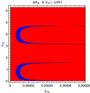
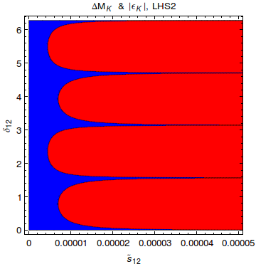
Figure 19: Ranges for $\Delta M_{K}$ (red region) and $\varepsilon_{K}$ (blue region) (LHS1: left, LHS2: right) for $M_{H}=1$ TeV satisfying the bounds in Eq. (129).

 

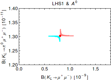
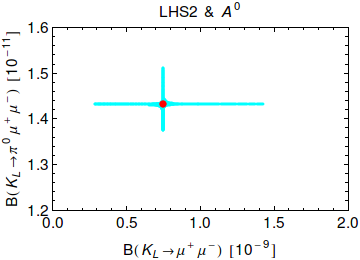
Figure 20: $\mathcal{B}(K_{L}\to\pi^{0}\mu^{+}\mu^{-})$ versus $\mathcal{B}(K_{L}\to\mu^{+}\mu^{-})$ for P scenario and LHS1 (left), LHS2 (right). Red point: SM central value.

 

With these constraints at hand we have calculated the branching ratios for $K_{L}\to\mu^{+}\mu^{-}$ and $K_{L}\to\pi^{0}\ell^{+}\ell^{-}$ decays. We can summarize our results as follows:

• NP effects in $K_{L}\to\pi^{0}e^{+}e^{-}$ are totally negligible both for $H^{0}$ and $A^{0}$ cases.

• NP effects in $K_{L}\to\pi^{0}\mu^{+}\mu^{-}$ are larger but amount to at most $\pm 5\%$ at the level of the branching ratio which is also negligibly small in view of large theoretical uncertainties.

• The short distance branching ratio for $K_{L}\to\mu^{+}\mu⁻$ can a be modified up to $\pm 50\%$ in the $A^{0}$ case. Still such effects are fully consistent with the upper bound on this branching ratio. NP effects in the $H^{0}$ case are much smaller.

These results are rather disappointing but allow to distinguish scenarios discussed here from $Z^{\prime}$ scenario, where effects have been found to be larger. As an example we show in Fig. 20 the correlation between $\mathcal{B}(K_{L}\to\pi^{0}\mu^{+}\mu^{-})$ and $\mathcal{B}(K_{L}\to\mu^{+}\mu^{-})$ in LHS1 and LHS2.

The effects in other scenarios are rather uninteresting as well and we will not present any results for rare $K$ decays in them.

However, it is of interest to see how the oases change in the presence of LR operators. This we show in Fig. 21. Due to the presence of LR operators the structure of oases is different than in LHS1 and LHS2 scenarios. While the shape of the single oasis in the LRS2 case is similar to the LHS2, for LRS1 the oases are shifted by $90^{\circ}$:

$$C_{1}(S1):~{}~{}90^{\circ}\leq\delta_{12}\leq 180^{\circ},\qquad C_{2}(S1):~{}~{}270^{\circ}\leq\delta_{12}\leq 360^{\circ}.$$ (145)

NP effects in $K_{L}\to\mu^{+}\mu^{-}$ vanish in these scenarios and in $K_{L}\to\pi^{0}\ell^{+}\ell^{-}$ they are negligible. Therefore we do not show any plots.

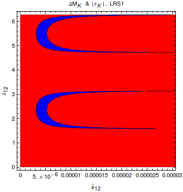
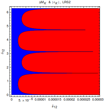
Figure 21: Ranges for $\Delta M_{K}$ (red region) and $\varepsilon_{K}$ (LRS1: left, LRS2: right) for $M_{H}=1$ TeV satisfying the bounds in Eq. (129).

 

Concerning NP contributions to $K\to\pi\nu\bar{\nu}$ decays all scalar scenarios could turn out one day to be interesting if the data on observables in $B_{s}$ and $B_{d}$ systems will show the presence of NP but negligible NP effects in $K\to\pi\nu\bar{\nu}$.

10 Flavour Violating SM $H$ Boson

We will next turn our attention to flavour violating couplings of the SM Higgs ($h$) that can be generated in the presence of other scalar particles and or new heavy vectorial fermions with $+2/3$ and $-1/3$ electric charges. In the case considered by us, new quarks with $-1/3$ charges are essential for generating flavour violating couplings to SM down-quarks but the presence of heavy quarks with $+2/3$ charges could be relevant for charm physics. Moreover, such heavy fermions could contribute to rare $K$ and $B$ decays through loop diagrams. In what follows we will not consider these loop contributions as they would lead us beyond the scope of our paper.

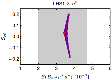
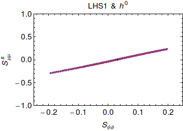
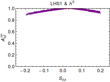
Figure 22: $S_{\psi\phi}$ versus $\overline{\mathcal{B}}(B_{s}\to\mu^{+}\mu^{-})$, $S^{s}_{\mu^{+}\mu^{-}}$ versus $S_{\psi\phi}$ and $\mathcal{A}^{\lambda}_{\Delta\Gamma}$ versus $S_{\psi\phi}$ for scalar $h^{0}$ case with $M_{h}=125~{}$GeV in LHS1. The two oases (blue and purple) overlap. Red point: SM central value.

 

The strategy and formalism developed in the previous sections can be used in a straightforward manner for the case of $h$ flavour-violating couplings to quarks. Using the general relations of Section 6 one then finds that these couplings have to be significantly smaller, by roughly an order of magnitude relatively to the corresponding couplings of a heavy scalar with a mass in the ballpark of 1 TeV. Still the presence of such contributions can remove all possible tensions within the SM in $\Delta F=2$ transitions without being in conflict with constraints from rare decays, where the SM Higgs contributions, in spite of a low Higgs mass, turn out to be small.

The reason for the smallness of SM Higgs contributions to rare decays originates from the smallness of scalar Higgs coupling to $\mu^{+}\mu^{-}$ with $\Delta^{\mu\mu}_{S}(h)=1.2\times 10^{-3}$. It is roughly a factor of 25 smaller than the largest scalar coupling allowed by $B_{s}\to\mu^{+}\mu^{-}$ for a scalar with $M_{H}=1\,{\rm TeV}$. As the correlations between $\Delta F=2$ and $\Delta F=1$ transitions in Section 6 show, this smallness of the muon couplings of SM Higgs can be compensated partly by the smallness of its mass. But it turns out that this compensation is insufficient to make the SM Higgs contributions to rare $B_{d}$ and $K$ decays relevant. We recall that these contributions do not interfere with the SM contribution from $Z$-penguins and box diagrams and are suppressed by the square of $\Delta_{S}^{\mu\mu}(h)$.

On the other hand small but visible effects in $B_{s}\to\mu^{+}\mu^{-}$ decay are still possible. We illustrate this in Figs. 22 which have been obtained using the technology developed for heavy scalars. We note that $\overline{\mathcal{B}}(B_{s}\to\mu^{+}\mu^{-})$ can be enhanced up to $8\%$ and $|S^{s}_{\mu^{+}\mu^{-}}|$ can be as large as $0.3$ but only for the maximal allowed values of $S_{\psi\phi}$.

11 Summary and Conclusions

In this paper we exhibited the pattern of flavour violation in models in which NP effects are dominated by tree-level heavy pseudoscalar (A) or scalar (H) exchanges under the assumption that the theoretical and experimental errors on various input parameters will decrease with time. In particular we have identified a number of correlations between $\Delta F=2$ and $\Delta F=1$ processes that will enable in due time to test this NP scenario. Our detailed analysis of these correlations in Section 8 shows that in the $B_{s}$ and $B_{d}$ systems a very rich pattern of NP effects is present while this is not the case in $K$ decays. This is partly opposite to $Z^{\prime}$ and $Z$ scenarios considered in [1] where the largest effects have been found in the $K$ system, even for masses of $M_{Z^{\prime}}$ outside the LHC reach.

Our results are summarized in a number of plots that have been obtained in various scenarios for the $H$ couplings and for inclusive and exclusive values of $|V_{ub}|$. We list here only few highlights:

• For each scenario we have identified allowed oases in the parameter space of the model. In each oasis particular structure of correlations between various observables will in the future either favour or exclude a given oasis.

• For the near future the correlations involving $S_{\psi K_{S}}$, $S_{\psi\phi}$ and $\mathcal{B}(B_{d}\to\mu^{+}\mu^{-})$ and $\overline{\mathcal{B}}(B_{s}\to\mu^{+}\mu^{-})$ will be the most interesting as the data on these four observables will be improved in the coming years, sharpening the outcome of our analysis and possibly ruling out some oases and scenarios of the couplings.

• Most importantly we have found that various correlations involving $S_{\psi\phi}$, $\overline{\mathcal{B}}(B_{s}\to\mu^{+}\mu^{-})$ and the CP asymmetry $S^{s}_{\mu^{+}\mu^{-}}$ show profound differences between the scenario with a pseudoscalar tree-level exchange and $Z^{\prime}$ exchange. As we explained in detail, these differences are directly related to the difference in the fundamental properties of the particles involved: their spin and CP-parity. As far as the last property is concerned also differences between the implications of the pseudoscalar and scalar exchanges have been identified. In particular the scalar contributions can only enhance $\overline{\mathcal{B}}(B_{s}\to\mu^{+}\mu^{-})$ and are invariant under the interchange of two oases in parameter space involved, which is not the case of pseudoscalar exchanges where the branching ratio can also be suppressed. The symphony of plots in Subsection 8.1, where the most important results of our paper are shown will be helpful in monitoring further developments in the measurements of the observables in question.

• Analogous comments apply to the correlations involving $S_{\psi K_{S}}$, $\mathcal{B}(B_{d}\to\mu^{+}\mu^{-})$ and the CP asymmetry $S^{d}_{\mu^{+}\mu^{-}}$ for which the symphony of plots, also presented in Subsection 8.1, is doubled in view of the dependence on the value of $|V_{ub}|$.

• We have demonstrated that the imposition of $U(2)^{3}$ symmetry on pseudoscalar and scalar quark couplings has a profound impact on the correlations in the $B_{s}$ system with much smaller effects in the $B_{d}$ system.

• We have also pointed out additional differences between $Z^{\prime}$ and pseudoscalar or scalar tree-level contributions related to channels with neutrinos in the final state, where in the $Z^{\prime}$ case these contributions could be very large but are expected to be negligible in NP scenarios considered here.

• Our short analysis of flavour-violating SM Higgs-couplings shows that in the case of rare $B_{d}$ and $K$ decays, the SM Higgs contributions are irrelevant due to the smallness of the Higgs coupling to muons after corresponding constraints from $\Delta F=2$ transitions have been taken into account. However, small but visible effects in $B_{s}\to\mu^{+}\mu^{-}$ are still allowed. On the other hand such contributions could in principle remove all tensions within $\Delta F=2$ observables observed within the SM.

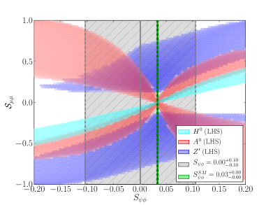
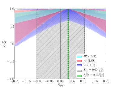
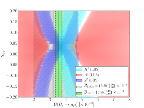
Figure 23: Overlay of the correlations for $S_{\mu\mu}^{s}$ versus $S_{\psi\phi}$ (top left), $A_{\Delta\Gamma}^{\mu\mu}$ versus $S_{\psi\phi}$ (top right) and $S_{\psi\phi}$ versus $\overline{\mathcal{B}}(B_{s}\to\mu^{+}\mu^{-})$ (bottom) for tree level scalar (cyan), pseudoscalar (red) and $Z^{\prime}$ (blue) exchange (both oases in same colour respectively) in LHS. The lepton couplings are varied in the ranges $|\Delta_{S,P}^{\mu\mu}(H)|\in[0.012,0.024]$ and $\Delta_{A}^{\mu\mu}(Z^{\prime})\in[0.3,0.7]$.

 

We close our paper by Fig. 23 in which we show the correlations involving $S_{\mu\mu}^{s}$, $S_{\psi\phi}$ and $\overline{\mathcal{B}}(B_{s}\to\mu^{+}\mu^{-})$ combining information of Fig. 8 for the tree-level scalar and pseudoscalar exchange and include also tree-level $Z^{\prime}$ exchange. The lepton couplings are not fixed but varied in the following ranges: $|\Delta_{S,P}^{\mu\mu}(H)|\in[0.012,0.024]$ and $\Delta_{A}^{\mu\mu}(Z^{\prime})\in[0.3,0.7]$. Further we do not distinguish between the two different oases here. In the $Z^{\prime}$ case we also take into account the bounds from $b\to s\ell^{+}\ell^{-}$ transitions from [8]. The patterns already identified previously and summarized above are clearly visible in these plots.

We are aware of the fact that some of the correlations presented by us would be washed out if we included all existing uncertainties. Yet, our simplified numerical analysis had as the main goal to illustrate how the decrease of theoretical, parametric and experimental uncertainties in the coming years might allow to exhibit certain features of NP, even if deviations from the SM will be only moderate. In this manner we have uncovered a world of correlations present in NP scenarios, where new effects are dominated by flavour-violating couplings of a heavy neutral pseudoscalar and scalar. In fact, within the coming years the size of the assumed uncertainties in our analysis could likely become reality not only because of improved experimental data but also improvements in theory, in particular lattice calculations of hadronic matrix elements, $B_{i}$ parameters, form factors and weak decay constants.

We are looking forward to improved experimental data and improved lattice calculations. The correlations identified in this paper will allow to monitor how simple NP scenarios discussed by us face the future precision flavour data.

Acknowledgements
We thank Robert Fleischer and Robert Ziegler for discussions. This research was financially supported by the ERC Advanced Grant project “FLAVOUR” (267104) and the Foundation for Fundamental Research on Matter (FOM). It was also partially supported by the DFG cluster of excellence “Origin and Structure of the Universe”.

References

- [1] A. J. Buras, F. De Fazio, and J. Girrbach, The Anatomy of Z’ and Z with Flavour Changing Neutral Currents in the Flavour Precision Era, JHEP 1302 (2013) 116, [arXiv:1211.1896].
- [2] M. Blanke, A. J. Buras, K. Gemmler, and T. Heidsieck, observables and in the Left-Right Asymmetric Model: Higgs particles striking back, JHEP 1203 (2012) 024, [arXiv:1111.5014].
- [3] W. Altmannshofer, A. J. Buras, S. Gori, P. Paradisi, and D. M. Straub, Anatomy and Phenomenology of FCNC and CPV Effects in SUSY Theories, Nucl.Phys. B830 (2010) 17–94, [arXiv:0909.1333].
- [4] M. Blanke et al., Rare and CP-violating and decays in the Littlest Higgs model with T-parity, JHEP 01 (2007) 066, [hep-ph/0610298].
- [5] M. Blanke, A. J. Buras, B. Duling, S. Recksiegel, and C. Tarantino, FCNC Processes in the Littlest Higgs Model with T-Parity: a 2009 Look, Acta Phys.Polon. B41 (2010) 657–683, [arXiv:0906.5454].
- [6] M. Blanke, A. J. Buras, B. Duling, K. Gemmler, and S. Gori, Rare K and B Decays in a Warped Extra Dimension with Custodial Protection, JHEP 03 (2009) 108, [arXiv:0812.3803].
- [7] W. Altmannshofer, P. Paradisi, and D. M. Straub, Model-Independent Constraints on New Physics in Transitions, JHEP 1204 (2012) 008, [arXiv:1111.1257].
- [8] W. Altmannshofer and D. M. Straub, Cornering New Physics in Transitions, JHEP 1208 (2012) 121, [arXiv:1206.0273].
- [9] A. J. Buras and J. Girrbach, On the Correlations between Flavour Observables in Minimal Models, JHEP 1301 (2013) 007, [arXiv:1206.3878].
- [10] K. De Bruyn, R. Fleischer, R. Knegjens, P. Koppenburg, M. Merk, et al., Branching Ratio Measurements of Decays, Phys.Rev. D86 (2012) 014027, [arXiv:1204.1735].
- [11] K. De Bruyn, R. Fleischer, R. Knegjens, P. Koppenburg, M. Merk, et al., Probing New Physics via the Effective Lifetime, Phys.Rev.Lett. 109 (2012) 041801, [arXiv:1204.1737].
- [12] A. J. Buras, F. De Fazio, J. Girrbach, and M. V. Carlucci, The Anatomy of Quark Flavour Observables in 331 Models in the Flavour Precision Era, JHEP 1302 (2013) 023, [arXiv:1211.1237].
- [13] A. J. Buras and L. Silvestrini, Upper bounds on and from and , Nucl. Phys. B546 (1999) 299–314, [hep-ph/9811471].
- [14] A. J. Buras, G. Colangelo, G. Isidori, A. Romanino, and L. Silvestrini, Connections between and rare kaon decays in supersymmetry, Nucl. Phys. B566 (2000) 3–32, [hep-ph/9908371].
- [15] M. Blanke, A. J. Buras, S. Recksiegel, C. Tarantino, and S. Uhlig, Correlations between and Rare Decays in the Littlest Higgs Model with T-Parity, JHEP 06 (2007) 082, [0704.3329].
- [16] D. Becirevic, N. Kosnik, F. Mescia, and E. Schneider, Complementarity of the constraints on New Physics from and from decays, Phys.Rev. D86 (2012) 034034, [arXiv:1205.5811].
- [17] A. J. Buras, R. Fleischer, J. Girrbach, and R. Knegjens, Probing New Physics with the Time-Dependent Rate, arXiv:1303.3820.
- [18] A. J. Buras, Minimal flavor violation, Acta Phys. Polon. B34 (2003) 5615–5668, [hep-ph/0310208].
- [19] A. J. Buras, S. Jager, and J. Urban, Master formulae for NLO QCD factors in the standard model and beyond, Nucl.Phys. B605 (2001) 600–624, [hep-ph/0102316].
- [20] A. J. Buras and J. Girrbach, Complete NLO QCD Corrections for Tree Level Delta F = 2 FCNC Processes, JHEP 1203 (2012) 052, [arXiv:1201.1302].
- [21] RBC and UKQCD Collaborations Collaboration, P. Boyle, N. Garron, and R. Hudspith, Neutral kaon mixing beyond the standard model with chiral fermions, Phys.Rev. D86 (2012) 054028, [arXiv:1206.5737].
- [22] V. Bertone, N. Carrasco, M. Ciuchini, P. Dimopoulos, R. Frezzotti, et al., Kaon Mixing Beyond the SM from Nf=2 tmQCD and model independent constraints from the UTA, arXiv:1207.1287.
- [23] C. Bouchard, E. Freeland, C. Bernard, A. El-Khadra, E. Gamiz, et al., Neutral mixing from flavor lattice-QCD: the Standard Model and beyond, PoS LATTICE2011 (2011) 274, [arXiv:1112.5642].
- [24] LHCb Collaboration Collaboration, G. Raven, Measurement of the CP violation phase in the system at LHCb, arXiv:1212.4140.
- [25] M. Blanke et al., Particle antiparticle mixing, , , , , and in the Littlest Higgs model with T- parity, JHEP 12 (2006) 003, [hep-ph/0605214].
- [26] S. Herrlich and U. Nierste, Enhancement of the mass difference by short distance QCD corrections beyond leading logarithms, Nucl. Phys. B419 (1994) 292–322, [hep-ph/9310311].
- [27] S. Herrlich and U. Nierste, Indirect CP violation in the neutral kaon system beyond leading logarithms, Phys. Rev. D52 (1995) 6505–6518, [hep-ph/9507262].
- [28] S. Herrlich and U. Nierste, The Complete Hamiltonian in the Next-To-Leading Order, Nucl. Phys. B476 (1996) 27–88, [hep-ph/9604330].
- [29] A. J. Buras, M. Jamin, and P. H. Weisz, Leading and next-to-leading QCD corrections to parameter and mixing in the presence of a heavy top quark, Nucl. Phys. B347 (1990) 491–536.
- [30] J. Urban, F. Krauss, U. Jentschura, and G. Soff, Next-to-leading order QCD corrections for the mixing with an extended Higgs sector, Nucl. Phys. B523 (1998) 40–58, [hep-ph/9710245].
- [31] J. Brod and M. Gorbahn, at Next-to-Next-to-Leading Order: The Charm-Top-Quark Contribution, Phys.Rev. D82 (2010) 094026, [arXiv:1007.0684].
- [32] J. Brod and M. Gorbahn, Next-to-Next-to-Leading-Order Charm-Quark Contribution to the CP Violation Parameter and , Phys.Rev.Lett. 108 (2012) 121801, [arXiv:1108.2036].
- [33] A. J. Buras and D. Guadagnoli, Correlations among new CP violating effects in observables, Phys. Rev. D78 (2008) 033005, [arXiv:0805.3887].
- [34] A. J. Buras, D. Guadagnoli, and G. Isidori, On beyond lowest order in the Operator Product Expansion, Phys.Lett. B688 (2010) 309–313, [arXiv:1002.3612].
- [35] G. Buchalla and A. J. Buras, The rare decays , and : An update, Nucl. Phys. B548 (1999) 309–327, [hep-ph/9901288].
- [36] M. Misiak and J. Urban, QCD corrections to FCNC decays mediated by Z penguins and W boxes, Phys.Lett. B451 (1999) 161–169, [hep-ph/9901278].
- [37] R. Fleischer, On Branching Ratios of Decays and the Search for New Physics in , arXiv:1208.2843.
- [38] LHCb Collaboration, G. Cowan et al., Tagged time-dependent angular analysis of decays at LHCb, LHCb-CONF-2012-002.
- [39] S. Descotes-Genon, J. Matias, and J. Virto, An analysis of mixing angles in presence of New Physics and an update of , Phys.Rev. D85 (2012) 034010, [arXiv:1111.4882].
- [40] LHCb Collaboration Collaboration, R. Aaij et al., Strong constraints on the rare decays and , Phys.Rev.Lett. 108 (2012) 231801, [arXiv:1203.4493].
- [41] LHCb Collaboration Collaboration, R. Aaij et al., First evidence for the decay , Phys.Rev.Lett. 110 (2013) 021801, [arXiv:1211.2674].
- [42] A. J. Buras, J. Girrbach, D. Guadagnoli, and G. Isidori, On the Standard Model prediction for BR(, Eur.Phys.J. C72 (2012) 2172, [arXiv:1208.0934].
- [43] R. Dowdall, C. Davies, R. Horgan, C. Monahan, and J. Shigemitsu, B-meson decay constants from improved lattice NRQCD and physical u, d, s and c sea quarks, arXiv:1302.2644.
- [44] Heavy Flavor Averaging Group Collaboration, Y. Amhis et al., Averages of B-Hadron, C-Hadron, and tau-lepton properties as of early 2012, arXiv:1207.1158.
- [45] M. Misiak, Rare -Meson Decays, arXiv:1112.5978.
- [46] M. Gorbahn and U. Haisch, Charm quark contribution to at next-to-next-to-leading order, Phys. Rev. Lett. 97 (2006) 122002, [hep-ph/0605203].
- [47] G. Isidori and R. Unterdorfer, On the short-distance constraints from , JHEP 01 (2004) 009, [hep-ph/0311084].
- [48] F. Mescia, C. Smith, and S. Trine, and : A binary star on the stage of flavor physics, JHEP 08 (2006) 088, [hep-ph/0606081].
- [49] J. Prades, ChPT Progress on Non-Leptonic and Radiative Kaon Decays, PoS KAON (2008) 022, [arXiv:0707.1789].
- [50] G. Isidori, C. Smith, and R. Unterdorfer, The rare decay within the SM, Eur. Phys. J. C36 (2004) 57–66, [hep-ph/0404127].
- [51] S. Friot, D. Greynat, and E. De Rafael, Rare kaon decays revisited, Phys. Lett. B595 (2004) 301–308, [hep-ph/0404136].
- [52] C. Bruno and J. Prades, Rare Kaon Decays in the -Expansion, Z. Phys. C57 (1993) 585–594, [hep-ph/9209231].
- [53] KTeV Collaboration, A. Alavi-Harati et al., Search for the Rare Decay , Phys. Rev. Lett. 93 (2004) 021805, [hep-ex/0309072].
- [54] KTEV Collaboration, A. Alavi-Harati et al., Search for the Decay , Phys. Rev. Lett. 84 (2000) 5279–5282, [hep-ex/0001006].
- [55] M. Bauer, S. Casagrande, U. Haisch, and M. Neubert, Flavor Physics in the Randall-Sundrum Model: II. Tree-Level Weak-Interaction Processes, JHEP 1009 (2010) 017, [arXiv:0912.1625].
- [56] M. Blanke, A. J. Buras, S. Recksiegel, and C. Tarantino, The Littlest Higgs Model with T-Parity Facing CP-Violation in Mixing, arXiv:0805.4393.
- [57] G. Buchalla, G. D’Ambrosio, and G. Isidori, Extracting short-distance physics from decays, Nucl. Phys. B672 (2003) 387–408, [hep-ph/0308008].
- [58] A. J. Buras, M. E. Lautenbacher, M. Misiak, and M. Munz, Direct CP violation in beyond leading logarithms, Nucl. Phys. B423 (1994) 349–383, [hep-ph/9402347].
- [59] E. Lunghi and A. Soni, Possible Indications of New Physics in -mixing and in Determinations, Phys. Lett. B666 (2008) 162–165, [arXiv:0803.4340].
- [60] G. Ricciardi, Brief review on semileptonic B decays, Mod.Phys.Lett. A27 (2012) 1230037, [arXiv:1209.1407].
- [61] Belle Collaboration Collaboration, I. Adachi et al., Measurement of with a hadronic tagging method using the full data sample of belle, arXiv:1208.4678.
- [62] C. Tarantino, Flavor Lattice QCD in the Precision Era, arXiv:1210.0474.
- [63] A. J. Buras, J. Girrbach, and R. Ziegler, Particle-Antiparticle Mixing, CP Violation and Rare K and B Decays in a Minimal Theory of Fermion Masses, JHEP 1304 (2013) 168, [arXiv:1301.5498].
- [64] I. de Medeiros Varzielas, C. Hambrock, G. Hiller, M. Jung, P. Leser, et al., Proceedings of the 2nd Workshop on Flavor Symmetries and Consequences in Accelerators and Cosmology (FLASY12), arXiv:1210.6239.
- [65] M. Antonelli, D. M. Asner, D. A. Bauer, T. G. Becher, M. Beneke, et al., Flavor Physics in the Quark Sector, Phys.Rept. 494 (2010) 197–414, [arXiv:0907.5386].
- [66] LHCb Collaboration Collaboration, R. Aaij et al., Implications of LHCb measurements and future prospects, EPJ C 73 (2013) 2373, [arXiv:1208.3355].
- [67] Particle Data Group Collaboration, K. Nakamura et al., Review of particle physics, J.Phys.G G37 (2010) 075021.
- [68] J. Laiho, E. Lunghi, and R. S. Van de Water, Lattice QCD inputs to the CKM unitarity triangle analysis, Phys. Rev. D81 (2010) 034503, [arXiv:0910.2928]. Updates available on http://latticeaverages.org/.
- [69] K. Chetyrkin, J. Kuhn, A. Maier, P. Maierhofer, P. Marquard, et al., Charm and Bottom Quark Masses: An Update, Phys.Rev. D80 (2009) 074010, [arXiv:0907.2110].
- [70] HPQCD Collaboration Collaboration, I. Allison et al., High-Precision Charm-Quark Mass from Current-Current Correlators in Lattice and Continuum QCD, Phys.Rev. D78 (2008) 054513, [arXiv:0805.2999].
- [71] CDF Collaboration, D0 Collaboration Collaboration, T. Aaltonen et al., Combination of the top-quark mass measurements from the Tevatron collider, Phys.Rev. D86 (2012) 092003, [arXiv:1207.1069].
- [72] Particle Data Group Collaboration, J. Beringer et al., Review of Particle Physics (RPP), Phys.Rev. D86 (2012) 010001.
- [73] A. J. Buras and J. Girrbach, BSM models facing the recent LHCb data: A First look, Acta Phys.Polon. B43 (2012) 1427, [arXiv:1204.5064].
- [74] R. Barbieri, G. Isidori, J. Jones-Perez, P. Lodone, and D. M. Straub, U(2) and Minimal Flavour Violation in Supersymmetry, Eur.Phys.J. C71 (2011) 1725, [arXiv:1105.2296].
- [75] R. Barbieri, P. Campli, G. Isidori, F. Sala, and D. M. Straub, B-decay CP-asymmetries in SUSY with a flavour symmetry, Eur.Phys.J. C71 (2011) 1812, [arXiv:1108.5125].
- [76] R. Barbieri, D. Buttazzo, F. Sala, and D. M. Straub, Flavour physics from an approximate symmetry, JHEP 1207 (2012) 181, [arXiv:1203.4218].
- [77] R. Barbieri, D. Buttazzo, F. Sala, and D. M. Straub, Less Minimal Flavour Violation, JHEP 1210 (2012) 040, [arXiv:1206.1327].
- [78] A. Crivellin, L. Hofer, and U. Nierste, The MSSM with a Softly Broken Flavor Symmetry, PoS EPS-HEP2011 (2011) 145, [arXiv:1111.0246].
- [79] A. Crivellin, L. Hofer, U. Nierste, and D. Scherer, Phenomenological consequences of radiative flavor violation in the MSSM, Phys.Rev. D84 (2011) 035030, [arXiv:1105.2818].
- [80] A. Crivellin and U. Nierste, Supersymmetric renormalisation of the CKM matrix and new constraints on the squark mass matrices, Phys.Rev. D79 (2009) 035018, [arXiv:0810.1613].
- [81] A. J. Buras, M. V. Carlucci, S. Gori, and G. Isidori, Higgs-mediated FCNCs: Natural Flavour Conservation vs. Minimal Flavour Violation, JHEP 1010 (2010) 009, [arXiv:1005.5310].