Entanglement Classification of extended Greenberger-Horne-Zeilinger-Symmetric States

Abstract

In this paper we analyze entanglement classification of extended Greenberger-Horne-Zeilinger-symmetric states $\rho^{ES}$, which is parametrized by four real parameters $x$, $y_{1}$, $y_{2}$ and $y_{3}$. The condition for separable states of $\rho^{ES}$ is analytically derived. The higher classes such as bi-separable, W, and Greenberger-Horne-Zeilinger classes are roughly classified by making use of the class-specific optimal witnesses or map from the extended Greenberger-Horne-Zeilinger symmetry to the Greenberger-Horne-Zeilinger symmetry. From this analysis we guess that the entanglement classes of $\rho^{ES}$ are not dependent on $y_{j}\hskip 5.69046pt(j=1,2,3)$ individually, but dependent on $y_{1}+y_{2}+y_{3}$ collectively. The difficulty arising in extension of analysis with Greenberger-Horne-Zeilinger symmetry to the higher-qubit system is discussed.

I Introduction

Entanglementhorodecki09 is an important physical resource in the context of quantum information theoriestext . As shown for last two decades it plays a crucial role in quantum teleportationteleportation , superdense codingsuperdense , quantum cloningclon , quantum cryptographycryptography . It is also quantum entanglement, which makes the quantum computer outperform the classical onecomputer . Therefore, it is greatly important task to understand what kind and how much entanglement a given quantum state has.

For multipartite quantum states there are several types of entanglement. Each type is in general categorized by stochastic local operations and classical communication (SLOCC)bennet00 . Thus, these types of entanglement is often called SLOCC-equivalence classes. For example, for three-qubit pure statesdur00 there are six SLOCC-equivalence classes such as separable, three bi-separable ($A-BC$, $B-AC$, $C-AB$), W and Greenberger-Horne-Zeilinger (GHZ) classes. Among them genuine tripartite entanglement arises in W and GHZ classes. The representative states of these classes are

$$\lvert\mbox{GHZ}\rangle=\frac{1}{\sqrt{2}}\left[\lvert 000\rangle+\lvert 111\rangle\right]$$ (1)

$$\lvert\mbox{W}\rangle=\frac{1}{\sqrt{3}}\left[\lvert 001\rangle+\lvert 010\rangle+\lvert 100\rangle\right].$$

One of the most remarkable fact in this classification is that the set of W states forms measure zero in the whole three-qubit pure states.

This classification can be extended to three-qubit mixed statesthreeM . Following Ref.threeM the whole three-qubit mixed states are classified as separable (S), bi-separable (B), W and GHZ classes. These classes satisfy a linear hierarchy S $\subset$ B $\subset$ W $\subset$ GHZ. One remarkable fact, which was proved in this reference, is that the W-class is not of measure zero among all mixed-states.

Although SLOCC classes for three-qubit system are well-known, we still do not know how the entanglement is classified in multi-qubit system except four-qubit pure states, where there are nine SLOCC classesfourP . Furthermore, still it is very difficult problem to find a SLOCC class of a given three-qubit mixed state except few rare cases. Thus, it is important task to develop a method, which enables us to find a SLOCC class of an arbitrary three-qubit states.

Recently, a significant progress is made in this issue. In Ref.elts12-1 a complete SLOCC classification for the set of the GHZ-symmetric states was reported (see Fig. 1). According to this complete classification the ratio of number of S, B, W, and GHZ states in the whole set of the GHZ-symmetric states is $1:1:1.076:0.924$. Thus, W class is not of measure zero in this restricted set of the three-qubit states. Using this classification the three-tangle $\tau$ for the arbitrary GHZ-symmetric states is explored in Ref.siewert12-1 . Moreover, this complete classification is used to construct the class-specific optimal witnesses for the three-qubit entanglementelts12-2 .

The purpose of this paper is to explore a possible extension of Ref.elts12-1 to treat more three-qubit mixed states. For this purpose we enlarge the symmetry group to, so-called, the extended GHZ symmetry group. The whole set of quantum states invariant under the extended GHZ symmetry group is parametrized by four real parameters $(x,y_{1},y_{2},y_{3})$. The complete classification for S states is analytically derived. However, the classification for B, W, and GHZ states is incomplete. Rough classification for B, W, and GHZ states is explored by making use of the class-specific optimal witnesseselts12-2 or GHZ symmetryelts12-1 , respectively.

The paper is organized as follows. In next section we review Ref. elts12-1 briefly. In section III we discuss on the extended GHZ symmetry. It is found that the set of extended GHZ-symmetric states is parametrized by four real parameters. In section IV we derive a condition for the separable region in the four-dimensional parameter space by applying a Lagrange multiplier method. In section V we perform a entanglement classification of the extended GHZ-symmetric states roughly by making use of the class-specific optimal witnesses or map from extended GHZ symmetry to GHZ symmetry. In section VI a conclusion is given. In particular, we discuss on the difficulty arising when we extend the analysis with the GHZ symmetry to the higher-qubit systems in this section.

II classification of GHZ-symmetric states

In this section we review Ref. elts12-1 briefly. The GHZ-symmetric states are the three-qubit states which are invariant under the following transformations: (i) qubit permutations, (ii) simultaneous three-qubit flips (i.e., application of $\sigma_{x}\otimes\sigma_{x}\otimes\sigma_{x}$), (iii) qubit rotations about the $z$-axis of the form

$$U(\phi_{1},\phi_{2})=e^{i\phi_{1}\sigma_{z}}\otimes e^{i\phi_{2}\sigma_{z}}\otimes e^{-i(\phi_{1}+\phi_{2})\sigma_{z}}.$$ (2)

It is straightforward to show that the general form of the GHZ-symmetric states $\rho^{S}$ is parametrized by two real parameters $x$ and $y$ as

$$\rho^{S}(x,y)=\left(x+\frac{\sqrt{3}}{2}y+\frac{1}{8}\right)\lvert\mbox{GHZ}_{+}\rangle\langle\mbox{GHZ}_{+}\lvert+\left(-x+\frac{\sqrt{3}}{2}y+\frac{1}{8}\right)\lvert\mbox{GHZ}_{-}\rangle\langle\mbox{GHZ}_{-}\lvert$$ (3)

$$+\left(\frac{1}{8}-\frac{y}{2\sqrt{3}}\right)\bigg{[}\lvert 001\rangle\langle 001\lvert+\lvert 010\rangle\langle 010\lvert+\lvert 011\rangle\langle 011\lvert+\lvert 100\rangle\langle 100\lvert+\lvert 101\rangle\langle 101\lvert+\lvert 110\rangle\langle 110\lvert\bigg{]}$$

where

$$\lvert\mbox{GHZ}_{\pm}\rangle=\frac{1}{\sqrt{2}}\left(\lvert 000\rangle\pm\lvert 111\rangle\right).$$ (4)

The real parameters $x$ and $y$ are introduced such that the Euclidean metric in the $(x,y)$ plane coincides with the Hilbert-Schmidt metric $d(A,B)^{2}\equiv\frac{1}{2}\mbox{tr}(A-B)^{\dagger}(A-B)$, i.e.,

$$d^{2}\left(\rho^{S}(x_{1},y_{1}),\rho^{S}(x_{2},y_{2})\right)=(x_{2}-x_{1})^{2}+(y_{2}-y_{1})^{2}.$$ (5)

Since $\rho^{S}(x,y)$ is a quantum state, the parameters $x$ and $y$ are restricted as

$$-\frac{1}{4\sqrt{3}}\leq y\leq\frac{\sqrt{3}}{4},\hskip 28.45274pty\geq\pm\frac{2}{\sqrt{3}}x-\frac{1}{4\sqrt{3}}.$$ (6)

This restriction can be easily derived by computing the eigenvalues of $\rho^{S}$. Thus, the set of the GHZ-symmetric states are represented as a triangle in $(x,y)$ plane as Fig. 1 shows. Each point inside the triangle corresponds to each GHZ-symmetric state.

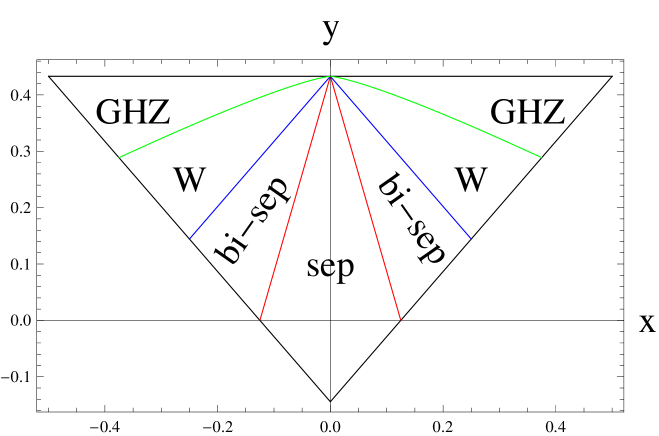
Figure 1: Complete classification of GHZ-symmetric states.

In order to classify the GHZ-symmetric states it is worthwhile noting that there exists a map from an arbitrary three-qubit pure state $\lvert\psi\rangle$ to the GHZ-symmetric state $\rho^{S}(\psi)$, which is defined as

$$\rho^{S}(\psi)=\int dUU\lvert\psi\rangle\langle\psi\lvert U^{\dagger},$$ (7)

where the integral is understood to cover the entire GHZ symmetry group. If, for example, $\lvert\psi\rangle=\sum_{i,j,k=0}^{1}\psi_{ijk}\lvert ijk\rangle$, the corresponding $\rho^{S}(\psi)$ is given by Eq. (3) with

$$x=\frac{1}{2}\left(\psi_{000}^{*}\psi_{111}+\psi_{000}\psi_{111}^{*}\right)\hskip 28.45274pty=\frac{1}{\sqrt{3}}\left(|\psi_{000}|^{2}+|\psi_{111}|^{2}-\frac{1}{4}\right).$$ (8)

Another fact we will use for classification is that applying $GL(2,\mathbb{C})$ transformations to any qubit does not change the entanglement class of a multiqubit state. This fact leads from the invariance of the entanglement class under the stochastic local operations and classical communication (SLOCC)dur00 ; bennet00 .

In order to find the boundary of each entanglement class, therefore, we fix the $y$ coordinate and derive the maximum of $|x|$ by using Eq. (8) and applying the Lagrange multiplier method. Since mirror symmetry implies $x_{min}=-x_{max}$, it is possible to restrict ourselves to $x\geq 0$. This procedure yields some region in the $(x,y)$ plane. If this region is a convex, the set of states corresponding to this region exhibits a same entanglement property. If it is not convex, the proper boundary of the class is obtained by the convex hull of this region.

The entanglement classification derived in this way is summarized in Fig. 1. Recently, this classification was used to compute the three-tangleckw of the entire GHZ-symmetric states analyticallysiewert12-1 . More recently, this is used to derive the class-specific optimal witnesses for three-qubit entanglementelts12-2 .

III Extended GHZ symmetry

In this section we will relax the condition of the GHZ symmetry to treat more large set of the three-qubit states. The symmetry we consider is identical with the GHZ symmetry without first condition, i.e., qubit permutations. We will call this the extended GHZ symmetry.

It is not difficult to show that the general form of the extended GHZ-symmetric states is parametrized by four real parameters $x$, $y_{1}$, $y_{2}$, and $y_{3}$ as

$$\rho^{ES}(x,y_{1},y_{2},y_{3})$$ (9)

$$=\left(\frac{1}{8}+\frac{y_{1}+y_{2}+y_{3}}{2}+x\right)\lvert GHZ_{+}\rangle\langle GHZ_{+}\lvert+\left(\frac{1}{8}+\frac{y_{1}+y_{2}+y_{3}}{2}-x\right)\lvert GHZ_{-}\rangle\langle GHZ_{-}\lvert$$

$$+\left(\frac{1}{8}-\frac{y_{1}+y_{2}-y_{3}}{2}\right)\bigg{[}\lvert 001\rangle\langle 001\lvert+\lvert 110\rangle\langle 110\lvert\bigg{]}+\left(\frac{1}{8}-\frac{y_{1}-y_{2}+y_{3}}{2}\right)\bigg{[}\lvert 010\rangle\langle 010\lvert+\lvert 101\rangle\langle 101\lvert\bigg{]}$$

$$+\left(\frac{1}{8}-\frac{-y_{1}+y_{2}+y_{3}}{2}\right)\bigg{[}\lvert 011\rangle\langle 011\lvert+\lvert 100\rangle\langle 100\lvert\bigg{]}.$$

The parameters are chosen so that the four-dimensional Euclidean metric coincides with the Hilbert-Schmidt metric, i.e.,

$$d^{2}\bigg{(}\rho^{ES}(\bar{x},\bar{y}_{1},\bar{y}_{2},\bar{y}_{3}),\rho^{ES}(x,y_{1},y_{2},y_{3})\bigg{)}=(\bar{x}-x)^{2}+(\bar{y}_{1}-y_{1})^{2}+(\bar{y}_{2}-y_{2})^{2}+(\bar{y}_{3}-y_{3})^{2}.$$ (10)

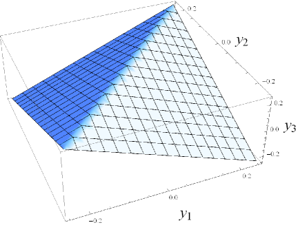
Figure 2: Pictorial representation of Eq. (11). Unlike the GHZ-symmetric case each point inside the triangle in (b) corresponds to infinite number of quantum states with same $y_{1}+y_{2}+y_{3}$.

Since $\rho^{ES}$ should be a physical state, the parameters are restricted as

$$|y_{1}+y_{2}|-\frac{1}{4}\leq y_{3}\leq\frac{1}{4}-|y_{1}-y_{2}|,\hskip 28.45274pt0\leq\frac{1}{8}+\frac{y_{1}+y_{2}+y_{3}}{2}\pm x\leq 1.$$ (11)

The restriction (11) can be depicted pictorially. As Fig. 2(a) shows, the physically available value of $y_{i}\hskip 2.84544pt(i=1,2,3)$ is confined inside polyhedron in the three-dimensional $(y_{1},y_{2},y_{3})$ space. As this figure exhibits, $y_{i}$’s are restricted by $-\frac{1}{4}\leq y_{1},y_{2},y_{3}\leq\frac{1}{4}$. However, as Fig. 2(b) shows, $y_{1}+y_{2}+y_{3}$ is restricted by $-\frac{1}{4}\leq y_{1}+y_{2}+y_{3}\leq\frac{3}{4}$ depending on $x$. Unlike the GHZ-symmetric case each point inside the triangle in Fig. 2(b) corresponds to infinite number of quantum states with same $y_{1}+y_{2}+y_{3}$.

Similarly to GHZ symmetry there exists a mapping from a set of the three-qubit pure states to the set of the extended GHZ-symmetric states. Let $\lvert\psi\rangle$ be an arbitrary three-qubit pure state. Then, the corresponding extended GHZ-symmetric state is given by Eq. (7). The only difference is a change of the symmetry group from the GHZ symmetry to the extended GHZ symmetry. If, for example, $\lvert\psi\rangle=\sum_{i,j,k=0}^{1}\psi_{ijk}\lvert ijk\rangle$, the corresponding $\rho^{ES}(\psi)$ is given by Eq.(9) with

$$x=\frac{1}{2}\left(\psi_{000}\psi_{111}^{*}+\psi_{000}^{*}\psi_{111}\right)$$ (12)

$$y_{1}=\frac{1}{2}\left(|\psi_{000}|^{2}+|\psi_{111}|^{2}+|\psi_{011}|^{2}+|\psi_{100}|^{2}\right)-\frac{1}{4}$$

$$y_{2}=\frac{1}{2}\left(|\psi_{000}|^{2}+|\psi_{111}|^{2}+|\psi_{101}|^{2}+|\psi_{010}|^{2}\right)-\frac{1}{4}$$

$$y_{3}=\frac{1}{2}\left(|\psi_{000}|^{2}+|\psi_{111}|^{2}+|\psi_{110}|^{2}+|\psi_{001}|^{2}\right)-\frac{1}{4}.$$

It is worthwhile noting a relation

$$(u\otimes u\otimes u)\rho^{ES}(x,y_{1},y_{2},y_{3})(u\otimes u\otimes u)^{\dagger}=\rho^{ES}(-x,y_{1},y_{2},y_{3})$$ (13)

where $u=\left(\begin{array}[]{cc}0&1\\ -1&0\end{array}\right)$. This implies that the sign of $x$ does not change the entanglement class of $\rho^{ES}(x,y_{1},y_{2},y_{3})$. Therefore, it is convenient to restrict ourselves to $x\geq 0$ in the following.

IV Separable states

In this section we will find a region in the four-dimensional $(x,y_{1},y_{2},y_{3})$ space, where the separable states reside. The calculation procedure is similar to Ref.elts12-1 . First, we define a general form of the fully separable three-qubit pure state by making use of the local-unitary transformation, i.e., $\lvert\psi^{sep}\rangle=\left(U_{1}\otimes U_{2}\otimes U_{3}\right)\lvert 000\rangle$, where

$$U_{j}=\left(\begin{array}[]{cc}A_{j}&-B_{j}^{*}\\ B_{j}&A_{j}^{*}\end{array}\right)\hskip 28.45274pt|B_{j}|^{2}=1-|A_{j}|^{2}.$$ (14)

Second, we map $\lvert\psi^{sep}\rangle$ to the extend GHZ-symmetric state $\rho^{ES}(\psi^{sep})$ by using a map discussed in the previous section. Finally, we maximize $x$ when $y_{1}$, $y_{2}$, and $y_{3}$ are fixed.

Combining Eq. (12) and Eq. (14), $\rho^{ES}(\psi^{sep})$ is given by Eq. (9) with

$$x=|A_{1}||A_{2}||A_{3}|\sqrt{1-|A_{1}|^{2}}\sqrt{1-|A_{2}|^{2}}\sqrt{1-|A_{3}|^{2}}$$ (15)

$$\mu_{1}=|A_{2}|^{2}|A_{3}|^{2}+(1-|A_{2}|^{2})(1-|A_{3}|^{2})$$

$$\mu_{2}=|A_{1}|^{2}|A_{3}|^{2}+(1-|A_{1}|^{2})(1-|A_{3}|^{2})$$

$$\mu_{3}=|A_{1}|^{2}|A_{2}|^{2}+(1-|A_{1}|^{2})(1-|A_{2}|^{2}),$$

where $\mu_{i}=2y_{i}+\frac{1}{2}$. In order to apply the Lagrange multiplier method we define

$$x^{\Lambda}=x+\sum_{i=1}^{3}\Lambda_{i}\Theta_{i},$$ (16)

where $\Lambda_{i}$’s are the Lagrange multiplier constants and $\Theta_{i}$’s are the constraints given by

$$\Theta_{1}=|A_{2}|^{2}|A_{3}|^{2}+(1-|A_{2}|^{2})(1-|A_{3}|^{2})-\mu_{1}$$ (17)

$$\Theta_{2}=|A_{1}|^{2}|A_{3}|^{2}+(1-|A_{1}|^{2})(1-|A_{3}|^{2})-\mu_{2}$$

$$\Theta_{3}=|A_{1}|^{2}|A_{2}|^{2}+(1-|A_{1}|^{2})(1-|A_{2}|^{2})-\mu_{3}.$$

Before proceeding further, it is worthwhile to compare Eq. (16) with the corresponding equation derived for GHZ-symmetric case at this stage. For GHZ-symmetric caseelts12-1 $x^{\Lambda}$ for the separable states becomes

$$x^{\Lambda}=|A_{1}||A_{2}||A_{3}|\sqrt{1-|A_{1}|^{2}}\sqrt{1-|A_{2}|^{2}}\sqrt{1-|A_{3}|^{2}}+\Lambda\Theta$$ (18)

$$\Theta=|A_{1}|^{2}|A_{2}|^{2}|A_{3}|^{2}+(1-|A_{1}|^{2})(1-|A_{2}|^{2})(1-|A_{3}|^{2})-\left(\sqrt{3}y+\frac{1}{4}\right).$$

Thus $x^{\Lambda}$ in Eq. (18) has a $A_{i}\leftrightarrow A_{j}$ symmetry. Thus, the maximum of $x$ occurs when $|A_{1}|=|A_{2}|=|A_{3}|$, which drastically simplifies the calculation. However, as Eq. (16) and Eq. (17) show, $x^{\Lambda}$ in Eq. (16) does not have this symmetry. This is due to the fact that the extended GHZ symmetry is less symmetric than the GHZ symmetry.

The Lagrange multiplier method generates three equations $\frac{\partial x^{\Lambda}}{\partial|A_{i}|}=0\hskip 5.69046pt(i=1,2,3)$. Since we have three Lagrange multiplier constants, these equations can be used to express $\Lambda_{i}$ in terms of $|A_{i}|$. Thus, we should determine $|A_{i}|$ from only three constraints $\Theta_{i}=0$, which yields

$$|A_{1}|^{2}=\frac{y_{1}\pm 2\sqrt{y_{1}y_{2}y_{3}}}{2y_{1}}\hskip 28.45274pt|A_{2}|^{2}=\frac{y_{2}\pm 2\sqrt{y_{1}y_{2}y_{3}}}{2y_{2}}\hskip 28.45274pt|A_{3}|^{2}=\frac{y_{3}\pm 2\sqrt{y_{1}y_{2}y_{3}}}{2y_{3}}.$$ (19)

Therefore, $|A_{1}|=|A_{2}|=|A_{3}|$ doe not hold unless $y_{1}=y_{2}=y_{3}$. This is due to the less-symmetric nature of the extended GHZ symmetry compared to the GHZ symmetry. From Eq. (19) $x_{max}$ is given by

$$x_{max}=\frac{1}{8}\sqrt{\frac{(y_{1}-4y_{2}y_{3})(y_{2}-4y_{1}y_{3})(y_{3}-4y_{1}y_{2})}{y_{1}y_{2}y_{3}}}.$$ (20)

Eq. (20) gives a certain boundary in the four-dimensional $(x,y_{1},y_{2},y_{3})$ space, inside of which the extended GHZ-symmetric separable states reside. It is worthwhile noting two points at the present stage. First, if the term inside the square root in r.h.s. of Eq. (20) is negative at some point (or region) inside the polyhedron of Fig. 2(a), this means that this point is excluded from the boundary. This is similar to $-\frac{1}{4\sqrt{3}}\leq y<0$ region in the GHZ-symmetric case as Fig. 1 exhibits. Second, if the region generated by Eq. (20) is not convex, we should extend it to its convex hull because the set of each entanglement class should be convex set.

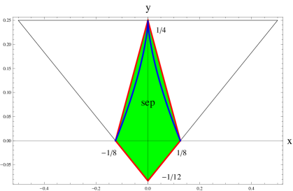
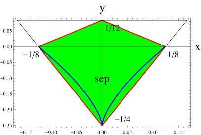
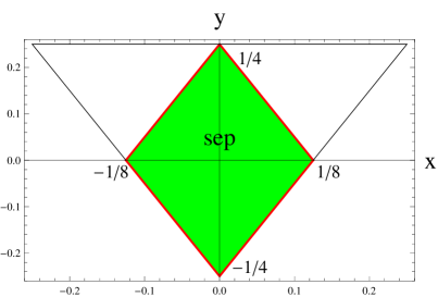
Figure 3: Separable region for (a) $y_{1}=y_{2}=y_{3}\equiv y$, (b) $y_{1}=y_{2}=-y_{3}\equiv y$, (c) $y_{1}=y_{2}=0$ and $y_{3}\equiv y$. For first two cases Eq. (20) generates concave regions (see blue lines). Thus the convex hull (red line) for each case is chosen as a separable region. For last case, however, Eq. (20) generates a convex separable region (see red line). If $y_{1}=-y_{2}=-y_{3}\equiv y$, the separable region in the $(x,y)$ plane becomes the same with (b) upside down.

Now, we consider several special cases. If $y_{1}=y_{2}=y_{3}\equiv y$, Eq. (11) gives $-\frac{1}{12}\leq y\leq\frac{1}{4}$ and $x_{max}$ becomes

$$x_{max}=\frac{1}{8}(1-4y)^{3/2}.$$ (21)

Since this is not convex (see blue line of Fig. 3(a)), we have to choose a convex hull, which is

$$x_{max}=\frac{1}{8}-\frac{y}{2}.$$ (22)

This region is depicted in Fig. 3(a) as a green color.

As a second example, let us consider a case of $y_{1}=y_{2}=-y_{3}\equiv y$. In this case Eq. (11) gives $-\frac{1}{4}\leq y\leq\frac{1}{12}$. Then, from Eq. (20) $x_{max}$ reduces to

$$x_{max}=\frac{1}{8}(1+4y)^{3/2}.$$ (23)

Since this is not convex (see blue line of Fig. 3(b)) and it is evident that the states with $x=0$ are separable, we should choose a separable region as a green color region in Fig. 3(b). If $y_{1}=-y_{2}=-y_{3}\equiv y$, the separable region in the $(x,y)$ plane becomes the same with Fig. 3(b) upside down.

As a third example, let us consider a case of $(y_{1},y_{2},y_{3})=(0,0,y)$. In this case Eq. (11) gives $-\frac{1}{4}\leq y\leq\frac{1}{4}$ and Eq. (20) yields

$$x_{max}=\frac{1}{8}(1-4y).$$ (24)

The corresponding separable region is plotted in Fig. 3(c) as a green color. Since it is convex, we do not need to choose a convex hull in this case.

Finally, let us consider the positive partial transpose (PPT) states in the extended GHZ-symmetric states $\rho^{ES}(x,y_{1},y_{2},y_{3})$. Taking a partial transposition over the first qubit and computing the eigenvalues of the resulting matrix, one can derive the PPT condition for positive $x$ as $x\leq\alpha_{4}$, where

$$\alpha_{2}=\frac{1}{8}-\frac{y_{1}+y_{2}-y_{3}}{2},\hskip 28.45274pt\alpha_{3}=\frac{1}{8}-\frac{y_{1}-y_{2}+y_{3}}{2},\hskip 28.45274pt\alpha_{4}=\frac{1}{8}-\frac{-y_{1}+y_{2}+y_{3}}{2}.$$ (25)

Performing similar calculation for second and third qubits, it is straightforward to derive a PPT condition of $\rho^{ES}(x,y_{1},y_{2},y_{3})$ as

$$x\leq x_{max}=\min(\alpha_{2},\alpha_{3},\alpha_{4}).$$ (26)

One can show that the separable regions in Fig. 3 exactly coincide with the region, where the PPT condition (26) holds.

V Rough Classification using the class-specific optimal witness operators

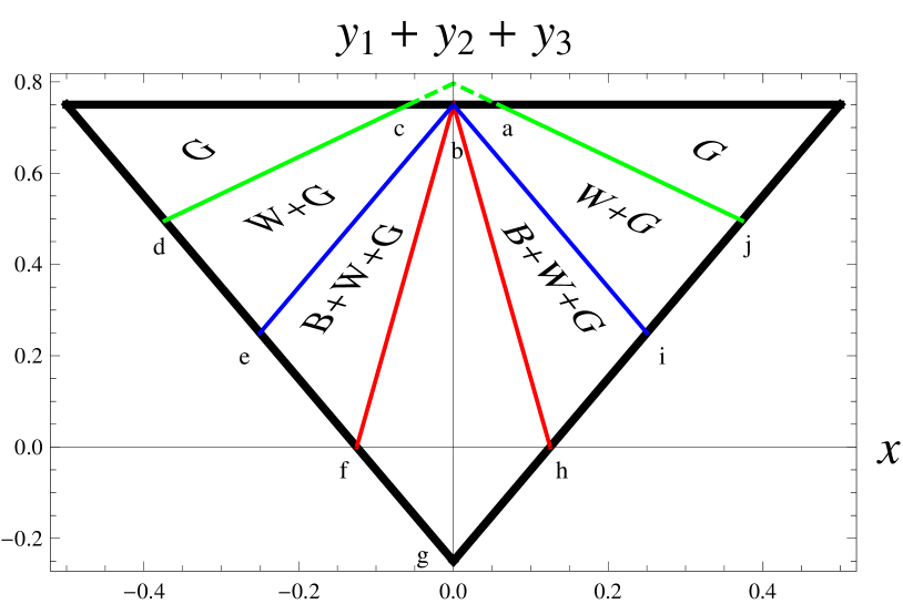
Figure 4: Rough SLOCC classification of the extended GHZ-symmetric states $\rho^{ES}$ given in Eq. (9). G, W, and B stand for GHZ class, W class, and bi-separable class. The symbol ‘+’ means coexistence. For example, W+G means the coexistence of GHZ and W classes.

The Lagrange multiplier method used in the previous section to derive the region for the separable states cannot be used to derive the region for the bi-separable states. The reason is as follows. If we choose first qubit as a separable qubit such as $\lvert\psi^{bisep}\rangle=(G_{1}\otimes G_{2}\otimes G_{3})\lvert 0\rangle\otimes\frac{1}{\sqrt{2}}(\lvert 00\rangle+\lvert 11\rangle)$, where

$$G_{j}=\left(\begin{array}[]{cc}A_{j}&B_{j}\\ C_{j}&D_{j}\end{array}\right),$$ (29)

the mapping from a set of the three-qubit pure states to the set of the extended GHZ-symmetric states cannot change the separability of the first qubit because the qubit permutation is not involved in the extended GHZ symmetry. Since, however, the definition of the bi-separable mixed state means a quantum state whose pure-states ensemble can be represented as only separable and bi-separable states without restriction to the separable qubit, the Lagrange multiplier method used in the previous section cannot be applied for deriving the region for the bi-separable extended GHZ-symmetric states.

In this paper, instead of the Lagrange multiplier method, we use the class-specific optimal witness operators

$$\mathcal{W}_{\mathrm{bisep\setminus sep}}=\openone-4\lvert\mathrm{GHZ}_{+}\rangle\!\langle\mathrm{GHZ}_{+}\lvert+2\lvert\mathrm{GHZ}_{-}\rangle\!\langle\mathrm{GHZ}_{-}\lvert$$ (30)

$$\mathcal{W}_{W\setminus\mathrm{bisep}}=\frac{1}{2}\openone-\lvert\mathrm{GHZ}_{+}\rangle\!\langle\mathrm{GHZ}_{+}\lvert$$

$$\mathcal{W}_{\mathrm{GHZ}\setminus W}(v_{0})=\frac{3}{4}\openone-\frac{3}{v_{0}^{2}-2v_{0}+4}\ \lvert\mathrm{GHZ}_{+}\rangle\!\langle\mathrm{GHZ}_{+}\lvert-\frac{3}{v_{0}^{2}+2v_{0}+4}\ \lvert\mathrm{GHZ}_{-}\rangle\!\langle\mathrm{GHZ}_{-}\lvert,$$

which are derived in Ref.elts12-2 by using the classification of the GHZ-symmetric states. Here, we choose $v_{0}=0.981$, which corresponds to the fact that the optimal witness operators yield an exact classification to the Werner state

$$\rho^{W}=p\lvert\mathrm{GHZ}_{+}\rangle\!\langle\mathrm{GHZ}_{+}\lvert+(1-p)\frac{1}{8}\openone.$$ (31)

The information the class-specific witness $\mathcal{W}_{\mathrm{A\setminus B}}$ provides is as follows. Let $\rho$ be an arbitrary three-qubit quantum state. If $\mbox{tr}(\mathcal{W}_{\mathrm{A\setminus B}}\rho)<0$, this means that $\rho$ is in A or its higher class in the three-qubit hierarchy S $\subset$ B $\subset$ W $\subset$ GHZ.

Using Eq. (30) and Eq. (9) it is straightforward to show

$$\mbox{tr}\left[\mathcal{W}_{\mathrm{bisep\setminus sep}}\rho^{ES}\right]=\frac{3}{4}-(y_{1}+y_{2}+y_{3})-6x$$ (32)

$$\mbox{tr}\left[\mathcal{W}_{\mathrm{W\setminus bisep}}\rho^{ES}\right]=\frac{1}{2}\left[\frac{3}{4}-(y_{1}+y_{2}+y_{3})-2x\right]$$

$$\mbox{tr}\left[\mathcal{W}_{\mathrm{GHZ\setminus W}}\rho^{ES}\right]$$

$$=\frac{3(v_{0}^{2}+4)}{(v_{0}^{2}-2v_{0}+4)(v_{0}^{2}+2v_{0}+4)}\left[\frac{(v_{0}^{2}+3)(v_{0}^{2}+4)-4v_{0}^{2}}{4(v_{0}^{2}+4)}-(y_{1}+y_{2}+y_{3})-\frac{4}{v_{0}^{2}+4}x\right].$$

It is worthwhile noting that Eq. (32) is not dependent on $y_{j}\hskip 5.69046pt(j=1,2,3)$ individually, but dependent on $y_{1}+y_{2}+y_{3}$. The information we can gain from Eq. (32) is as follows. The extended GHZ-symmetric separable states should be confined in a polygon $(b,f,g,h)$ in Fig. 4. The extended GHZ-symmetric bi-separable states should be confined in a polygon $(b,e,g,i)$. The extended GHZ-symmetric W states should be confined in a polygon $(a,c,d,g,j)$. Of course, all SLOCC classes should be distributed with obeying the three-qubit hierarchy S $\subset$ B $\subset$ W $\subset$ GHZ. This information is pictorially depicted in Fig. 4. The three examples discussed in the previous section can be shown to be consistent with this information, i.e., all green regions in Fig. 3 are contained in the polygon $(b,f,g,h)$.

There is another way, which enables us to get a rough classification of the extended GHZ-symmetric states $\rho^{ES}$. First, we map from $\rho^{ES}$ in Eq. (9) to $\rho^{S}$ in Eq. (3), which results in $\rho^{S}(\rho^{ES})$. Then, the parameters $x$ and $y$ of $\rho^{S}(\rho^{ES})$ are

$$x=\frac{1}{2}\left(\rho_{000,111}^{ES}+\rho_{111,000}^{ES}\right)=x$$ (33)

$$y=\frac{1}{\sqrt{3}}\left(\rho_{000,000}^{ES}+\rho_{111,111}^{ES}-\frac{1}{4}\right)=\frac{1}{\sqrt{3}}(y_{1}+y_{2}+y_{3}).$$

Since $\rho^{S}(\rho^{ES})$ should be lower class than $\rho^{ES}$, we conclude

(i) $\rho^{ES}$ is a GHZ class if $\rho^{S}(\rho^{ES})$ is a GHZ class

(ii) $\rho^{ES}$ is a GHZ or W class if $\rho^{S}(\rho^{ES})$ is a W class

(iii) $\rho^{ES}$ is a GHZ, W, or B class if $\rho^{S}(\rho^{ES})$ is a B class.

This makes a similar (but not exactly same) figure to Fig. 4.

VI Conclusion

In this paper we analyze the SLOCC classification of the extended GHZ-symmetric states $\rho^{ES}$, which is parametrized by four real parameters. The condition for separable states of $\rho^{ES}$ is analytically derived (see Eq. (20)). The higher classes such as B, W, and GHZ classes are roughly classified by making use of the class-specific optimal witnesses and map from extended GHZ symmetry to GHZ symmetry (see Eq. (33)). From this analysis we guess that the entanglement classes of $\rho^{ES}$ are not dependent on $y_{j}\hskip 5.69046pt(j=1,2,3)$ individually, but dependent on $y_{1}+y_{2}+y_{3}$ collectively. Unfortunately, we do not know how to prove our guess from the analytical ground.

The entanglement classification for the GHZ-symmetric case can be extended to the higher-qubit systems. However, analysis of the entanglement classes in the higher-qubit systems seems to be much more difficult than that of the three-qubit case. For example, the general form of the GHZ-like-symmetric states in four qubit system is parametrized by three real parameters in a form

$$\rho_{4}^{S}=\beta\left[\lvert 0000\rangle\langle 1111\lvert+\lvert 1111\rangle\langle 0000\lvert\right]$$ (34)

$$+\mbox{diag}\left(\alpha_{1},\alpha_{2},\alpha_{2},\alpha_{3},\alpha_{2},\alpha_{3},\alpha_{3},\alpha_{2},\alpha_{2},\alpha_{3},\alpha_{3},\alpha_{2},\alpha_{3},\alpha_{2},\alpha_{2},\alpha_{1}\right)$$

with $\alpha_{1}+4\alpha_{2}+3\alpha_{3}=\frac{1}{2}$. Therefore, total set of the GHZ-like symmetric states should be represented by three-dimensional volume in the parameter space. Furthermore, although the entanglement classification of the four-qubit pure system is treated in several papersfourP ; fourP-2 ; fourP-3 ; fourP-4 ; fourP-5 ; fourP-6 , their results can be confusing and seemingly contradictory. The worst thing is that the entanglement classes of the four-qubit mixed system are not well understood so far and it is not clear whether or not they obey the linear hierarchy. We hope to revisit this issue in the future.

Acknowledgement: This research was supported by the Kyungnam University Research Fund, 2013.

References

• (1) R. Horodecki, P. Horodecki, M. Horodecki, and K. Horodecki, Quantum Entanglement, Rev. Mod. Phys. 81 (2009) 865 [quant-ph/0702225] and references therein.
• (2) M. A. Nielsen and I. L. Chuang, Quantum Computation and Quantum Information (Cambridge University Press, Cambridge, England, 2000).
• (3) C. H. Bennett, G. Brassard, C. CrΒ΄epeau, R. Jozsa, A. Peres and W. K. Wootters, Teleporting an Unknown Quantum State via Dual Classical and Einstein-Podolsky-Rosen Channles, Phys.Rev. Lett. 70 (1993) 1895.
• (4) C. H. Bennett and S. J. Wiesner, Communication via one- and two-particle operators on Einstein-Podolsky-Rosen states, Phys. Rev. Lett. 69 (1992) 2881.
• (5) V. Scarani, S. Lblisdir, N. Gisin and A. Acin, Quantum cloning, Rev. Mod. Phys. 77 (2005) 1225 [quant-ph/0511088] and references therein.
• (6) A. K. Ekert, Quantum Cryptography Based on Bell’s Theorem, Phys. Rev. Lett. 67 (1991) 661.
• (7) G. Vidal, Efficient classical simulation of slightly entangled quantum computations, Phys. Rev. Lett. 91 (2003) 147902 [quant-ph/0301063].
• (8) C. H. Bennett, S. Popescu, D. Rohrlich, J. A. Smolin, and A. V. Thapliyal, Exact and asymptotic measures of multipartite pure-state entanglement, Phys. Rev. A 63 (2000) 012307.
• (9) W. DΓΌr, G. Vidal and J. I. Cirac, Three qubits can be entangled in two inequivalent ways, Phys.Rev. A 62 (2000) 062314.
• (10) A. AcΓ­n, D. Bruß, M. Lewenstein, and A. Sanpera, Classification of Mixed Three-Qubit States, Phys. Rev. Lett. 87 (2001) 040401.
• (11) C. Eltschka and J. Siewert, Optimal witnesses for three-qubit entanglement from Greenberger-Horne-Zeilinger symmetry, arXiv:1204.5451 (quant-ph).
• (12) F. Verstraete, J. Dehaene, B. De Moor, and H. Verschelde, Four qubits can be entangled in nine different ways, Phys. Rev. A 65 (2002) 052112.
• (13) W. K. Wootters, Entanglement of Formation of an Arbitrary State of Two Qubits, Phys. Rev. Lett. 80 (1998) 2245 [quant-ph/9709029].
• (14) V. Coffman, J. Kundu and W. K. Wootters, Distributed entanglement, Phys. Rev. A 61 (2000) 052306 [quant-ph/9907047].
• (15) C. Eltschka and J. Siewert, Entanglement of Three-Qubit Greenberger-Horne-Zeilinger-Symmetric States, Phys. Rev. Lett. 108 (2012) 020502.
• (16) J. Siewert and C. Eltschka, Quantifying Tripartite Entanglement of Three-Qubit Generalized Werner States, Phys. Rev. Lett. 108 (2012) 230502.
• (17) L. Lamata, J. LeΓ³n, D. Salgado, and E. Solano, Inductive entanglement of four qubits under stochastic local operations and classical communication, Phys. Rev. A 75 (2007) 022318.
• (18) Y. Cao and A. M. Wang, Discussion of the entanglement classification of a 4-qubit pure state, Eur. Phys. J. D 44 (2007) 159.
• (19) D. Li, X. Li, H. Huang, and X. Li, Quantum Inf. Comput. 9 (2009) 0778.
• (20) S. J. Akhtarshenas and M. G. Ghahi, Entangled graphs: A classification of four-qubit entanglement, arXiv:1003.2762 (quant-ph).
• (21) L. Borsten, D. Dahanayake, M. J. Duff, A. Marrani, and W. Rubens, Four-Qubit Entanglement Classification from String Theory, Phys. Rev. Lett. 105 (2010) 100507.