Manipulation of extreme events on scale-free networks

Abstract

Extreme events taking place on networks are not uncommon. We show that it is possible to manipulate the extreme events occurrence probabilities and its distribution over the nodes on scale-free networks by tuning the nodal capacity. This can be used to reduce the number of extreme events occurrences on a network. However, monotonic nodal capacity enhancements, beyond a point, does not lead to any substantial reduction in the number of extreme events. We point out the practical implication of this result for network design in the context of reducing extreme events occurrences.

I Introduction

The study of dynamical processes vesp and extreme events netxv ; netxv1 on complex networks has become an important topic of research interest both for its inherent scientific understanding and possible applications. The main motivation being that many extreme events such as the floods, congestion in internet and other communication networks, power black-outs and traffic jams take place on complex networks. In particular, the effect of these extreme events is tremendously high in terms of its impact on human lives, property and productivity eevent1 . This is evident, for instance, in the life and property lost due to floods and the working hours lost due to power black-outs and traffic jams prod . It would be beneficial if some form of control or at least a possibility of manipulating the occurrence of extreme events can be achieved. In this work, we show that we can manipulate the extreme event occurrence probabilities on networks and we examine the extent to which this is feasible.

We assume that a suitable model for transport is defined on any network such that the events in any of its node is proportional to the flux $x(t)$ passing through it. For instance, flux could be the volume of water flowing in a river or the number of information packets passing through a router in an IP network. Extreme events are associated with exceedences of the flux above a certain threshold, i.e., an event is called an extreme event at time $T$ if $x(t=T)\geq x_{ee}$ where $x_{ee}$ is the threshold used to identify extreme events. In this setting, we focus on the extremes, arising due to inherent fluctuations, in the flux. Clearly, then the extreme events cannot be avoided altogether in any finite system. They can at best be partially mitigated by tuning a suitable network parameter. This is the theme we explore in this work. As this approach allows some freedom to manipulate EE on networks, it is similar in spirit to the emerging interest in controlling the dynamics on complex networks control .

Our transport model is the dynamics of random walkers on networks. Though random walk on networks were studied earlier rw1 ; rw2 , they were not focussed on the extreme event (EE) properties. In a recent work netxv ; netxv1 , the threshold for extreme events $x_{ee}$ was taken to be proportional to the typical size of the flux passing through a node, i.e, $x_{ee}\propto\sigma_{f}=\langle f\rangle^{1/2}$, where $\langle f\rangle$ and $\sigma_{f}$ are the mean and the standard deviation of the flux passing through the node. In the present work, we choose the threshold to be

$$x_{ee}\propto\sigma_{f}=\langle f\rangle^{\alpha},\;\;\;\;\alpha\geq 0.$$ (1)

Main motivation for this choice arises from the results in Ref. ym which show that $\sigma_{f}\propto\langle f\rangle^{\alpha}$ and in particular the value of $\alpha$ depends on factors such as the resolution of the flux measurements and the noise in the number of walkers.

Another motivation arises because $x_{ee}$ can be interpreted as the nodal capacity barrat and extreme events occur when flux exceeds the nodal capacity. The empirical and modeling studies motter1 on the relationship between mean load and mean capacity in a network do not address the question of extremes in load fluctuations. Extreme events result from large fluctuations in load and these are mostly responsible for temporary local network failures. Our experience suggests that most of such extreme events, say the vehicles piling up at a traffic intersection, arise due to limited throughput capacity of the nodes. Then, one possible solution to reducing the extreme event occurrences would be to increase the handling capacity of the node. Guided by this intuition, we vary $\alpha$ which is a proxy for the nodal capacity such that larger values of $\alpha$ correspond to larger handling capacity of the node. In this work, we show that it is possible to manipulate the probabilities for the occurrence of extreme events on the nodes of a scale-free network by tuning $\alpha$.

A more significant result is that tuning $\alpha$ beyond a certain point does not lead to any significant reduction in the number of extreme events. This result has important implications when we opt for capacity building as the route to mitigate extreme events on networks. Capacity addition invariably comes at a heavy price. For instance, building bridges at a road intersection is one method of capacity addition that might increase the throughput across the node. In communication networks, additional servers and switches might be needed at a node to smoothly handle excess traffic flowing through it. All these interventions require expensive infrastructural changes. In view of such high costs involved in this effort, it is important to ask if increase in capacity will lead to proportionate decrease in the likelihood of extreme events. The results in this work furthers our insight into this question in the context of extreme events on complex networks.

II Random walks and extreme events on networks

We model the flux as a random walk process executed by $W$ independent walkers on a fully-connected, unweighted network. In this case, the distribution of walkers passing through $i$-th node is given by netxv ; rw1 ,

$$f_{i}(w)={W\choose w}~{}p_{i}^{w}~{}(1-p_{i})^{W-w}.$$ (2)

The stationary probability $p_{i}$ to find a walker on $i$-th node is

$$p_{i}=\frac{k_{i}}{\sum_{l=1}^{N}k_{l}}.$$ (3)

This measures the extent to which the walkers are attracted to $i$-th node and it depends on its degree. The flux of walkers being binomially distributed, the mean $\langle f_{i}\rangle$ and variance $\sigma_{i}^{2}$ of the flux passing through $i$-th node can be immediately written down and both depend only on degree $k_{i}$.

In the spirit of extreme events statistics mss , we define an event on node $i$ to be extreme if $w>q_{i}$, the threshold $q_{i}$ to be determined below. Then, the probability for the occurrence of extreme event on node $i$ is given by

$$F_{i}(q_{i})=\sum_{w=\lfloor q_{i}\rfloor}^{W}f_{i}(w)=I_{p}(\lfloor q_{i}\rfloor+1,W-\lfloor q_{i}\rfloor),$$ (4)

where $\lfloor.\rfloor$ is the floor function and $I_{z}(a,b)$ the incomplete Beta function abs . We note that the extreme event probability depends on the choice of threshold $q_{i}$ and this serves as a handle to tune and control extreme event probability $\mathcal{F}_{i}$. In this work, the threshold is chosen as

$$q_{i}=\langle f_{i}\rangle+m\sigma_{i}^{\alpha}\approx W\frac{k_{i}}{\sum_{l=1}^{N}k_{l}}+m\left(W\frac{k_{i}}{\sum_{l=1}^{N}k_{l}}\right)^{\alpha},$$ (5)

where $m,\alpha\geq 0$ are real numbers. The magnitude of extreme event $m$ scales the probability for extreme events netxv and does not qualitatively change it. Hence, $\alpha$ provides a handle to manipulate the extreme events by tuning the threshold $q_{i}$.

II.1 Manipulation of extreme events

To illustrate the idea of manipulating the extreme events, we display the probability for the occurrence of extreme events in Fig. 1. The simulation results shown in this figure (and in the rest of the paper) are obtained from random walk simulations on a scale-free network (degree exponent : $\gamma=2.2$) of size $N=5000$ and $W=39830$ averaged over 100 realizations for each value of $\alpha$. Clearly, there is a good agreement between the analytical (Eq. 4) and simulation results. Note that as $\alpha$ is increased from 0.4 to 0.6, the probability for the occurrence of extreme events $F_{i}(k)$ changes systematically. For the hubs ($k>80$), $F_{i}$ changes by nearly 2-3 orders in magnitude. A significant feature is that for $\alpha<0.47$, extreme event probability $F_{i}$ is higher, on an average, for the hubs $(k>80)$ when compared to the small degree nodes $(k<20)$. This feature reverses for $\alpha>0.47$, i.e., $F_{i}$ is higher for small degree nodes compared to that of hubs. For $\alpha\approx 0.47$, the probability $F_{i}$ is approximately independent of the degree of the node (ignoring the local fluctuations). By tuning $\alpha$ we obtain a range of behaviour for the EE occurrence probabilities.

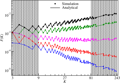
Figure 1: The probability for the occurrence of extreme events as a function of degree $k$, shown as log-log plot, for $\alpha=0.40,0.43,0.47,0.50,0.52$. Both the analytical (Eq. 4) and simulation results are shown. The shaded region on the left (right) corresponds to small degree nodes (hubs).

Physically, results in Fig 1 can be interpreted as follows. Note that $\alpha=1/2$ and $m=1$ in Eq. 5 represents the typical size $w_{typ}$ of flux through a node in the random walk environment. We can take the threshold $q_{i}$ to represent the capacity of the node to handle this flux $w_{typ}$. Then, $\alpha<1/2$ would imply $w_{typ}>q_{i}$, i.e, flux is more than the capacity of the node to handle it. This can be thought of as the congestion-like situation. On the other hand, $\alpha>1/2$ corresponds to $w_{typ}<q_{i}$, in which typical size of flux is smaller than the capacity of the node and hence congestion-like situation is less likely to happen. Fig. 1 implies that as $\alpha$ is varied, the probability of EE on the hubs shows larger variability than the small degree nodes (compare the shaded regions on the left and the right). Hence, we have far less control over the EE taking place on the small degree nodes. This is not the case for the hubs. The total number of EE on the entire network will depend on the events taking place on both the hubs and the small degree nodes. Thus, by adjusting the capacity or tuning $\alpha$, we can manipulate the EE taking place on scale-free network.

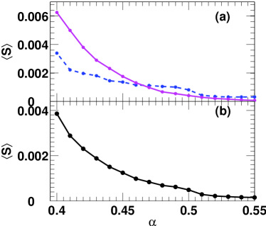
Figure 2: (a) The mean queue size $\langle S\rangle$ for the small degree nodes (dashed line) and the hubs (solid line), (b) the mean queue size for the entire network $\langle S\rangle$ plotted as a function of $\alpha$. Note that larger $\alpha$ correspond to larger nodal capacity.

II.2 Excess load as queue size

In any real network that encounters congestion-like situation, the traffic in excess of the nodal capacity leads to a build-up of queue. For instance, clustering of vehicles at the traffic junctions or pending http requests to a web server or phone connections waiting to be serviced by cellular hubs are all examples of such a build-up. If $\alpha<1/2$, we should expect to see such queue and the number of walkers waiting in that hypothetical queue or buffer [] is an indicator of the severity of the extreme event. In models in which queue does not get cleared, under certain conditions, jamming or a cessation of dynamics can take place. Phase transition to such a jamming state has been well studied jam . If $w_{i}(t)$ represents the number of walkers on $i$-th node at times $t=1,2,...T$, then the queue length is $Q_{i}(t)=(w_{i}(t)-q_{i})\theta\left(w_{i}(t)-q_{i}\right)$. In this, unit step function $\theta(.)$ is used to ensure that $Q_{i}(t)=0$ whenever $w_{i}(t)<q_{i}$. We define the mean queue size $\langle S\rangle$ for a network with $N$ nodes as

$$\langle S\rangle=\lim_{T\to\infty}\frac{1}{TN}\sum_{i=1}^{N}\sum_{t=1}^{T}Q_{i}(t)=\frac{1}{N}\sum_{i=1}^{N}f_{i}(w)Q_{i}$$ (6)

In this, $\langle S\rangle$ measures the mean number of walkers, in excess of nodal capacity, present in the queue per node at every time instant. Larger values of $\langle S\rangle$ imply more congestion-like scenario in the network. Now, we can obtain a broader picture of control over the extreme events as a function of $\alpha$. Fig. 2(b) shows the mean queue size $\langle S\rangle$ obtained from random walk simulations with $m=4$ as a function of $\alpha$. Evidently, $\langle S\rangle$ decreases with the increase in network capacity. Note that as argued before, $\alpha<0.5$ corresponds to a congestion-like situation and this is evident from the large values for $\langle S\rangle$. In contrast, for $\alpha>0.5$, $\langle S\rangle\approx 0$ indicating almost no extreme events on the network. Within the frame work of extreme events arising due to inherent fluctuations in the flux, it is impossible to eliminate them altogether and hence $\langle S\rangle$ will never be exactly zero. However, the probability of extreme event occurrence and the value of $\langle S\rangle$ can be made arbitrarily small by tuning $\alpha$.

Even as we manipulate the overall congestion-like scenarios on a network we explore the finer details. As Fig. 1 reveals, the extreme event probability on the hubs and small degree nodes have different dependence on degree $k$. This leads to an unequal apportioning of the burden of extreme events on hubs and small degree nodes of a network. We define a mean degree $\widetilde{k}$ such that we denote nodes with $k>\widetilde{k}$ as hubs and $k<\widetilde{k}$ as small degree nodes. Fig. 2(a) show $\langle S\rangle$ for hubs (solid line) and small degree nodes (dashed line) separately. For $\alpha<0.5$, hubs display larger queue sizes as compared with the small degree nodes. In a reversal of roles, for $\alpha>0.5$, hubs display small queue sizes when compared with the small degree nodes. Quite interestingly, at $\alpha\approx 0.47$, both the hubs and the small degree nodes equally share the burden of extreme events and queue sizes. This is indicated by the crossing of both the curves in Fig. 2(b). This is exactly the value of $\alpha$ at which the probability for extreme events becomes independent of degree $k$ in Fig. 1. Irrespective of how the hubs and small degree nodes are defined, $\alpha\approx 0.47$ would always remain the crossover point. Thus, except for $\alpha\approx 0.47$, the network does not share the burden of extreme events in an egalitarian manner among the small degree nodes and the hubs. The practical implication is that the designing nodal capacity implicitly affects the ’spatial’ distribution of extreme events over the nodes of a scale-free network.

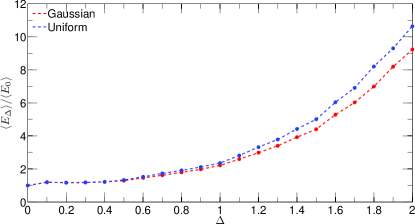
Figure 3: Scaled mean number of extreme events $\langle E_{\Delta}\rangle/\langle E_{0}\rangle$ with $m=4$ and $\alpha=1/2$ as a function of strength of noise $\Delta$. Random numbers were drawn from uniform and Gaussian distribution.

III Effect of variability in nodal capacity

In this section, we will take the capacity of $i$-th node to be $C_{i}=q_{i}$. The results in Sec. II implicitly assume that the capacity of $i$-th node $C_{i}$ is related to its degree $k_{i}$ through Eq. 5 and that all the nodes with identical degree have identical capacity. However, this condition is almost never satisfied in most of the real networks barrat ; motter1 . In reality, the nodal capacity of $i$-th node does not follow any prescribed formula and indeed could be treated as a random variable drawn from a suitable probability distribution. Hence, we have for the time-independent capacity of $i$-th node

$$C_{i}(\Delta)=\langle f_{i}\rangle+(m\sigma_{i}\pm\Delta\xi_{i}\sigma_{i})=C_{i}(0)\pm\Delta\xi_{i}\sigma_{i}$$ (7)

with $\Delta$ being the strength of noise and $\xi_{i}$ a random number. Evidently, if $\Delta=0$, this reduces to Eq. 5, the threshold for extreme events. We compute the mean number of extreme events over the entire network, i.e, $\langle E_{\Delta}\rangle=(1/NT)\sum_{t=1}^{T}\sum_{i=1}^{N}\theta(w_{i}(t)-C_{i}(\Delta))$, scaled by $\langle E_{0}\rangle$. Thus, after simple manipulations, we get,

$$\frac{\langle E_{\Delta}\rangle}{\langle E_{0}\rangle}=\frac{\sum_{i}F_{i}(C_{i}(\Delta))}{\sum_{i}F_{i}(C_{i}(0))}$$ (8)

By construction, this quantity is unity at $\Delta=0$. As simulations in Fig. 3 reveal, $\langle E_{\Delta}\rangle/\langle E_{0}\rangle$ for $m=4$ increases nonlinearly as the strength of noise $\Delta$ increases. It agrees with the analytical result obtained using Eqs. 8 and 4. Notice that Eq. 7 can be written as $C_{i}(\Delta)=\langle f_{i}\rangle+\widetilde{m}\sigma_{i}$ where $\widetilde{m}=m\pm\Delta\xi_{i}$, i.e, every node has a different value of capacity indexed by $\widetilde{m}$. We use the fact that the extreme event probabilities $F_{i}$ scale with magnitude netxv to obtain a leading order estimate of $\langle E_{\Delta}\rangle/\langle E_{0}\rangle\approx 1+a_{1}\Delta+a_{2}\Delta^{2}$, where $a_{1}$ and $a_{2}$ depends on the degree of the node. This conclusion is independent of whether the random numbers $\xi_{i}$ were drawn from uniform or Gaussian distribution.

Physically, this can be understood as follows. Suppose $C_{i}(0)$ represents $4\sigma$ capacity for all the nodes of the network. For noise strength $\Delta>0$, some nodes will have capacity $C_{-}$ such that $C_{-}<C_{i}(0)$ while others will have a capacity $C_{+}$ such that $C_{+}>C_{i}(0)$. The nodes with $C_{-}$ will encounter more extreme events and hence higher probability for the occurrence of extreme events (in comparison with $C_{i}(0)$ case). However for nodes with capacity $C_{+}$ the extreme event occurrence probability is much smaller and leads to fewer events. Hence we notice a net increase in the number of extreme events on $i$-th node. As $\Delta$ increases, this effect translates into an increase in the mean number of extreme events over the entire network. In most of the real-life networks, the nodal capacity is typically proportional to the flux passing through the node betcen but is unlikely to adhere strictly to specifications such as $C(0)$ assumed in Eq. 7. Hence it is an appropriate guess that nodal capacity being proportional to its importance as measured by degree could be its mean behaviour barrat but the actual capacities would be a random variable cap clustered around this mean behaviour. In all such cases, the random walk based model studied here predicts that the number of extreme events will increase with the variability in the nodal capacity. For other values of $\alpha$ too qualitatively similar results as in Fig. 3 are obtained.

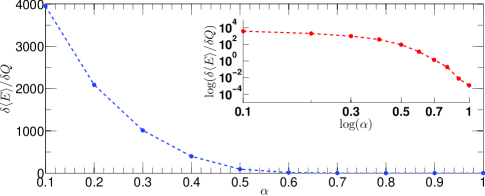
Figure 4: The ratio of change in mean number of extreme events $\delta\langle E\rangle$ on the network for $\delta C$ change in capacity of the network plotted as a function of $\alpha$. This is obtained from random walk simulations (solid circles) with $m=4$. The inset shows the same data in log-log plot.

IV Capacity addition and extreme events

Given that the variability in the nodal capacity leads to an overall increase in the number of extreme events (as shown in Fig. 3), we ask how we can reduce the mean number of extreme events on the network. This would be a desirable requirement for a smooth functioning of the networks cec . As argued before, intuitively we expect mean number of extreme events to decrease if nodal capacity increases. We can increase capacity by increasing $\alpha$. Further, to simplify the scenario, we take $\Delta=0$ for this part. Figure 4 shows simulation results for the change in the mean number of extreme events when capacity changes by one unit, i.e, $\delta\langle E\rangle/\delta C$ as a function of $\alpha$. For $\alpha<0.5$, the $\delta\langle E\rangle/\delta C$ curve decays quickly. In this regime, capacity addition is accompanied by a large reduction in the number of extreme events. Hence, any capacity addition in this regime yields rich dividends in terms of cost-benefit ratio. However, beyond $\alpha\approx 0.5$, $\delta\langle E\rangle/\delta C$ is vanishingly small indicating no significant change in the number of extreme events even when the capacities are increased. When $\alpha>0.7$, $\delta\langle E\rangle<1$, i.e, less than 1 extreme event on an average. In this regime, capacity increase is not beneficial in alleviating the extreme events. Since capacity addition (like building bridges, for instance) is generally an expensive proposition, we emphasize the following important implication of this result. If the aim is to control the mean number of extreme events on a scale-free network even while maintaining a certain reasonable level of cost-benefit ratio, it is important to apriori estimate if we operate in the regime in which cost-benefit ratio is favourable. The results obtained in this work provides insights into nodal capacity addition vis-a-vis reduction in EE. We emphasise that qualitatively similar results are obtained even when $\Delta>0$.

V conclusions

In this work, we have studied the extreme events induced by inherent fluctuations in the flux and taking place on scale-free networks. Given that such inherent fluctuations are unavoidable in any finite network, we show that it is possible to tune, either increase or decrease, the probabilities for the occurrence of extremes in flux on a scale-free network using nodal capacity as a tunable parameter. This requires that the degree distribution have a large support of at least two orders of magnitude (see $x$-axis in Fig. 1). This is not true of Erdos-Renyi networks with sharply peaked degree distributions and hence these results will not hold good for them. As we tune the nodal capacity, we show how various parts of the network share the burden of extreme events and we discuss its implications. Further we study the effect of variability in the nodal capacity. We show that larger variability in the nodal capacity of scale-free networks leads to more extreme events.

On the other hand, as we intuitively expect, increasing nodal capacity and hence the capacity of the entire network leads to decrease in the mean number of extreme events in the network. One significant result of this work is displayed in Fig. 4. This shows that increasing capacity beyond certain level does not lead to proportionate decrease in the incidences of extreme events. This has important implications for network design efforts. Since increasing the capacity of network is an expensive proposition in almost all the real-life situations, this work provides an important theoretical benchmark to understand the limitations of capacity addition as a route to alleviate extreme events. In general, real life situations involving transport on scale-free networks are generally more complex than the random walk scenarios studied here vesp . However, this work sets the benchmark against which to understand extreme events arising from other types of transport processes on networks. Further, based on evidence from earlier studies netxv , it is possible that even if random walk is replaced by a more intelligent routing algorithm, the results of this work might qualitatively remain valid.

All the simulations were done on the computer cluster at IISER Pune. ARS thanks DST for the financial support during the time this work was done.

References

- (1) A. Vespignani, Nature Physics 8, 32 (2012).
- (2) Vimal Kishore, M. S. Santhanam and R. E. Amritkar, Phys. Rev. Lett. 106, 188701 (2011).
- (3) Vimal Kishore, M. S. Santhanam and R. E. Amritkar, Phys. Rev. E. 85, 056120 (2012).
- (4) A. S. Sharma, A. Bunde, V. P. Dimri, and D. N. Baker (ed.), Extreme events and natural hazards : The complexity perspective, Geophysical Monograph Series 196, (AGU, Washington, D. C); S. Albeverio, V. Jentsch and Holger Kantz (Ed.) , Extreme events in nature and society, (Springer, 2005).
- (5) Texas Transportation Institute’s 2012 Urban Mobility Report, D. Schrank, B. Eisele and T. Lomax, (2012). (Available at mobility.tamu.edu); K. Fisher-Vanden, E. T. Mansur and Q. Qang, National Bureau of Economic Research Working Papers, Working paper 17741. (Available at www.nber.org/papers/w17741).
- (6) Y. Liu, J. Slotine and A. L. Barabasi, Nature 473, 167 (2011); ibid, PLOS ONE 7, e44459 (2012); V. Nicosia et. al., Scientific Reports 2, 218 (2012); T. Nepusz and T. Vicsek, Nature Physics 8, 568 (2012); M. Posfai et. al., Scientific Reports 3, 1067 (2013).
- (7) J. D. Noh and H. Reiger, Phys. Rev. Lett. 92, 118701 (2004); M. Rosvall and C. T. Bergstrom, PNAS 105, 1118 (2008). N. Zlatanov and L. Kocarev, Phys. Rev. E 80, 041102 (2009).
- (8) L. F. Costa and G. Travieso, Phys. Rev. E. 75, 016102 (2007); V. Tejedor et. al., Phys. Rev. E. 80, 065104(R) (2009).
- (9) J. F. Eichner et. al., Phys. Rev. E 75, 011128 (2007); M. S. Santhanam and Holger Kantz, Phys. Rev. E 78, 051113 (2008).
- (10) S. Meloni et. al., Phys. Rev. Lett. 100, 208701 (2008).
- (11) A. Barrat et. al., PNAS 101, 3747 (2004).
- (12) Dong-Hee Kim and A. Motter, New J. Phys 10, 053022 (2008).
- (13) M. Abramowitz and I. A. Stegun, Handbook of Mathematical Functions (Dover, New York, 1964).
- (14) A. Arenas, A. Diaz-Guilera and R. Guimera, Phys. Rev. Lett. 86, 3196 (2001); D. De Martino, L. Dall’Asta, G. Bianconi and M. Marsili, Phys. Rev. E 79, 015101(R) (2009); B. Tadic, G. J. Rodgers and S. Thurner, Int. J. Bif. and Chaos 17, 2363 (2007); A. S. Stepanenko et. al., EPL 100, 36002 (2012).
- (15) Most of the work that uses shortest-path routing algorithms assume typical size of flux through the nodes to be proportional to betweenness centrality. P. Holme and B. J. Kim, Phys. Rev. E 65, 066109 (2002); G. Yan et. al., Phys. Rev. E 73, 046108 (2006).
- (16) W. L. Tan, F. Lam and W. C. Lau, IEEE Trans. Mob. Comput. 7, 737 (2008).
- (17) G. Zhang, EPL 89, 38003 (2010).