Transport and STM studies of hyperbolic surface states of topological insulators

Abstract

Motivated by the transmission of topological surface states through atomic scale steps, we study the transport of gapless Dirac fermions on hyperbolic surfaces. We confirm that, independent of the curvature of the hyperbolae and the sharpness of the corners, no backward scattering takes place and transmission of the topological surface states is completely independent of the geometrical shape (within the hyperbolic model) of the surface. The density of states of the electrons, however, shows a dip at concave step edges which can be measured by an STM tip. We also show that the tunneling conductance measured by a polarized scanning tunneling probe exhibits an unconventional dependence on the polar and azimuthal angles of the magnetization of the tip as a function of the curvature of the surface and the sharpness of the edge.

I Introduction

Interest in topological insulators (TIs) continues to remain high ever since their predictiontheory and discoverykonig . The hallmark of these materials is their topologically non-trivial nature, due to which they have gapless linearly dispersing edge states, although they are insulating in the bulkreviews . Such edge states are familiar in the two-dimensional quantum Hall systemqhereviews , but in TIs, they arise even in higher dimensional systems and even in the absence of time-reversal symmetry breaking.

For two-dimensional TIs, the edge states consist of two counter-propagating modes, with opposite spin projections. The correlation of the spin of the electron with its direction of motion is the central feature of these states. The existence of these states have been verified experimentally by measurements in the HgTe quantum well structureskonig . There have also been several theoretical studies vari ; das ; soori , studying consequences of the spin projection and the helical nature of the edge states, although there has been no direct measurement of the spin of the edge states.

The three dimensional TIs come in two classes, strong and weak, with even and odd number of Dirac cones on its surface. For strong TIs, the existence of an odd number of Dirac cones is topologically protected and it has been found that the surface states of strong TIs such as $HgTe,Bi_{2}Se_{3}$ and $Bi_{2}Te_{3}$ can be described by a single Dirac electron. These surface states are robust against perturbations that do not break time-reversal symmetry. The electrons also have the feature that their spin is ‘locked’ to the momentum of the electron, which is what leads to a complete absence of back-scattering, because the spin of the electrons at momentum ${\bf k}$ is orthogonal to the spin of the electrons at momentum $-{\bf k}$. The combination of topological stability and absence of backward scattering leads to the prediction that the surface states of TIs wrap the surface of the TI and are impervious to the existence of surface defects. This has been confirmed by experiments which not only have confirmed the absence of backward scatteringtzhang ; roushan , but more recently have also shown full transmission through atomic step edgesseo . This would imply that transport through these surface states is independent of the geometrical shape of the surface.

With a few notable exceptionsimura1 ; imura2 ; imura3 , most of the theoretical work on TIs has been restricted to planar surfaces and straight line edges. For instance, the original derivation of the edge states was for samples with a single straight edge. This was extended to the case for finite strips where it was shown that there was some interference between the two edgeszhou . However, there had been no direct study of what happens when two sharp edges meet one another. Since spin projection is tied to the direction of motion, it is also not clear how the spin current changes if there are sharp edges. Similarly, although there have been some studiesjiang ; takahashi ; diptiman ; krishnendu of what happens at junctions of two 3DTIs, the extension of the gapless Dirac state over curved surfaces has yet to be demonstrated.

A step in this direction was recently taken by Takane and Imuratakane , who introduced a hyperbolic system to treat the $90^{\rm o}$ step edge, and by introducing appropriate curvilinear coordinates, they could show that no reflection takes place at the $90^{\rm o}$ step edge, and transmission was perfect, although there was a sharp change in the expectation value of spin in the close vicinity of the step. In this paper, we generalise their work to step edges of arbitrary angles, and show that independent of the curvature of the hyperbolae and the sharpness of the corners, no backward scattering takes place and the transmission of the topological surface states is completely independent of the geometrical shape (within the hyperbolic model) of the surface. Moreover, we study how the density of states (DOS) and the spin DOS behave as a function of the curvature and the sharpness of the edge of any sample. We find that the DOS shows a dip at the concave edges of the sample. We also compute the tunneling conductance measured by a polarized scanning tunneling microscope, as a function of the curvature of the surface and the sharpness of the edges and show that the STM conductance has a non-trivial dependence on the curvature angle $\phi$ and an unconventional dependence on the polar and azimuthal angles of the tip, which are not displayed by a planar TI surface.

II The model and analysis

We start with the continuum model of a strong anisotropic TI in 3D, given by the Hamiltonianhzhang

$$H_{\rm bulk}=\begin{pmatrix}{}m({\bf p})\tau_{z}+A_{z}p_{z}\tau_{x}&(A_{x}p_{x}-iA_{y}p_{y})\tau_{x}\\ (A_{x}p_{x}+iA_{y}p_{y})\tau_{x}&m({\bf p})\tau_{z}-A_{z}p_{z}\tau_{x}\end{pmatrix}~{}.$$ (1)

The parameters $A_{x},A_{y},A_{z}$ and $m({\bf p})$ can be determined for specific materials by comparing with the ab initio calculations of the effective model of 3DTIhzhang . Here, the $2\times 2$ matrix represents the spin degrees of freedom and the orbital degrees of freedom are represented by the Pauli matrices $\tau_{i}$. The mass term $m({\bf p})=m_{0}+m_{2}(p_{x}^{2}+p_{y}^{2}+p_{z}^{2})$ in this 3D Dirac Hamiltonian is momentum dependent. For the topological insulator, we need to take $m_{0}>0$ and $m_{2}<0$. Assuming the system to be translationally invariant in the $x$ direction, so that $p_{x}$ is a good quantum number, it is straightforward to derive the surface states on either the $xy$ plane or the $xz$ plane. However, it is not obvious what happens close to the corners. Takane and Imuratakane studied the question of whether or not there exists reflection at the corners for non-zero $p_{x}$ by assuming that the surface could be represented by a rectangular hyperbolic model using curvilinear coordinates. In this paper, we assume that the surface of the TI can be an arbitrary hyperbolic surface as shown in Fig. (1a). Note that we are representing a concave surface - the TI is in the shaded region as shown in the figure. The curve in Fig. (1b) can be described by the equation

$$(az)^{2}-y^{2}=R^{2}$$ (2)

where the angle between the two asymptotic surfaces is governed by the (curvature) parameter $a$ and the sharpness at the edge is governed by the (sharpness) parameter $R$. The 3D TI is translationally invariant in the $x$-direction. A separable coordinate system can now be defined as follows -

$$y = -r\cos\phi+y_{0}(\phi),$$

$$z = -r\sin\phi+z_{0}(\phi),$$ (3)

where $y_{0}$ and $z_{0}$ define the curve and are given by

$$y_{0} = \frac{-aR\cot\phi}{\sqrt{1-a^{2}\cot^{2}\phi}}$$

$${\rm and}~{}~{}z_{0} = \frac{R}{a}\frac{1}{\sqrt{1-a^{2}\cot^{2}\phi}}~{}.$$ (4)

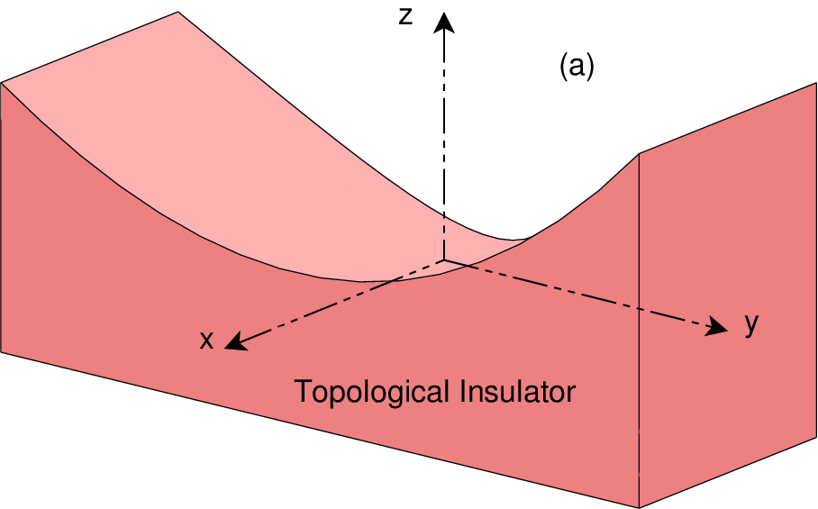
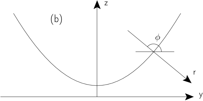
Figure 1: The surface is shown (above) in Fig.(1a) with the TI filling the concave part and the curvilinear coordinate system is shown (below) in Fig.(1b) as described in the text.

We draw normals to the surface as shown in Fig. (1b) and define $\phi$ as the angle between the normal and the $y$-axis, and define $r$ as the distance (in the direction shown by the arrow) from the surface. It is easy to see that $\phi$ ranges from $\tan^{-1}(a)$ to $\pi-\tan^{-1}(a)$ and $r$ ranges from $-\infty$ to $\infty$. The Jacobian of the transformation can be easily found to be given by $r+f(\phi)$, where

$$f(\phi)=\frac{Ra\operatorname{cosec}^{3}\phi}{(1-a^{2}\cot^{2}\phi)^{3/2}}~{}.$$ (5)

We can now define the mass term $m({\bf p})$ in terms of $p_{r}$,$p_{\phi}$ and $p_{x}$ - $i.e.$, $m({\bf p})=m_{r}+m_{\phi}+m_{x}$ with

$$m_{r} = m_{0}-m_{2}[\partial_{r}^{2}+(r+f)^{-1}\partial_{r}],$$

$$m_{\phi} = -m_{2}[(r+f)^{-2}(\partial_{\phi}^{2}-(r+f)^{-}(\partial_{\phi}f)\partial_{\phi}),$$

$${\rm and}~{}~{}m_{x} = m_{2}p_{x}^{2}~{}.$$ (6)

The bulk Hamiltonian $H=m({\bf{p}})\tau_{z}+(A_{x}p_{x}\sigma_{x}+A_{y}p_{y}\sigma_{y}+A_{z}p_{z}\sigma_{z})\tau_{x}$ can now be written in terms of the curvilinear coordinates $(r,\phi,x)$ as

$$H_{\rm bulk}=H_{r}+H_{\phi}+H_{x}$$

with

$$H_{r} = \left(\begin{array}[]{cc}m_{r}\tau_{z}+iA_{z}\sin(\phi)\partial_{r}\tau_{x}&A_{y}\cos(\phi)\partial_{r}\tau_{x}\\ -A_{y}\cos(\phi)\partial_{r}\tau_{x}&m_{r}\tau_{z}-iA_{z}\sin(\phi)\partial_{r}\tau_{x}\end{array}\right),$$ (9)

$$H_{\phi} = \left(\begin{array}[]{cc}m_{\phi}\tau_{z}+iB_{z}\tau_{x}&-B_{y}\tau_{x}\\ B_{y}\tau_{x}&m_{\phi}\tau_{z}-iB_{z}\tau_{x}\end{array}\right),~{}~{}{\rm and}$$ (12)

$$H_{x} = \left(\begin{array}[]{cc}m_{x}\tau_{z}&A_{x}p_{x}\tau_{x}\\ A_{x}p_{x}\tau_{x}&m_{x}\tau_{z}\end{array}\right)~{}.$$ (15)

We have used $B_{z}=A_{z}(r+f)^{-1}\cos(\phi)\partial_{\phi}$ and $B_{y}=A_{y}(r+f)^{-1}\sin(\phi)\partial_{\phi}$ in $H_{\phi}$ above. Note that for a rectangular hyperbolic surface with $a=1$, our surface and expressions are equivalent to to those given in Ref.takane , albeit rotated by $\pi/4$ about the $x$-axis.

To derive the effective 2D surface $(\phi,x)$ Hamiltonian from the above bulk Hamiltonian, we need to first solve the radial equation $H_{r}|\psi\rangle=E_{r}|\psi\rangle$. Following Refs.takane ; imura1 , we obtain a solution of the form $|\psi\rangle=e^{-\kappa r}|u\rangle$, where $\kappa^{-1}$ measures penetration into the bulk, provided that we assume that $(r+f)^{-1}=\langle(r+f)^{-1}\rangle\equiv\Gamma^{-1}$ in $H_{r}$ where the average value $\Gamma^{-1}$ is defined later. As shown in Ref.imura1 , the boundary condition of $\psi({\bf r}=0)=0$ holds when we choose $E_{r}=0$. This gives us the values of $\kappa$ as

$$\kappa_{\pm} = \frac{\tilde{A}_{\phi}\pm\sqrt{\tilde{A}^{2}_{\phi}+4m_{0}m_{2}}}{-2m_{2}}$$ (16)

$$= \frac{\tilde{A}_{\phi}}{-2m_{2}}\left[1\pm\sqrt{1+\frac{4m_{0}m_{2}}{\tilde{A}^{2}_{\phi}}}\right]$$

where $\tilde{A}_{\phi}\equiv A_{\phi}-\Gamma^{-1}m_{2}$ and $A_{\phi}=\sqrt{A_{y}^{2}\cos^{2}(\phi)+A_{z}^{2}\sin^{2}(\phi)}$. We can also get solutions with $\tilde{\kappa}$ being the negative of the expressions on the RHS. But since it is only the positive values which are compatible with the boundary condition that the states are localized near the surface, we focus our attention only on the positive solutions $\kappa_{\pm}$. To find the eigenvectors, we note that

$$\left(\begin{array}[]{cc}\tau_{z}&0\\ 0&\tau_{z}\end{array}\right)H_{r}(K)=$$ (19)

$$\left(\begin{array}[]{cc}m_{r}(K)+A_{z}\sin(\phi)K\tau_{y}&-iA_{y}\cos(\phi)K\tau_{y}\\ iA_{y}\cos(\phi)K\tau_{y}&m_{r}(K)-A_{z}\sin(\phi)K\tau_{y}\end{array}\right)$$ (22)

$$=m_{r}(K)\mathbb{I}+K(A_{z}\sin(\phi)\sigma_{z}+A_{y}\cos(\phi)\sigma_{y})\tau_{y}$$

$$=m_{r}(K)\mathbb{I}+A_{\phi}K\left(\sin(\tilde{\phi})\sigma_{z}+\cos(\tilde{\phi})\sigma_{y}\right)\tau_{y}~{},$$ (23)

where in the last line we have used $e^{i\tilde{\phi}}={(A_{y}\cos{\phi}+iA_{z}\sin{\phi})}/{A_{\phi}}$. We then obtain the two basis (normalised) eigenstates of $H_{r}$ given by $|\psi_{\pm}\rangle=\mathcal{N_{\phi}}\rho(r,\phi)|u\pm\rangle$ where $\rho(r,\phi)=e^{-K_{+}r}-e^{-K_{-}r}$,

$$|u\pm>=\frac{1}{\sqrt{2}}\left(\begin{array}[]{c}\sin\left(\frac{\tilde{\phi}}{2}\mp\frac{\pi}{4}\right)\left(\begin{array}[]{c}1\\ \pm i\end{array}\right)\\ i\cos\left(\frac{\tilde{\phi}}{2}\mp\frac{\pi}{4}\right)\left(\begin{array}[]{c}1\\ \pm i\end{array}\right)\end{array}\right)~{},$$ (24)

and $\mathcal{N_{\phi}}$ is a $\phi$ dependent normalisation factor. The convention chosen above is such that $|\psi_{+}\rangle$ corresponds to the solution in which spin is pointing along the negative $r$ direction (ie outside the insulator) and the spin for $|\psi_{-}\rangle$ points along the positive $r$ direction (inside the insulator). Note that the direction of the real spin is determined by the angle $\tilde{\phi}$, which depends on the values of $a$, which determines the curve of the surface and also $A_{y}$ and $A_{z}$ which are material dependent parameters. It also varies as a function of $\phi$ , as we sweep the surface across the range of $\phi$. But it is always parallel to the surface, as is expected from spin-momentum locking.

Now, let us derive the effective 2D surface Hamiltonian in the $|\psi\pm\rangle$ space. Any surface state $|\chi\rangle$ can be represented as $|\chi\rangle=\chi_{+}|\psi_{+}\rangle+\chi_{-}|\psi_{-}\rangle$. We can now define a two component spinor $\chi=(\chi_{+},\chi_{-})^{T}$ and define the effective Hamiltonian for $\chi$ as

$$H_{\rm eff}=\begin{pmatrix}\langle\psi_{+}|H_{\phi}+H_{x}|\psi_{+}\rangle&\langle\psi_{+}|H_{\phi}+H_{x}|\psi_{-}\rangle\\ \langle\psi_{-}|H_{\phi}+H_{x}|\psi_{+}\rangle&\langle\psi_{-}|H_{\phi}+H_{x}|\psi_{-}\rangle\end{pmatrix}.$$ (25)

Note that $+$ and $-$ refers here to real spin-up and spin-down, but the quantisation axis, and hence the meaning of spin up and down, continuously changes along the hyperbolic surface. We shall essentially follow the same steps as in Ref.takane to compute the effective Hamiltonian. To simplify the notation, we define $\theta_{\pm}={\tilde{\phi}}/{2}\mp{\pi}/{4}$. We find that the diagonal elements $\langle\psi_{\pm}|H_{\phi}+H_{x}|\psi_{\pm}\rangle=0$ and the off-diagonal elements are given by

$$\langle\psi_{\pm}|H_{\phi}+H_{x}|\psi_{\mp}\rangle=\tilde{\mathfrak{H}}_{\pm},$$ (26)

where

$$\tilde{\mathfrak{H}}_{\pm}=\mp\frac{\tilde{\mathcal{A}}_{\phi}}{\langle r\rangle+f}\partial_{\phi}\mp\frac{1}{2}\partial_{\phi}\left(\frac{\tilde{\mathcal{A}}_{\phi}}{\langle r\rangle+f}\right)-A_{x}p_{x}$$

and $$\tilde{\mathcal{A}}_{\phi}=\left[A_{\phi}-m_{2}\Gamma^{-1}\right]\left(\partial_{\phi}\tilde{\phi}\right)~{}.$$

In the above equations, we have used

$$\int_{0}^{\infty}dr\left[\mathcal{N}_{\phi}\rho(r,\phi)\right]^{2} = \frac{\int_{0}^{\infty}dr\rho^{2}(r,\phi)}{\int_{0}^{\infty}dr(r+f)\rho^{2}(r,\phi)}$$ (27)

$$= \frac{1}{\langle r\rangle+f}$$

where

$$\langle r\rangle=\frac{\int_{0}^{\infty}drr\rho^{2}(r,\phi)}{\int_{0}^{\infty}dr\rho^{2}(r,\phi)}~{}.$$ (28)

We have also used

$$\Gamma^{-1}=\frac{\int dr(r+f)^{-1}\rho^{2}}{\int dr\rho^{2}}$$ (29)

and

$$\int_{0}^{\infty}dr\mathcal{N}_{\phi}\rho(r,\phi)\partial_{\phi}\left(\mathcal{N}_{\phi}\rho(r,\phi)\right)$$

$$=\frac{1}{2}\partial_{\phi}\left(\int_{0}^{\infty}dr\left[\mathcal{N}_{\phi}\rho(r,\phi)\right]^{2}\right)=\frac{1}{2}\partial_{\phi}\left(\frac{1}{\langle r\rangle+f}\right).$$ (30)

As was done in Ref.takane , it is convenient to define a length variable, instead of the angle variable $\phi$ as

$$l=\int_{\frac{\pi}{2}}^{\phi}d\phi^{\prime}\langle r\rangle(\phi^{\prime})+f(\phi^{\prime})$$ (31)

located just below the geometric surface. The limits of $\phi\rightarrow\tan^{-1}a,\pi-\tan^{-1}a$ correspond to $l\rightarrow-\infty,+\infty$. Since the probability density must not change during this transformation, ${\tilde{\chi}}_{\pm}(l)$ is related to $\chi_{\pm}(\phi)$ as

$${\tilde{\chi}}(l)=\frac{{\chi}(\phi(l))}{\sqrt{\langle r\rangle+f}}~{}.$$ (32)

Hence, we can solve the eigenvalue equation $H_{\rm eff}\chi_{\pm}=E\chi_{\pm}$ on the entire hyperbolic surface, by transforming $\tilde{\mathfrak{H}}_{\pm}{\chi}(\phi)=E{\chi}(\phi)$ to

$$\mathfrak{H}_{\pm}{\tilde{\chi}}(l)=E{\tilde{\chi}}(l)~{},$$ (33)

where $\mathfrak{H}_{\pm}$ is now given by

$$\mathfrak{H}_{\pm}=\mp\tilde{\mathcal{A}}_{l}\partial_{l}\mp\frac{1}{2}\partial_{l}\left(\tilde{\mathcal{A}}_{l}\right)-A_{x}p_{x}~{},$$ (34)

and $\tilde{\mathcal{A}}_{l}$ can be considered the effective velocity of the electron along the coordinate $l$ which is effectively increased due to the effect of the Jacobian dependent second term in $\tilde{\mathcal{A}}_{\phi}$. We focus on eigenstates with energy $E=\sqrt{(Ak)^{2}+(A_{x}k_{x})^{2}}$ and obtain the two surface solutions as

$${{\tilde{\chi}}}_{\pm}=\sqrt{\frac{1}{2\tilde{\mathcal{A}}_{l}}}\left(\begin{array}[]{c}1\\ -e^{\mp i\zeta}\end{array}\right)e^{\pm i\int^{l}dl^{\prime}\frac{Ak}{\tilde{\mathcal{A}}_{l^{\prime}}}+ik_{x}x}$$ (35)

The factor of $\sqrt{2}$ above ensures that the probablity density current in the direction of $l$ is $\pm\frac{Ak}{E}$ as it should be for a free Dirac particle of momentum $k$ and energy $E$. Hence, as expected, we get surface states satisfying the Dirac equation. However, unlike on a planar surface, the definition of $Ak$ changes as we change $l$. Since these wave-functions are valid everywhere on the hyperbolic surface, it is clear that no backward scattering takes place anywhere and that the transmission is unity along any path independent of the shape and size of the curvature of the surface. Thus, we generalise the earlier result takane which concluded that there was no reflection at a $90^{o}$ corner and find that there is no reflection even when the corner has any angle other than $90^{o}$.

III Density of states and tunneling current for polarised STM

III.1 Density of states

Although there is no reflection on the curved surface, the density of states does change as a function of both the curvature and the sharpness of the corners. The local density of states (DOS) is defined as

$$\rho_{s}=\int d\omega[f(\omega)-f(\omega+eV)]\sum_{\nu}\delta(E_{\nu}-eV)|{\tilde{\chi}}_{\pm}|^{2}$$ (36)

and is clearly a function of the curvature parameter $a$ and the sharpness parameter $R$ through the wave-function ${\tilde{\chi}}_{\pm}$. We will restrict ourselves to low biases and low temperatures and normalize the DOS by its value at $\phi=\tan^{-1}a$. In Figs. (2a) and (2b), we show the DOS as a function of the angle parameter $\phi$ which spans the surface. Note that the DOS shows a dip at $\phi=\pi/2$ (or $l=0$), which is the point of maximum curvature, both for fixed $R$ in Fig. (2a) as well as for fixed $a$ in Fig. (2b). Note also that in Fig. (2a), the range of $\phi$ depends on the curvature parameter $a$ and increases as the curvature increases, whereas in Fig. (2b), the range is fixed from $\tan^{-1}a=\pi/4$ to $\pi-\tan^{-1}a=3\pi/4$ for $a=1$. From both the curves, it is clear that in the limit of a planar surface ($a\rightarrow\infty$ or $R\rightarrow\infty$), the DOS is flat, as is expected for the usual planar TIs.

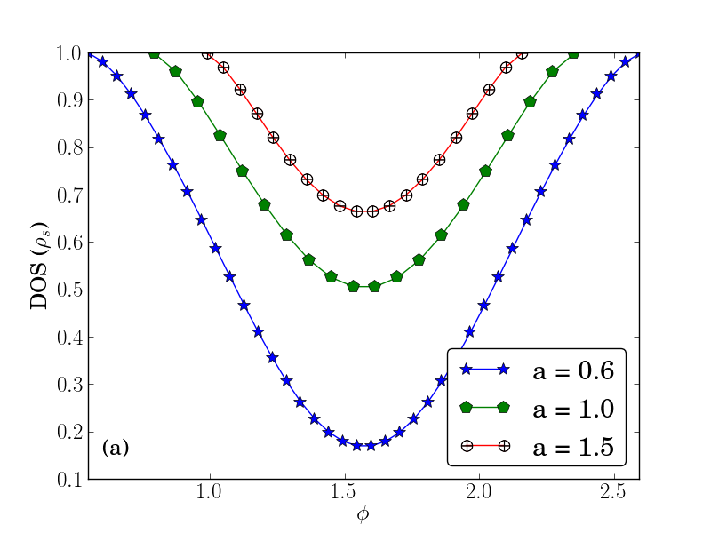
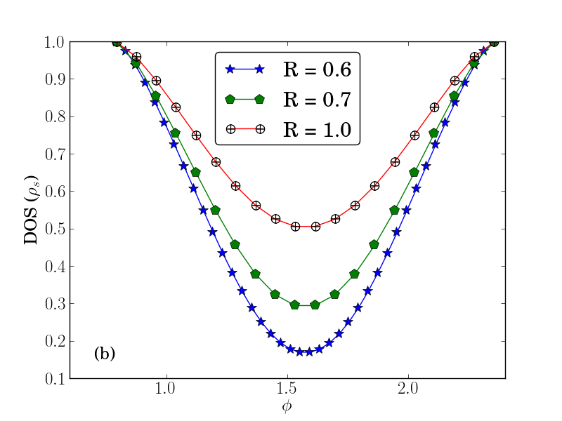
Figure 2: The DOS as a function of the angle parameter $\phi$ along the surface, for fixed sharpness $R=1$ and for three different curvatures, normalised to unity at $\phi=\tan^{-1}a$, is shown in Fig. (2a), while in Fig. (2b), it is shown for three different values of the sharpness parameter and for fixed curvature $a=1$.

III.2 Tunneling current for a polarized STM tip

We now use the theory for the tunneling current of Dirac electrons on the surface of a TI, developed in Ref.krishnendu . By using the Bardeen tunneling formulabardeen , and explicitly computing the matrix element for overlap between the tip and the material wave-functions, they found that the tunneling current at zero temperature was given by

$$I(V) = I_{0}|c_{0}|^{2}\rho_{t}[\rho_{d}+\rho_{z}\cos\alpha+\rho_{m}\sin\alpha]$$

$$\times \int d\omega[f(\omega)-f(\omega+eV)]$$

$${\rm with}~{}~{}\rho_{d} = \sum_{\nu}\delta(E_{\nu}-eV)|\psi_{\uparrow\nu}|^{2}(1+\kappa_{\nu}^{2})$$

$$\rho_{z} = \sum_{\nu}\delta(E_{\nu}-eV)|\psi_{\uparrow\nu}|^{2}(1-\kappa_{\nu}^{2})$$

$$\rho_{m} = \sum_{\nu}\delta(E_{\nu}-eV)|\psi_{\uparrow\nu}|^{2}\kappa_{\nu}\cos(\beta-\eta_{\nu})~{}.$$ (37)

Here $c_{0}$ is a constant which depends on details of the tip wave-function and $\rho_{t}$ is the density of states for the tip electron, assumed to be constant. However this was derived using a flat surface for the topological insulator with the spin quantisation axis of the electrons fixed to be in the ${\hat{z}}$-direction. In this basis, the tip wave-function was represented as

$$\psi_{t}=\begin{pmatrix}{}\cos(\alpha/2)\\ ~{}~{}~{}~{}\sin(\alpha/2)e^{i\beta}\end{pmatrix}$$ (38)

and the electron wave-function on the surface was given by

$$\psi_{\nu}({\bf r};z)=\begin{pmatrix}\psi_{\uparrow\nu}({\bf r};z)\\ \psi_{\downarrow\nu}({\bf r};z)\end{pmatrix}=\begin{pmatrix}1\\ \kappa_{\nu}e^{-i\eta_{\nu}}\end{pmatrix}\psi_{\uparrow\nu}~{}.$$ (39)

But for the hyperbolic surface, the spin quantisation axis is continuously changing as a function of the curvature - i.e., as a function of the angle $\phi$, due to spin-momentum locking. Hence, to express the tip wave-function in the basis of the electron spin quantisation axis, we need to rotate the spinor by $\phi-\pi/2$ and obtain it in the $\phi$-basis, the basis which is perpendicular to the surface. In this basis, the tip wave-function is given by

$$\psi_{t}^{\phi}=\begin{pmatrix}{}C\cos(\alpha/2)-iS\sin(\alpha/2)e^{i\beta}\\ -iS\cos(\alpha/2)+C\sin(\alpha/2)e^{i\beta}\end{pmatrix}$$ (40)

where $C=\cos(\phi/2-\pi/4)$ and $S=\sin(\phi/2-\pi/4)$. Note that we have rotated the basis in the counter-clockwise direction about the $x$-axis, and have chosen the $\phi$-axis to be pointing out of the TI - $i.e.$, opposite the normal direction defined by $r$.

Now to be able to use the expression for the current given in Eq.37, we need to rewrite the spinor given in Eq.40 in the form given in Eq.38. We find that $\psi_{t}^{\phi}$ can be written as

$$\psi_{t}^{\phi}=e^{i\xi}\begin{pmatrix}{}\cos({\tilde{\alpha}/}2)\\ ~{}~{}~{}~{}\sin({\tilde{\alpha}}/2)e^{i{\tilde{\beta}}}\end{pmatrix}$$ (41)

where

$$\cos{\tilde{\alpha}} = -\cos{\phi}\sin{\alpha}\sin{\beta}+\sin\phi\cos{\alpha},$$

$$\tan{\tilde{\beta}} = \tan\beta\sin\phi+\cos\phi\sec\beta\cot\alpha$$ (42)

and the overall (unimportant) phase of the spinor is given by

$$\tan\xi=-\frac{\tan(\frac{\alpha}{2})\cos(\beta)\tan(\frac{\phi}{2}-\frac{\pi}{4})}{1+\tan(\frac{\alpha}{2})\sin(\beta)\tan(\frac{\phi}{2}-\frac{\pi}{4})}~{}.$$ (43)

The wave-function of the electron on the curved surface has been derived in Eq.35. Comparing with the wave-function in Eq.39, we see that $\kappa_{\nu}=-1$ and $\eta_{\nu}=\pm\zeta$. Now, we can use the expressions given in Eq.37 to compute the tunneling conductance as

$$G = G_{0}|c_{0}|^{2}\rho_{t}[\rho_{d}+\rho_{z}\cos{\tilde{\alpha}}+\rho_{m}\sin{\tilde{\alpha}}]$$

$${\rm with}~{}~{}\rho_{d} = {\frac{1}{2{\tilde{A}}}}\sum_{\nu}\delta(E_{\nu}-eV),$$

$$\rho_{z} = 0$$

$${\rm and}~{}~{}\rho_{m} = -{\frac{1}{2{\tilde{A}}}}\sum_{\nu}\delta(E_{\nu}-eV)\cos({\tilde{\beta}}\mp\zeta)~{}.$$ (44)

where $G_{0}=2e^{2}/h$. $\rho_{z}=0$ because $\kappa_{\nu}=-1$ , which is a result of spin-momentum locking, due to which the spin of the electron lies along the surface perpendicular to the quantization axis. However, $\rho_{d}$ and $\rho_{m}$ are non-zero and both show non-trivial dependence on $\phi$ (or $l$). In Fig.(3), the tunneling conductance has been plotted as a function of $l$ for various values of the curvature $a$ with fixed sharpness parameter $R$ (for fixed tip parameters $\alpha$ and $\beta$). Note that unlike the case for a flat surface for which the STM conductance is constant, (reproduced here in the large $a$ limit), here the STM conductance varies as it spans the curved surface and shows a dip precisely at $l=0$. This dip depends on the curvature and increases as the curvature increases.

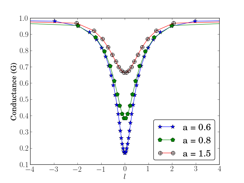
Figure 3: Tunneling conductance $G$ (normalised to unity at $l\rightarrow-\infty$) for fixed polar and azimuthal angles ($\alpha=0$ and $\beta=0$), as a function of $l$, the parameter along the surface, for $R=1$ and for three different curvatures.

Although $\rho_{d}$ in Eq.44 is independent of $\tilde{\alpha}$ and $\tilde{\beta}$, $\rho_{m}$ is dependent on both and hence shows a non-trivial dependence on the polar and azimuthal angles of the STM tip. Hence, the tunneling conductance also has a non-trivial dependence on both $\alpha$ and $\beta$, which has been shown in Figs. (4a) and (4b) respectively. As can be seen from the plots, the conductance shows a dip, not only at $\phi=\pi/2$ ( or $l=0$ for $a\neq 1$), but also at $\alpha=0,\pi$ in Fig.(4a) and at $\beta=\pi/2,3\pi/2$ in Fig. (4b).

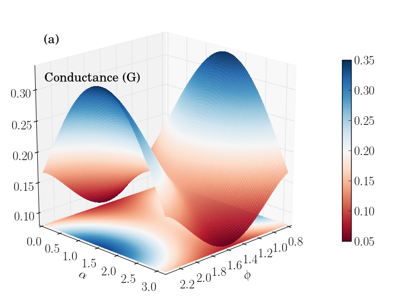
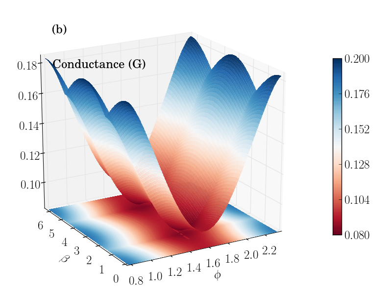
Figure 4: In Fig. (4a), the tunneling conductance $G$ (normalised to unity at $\phi=\tan^{-1}a$) is plotted as a function of the polar angle $\alpha$ of the tip and $\phi$, the angle that spans the surface, for fixed azimuthal angle $\beta=0$, fixed curvature $a=1$ and fixed sharpness parameter $R=1$. In Fig. (4b), the tunneling conductance $G$ is plotted as a function of the azimuthal angle $\beta$ and $\phi$, for fixed polar angle $\alpha=0.1$ for the same curvature and sharpness.

IV Discussion and conclusion

Although we have restricted ourselves to concave hyperbolae for the above calculations, they can be extended to cases where the convex side is filled with the TI. As explained in Ref.takane , in this case, $r<0$. But the Jacobian becomes ill-defined when $|r|\gtrsim R$ due to the presence of the term $(-|r|+f)^{-1}$. Hence, we need to restrict ourselves to $|r|\lesssim R$. In that case, a very similar analysis works and the surface is described by the effective Hamiltonian in Eq.34 with the difference that now $\tilde{\mathcal{A}}_{\phi}=\left[A_{\phi}-m_{2}\langle(-|r|+f)^{-1}\rangle\right]\left(\partial_{\phi}\tilde{\phi}\right)$. The sign change compared with the earlier case implies that the velocity of the electrons is now reduced, and hence its amplitude and consequently, the DOS shows peaking at the corners instead of dips. This can also be measured by an STM tip.

In conclusion, we have found the effective Hamiltonian on curved hyperbolic surfaces and shown that the Hamiltonian can be written in terms of a continuous coordinate which varies along the surface. This clearly indicates that there is no back-scattering for any curvature. The sharpness of the edge can also be changed continuously with no backscattering even at sharp edges. However, the DOS does change as we span the surface and there is a dip (or peaking) of the DOS at the edge for concave (convex) surfaces. We have also shown that the STM spectra of the Dirac electrons on the curved surface, as measured by a magnetized tip, shows unconventional and non-trivial dependence, not only on the parameter spanning the surface, but also on the polar and azimuthal angles of the tip. These measurements would provide clear evidence for the curvature of the surface.

References

- (1)
- (2) C. L. Kane and E. J. Mele, Phys. Rev. Lett. 95, 226801 (2005); ibid, Phys. Rev. Lett. 95, 146802 (2005); C. Wu, B. A. Bernevig, and S. C. Zhang, Phys. Rev. Lett. 96, 106401 (2006); B. A. Bernevig, T. L. Hughes, and S. C. Zhang, Science 314, 1757 (2006); J. E. Moore and L. Balents, Phys. Rev. B75, 121306 (2007); R. Roy, Phys. Rev. B79, 195321 (2009).
- (3) König, M., H. Buhmann, L. W. Molenkamp, T. L. Hughes, C.-X. Liu, X. L. Qi, and S. C. Zhang, J. Phys. Soc. Jpn. 77, 031007(2008); König, M., S. Wiedmann, C. Brune, A. Roth, H. Buhmann, L. Molenkamp, X.-L. Qi, and S.-C. Zhang, Science 318, 766 (2007).
- (4) M. Buttiker, Science 325, 278 (2009); M. Z. Hasan and C. L. Kane, Rev.Mod.Phys. 82, 3045 (2010), X-L Qi and S-C Zhang, Rev. Mod. Phys. 83, 1057 (2011).
- (5) See, for instance, O. Heinonen, ‘Composite fermions: a unified view of the quantum Hall regime’, World Scientific, Singapore (1998).
- (6) C. -Y. Hou, E. -A. Kim, and C. Chamon, Phys. Rev. Lett. 102, 076602 (2009) ; J. Maciejko, C. Liu, Y. Oreg, X. -L. Qi, C. Wu, and S. C. Zhang, Phys. Rev. Lett.102, 256803 (2009) ; A. Ström and H. Johannesson, Phys. Rev. Lett. 102, 096806 (2009) ; A. Bermudez, D. Patane, L. Amico, M. A. Martin-Delgado, Phys. Rev. Lett. 102, 135702 (2009) ; J. E. Moore, Nature 464, 194 (2010); N. Goldman, I. Satija, P. Nikolic, A. Bermudez, M. A. Martin-Delgado, M. Lewenstein, I. B. Spielman, Phys. Rev. Lett. 105, 255302 (2010) ; R. Egger, A. Zazunov and A. Levy Yeyati, Phys. Rev. Lett. 105, 136403 (2010); Joseph Maciejko, Eun-Ah Kim and Xiao-Liang Qi, Phys. Rev. B 82, 195409 (2010); J. E. Vayrynen and T. Ojanen. Phys. Rev. Lett. 106, 076803 (2011); P. Virtanen and P. Recher, Phys. Rev. B 83, 115322 (2011).
- (7) S. Das and S. Rao, Phys. Rev. Lett. 106, 236403 (2011).
- (8) A. Soori, S. Das and S. Rao, Phys. Rev.B 86, 125312 (2012).
- (9) T. Zhang, P. Cheng, X. Chen, J. Jia, X. Ma, K. He, L. Wang, H. Zhang, X. Dai, Z. Fang, X. Xie, and Q. Xue, Phys. Rev. Lett. 103, 266803 (2009).
- (10) P. Roushan, J. Seo, C. V. Parker, Y. S. Hor, D. Hsieh, D. Qian, A. Richardella, M. Z. Hasan, R. J. Cava and A. Yazdani, Nature 460, 1106 (2009).
- (11) J. Seo, P. Roushan, H. Beidennkopf, Y.S. Hor, R. J. Cava and A. Yazdani, Nature 466, 343 (2010).
- (12) K. Imura, Y. Takane and A. Tanaka, Phys. Rev. B84, 195406 (2011).
- (13) K. Imura, Y. Yoshimura, Y. Takane and T. Kukui, cond-mat/1205.4878.
- (14) K. Imura and Y. Takane, cond-mat/1211.2088.
- (15) B. Zhou, H. Lu, R. Chu, S. Shen, and Q. Niu, Phys. Rev. Lett. 101, 246807 (2008).
- (16) Y. Jiang, F. Lu, F. Zhai, T. Low and J. Hu, Phys. Rev. B84, 165439 (2011).
- (17) R. Takahashi and S. Murukami, Phys. Rev. Lett. 107, 166805 (2011).
- (18) D. Sen and O. Deb, Phys. Rev. B85, 245402 (2012); S. Modak, K. Sengupta and D. Sen, cond-mat/1203.4266.
- (19) K. Saha, S. Das, K. Sengupta and D. Sen, Phys. Rev. B 84, 165439 (2011).
- (20) Y. Takane and K. Imura, J. Phys. Soc. Jpn, 81, 093705, (2012).
- (21) H. Zhang, C. Liu, X. Qi, X. Dai, Z. Fang and S. C. Zhang, Nature Physics 5, 438 (2009).
- (22) J. Bardeen, Phys. Rev. Lett. 6, 57 (1961).