Numerical construction of a low-energy effective Hamiltonian in a self-consistent Bogoliubov-de Gennes approach of superconductivity
Abstract
We propose a fast and efficient approach for solving the Bogoliubov-de Gennes (BdG) equations in superconductivity, with a numerical matrix-size reduction procedure proposed by Sakurai and Sugiura [J. Comput. Appl. Math. 159 (2003) 119]. The resultant small-size Hamiltonian contains the information of the original BdG Hamiltonian in a given low-energy domain. Thus, the present approach leads to a numerical construction of a low-energy effective theory in superconductivity. The combination with the polynomial expansion method allows a self-consistent calculation of the BdG equations. Through numerical calculations of quasi-particle excitations in a vortex lattice, thermal conductivity, and nuclear magnetic relaxation rate, we show that our approach is suitable for evaluating physical quantities in a large-size superconductor and a nano-scale superconducting device, with the mean-field superconducting theory.
1 Introduction
To solve an eigenvalue equation is one of the central issues in condensed matter physics. The ground state in a many-body system is nothing but the eigenvector associated with the lowest eigenvalue of a many-body Hamiltonian. The Lanczos algorithm in the exact diagonalization [1] is suitable for this issue. The critical temperature in superconductivity is evaluated by the greatest eigenvalue of the linearized Eliashberg equations. The power iteration algorithm is useful for solving these equations. Thus, a lot of efficient methods for either minimum or maximum eigenvalues have been developed.
In superconductors, low-energy quasiparticle excitations are quite important for examining thermodynamic quantities, transport properties, and so on. Their energy scale is characterized by a superconducting gap energy (), much smaller than a band width (). In the mean-field Bardeen-Cooper-Schrieffer (BCS) theory, these excitations correspond to the eigenvalues at the center of an energy distribution of the Bogoliubov-de Gennes (BdG) Hamiltonian[2]. This is a direct consequence of the particle-hole symmetry of the BdG Hamiltonian. Furthermore, such an intermediate region can include zero eigenvalues (i.e., zero modes). The zero modes are related to fundamental properties of topological insulators and superconductors [3]. Therefore, in order to study bulk properties of various superconductors and nano-scale devices with topological materials from atomic-scale physics, an efficient method to obtain an intermediate spectral region of the BdG Hamiltonian is highly desirable.
Typically, the full diagonalization method is used for solving the BdG equations [4, 5, 6, 7]. However, this approach requires a lot of computational memories and a long computational time. In contrast, the polynomial expansion method [8, 9, 10, 11, 12] allows efficient self-consistent calculations in superconductivity, without any diagonalization. This approach drastically reduces a computational cost and has an excellent parallel efficiency, but does not lead to direct calculations of eigen-pairs (eigenvalues and eigenvectors) of the BdG Hamiltonian. Thus, this method is not suitable for calculating dynamical correlation functions (two-particle Green’s functions), which lead to important quantities such as spin/charge susceptibilities, nuclear magnetic relaxation rate, optical/thermal conductivities. Hence, the algorithms for treating an intermediate energy region of the BdG Hamiltonian have not been adequately studied.
In this paper, we propose a fast and efficient method for numerically calculating the eigenvalues and the eigenvectors of the BdG equations. Our approach is the combination of the polynomial expansion method with a contour-integral-based method developed by one of the present authors (TS) and Sugiura (Sakurai-Sugiura method)[13, 14, 15, 16]. The Sakurai-Sugiura (SS) method allows us to extract the eigen-pairs whose eigenvalues are located in a given domain on the complex plane, from a generic matrix. Therefore, setting this domain around the origin of , an effective Hamiltonian for the full BdG Hamiltonian can be constructed, with keeping the information relevant to low-energy excitations in a superconductor. A contour-integral representation of the projection operator onto an energy domain plays a crucial role. We obtain an effective Hamiltonian only with a gapless surface state in topological insulators and superconductors in large-scale systems, for example.
Let us summarize our approach for calculating physical quantities in the mean-field superconducting theory. First, we perform a self-consistent calculation of the BdG equations to obtain a superconducting gap function. Next, we numerically derive a low-energy (small-size) effective Hamiltonian from the BdG Hamiltonian with the resultant superconducting gap. Finally, we calculate physical quantities using the eigenvalues and the eigenvectors of this effective Hamiltonian.
This paper is organized as follows. In Sec. 2, we show a general formulation of a mean-field fermionic theory. The Green’s functions are expressed by the eigenvalues and the eigenvectors of the BdG equations. In Sec. 3, we explain the polynomial expansion scheme. The application of the SS method to superconductivity is proposed in Sec. 4. We show the theoretical background of this approach and the algorithm. We stress that the present algorithm is suitable for parallel computation since the procedure is composed of solving a set of the linear equations which are independent of each other. In Sec. 5, we show the results for typical examples, as well as the computational costs of the present proposal. We perform large-scale calculations in various physical situations. As for inhomogeneous systems, we consider a vortex lattice on a two-dimensional square lattice. The quasiparticle excitation spectrum is obtained, varying a magnetic field and a coherence length. The thermal conductivity is also evaluated. Moreover, we examine temperature-dependence of the nuclear magnetic relaxation rate in an -wave superconductor, as an example of a uniform superconductor. These demonstrations indicate that the present approach is a fast and accurate method for numerically constructing a low-energy effective Hamiltonian in the mean-field superconducting theory. Section 6 is devoted to the summary.
2 Formulation
2.1 Hamiltonian
Throughout this paper, we set . Let us consider a Hamiltonian for a fermionic many-body system,
| (1) |
with and . Here, the symbol represents transposition. The fermionic annihilation and creation operators are denoted as, respectively, and (). The index includes all the relevant degrees of freedom such as spatial sites, spins, orbitals, and so on. The canonical anti-commutation relation is . The Hamiltonian matrix is a Hermite matrix. The hermitian property of and the canonical anti-commutation relation imply that the complex matrices and in satisfy and . In the case of superconductivity, corresponds to the mean-field BCS Hamiltonian and contains superconducting gaps.
2.2 Bogoliubov-de Gennes equations
The BdG equations are regarded as the eigenvalue equations with respect to
| (2) |
with . The column vectors and are -component complex vectors. To solve the BdG equations is equivalent to the diagonalization of with a unitary matrix . The matrix elements of are
| (3) |
The eigenvalues are not independent of each other. In fact, using the particle-hole transformation [17] such that , one can show that .
2.3 Two-particle Green’s functions
Two-particle Green’s functions are related to different physical quantities in condensed matter physics. Here,they are written in terms of the solutions of the BdG equations. Let us consider a two-particle Green’s function in the imaginary time ,
| (4a) | ||||
| (4b) | ||||
with the one-particle Green’s functions
| (5a) | ||||
| (5b) | ||||
| (5c) | ||||
| (5d) | ||||
With the use of the relation
| (6) |
the Fourier transformed function is
| (7) |
Here, is the inverse temperature and and are the fermionic and bosonic Matsubara frequencies, respectively. The one-particle Green’s functions are written as a matrix,
| (8) |
We find that , , , and . We can phenomenologically describe a dissipation effect, replacing the delta function in with an approximate -function. The dynamical correlation function with the real energy is
| (9) |
with setting () in Eq. (7). Here, denotes the fermion distribution function.
3 Polynomial expansion method
We briefly summarize the polynomial expansion method for a self-consistent calculation of the BdG equations, according to our previous paper[11]. The essence is the expansion of the spectral density of the Green’s functions, with orthonormal polynomials in satisfying
| (10a) | |||
| (10b) | |||
| (10c) | |||
The Chebyshev polynomial is often used, because the resultant formulae become the simplest forms. The application of the other polynomials is discussed in, e.g., our previous paper [18].
The spectral density (matrix) is given as a difference between the retarded and the advanced Green’s functions, . Let us expand by , rescaling and so that and , with and . Here, and are energy scales satisfying . The elements of are related to various correlation functions. Using the constant vectors and such that and , we obtain
| (11a) | ||||
| (11b) | ||||
where
| (12) |
A sequence of a vector [] is recursively obtained by
| (13a) | ||||
| (13b) | ||||
The use of the recurrence formula leads to a self-consistent calculation of the BdG equations, without any diagonalization of .
4 Contor-integral-based method (Sakurai-Sugiura method)
In this paper, we use the SS method for finding eigenvalues in a given energy domain and their associated eigenvectors. This approach is a numerical solver for a generalized eigenvalue problem so that , with , and has been applied to various physical issues such as the real-space density functional theory[19] and the lattice quantum chromodynamics[20]. In this paper, is the identity matrix, and is an Hermite matrix.
Our aim is to reduce the size of , keeping as much information of the eigenvalues and the eigenvectors as possible. Let us consider the use of an () matrix , whose th column is (i.e., ). Here is a set of linearly independent vectors in . We obtain an matrix
| (14) |
We denote a given energy domain of as . Let us suppose that is represented by a linear combination of , where (). Thus, contains eigenvalues of (). It is necessary for implementing this procedure to know parts of the eigenvectors of . Furthermore, one has to carefully choose to avoid losing the relevant information of . Remarkably, this issue will be solved by an approximate evaluation of contour integrals associated with a projection operator onto eigenspaces of . All the steps of the algorithm is summarized in Sec. 4.4.
4.1 Projection and moment vectors
We start with a way to make a projection onto a target subspace spanned by (). An arbitrary -dimensional vector is expanded by , with complex coefficients, . We define the projection as
| (15) |
Using , we find that the resolvent[21] of is
| (16) |
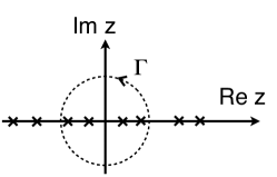
with the identity matrix, and a set of all the eigenvalues of , , since . Let us suppose that the distinct eigenvalues (i.e., simple poles on ) are located inside a closed loop on , and the others are outside , as shown in Fig. 1. Thus, we obtain a contour-integral representation of
| (17) |
Now, let us write essential quantities for determining the reduction matrix . The moment vector () is defined as , with a vector . From its contour-integral representation, we find that is related to the th moment,
| (18) |
An important property of is that this is a vector in a vector space associated with . This fact is checked by applying to Eq. (15). We remark that all the moment vectors are linearly independent of each other for an arbitrary , since the subspace spanned by is the order- Krylov subspace[22] generated by , . In our algorithm to determine , is an input parameter. Then, one has to construct linearly independent vectors from , varying , and evaluate with a proper manner. Another important issue is to numerically calculate the contour integrals. These points will be explained in the following.
4.2 Approximation of contour integrals with numerical quadrature
We show a method to approximate a contour integral with numerical quadrature. Let us suppose that a Jordan curve on is represented by scaling and shifting another Jordan curve , with a scaling factor and a shift . Without loss of generality, we assume that encloses the origin on . Let be a point on , with a parameter (), and let on be given by . Then, using -point quadrature rule, the moment vector is approximately written by
| (19) |
with , , , and . The vector is the solution of the linear equation . When all the eigenvalues are located on the real axis, it might be better to put the quadrature points closer to the real axis,
| (20) |
with vertical scaling factor (). The quadrature weight is
| (21) |
When , is a unit circle. Other formulae including contour integrals are also calculated by this -point numerical quadrature.
4.3 Construction of subspace
Now, we show a way to determine the subspace size and the corresponding reduction matrix. First, we make a sequence of the moment vectors, varying . The use of this sequence is essential for constructing the linearly independent vectors and the subspace. We set complex vectors, (), and make an real matrix . We call a source matrix. Then, we obtain an matrix ,
| (22) |
with
| (23) |
The th column of is related to , , with . Each element of is a uniform random variable in . It means that we make via random sampling, with the source size . The integer parameter is determined by the calculation of , as seen below.
Next, we determine the subspace size. A bundle of leads to an matrix . Now, we perform the singular-value decomposition of , and obtain the singular values , with . Then, we find the number of the singular values satisfying , with a small positive constant . Thus, we have an effective rank (i.e., the number of the predominant linearly independent vectors) of . We stress that this rank should be greater than or equal to a prior value , which is determined by calculating the trace of the resolvent matrix (see below). We use the resultant effective rank as the dimension of the subspace. We remark a large source size leads to a highly accurate calculation, but causes an extreme increase in the subspace size. To avoid this increase for the high accuracy, one can use an iterative refinement[14] of a subspace, as seen in Appendix A.
Now, the construction of the reduction matrix to the subspace is straightforward. Using a submatrix composed of the first columns of (e.g., in terms of Fortran 90) and the Gram-Schmidt orthonormalization, we obtain an matrix whose column vectors are orthonormal to each other. This is our reduction matrix. From the construction manner, one finds that contains predominant eigenvectors of . Alternatively, one may use a matrix such that and . This matrix is automatically obtained when performing the singular-value decomposition of by using the ZGESVD routine of LAPACK, and the column-vectors are orthogonal to each other.
The source size and the moment size have to be carefully chosen. In particular, the integer , which is the total number of the moment vectors to take in a simulation, should be as small as possible for a few computational costs. First, we predict the prior rank , with the stochastic estimation method[15, 16]. We prepare an real matrix whose elements are either or with equal probability. Here, is an input parameter. The number of the eigenvalues inside is , since
| (24) | ||||
| (25) |
The stochastic estimation of for an matrix is (See, Appendix B). Thus, using the -point numerical quadrature, is estimated by
| (26) |
Then, the source size is
| (27) |
with . The symbol means the smallest integer greater than . The value of is larger than . Thus, the requirement that the rank of is greater than and equal to is automatically satisfied.
4.4 Algorithm of the SS method
Now, we show all the steps of the SS method for calculating the eigenvalues and the eigenvectors of the BdG Hamiltonian .
(i) Set (), , , and . The elements of the sampling vector take either -1 or 1, with equal probability.
(ii) Solve Eq. (23) for . One can solve these equations separately so that parallel computations can be easily implemented.
(iii) Compute Eq. (22).
(v) Give the elements of by random numbers and solve Eq. (23).
(vi) Compute Eq. (22) using the results in (v).
(vii) Perform the singular-value decomposition and find such that for .
(viii) Obtain a matrix from .
(ix) Form .
(x) Compute the eigenvalues and eigenvectors of the matrix .
(xi) Set .
5 Numerical demonstrations
We show the effectiveness and the validity of the present approach, focusing on a single-band superconductor. Hereafter, the index in Sec. 2.1 indicates a spatial site on a two-dimensional square lattice. The spin indices ( and ) are explicitly written in the creation and annihilation operators. We consider a two-dimensional lattice system, with the nearest-neighbor hopping . The spatial site index runs from to . We impose the periodic boundary condition. The superconducting gap equations is given as , with pairing interaction . This equation is self-consistently solved by the polynomial expansion method, as shown in Sec. 3. The parameters in the SS method are set as , and . We remove the eigen-pair whose relative residual is greater than , as spurious eigenpairs. See Eq. (28). We do not use the iterative refinement of a subspace in the following examples.
5.1 Computational costs in self-consistent calculations
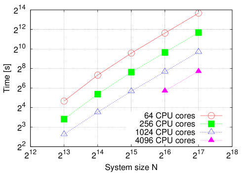
We use the polynomial expansion scheme to obtain self-consistent superconducting gaps. Let us evaluate computational costs for a -wave superconductor at zero temperature, on a square lattice (). An evaluation for an -wave superconductor was shown in our previous contribution [11]. We measure the elapsed time for calculating and updating the order parameters at one iteration.
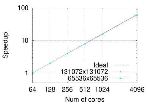
We used a supercomputing system PRIMERGY BX900 in Japan Atomic Energy Agency. As shown in Fig. 2, the elapsed time for one iteration is subjected to an rule, with increasing the system size . This tendency is kept from 32 to 4096 CPU cores. In contrast, the full diagonalization scheme inevitably demands costs in the core part of a calculation. This is a big advantage of the polynomial expansion scheme. Furthermore, we focus on the strong scaling, as shown in Fig. 3. One can see an excellent strong scaling up to 4096 CPU cores.
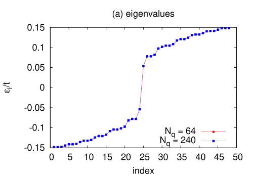
5.2 Eigenvalues in a vortex lattice system in an -wave superconductor
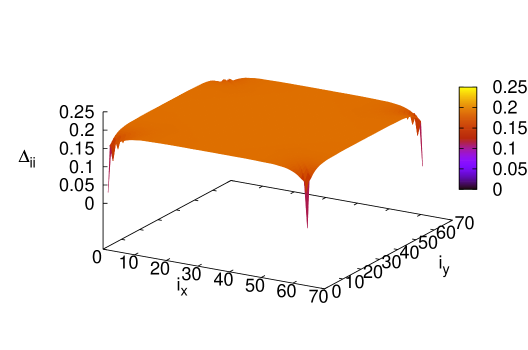
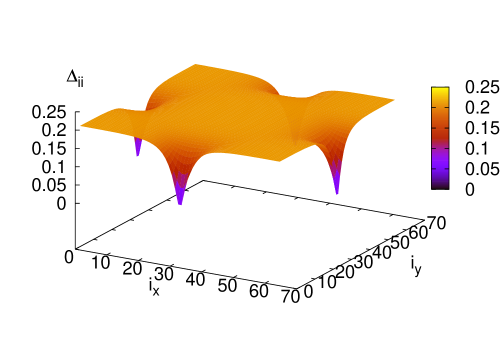
We show the eigenvalues obtained by the SS method. The system in this section has a vortex square lattice in an -wave superconductor. The parameters are set as follows: on-site interaction , chemical potential , and spatial size . The matrix dimension is with 49152 nonzero entries. The rescaling parameters in the polynomial expansion method are and . Also, a cut-off parameter in the polynomial expansion scheme[11] is . The resultant order parameter is shown in Fig. 4.
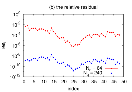
The relative residual for the eigen-pair is calculated by
| (28) |
After the self-consistent calculations with 100 iterations, we obtain the eigen-pairs with the use of the SS method.
The quadrature points are set by Eq. (20) and the corresponding weights are set by Eq. (21), with . The contour is set as and . We adopt a sparse solver PARDISO[23] to compute Eq. (23). This solver uses the nested dissection algorithm from the METIS package[24]. We also confirm that the calculations with the shifted BiCG method, which is suitable for large sparse matrices, have a similar result.
Let us investigate -dependence of the eigenvalues and the relative residual. Figure 5 shows that a calculation with has good precision about the eigenvalues inside (). We note that the calculation with takes about 30 seconds with only one CPU core (Intel Xeon X5550 2.66GHz) by a desktop computer. The conventional full diagonalization takes about 40 minutes with the same machine. When the system size becomes quadruple (), it takes about 5 minutes to obtain the same eigenvalue distribution, with the same one CPU core.
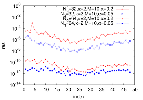
We discuss the accuracy of an eigenvalue calculation in the SS method. This issue depends on the parameters related to the contour integral representation, as well as the source size . The simplest improvement can be achieved by increasing the total number of the quadrature points, . Alternatively, we obtain better accuracy with smaller , continuously deforming the contour . Figure 6 shows the relative residual, varying and the vertical scaling factor . We find that the accuracy becomes higher than Fig. 5(b), even though is small. Here, we take a relatively larger source size ( and in Eq. (27)), compared with the previous calculations.
|
|
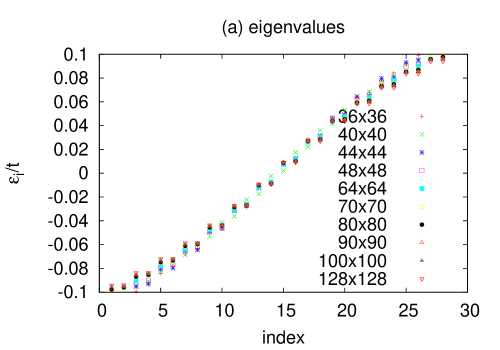
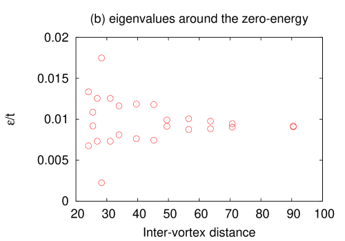
5.3 Magnetic-field dependence of the eigenvalue in long-coherence-length superconductors
We show the magnetic-field dependence of the eigenvalues in a long-coherence-length superconductor. A coherence length of a superconductor is roughly estimated by the ratio of the Fermi velocity to the amplitude of the order-parameter (). In many materials expect for high- cuprates, the coherence length is much larger than an atomic length. Typically, the electric states in such superconducting systems are described by the quasiclassical Eilenberger theory[25], with neglecting atomic-scale physics. However, interesting microscopic phenomena such as an interference effect and discretized quantum bound states in a vortex core are never treated in this approach. The mean-field BdG approach can treat these atomic-scale phenomena, but requires extremely large computational costs when the coherence length is much larger than an atomic length. Thus, to solve the BdG equations in a long-coherence-length superconductor is a challenging issue.
We consider a vortex lattice in an -wave superconductor, with on-site interaction and chemical potential . These parameters correspond to a model with a relatively smaller Fermi surface, compared with Sec. 5.2. The temperature is set as . We use the domain with and (), and . The magnetic field becomes small with decreasing the system size, since the total magnetic flux is fixed. As shown in Fig. 7, the amplitude of the order-parameter is similar to that in the previous section. Combined with the small Fermi surface, the coherence length is longer than in Sec. VB. Under the periodic boundary condition, two bound states appear at each vortex core. Their energy eigenvalues are degenerate when the system size is large (low magnetic field). With increasing the magnetic field, a splitting in the degenerate eigenvalues occurs, as shown in Fig, 8(a). The splitting comes from the occurrence of an overlap between the bound states in a vortex core. Figure 8(b) shows quantum oscillation as a function of the inter-vortex distance originating from an interference effect between two vortex bound states. We note that it is hard to discuss the degeneracy splitting with the only use of the polynomial expansion scheme, since the polynomial expansion calculates the local density of the states not the eigenvalues.
|
|
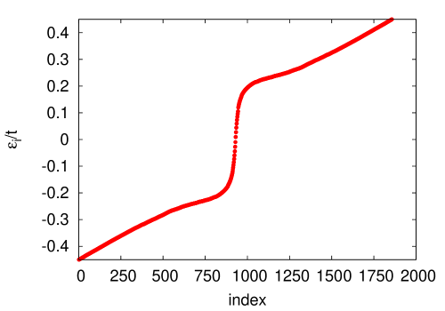
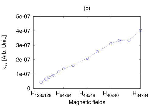
5.4 Magnetic field dependence of the thermal conductivity
We show the magnetic-field-dependence of the thermal conductivity in an -wave superconductor, with a vortex lattice. All the physical parameters are the same as the ones in Sec. 5.3. We use the domain with and (), and . It takes about one hour to obtain 1857 eigenvalues located in the domain with the same one CPU core when the system size is as shown in Fig. 9. One can clearly find that the gap amplitude in the bulk states is , which is consistent with the estimation with the use of Fig. 7.
Let us consider the case when a temperature gradient exists along -axis. Using the linear response theory [26], the electronic thermal conductivity per volume of a superconductor is
| (29) | |||||
| (30) |
with
| (31) | |||||
Here, is the Fourier transformation of a current-current correlation function [27, 28, 5] in the imaginary time, , where is the Heisenberg operator of energy flux[27] along -axis. The Lorentian kernel in represents a dissipation effect [5]. The matrix contains the eigenvectors of the BdG Hamiltonian, while the matrix includes contributions from the energy flux. We show their explicit formulae in Appendix C.
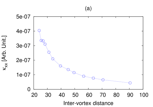
We adopt the damping factor . We assume that in Eq. (41) because the vector potential around a vortex is small. Figure 10 shows that drastically increases when the inter-vortex distance is shorter than around 60 (i.e., a high magnetic-field domain). This behavior could be related to an interference effect between the two bound states in vortex cores in high magnetic field, as seen Fig. 7. A quantum oscillation in the eigenvalue distribution becomes remarkable in such a high magnetic-field domain.
|
|
5.5 Temperature dependence of nuclear magnetic relaxation rates
We show the temperature dependence of the nuclear magnetic relaxation rate in a uniform -wave superconductor. It is well known that the nuclear magnetic relaxation rate is calculated by[4]
| (32) | ||||
| (33) | ||||
| (34) |
We use the eigenvalues in the domain with , (). The parameters are set as follows: the onsite interaction , the chemical potential , and the system size . The delta function is approximated by with the smearing factor . We adopt the shifted BiCG method as a iterative linear solver.
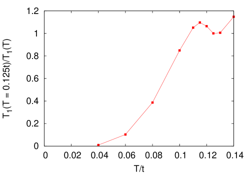
As shown in Fig. 11, the nuclear magnetic relaxation rate can be successfully reproduced by the SS method. We note that the discrete energy levels due to the finite size system cause the relatively smaller Hebel-Slichter peak below . We mention here that the accuracy of calculating physical quantities by the SS method depends on the size of an energy domain on the complex plain. A truncation error may occur in evaluating Eq. (9), if this size is not enough large. Figure 6 indicates the eigen-pairs inside are evaluated with high accuracy. Therefore, the accuracy of evaluating the nuclear magnetic relaxation rate around may increase, taking a relatively larger domain size.
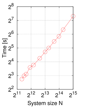
5.6 Computational costs in the eigenvalue problem with the SS-method in a vortex lattice system
Now, let us evaluate the computational costs of the SS method. We measure the elapsed time from reading the Hamiltonian matrix constructed by the polynomial expansion scheme to finishing the SS-method in a square lattice -wave superconductor at (). We use the contour with and , and the physical parameters are the same as in Fig. 8. For the measurement, we use a desktop computer with only one CPU core (Intel Xeon X5550 2.66GHz). As shown in Fig. 12, the elapsed time of the SS method grows in an manner with increasing the system size . The computational costs are roughly estimated by . In all the calculation of this subsection, the energy domain is restricted to . As a result, the number of the eigenvalues is independent of the spatial size . Indeed, we find that only the bound states in vortices are relevant to this narrow energy window. If an energy domain is wide (large ), increases. In this case, the computational cost predominantly depends on the Gram-Schmidt orthonormalization procedure to construct . Then, we find that the cost is estimated by . When one tries to obtain all the eigenvalues (i.e., ) with a wide energy domain, the cost of the SS method becomes . This result is equivalent to the one in the full diagonalization method. However, the wide energy domain is easily divided into small energy domains. For example, with using domains with parallel computation with CPU cores, the elapsed time reduces to . This is a big advantage of the SS method.
6 Conclusion
We proposed the fast efficient method on the basis of the SS-method and the polynomial expansion scheme to calculate the eigen-pairs and the dynamical correlation functions in the BdG scheme of superconductivity. The polynomial expansion scheme enables us to solve the gap-equations self consistently, with large scale parallel computations. With the use of the SS method, one can solve issues for finding eigenvalues in a given energy domain and their corresponding eigenvectors. The virtue of the SS method is to reduce systematically the size of a large Hamiltonian, keeping its predominant contributions in a low-energy scale. In other words, this proposal leads to a numerical construction of an effective low-energy Hamiltonian in the BdG approach of superconductivity. We applied the present approach to the calculations of various physical quantities including the eigenvalues distribution of the BdG Hamiltonian in a vortex lattice, magnetic-field-dependence of the thermal conductivity, and temperature-dependence of the nuclear magnetic relaxation rate. We stress that most of the calculations were performed, changing the system size. This is quite important for developing a theoretical tool to predict physical behaviors in nano-scale superconductors from a microscopic theory.
The authors would like to acknowledge Masahiko Machida and Susumu Yamada for helpful discussions and comments. The calculations have been performed using the supercomputing system PRIMERGY BX900 at the Japan Atomic Energy Agency. This study has been supported by Grants-in-Aid for Scientific Research from MEXT of Japan. Y.O. is supported in part by the Special Postdoctoral Researchers Program, RIKEN.
Appendix A Iterative refinement
In Sec. 4.3, we remark that larger subspace makes more higher accuracy but needs more heavier computational costs. A problem may occur when we choose a small value of to avoid the use of a large subspace. If some residuals of the obtained approximate eigenvalues and eigenvectors are not small enough for a given tolerance, we can brush up the resulting approximate eigenvalues and eigenvectors. We propose two ways to brush up the eigen pairs with the choice of the appropriate source matrix dominantly constructed by the information in a given domain .
First, one can use the source matrix as
| (35) |
Then, we implement iterations of on ,
| (36) |
Using , we construct a refined matrix including a higher moment vector, . In a simulation, numerical quadrature is used for calculating and , as seen in Sec. 4.2. Thus, performing the singular-value decomposition of , we evaluate a refined effective rank .
Second, we can brush up the resulting approximate eigenvalues and eigenvectors by setting the source matrix as
| (37) |
where whose elements are random numbers in , and are the selected eigenvectors that are regarded as the approximate eigenvectors with respect to the eigenvalues inside . Using this , we reevaluate and in Sec. 4.2.
Appendix B Estimation of the trace
We show that the trace of an matrix can be estimated by
| (38) |
with random vectors with entries . If the vectors have entries , the right-hand side in the above equation is expressed as
| (39) |
On the average, the coefficient of in the above expansion will converge to zero provided that the components of the vectors have balanced signs.
Appendix C Thermal conductivity
We derive the expression of the thermal conductivity in terms of the solution of the BdG equation. Let us consider the case when a temperature gradient exists along -axis on a two-dimensional lattice with lattice constant . The electronic thermal conductivity per volume of a superconductor associated with heat flux along -axis is given in Eq. (29). The current-current correlation function with respect to the energy flux is
| (40) |
The Heisenberg operator of energy flux [27] along -axis is
| (41) |
with and . The link variable represents the contribution of the magnetic field, , with the flux quantum and the vector potential . The matrix is related to the momentum operator on a square lattice [5].
This current-current correlation function may be rewritten as the form of a two-particle Green’s function [28],
| (42) | |||||
with and . We neglected some terms associated with the action of the imaginary-time derivative on the time ordering operator, according to the discussion by Ambegaokar and Teword [28]. Here, and are defined as, respectively, and , with and . This convention corresponds to the Nambu representation. The indices , , , and run from to . The matrix is defined as
| (43) |
with the matrix . The formulation in Sec. 2, which is developed in a more general representation for a fermion mean-field theory, is straightforwardly rewritten in terms of the Nambu representation.
References
- [1] E. Dagotto: Rev. Mod. Phys. 66 (1994) 763.
- [2] P. G. de Gennes, Superconductivity of Metals and Alloys (Westview Press, Boulder, CO, 2008).
- [3] J. C. Y. Teo and C. L. Kane: Phys. Rev. B 82 (2010) 115120.
- [4] M. Takigawa, M. Ichioka and K. Machida: J. Phys. Soc. Jpn. 69 (2000) 3943.
- [5] M. Takigawa, M. Ichioka, and K. Machida: Eur. Phys. J. B 27 (2002) 303.
- [6] B. M. Andersen, P. J. Hirschfeld, A. P. Kampf, and M. Schmid: Phys. Rev. Lett. 99 (2007) 147002.
- [7] B. M. Andersen and P. J. Hirschfeld: Phys. Rev. Lett. 100 (2008) 257003.
- [8] L. Covaci, F. M. Peeters and M. Berciu: Phys. Rev. Lett. 105 (2010) 167006.
- [9] G. Q. Zha, L. Covaci, S. P. Zhou, and F. M. Peeters: Phys. Rev. B 82 (2010) 140502(R).
- [10] Q. Han, T. Li, and Z. D. Wang: Phys. Rev. B 82 (2010) 052503.
- [11] Y. Nagai, Y. Ota, and M. Machida: J. Phys. Soc. Jpn. 81 (2012) 024710.
- [12] Y. Nagai, N. Nakai, and M. Machida: Phys. Rev. B 85 (2012) 092505.
- [13] T. Sakurai and H. Sugiura: J. Comput. Appl. Math. 159 (2002) 119.
- [14] T. Sakurai, Y. Futamura, and H. Tadano: to be published in J.of Algo. & Comp. Tech.
- [15] Y. Futamura, H. Tadano, and T. Sakurai: JSIAM Lett. 2 (2010) 127.
- [16] Y. Maeda, Y. Futamura, T. Sakurai: JSIAM Lett. 3 (2011) 61.
- [17] J. L. van Hemmen: Z. Phys. B 38 (1980) 271.
- [18] Y. Nagai, Y. Ota, and M. Machida: Physics Procedia 27 (2012) 72.
- [19] Y. Futamura, T. Sakurai, S. Furuya, and J.-I. Iwata: High Performance Computing for Computational Science –VECPAR 2012, Lecture Notes in Computer Science (accepted).
- [20] H. Ohno, Y. Kuramashi, T. Sakurai, and H. Tadano: JSIAM Letters, 2 (2010) 115.
- [21] A. Messiah, Quantum Mechanics: Two Volumes Bound as One (Dover, New York, 1999), pp.712-714.
- [22] D. S. Watkins, The Matrix Eigenvalue Problem: GR and Krylov Subspace Methods (SIAM, Philadelphia, 2008), Chap.9.
- [23] O.Schenk and K.Gartner: J. of Future Generation Computer Systems, 20 (2004) 475.
- [24] G. Karypis and V. Kumar: SIAM Journal on Scientific Computing, 20 (1998) 359.
- [25] G. Eilenberger: Z. Phys. 214 (1968) 195.
- [26] R. Kubo, M. Yokota, and S. Nakajima: J. Phys. Soc. Jpn. 12 (1957) 1203.
- [27] J. S. Langer: Phys. Rev. 128 (1962) 110.
- [28] V. Ambegaokar and L. Teword: Phys. Rev. 134 (1964) A805.