Topic Discovery through Data Dependent and Random Projections

Abstract

We present algorithms for topic modeling based on the geometry of cross-document word-frequency patterns. This perspective gains significance under the so called separability condition. This is a condition on existence of novel-words that are unique to each topic. We present a suite of highly efficient algorithms based on data-dependent and random projections of word-frequency patterns to identify novel words and associated topics. We will also discuss the statistical guarantees of the data-dependent projections method based on two mild assumptions on the prior density of topic document matrix. Our key insight here is that the maximum and minimum values of cross-document frequency patterns projected along any direction are associated with novel words. While our sample complexity bounds for topic recovery are similar to the state-of-art, the computational complexity of our random projection scheme scales linearly with the number of documents and the number of words per document. We present several experiments on synthetic and real-world datasets to demonstrate qualitative and quantitative merits of our scheme.

1 Introduction

We consider a corpus of $M$ documents composed of words chosen from a vocabulary of $W$ distinct words indexed by $w=1,\ldots,W$. We adopt the classic “bags of words” modeling paradigm widely-used in probabilistic topic modeling (Blei, 2012). Each document is modeled as being generated by $N$ independent and identically distributed (iid) drawings of words from an unknown $W\times 1$ document word-distribution vector. Each document word-distribution vector is itself modeled as an unknown probabilistic mixture of $K<\min(M,W)$ unknown $W\times 1$ latent topic word-distribution vectors that are shared among the $M$ documents in the corpus. Documents are generated independently. For future reference, we adopt the following notation. We denote by ${\bm{\beta}}$ the unknown $W\times K$ topic-matrix whose columns are the $K$ latent topic word-distribution vectors. ${\bm{\theta}}$ denotes the $K\times M$ weight-matrix whose $M$ columns are the mixing weights over $K$ topics for the $M$ documents. These columns are assumed to be iid samples from a prior distribution. Each column of the $W\times M$ matrix ${\mathbf{A}}={\bm{\beta}}{\bm{\theta}}$ corresponds to a document word-distribution vector. ${\mathbf{X}}$ denotes the observed $W\times M$ word-by-document matrix realization. The $M$ columns of ${\mathbf{X}}$ are the empirical word-frequency vectors of the $M$ documents. Our goal is to estimate the latent topic word-distribution vectors (${\bm{\beta}}$) from the empirical word-frequency vectors of all documents (${\mathbf{X}}$).

A fundamental challenge here is that word-by-document distributions (${\mathbf{A}}$) are unknown and only a realization is available through sampled word frequencies in each document. Another challenge is that even when these distributions are exactly known, the decomposition into the product of topic-matrix, ${\bm{\beta}}$, and topic-document distributions, ${\bm{\theta}}$, which is known as Nonnegative Matrix Factorization (NMF), has been shown to be an $\mathcal{NP}$-hard problem in general. In this paper, we develop computationally efficient algorithms with provable guarantees for estimating ${\bm{\beta}}$ for topic matrices satisfying the separability condition (Donoho & Stodden, 2004; Arora et al., 2012b).

Definition 1.

(Separability) A topic matrix ${\bm{\beta}}\in{\mathbb{R}}^{W\times K}$ is separable if for each topic $k$, there is some word $i$ such that ${\beta}_{i,k}>0$ and ${\beta}_{i,l}=0$, $\forall l\neq k$.

The condition suggests the existence of novel words that are unique to each topic. Our algorithm has three main steps. In the first step, we identify novel words by means of data dependent or random projections. A key insight here is that when each word is associated with a vector consisting of its occurrences across all documents, the novel words correspond to extreme points of the convex hull of these vectors. A highlight of our approach is the identification of novel words based on data-dependent and random projections. Our idea is that whenever a convex object is projected along a random direction, the maximum and minimum values in the projected direction correspond to extreme points of the convex object. While our method identifies novel words with negligible false and miss detections, evidently multiple novel words associated with the same topic can be an issue. To account for this issue, we apply a distance based clustering algorithm to cluster novel words belonging to the same topic. Our final step involves linear regression to estimate topic word frequencies using novel words.

We show that our scheme has a similar sample complexity to that of state-of-art such as (Arora et al., 2012a). On the other hand, the computational complexity of our scheme can scale as small as $\mathcal{O}(\sqrt{M}W+MN)$ for a corpora containing $M$ documents, with an average of $N$ words per document from a vocabulary containing $W$ words. We then present a set of experiments on synthetic and real-world datasets. The results demonstrates qualitative and quantitative superiority of our scheme in comparison to other state-of-art schemes.

2 Related Work

The literature on topic modeling and discovery is extensive. One direction of work is based on solving a nonnegative matrix factorization (NMF) problem. To address the scenario where only the realization $\mathbf{X}$ is known and not ${\mathbf{A}}$, several papers (Lee & Seung, 1999; Donoho & Stodden, 2004; Cichocki et al., 2009; Recht et al., 2012) attempt to minimize a regularized cost function. Nevertheless, this joint optimization is non-convex and suboptimal strategies have been used in this context. Unfortunately, when $N\ll W$ which is often the case, many words do not appear in $\mathbf{X}$ and such methods often fail in these cases.

Latent Dirichlet Allocation (LDA)  (Blei et al., 2003; Blei, 2012) is a statistical approach to topic modeling. In this approach, the columns of ${\bm{\theta}}$ are modeled as iid random drawings from some prior distributions such as Dirichlet. The goal is to compute MAP (maximum aposteriori probability) estimates for the topic matrix. This setup is inherently non-convex and MAP estimates are computed using variational Bayes approximations of the posterior distribution, Gibbs sampling or expectation propagation.

A number of methods with provable guarantees have also been proposed. (Anandkumar et al., 2012) describe a novel method of moments approach. While their algorithm does not impose structural assumption on topic matrix ${\bm{\beta}}$, they require Dirichlet priors for ${\bm{\theta}}$ matrix. One issue is that such priors do not permit certain classes of correlated topics (Blei & Lafferty, 2007; Li & McCallum, 2007). Also their algorithm is not agnostic since it uses parameters of the Dirichlet prior. Furthermore, the algorithm suggested involves finding empirical moments and singular decompositions which can be cumbersome for large matrices.

Our work is closely related to recent work of (Arora et al., 2012b) and (Arora et al., 2012a) with some important differences. In their work, they describe methods with provable guarantees when the topic matrix satisfies the separability condition. Their algorithm discovers novel words from empirical word co-occurrence patterns and then in the second step the topic matrix is estimated. Their key insight is that when each word, $j$, is associated with a $W$ dimensional vector the novel words correspond to extreme points of the convex hull of these vectors. (Arora et al., 2012a) presents combinatorial algorithms to recover novel words with computational complexity scaling as $\mathcal{O}(MN^{2}+W^{2}+WK/\epsilon^{2})$, where $\epsilon$ is the element wise tolerable error of the topic matrix ${\bm{\beta}}$. An important computational remark is that $\epsilon$ often scales with $W$, i.e. probability values in ${\bm{\beta}}$ get small when $W$ is increased, hence one needs smaller $\epsilon$ to safely estimate ${\bm{\beta}}$ when $W$ is too large. The other issue with their method is that empirical estimates of joint probabilities in the word-word co-occurrence matrix can be unreliable, especially when $M$ is not large enough. Finally, their novel word detection algorithm requires linear independence of the extreme points of the convex hull. This can be a serious problem in some datasets where word co-occurrences lie on a low dimensional manifold.

Major Differences: Our work also assumes separability and existence of novel words. We associate each word with a $M$-dimensional vector consisting of the word’s frequency of occurrence in the $M$-documents rather than word co-occurrences as in (Arora et al., 2012b, a). We also show that extreme points of the convex hull of these cross-document frequency patterns are associated with novel words. While these differences appear technical, it has important consequences. In several experiments our approach appears to significantly outperform (Arora et al., 2012a) and mirror performance of more conventional methods such as LDA (Griffiths & Steyvers, 2004). Furthermore, our approach can deal with degenerate cases found in some image datasets where the data vectors can lie on a lower dimensional manifold than the number of topics. At a conceptual level our approach appears to hinge on distinct cross-document support patterns of novel words belonging to different topics. This is typically robust to sampling fluctuations when support patterns are distinct in comparison to word co-occurrences statistics of the corpora. Our approach also differs algorithmically. We develop novel algorithms based on data-dependent and random projections to find extreme points efficiently with computational complexity scaling as $\mathcal{O}(MN+\sqrt{M}W)$ for the random scheme.

Organization: We illustrate the motivating Topic Geometry in Section 3. We then present our three-step algorithm in Section 4 with intuitions and computational complexity. Statistical correctness of each step of proposed approach are summarized in Section 5. We address practical issues in Section 6.

3 Topic Geometry

Recall that ${\mathbf{X}}$ and ${\mathbf{A}}$ respectively denote the $W\times M$ empirical and actual document word distribution matrices, and ${\mathbf{A}}={\bm{\beta}}{\bm{\theta}}$, where ${\bm{\beta}}$ is the latent topic word distribution matrix and ${\bm{\theta}}$ is the underlying weight matrix. Let $\widetilde{\mathbf{A}}$, $\widetilde{\bm{\theta}}$ and $\widetilde{\mathbf{X}}$ denote the ${\mathbf{A}}$, ${\bm{\theta}}$ and ${\mathbf{X}}$ matrices after $\ell_{1}$ row normalization. We set $\widetilde{\bm{\beta}}=\operatorname{diag}(\mathbf{A}\mathbf{1})^{-1}{\bm{\beta}}\operatorname{diag}(\bm{\theta}\mathbf{1})$, so that $\widetilde{\mathbf{A}}=\widetilde{\bm{\beta}}\widetilde{\bm{\theta}}$. Let ${\mathbf{X}}_{i}$ and ${\mathbf{A}}_{i}$ respectively denote the $i-{\text{th}}$ row of ${\mathbf{X}}$ and ${\mathbf{A}}$ representing the cross-document patterns of word $i$. We assume that $\bm{\beta}$ is separable (Def. 1). Let $\mathcal{C}_{k}$ be the set of novel words of topic $k$ and let $\mathcal{C}_{0}$ be the set of non-novel words.

The geometric intuition underlying our approach is formulated in the following proposition :

Proposition 1.

Let $\bm{\beta}$ be separable. Then for all novel words $i\in\mathcal{C}_{j}$, $\widetilde{\mathbf{A}}_{i}=\widetilde{\bm{\theta}}_{j}$ and for all non-novel words $i\in\mathcal{C}_{0}$, $\widetilde{\mathbf{A}}_{i}$ is a convex combination of $\widetilde{\bm{\theta}}_{j}$’s, for $j=1,\ldots,K$.

Proof: Note that for all $i$,

$$\sum\limits_{k=1}^{K}\widetilde{\beta}_{ik}=1$$

and for all $i\in\mathcal{C}_{j}$, $\widetilde{\beta}_{ij}=1$. Moreover, we have

$$\widetilde{\mathbf{A}}_{i}=\sum\limits_{k=1}^{K}\widetilde{\beta}_{ik}\widetilde{\bm{\theta}}_{k}$$

Hence $\widetilde{\mathbf{A}}_{i}=\widetilde{\bm{\theta}}_{j}$ for $i\in\mathcal{C}_{j}$. In addition, $\widetilde{\mathbf{A}}_{i}=\sum\limits_{k=1}^{K}\widetilde{\bm{\beta}}_{ik}\widetilde{\bm{\theta}}_{k}$ for $i\in\mathcal{C}_{0}$.  

Fig. 1 illustrates this geometry. Without loss of generality, we could assume that novel word vectors $\widetilde{\bm{\theta}}_{i}$ are not in the convex hull of the other rows of $\widetilde{\bm{\theta}}$. Hence, The problem of identifying novel words reduces to finding extreme points of all $\widetilde{\mathbf{A}}_{i}$’s.

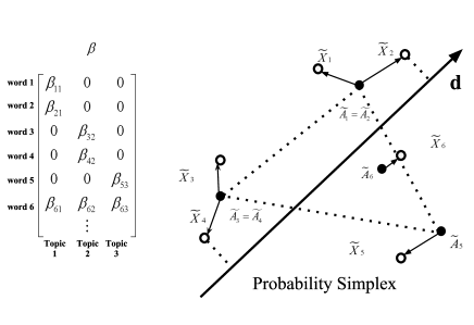
Figure 1: A separable topic matrix and the underlying geometric structure. Solid circles represent rows of $\widetilde{\mathbf{A}}$, empty circles represent rows of $\widetilde{\mathbf{X}}$. Projections of $\widetilde{\mathbf{X}}_{i}$’s along a direction ${\mathbf{d}}$ can be used to identify novel words.

Furthermore, retrieving topic matrix $\bm{\beta}$ is straightforward given all $K$ distinct novel words :

Proposition 2.

If the matrix ${\mathbf{A}}$ and $K$ distinct novel words $\{i_{1},\ldots,i_{K}\}$ are given, then ${\bm{\beta}}$ can be calculated using $W$ linear regressions.

Proof: By Proposition 1, we have $\widetilde{\bm{\theta}}=({\mathbf{A}}_{i_{1}}^{\top},\ldots,{\mathbf{A}}_{i_{K}}^{\top})^{\top}$. Next $\widetilde{\mathbf{A}}_{i}=\widetilde{\bm{\beta}}_{i}\widetilde{\bm{\theta}}$. So $\widetilde{\bm{\beta}}_{i}$ can be computed by solving a linear system of equations. Specifically, if we let ${\bm{\beta}}^{\prime}=\operatorname{diag}(\mathbf{A}\mathbf{1})\widetilde{\bm{\beta}}={\bm{\beta}}\operatorname{diag}(\bm{\theta}\mathbf{1})^{-1}$, ${\bm{\beta}}$ can be obtained by column normalizing ${\bm{\beta}}^{\prime}$.  

Proposition 1 and 2 validate the approach to estimate ${\bm{\beta}}$ via identifying novel words given access to ${\mathbf{A}}$. However, only ${\mathbf{X}}$, a realization of ${\mathbf{A}}$, is available in the real problem which is not close to ${\mathbf{A}}$ in typical settings of interest ($N\ll W$). However, even when the number of samples per document ($N$) is limited, if we collect enough documents ($M\rightarrow\infty$), the proposed algorithm could still asymptotically estimate $\bm{\beta}$ with arbitrary precision, as we will discuss in the following sections.

4 Proposed Algorithm

The geometric intuition mentioned in Propositions 1 and 2 motivates the following three-step approach for topic discovery :

(1) Novel Word Detection: Given the empirical word-by-document matrix $\mathbf{X}$, extract the set of all novel words $\mathcal{I}$. We present variants of projection-based algorithms in Sec. 4.1.

(2) Novel Word Clustering: Given a set of novel words $\mathcal{I}$ with $|\mathcal{I}|\geq K$ , cluster them into $K$ groups corresponding to $K$ topics. Pick a representative for each group. We adopt a distance based clustering algorithm. (Sec. 4.2).

(3) Topic Estimation: Estimate topic matrix as suggested in Proposition 2 by constrained linear regression. (Section 4.3).

4.1 Novel Word Detection

Fig.  1 illustrates the key insight to identify novel words as extreme points of some convex body. When we project every point of a convex body onto some direction $\mathbf{d}$, the maximum and minimum correspond to extreme points of the convex object. Our proposed approaches, data dependent and random projection, both exploit this fact. They only differ in the choice of projected directions.

A. Data Dependent Projections (DDP)
To simplify our analysis, we randomly split each document into two subsets, and obtain two statistically independent document collections $\mathbf{X}$ and $\mathbf{X}^{\prime}$, both distributed as $\mathbf{A}$, and then row normalize as $\widetilde{\mathbf{X}}$ and $\widetilde{\mathbf{X}}^{\prime}$. For some threshold, $d$, to be specified later, and for each word $i$, we consider the set, $J_{i}$, of all other words that are sufficiently different from word $i$ in the following sense:

$$J_{i}=\{j\mid M(\widetilde{\mathbf{X}}_{i}-\widetilde{\mathbf{X}}_{j})(\widetilde{\mathbf{X}}_{i}^{\prime}-\widetilde{\mathbf{X}}_{j}^{\prime})^{\top}\geq d/2\}$$ (1)

We then declare word $i$ as a novel word if all words $j\in J_{i}$ are uniformly uncorrelated to word $i$ with some margin, $\gamma/2$ to be specified later.

$$M\langle\widetilde{\mathbf{X}}_{i},\widetilde{\mathbf{X}}_{i}^{\prime}\rangle\geq M\langle\widetilde{\mathbf{X}}_{i},\widetilde{\mathbf{X}}_{j}^{\prime}\rangle+\gamma/2,\,\,\forall j\in J_{i}$$ (2)

The correctness of DDP Algorithm is established by the following Proposition and will be further discussed in section 5. The proof is given in the Supplementary section.

Proposition 3.

Suppose conditions $P1$ and $P2$ (will be defined in section 5) on prior distribution of ${\bm{\theta}}$ hold. Then, there exists two positive constants $d$ and $\gamma$ such that if $i$ is a novel word, for all $j\in J_{i}$, $M\langle\widetilde{\mathbf{X}}_{i},\widetilde{\mathbf{X}}_{i}^{\prime}\rangle-M\langle\widetilde{\mathbf{X}}_{i},\widetilde{\mathbf{X}}_{j}^{\prime}\rangle\geq\gamma/2$ with high probability (converging to one as $M\rightarrow\infty$). In addition, if $i$ is a non-novel word, there exists some $j\in J_{i}$ such that $M\langle\widetilde{\mathbf{X}}_{i},\widetilde{\mathbf{X}}_{i}^{\prime}\rangle-M\langle\widetilde{\mathbf{X}}_{i},\widetilde{\mathbf{X}}_{j}^{\prime}\rangle\leq\gamma/2$ with high probability.

Algorithm 1 Novel Word Detection - DDP

1:  Input $\widetilde{\mathbf{X}},\widetilde{\mathbf{X}}^{\prime},d,\gamma,K$

2:  Output: The indices of the novel words $\mathcal{I}$

3:  ${\mathbf{C}}\leftarrow M~{}\widetilde{\mathbf{X}}^{\prime}\widetilde{\mathbf{X}}^{\top}$

4:  $\mathcal{I}\leftarrow\emptyset$

5:  for all $1\leq i\leq W$ do

6:     $J_{i}\leftarrow$ All indices $j\neq i:C_{i,i}-2C_{i,j}+C_{j,j}\geq\frac{d}{2}$

7:     if $\forall j\in J_{i}~{}:~{}C_{i,i}-C_{i,j}\geq\gamma/2$ then

8:        $\mathcal{I}\leftarrow\mathcal{I}\cup\{i\}$

9:     end if

10:  end for

The algorithm is elaborated in Algorithm 1. The running time of the algorithm is summarized in the following proposition. Detailed justification is provided in the Supplementary section.

Proposition 4.

The running time of Algorithm 1 is $\mathcal{O}(MN^{2}+W^{2})$.

Proof Sketch. Note that ${\mathbf{X}}$ is sparse since $N\ll W$. Hence by exploiting the sparsity ${\mathbf{C}}=M{\mathbf{X}}{\mathbf{X}}^{\prime\top}$ can be computed in $\mathcal{O}(MN^{2}+W)$ time. For each word $i$, finding $J_{i}$ and calculating $C_{i,i}-C_{i,j}\geq\gamma/2$ cost $\mathcal{O}(W^{2})$ time in the worst case.  

B. Random Projections (RP)
DDP uses $W$ different directions to find all the extreme points. Here we use random directions instead. This significantly reduces the time complexity by decreasing the number of required projections.

The Random Projection Algorithm (RP) uses roughly $P=\mathcal{O}(K)$ random directions drawn uniformly iid over the unit sphere. For each direction ${\mathbf{d}}$, we project all $\widetilde{\mathbf{X}}_{i}$’s onto it and choose the maximum and minimum.

Algorithm 2 Novel Word Detection - RP

1:  Input $\widetilde{\mathbf{X}},P$

2:  Output : The indices of the novel words $\mathcal{I}$

3:  $\mathcal{I}\leftarrow\emptyset$

4:  for all $1\leq j\leq P$ do

5:     Generate ${\mathbf{d}}\sim$ Uniform(unit-sphere in ${\mathbb{R}}^{M}$)

6:     $i_{max}=\operatorname*{arg\,max}\widetilde{\mathbf{X}}_{i}{\mathbf{d}},i_{min}=\operatorname*{arg\,max}\widetilde{\mathbf{X}}_{i}{\mathbf{d}}$

7:     $\mathcal{I}\leftarrow\mathcal{I}\cup\{i_{max},i_{min}\}$

8:  end for

Note that $\widetilde{\mathbf{X}}_{i}{\mathbf{d}}$ will converge to $\widetilde{\mathbf{A}}_{i}{\mathbf{d}}$ conditioned on ${\mathbf{d}}$ and ${\bm{\theta}}$ as $M$ increases. Moreover, only for the extreme points $i$, $\widetilde{\mathbf{A}}_{i}{\mathbf{d}}$ can be the maximum or minimum projection value. This provides intuition of consistency for RP. Since the directions are independent, we expect to find all the novel words using $P=\mathcal{O}(K)$ number of random projections.

C. Random Projections with Binning

Another alternative to RP is a Binning algorithm which is computationally more efficient. Here the corpus is split into $\sqrt{M}$ equal sized bins. For each bin $j$ a random direction ${\mathbf{d}}^{(j)}$ is chosen and the word with the maximum projection along ${\mathbf{d}}^{(j)}$ is chosen as a winner. Then, we find the number of wins for each word $i$. We then divide these winning frequencies by $\sqrt{M}$ as an estimate for $p_{i}\triangleq\Pr(\forall j\neq i:\widetilde{\mathbf{A}}_{i}{\mathbf{d}}\geq\widetilde{\mathbf{A}}_{j}{\mathbf{d}})$. $p_{i}$ can be shown to be zero for all non-novel words. For non-degenerate prior over ${\bm{\theta}}$, these probabilities converge to strictly positive values for novel words. Hence, estimating $p_{i}$’s helps in identifying novel words. We then choose the indices of $\mathcal{O}(K)$ largest $p_{i}$ values as novel words. The Binning algorithm is outlined in Algorithm 3.

Algorithm 3 Novel Word Detection - Binning

1:  Input : $\widetilde{\mathbf{X}}$, $\widetilde{\mathbf{X}}^{\prime}$, $d$, K

2:  Output : The indices of the novel words $\mathcal{I}$

3:  Split documents in ${\mathbf{X}}$ into $\sqrt{M}$ equal sized groups of documents ${\mathbf{X}}^{(1)},\ldots,{\mathbf{X}}^{(\sqrt{M})}$ and normalize each one separately to obtain $\widetilde{\mathbf{X}}^{(1)},\ldots,\widetilde{\mathbf{X}}^{(\sqrt{M})}$ as well.

4:  for all $1\leq j\leq\sqrt{M}$ do

5:     ${\mathbf{d}}^{(j)}\leftarrow$ a sample from $U(\mathcal{S}^{\sqrt{M}-1})$

6:     $l\leftarrow\operatorname*{arg\,max}\limits_{1\leq i\leq W}\widetilde{\mathbf{X}}^{(j)}_{i}{\mathbf{d}}^{(j)}$

7:     $\hat{p}_{l}^{(j)}\leftarrow\hat{p}_{l}^{(j)}+1$

8:  end for

9:  for all $1\leq i\leq W$ do

10:     $\hat{p}_{i}\leftarrow\frac{1}{\sqrt{M}}\sum_{j=1}^{\sqrt{M}}\hat{p}_{i}^{(j)}$

11:  end for

12:  $k\leftarrow 0$, $\mathcal{I}\leftarrow\emptyset$ and $i\leftarrow 1$

13:  repeat

14:     $j\leftarrow$ the index of the $i^{\text{th}}$ largest value of $(\hat{p}_{1},\ldots,\hat{p}_{W})$

15:     if ${\mathcal{I}}=\emptyset\text{ or }\forall l\in\mathcal{I}:M(\widetilde{\mathbf{X}}_{j}-\widetilde{\mathbf{X}}_{l})(\widetilde{\mathbf{X}}_{j}^{\prime}-\widetilde{\mathbf{X}}_{l}^{\prime})\geq d/2$  then

16:        $\mathcal{I}\leftarrow\mathcal{I}\cup\{j\}$

17:        $k\leftarrow k+1$

18:     end if

19:     $i\leftarrow i+1$

20:  until $k=K$

In contrast with DDP, the RP algorithm is completely agnostic and parameter-free. This means that it requires no parameters like $d$ and $\gamma$ to find the novel words. Moreover, it significantly reduces the computational complexity :

Proposition 5.

The running times of the RP and Binning algorithms are $\mathcal{O}(MNK+WK)$ and $\mathcal{O}(MN+\sqrt{M}W)$, respectively.

Proof.

We will sketch the proof and provide a more detailed justification in the Supplementary section. Note that the number of operations needed to find the projections is $\mathcal{O}(MN+W)$ in Binning and $\mathcal{O}(MNK+W)$ in RP. In addition, finding the the maximum takes $\mathcal{O}(WK)$ for RP and $\mathcal{O}(\sqrt{M}W)$ for Binning. In sum, it takes $\mathcal{O}(MNK+WK)$ for RP and $\mathcal{O}(MN+\sqrt{M}W)$ for Binning to find all the novel words. ∎

4.2 Novel Word Clustering

Since there may be multiple novel words for a single topic, our DDP or RP algorithm can extract multiple novel words for each topic. This necessitates clustering to group the copies. We can show that our clustering scheme is consistent if we assume that ${\mathbf{R}}=\frac{1}{M}\operatorname{\mathbb{E}}({\bm{\theta}}{\bm{\theta}}^{\top})$ is positive definite:

Proposition 6.

Let $C_{i,j}\triangleq M\widetilde{\mathbf{X}}_{i}\widetilde{\mathbf{X}}_{j}^{\prime\top}$, and $D_{i,j}\triangleq C_{i,i}-2C_{i,j}+C_{j,j}$. If ${\mathbf{R}}$ is positive definite, then $D_{i,j}$ converges to zero in probability whenever $i$ and $j$ are novel words of the same topic as $M\rightarrow\infty$. Moreover, if $i$ and $j$ are novel words of different types, it converges in probability to some strictly positive value greater than some constant $d$ .

The proof is presented in the Supplementary section.

Algorithm 4 Novel Word Clustering

1:  Input : $\mathcal{I}$, $\widetilde{\mathbf{X}}$, $\widetilde{\mathbf{X}}^{\prime}$, $d$, $K$

2:  Output : $\mathcal{J}$ which is a set of $K$ novel words of distinct topics

3:  ${\mathbf{C}}\leftarrow M~{}\widetilde{\mathbf{X}}^{\prime}\widetilde{\mathbf{X}}^{\top}$

4:  ${\mathbf{B}}\leftarrow\text{a }|\mathcal{I}|\times|\mathcal{I}|\text{ zero matrix}$

5:  for all $i,j\in\mathcal{I},~{}i\neq j$ do

6:     if $C_{i,i}-2C_{i,j}+C_{j,j}\leq d/2$ then

7:        $B_{i,j}\leftarrow 1$

8:     end if

9:  end for

10:  $\mathcal{J}\leftarrow\emptyset$

11:  for all $1\leq j\leq K$ do

12:     $c\leftarrow$ one of the indices of the $j^{\text{th}}$ connected component vertices in ${\mathbf{B}}$

13:     $\mathcal{J}\leftarrow\mathcal{J}\cup\{c\}$

14:  end for

As the Proposition 6 suggests, we construct a binary graph with its vertices correspond to the novel words. An edge between word $i$ and $j$ is established if $D_{i,j}\leq d/2$. Then, the clustering reduces to finding $K$ connected components. The procedure is described in Algorithm 4.

In Algorithm 4, we simply choose any word of a cluster as the representative for each topic. This is simply for theoretical analysis. However, we could set the representative to be the average of data points in each cluster, which is more noise resilient.

4.3 Topic Matrix Estimation

Given $K$ novel words of different topics ($\mathcal{J}$), we could directly estimate (${\bm{\beta}}$) as in Proposition 2. This is described in Algorithm 5. We note that this part of the algorithm is similar to some other topic modeling approaches, which exploit separability. Consistency of this step is also validated in (Arora et al., 2012b). In fact, one may use the convergence of extremum estimators (Amemiya, 1985) to show the consistency of this step.

Algorithm 5 Topic Matrix Estimation

1:  Input: $\mathcal{J}=\{j_{1},\ldots,j_{K}\}$, ${\mathbf{X}}$, ${\mathbf{X}}^{\prime}$

2:  Output: $\widehat{{\bm{\beta}}}$, which is the estimation of ${\bm{\beta}}$ matrix

3:  ${\mathbf{Y}}=(\widetilde{\mathbf{X}}_{j_{1}}^{\top},\ldots,\widetilde{\mathbf{X}}_{j_{K}}^{\top})^{\top}$,${\mathbf{Y}^{\prime}}=(\widetilde{\mathbf{X}}_{j_{1}}^{{\prime}\top},\ldots,\widetilde{\mathbf{X}}_{j_{K}}^{{\prime}\top})^{\top}$

4:  for all $1\leq i\leq W$ do

5:     $\widehat{\bm{\beta}}_{i}\leftarrow(\frac{1}{M}{\mathbf{X}}_{i}{\mathbf{1}})\operatorname*{arg\,min}\limits_{b_{j}\geq 0,\sum_{j=1}^{K}b_{j}=1}M(\widetilde{\mathbf{X}}_{i}-{\mathbf{b}}{\mathbf{Y}})(\widetilde{\mathbf{X}}^{\prime}_{i}-{\mathbf{b}}{\mathbf{Y}}^{\prime})^{\top}$

6:  end for

7:  column normalize $\widehat{\bm{\beta}}$

5 Statistical Complexity Analysis

In this section, we describe the sample complexity bound for each step of our algorithm. Specifically, we provide guarantees for DDP algorithm under some mild assumptions on the distribution over ${\bm{\theta}}$. The analysis of the random projection algorithm is much more involved and requires elaborate arguments. We will omit it in this paper.

We require following technical assumptions on the correlation matrix ${\mathbf{R}}$ and the mean vector ${\mathbf{a}}$ of ${\bm{\theta}}$ :

$({P1})$ ${\mathbf{R}}$ is positive definite with its minimum eigenvalue being lower bounded by $\lambda_{\wedge}>0$. In addition, $\forall i,{a}_{i}\geq a_{\wedge}>0$.

$({P2})$ There exists a positive value $\zeta$ such that for $i\neq j$, $R_{i,i}/(a_{i}a_{i})-R_{i,j}/(a_{i}a_{j})\geq\zeta$.

The second condition captures the following intuition : if two novel words are from different topics, they must appear in a substantial number of distinct documents. Note that for two novel words $i$ and $j$ of different topics, $M\widetilde{\mathbf{A}}_{i}(\widetilde{\mathbf{A}}_{i}-\widetilde{\mathbf{A}}_{j})^{\top}\xrightarrow{p}R_{i,i}/(a_{i}a_{i})-R_{i,j}/(a_{i}a_{j})$. Hence, this requirement means that $M(\widetilde{\mathbf{A}}_{i}-\widetilde{\mathbf{A}}_{j})$ should be fairly distant from the origin, which implies that the number of documents these two words co-occur in, with similar probabilities, should be small. This is a reasonable assumption, since otherwise we would rather group two related topics into one. In fact, we show in the Supplementary section (Section A.5) that both conditions hold for the Dirichlet distribution, which is a traditional choice for the prior distribution in topic modeling. Moreover, we have tested the validity of these assumptions numerically for the logistic normal distribution (with non-degenerate covariance matrices), which is used in Correlated Topic Modeling (CTM) (Blei & Lafferty, 2007).

5.1 Novel Word Detection Consistency

In this section, we provide analysis only for the DDP Algorithm. The sample complexity analysis of the randomized projection algorithms is however more involved and is the subject of the ongoing research. Suppose $P1$ and $P2$ hold. Denote $\beta_{\wedge}$ and $\lambda_{\wedge}$ to be positive lower bounds on non-zero elements of ${\bm{\beta}}$ and minimum eigenvalue of ${\mathbf{R}}$, respectively. We have:

Theorem 1.

For parameter choices $d={\lambda_{\wedge}\beta_{\wedge}^{2}}$ and $\gamma=\zeta{a_{\wedge}\beta_{\wedge}}$ the DDP algorithm is consistent as $M\rightarrow\infty$. Specifically, true novel and non-novel words are asymptotically declared as novel and non-novel, respectively. Furthermore, for

$$M\geq\frac{C_{1}\left(\log W+\log\left(\frac{1}{\delta_{1}}\right)\right)}{\beta_{\wedge}^{2}\eta^{8}\min(\lambda_{\wedge}^{2}\beta_{\wedge}^{2},\zeta^{2}a_{\wedge}^{2})}$$

where $C_{1}$ is a constant, Algorithm 1 finds all novel words without any outlier with probability at least $1-\delta_{1}$, where $\eta=\min\limits_{1\leq i\leq W}{\bm{\beta}}_{i}{\mathbf{a}}$.

Proof Sketch. The detailed justification is provided in the Supplementary section. The main idea of the proof is a sequence of statements :

• Given $P1$, for a novel word $i$, $J_{i}$ defined in the Algorithm 1 is a subset of $J_{i}^{*}$ asymptotically with high probability, where $J_{i}^{*}=\{j:\operatorname{supp}({\bm{\beta}}_{j})\neq\operatorname{supp}({\bm{\beta}}_{i})\}$. Moreover $J_{i}$ is a superset of $J^{*}_{i}$ with high probability for a non-novel word with $J_{i}^{*}=\{j:|\operatorname{supp}({\bm{\beta}}_{j})|=1\}$.

• Given $P2$, for a novel word $i$, $C_{i,i}-C_{i,j}$ converges to a strictly positive value greater than $\gamma$ for $j\in J_{i}^{*}$, and if $i$ is non-novel, $\exists j\in J_{i}^{*}$ such that $C_{i,i}-C_{i,j}$ converges to a non-positive value.

These statements imply Proposition 3, which proves the consistency of the DDP Algorithm.  

The term $\eta^{-8}$ seems to be the dominating factor in the sample complexity bound. Basically, $\eta=\min\limits_{1\leq i\leq W}\frac{1}{M}\operatorname{\mathbb{E}}({\mathbf{X}}_{i}{\mathbf{1}})$ represents the minimum proportion of documents that a word would appear in. This is not surprising as the rate of convergence of $C_{i,j}=M\langle\widetilde{\mathbf{X}}_{i},\widetilde{\mathbf{X}}_{j}^{\prime}\rangle$ is dependent on the values of $\frac{1}{M}\operatorname{\mathbb{E}}({\mathbf{X}}_{i}{\mathbf{1}})$ and $\frac{1}{M}\operatorname{\mathbb{E}}({\mathbf{X}}_{j}{\mathbf{1}})$. As these values are decreased, $C_{i,j}$ converges to a larger value and the convergence get slower. In another view, given that the number of words per document $N$ is bounded, in order to have $C_{i,j}$ converge, a large number of documents is needed to observe all the words sufficiently. It is remarkable that a similar term $p^{-6}$ would also arise in the sample complexity bound of (Arora et al., 2012b), where $p$ is the minimum non-zero element of diagonal part of ${\bm{\beta}}$. It may be noted that although it seems that the sample complexity bound scales logarithmically with $W$, $\eta$ and $p$ would be decreased typically as $W$ increases.

5.2 Novel Word Clustering Consistency

We similarly prove the consistency and sample complexity of the novel word clustering algorithm :

Theorem 2.

For $d={\lambda_{\wedge}\beta_{\wedge}^{2}}$, given all true novel words as the input, the clustering algorithm, Algorithm 4 (ClusterNovelWords) asymptotically (as $M\rightarrow\infty$ recovers $K$ novel word indices of different types, namely, the support of the corresponding ${\bm{\beta}}$ rows are different for any two retrieved indices. Furthermore, if

$$M\geq\frac{C_{2}\left(\log W+\log\left(\frac{1}{\delta_{2}}\right)\right)}{\eta^{8}\lambda_{\wedge}^{2}\beta_{\wedge}^{4}}$$

then Algorithm 4 clusters all novel words correctly with probability at least $1-\delta_{2}$.

Proof Sketch. More detailed analysis is provided in the Supplementary section. We can show that $C_{i,i}-2C_{i,j}+C_{j,j}$ converges to a strictly positive value $d$ if $i$ and $j$ are novel words of different topics. Moreover, it converges to zero if they are novel words of the same topic. Hence all novel words of the same topic are connected in the graph with high probability asymptotically. Moreover, there would not be an edge between the novel words of different topics with high probability. Therefore, the connected components of the graph corresponds to the true clusters asymptotically. The detailed discussion of the convergence rate is provided in the Supplementary section.  

It is noticeable that the sample complexity of the clustering is similar to that of the novel word detection. This means that the hardness of novel word detection and distance based clustering using the proposed algorithms are almost the same.

5.3 Topic Estimation Consistency

Finally, we show that the topic estimation by regression is also consistent.

Theorem 3.

Suppose that Algorithm 5 outputs $\widehat{\bm{\beta}}$ given the indices of $K$ distinct novel words. Then, $\widehat{\bm{\beta}}\xrightarrow{p}{\bm{\beta}}$. Specifically, if

$$M\geq\frac{C_{3}W^{4}(\log(W)+\log(K)+\log(1/\delta_{3}))}{\lambda_{\wedge}^{2}\eta^{8}\epsilon^{4}a_{\wedge}^{8}}$$

then for all $i$ and $j$, $\widehat{\beta}_{i,j}$ will be $\epsilon$ close to $\beta_{i,j}$ with probability at least $1-\delta_{3}$, with $\epsilon<1$, $C_{3}$ being a constant, $a_{\wedge}=\min_{i}a_{i}$ and $\eta=\min\limits_{1\leq i\leq W}{\bm{\beta}}_{i}{\mathbf{a}}$.

Proof Sketch. We will provide a detailed analysis in the Supplementary section. To prove the consistency of the regression algorithm, we will use a consistency result for the extremum estimators : If we assume $Q_{M}({\bm{\beta}})$ to be a stochastic objective function which is minimized at $\widehat{\bm{\beta}}$ under the constraint ${\bm{\beta}}\in\Theta$ (for a compact $\Theta$), and ${Q}_{M}({\bm{\beta}})$ converges uniformly to $\bar{Q}({\bm{\beta}})$, which in turn is minimized uniquely in ${\bm{\beta}}^{*}$, then $\widehat{\bm{\beta}}\xrightarrow{p}{\bm{\beta}}^{*}$ (Amemiya, 1985). In our setting, we may take $Q_{M}$ to be the objective function in Algorithm 5. Then, $Q_{M}({\mathbf{b}})\xrightarrow{p}\bar{Q}({\mathbf{b}})={\mathbf{b}}{\mathbf{D}}{\mathbf{R}}{\mathbf{D}}{\mathbf{b}}^{\top}-2{\mathbf{b}}{\mathbf{D}}{\mathbf{R}}\frac{{\bm{\beta}}_{i}^{\top}}{{\bm{\beta}}_{i}{\mathbf{a}}}+\frac{{\bm{\beta}}_{i}}{{\bm{\beta}}_{i}{\mathbf{a}}}{\mathbf{R}}\frac{{\bm{\beta}}_{i}^{\top}}{{\bm{\beta}}_{i}{\mathbf{a}}}$, where ${\mathbf{D}}=\operatorname{diag}({\mathbf{a}})^{-1}$. Note that if ${\mathbf{R}}$ is positive definite, $\bar{Q}$ is uniquely minimized at ${\mathbf{b}}^{*}=\frac{{\bm{\beta}}_{i}}{{\bm{\beta}}_{i}{\mathbf{a}}}{\mathbf{D}}^{-1}$, which satisfies the conditions of the optimization. Moreover, ${Q}_{M}$ converges to $Q$ uniformly as a result of Lipschitz continuity of $Q_{M}$. Therefore, according to Slutsky’s theorem, $(\frac{1}{M}{\mathbf{X}}_{i}{\mathbf{1}}){\mathbf{b}}^{*}=\widehat{\bm{\beta}}_{i}$ converges to ${\bm{\beta}}_{i}{\mathbf{D}}^{-1}$, and hence the column normalization of $\widehat{\bm{\beta}}$ converges to ${\bm{\beta}}$. We will provide a more detailed analysis of this part in the Supplementary section.  

In sum, consider the approach outlined at the beginning of section 4 based on data-dependent projections method, and assume that $\widehat{\bm{\beta}}$ is the output. Then,

Theorem 4.

The output of the topic modeling algorithm $\widehat{\bm{\beta}}$ converges in probability to ${\bm{\beta}}$ element-wise. To be precise, if

$$M\geq\max\left\{\frac{C_{2}^{\prime}W^{4}\log\frac{WK}{\delta}}{\lambda_{\wedge}^{2}\eta^{8}\epsilon^{4}a_{\wedge}^{8}},\frac{C_{1}^{\prime}\log\frac{W}{\delta}}{\beta_{\wedge}^{2}\eta^{8}\min(\lambda_{\wedge}^{2}\beta_{\wedge}^{2},\zeta^{2}a_{\wedge}^{2})}\right\}$$

then with probability at least $1-3\delta$, for all $i$ and $k$, $\widehat{\beta}_{i,k}$ will be $\epsilon$ close to $\beta_{i,k}$, with $\epsilon<1$, $C_{1}^{\prime}$ and $C_{2}^{\prime}$ being two constants.

The proof is a combination of Theorems 1, 2 and 3.

6 Experimental Results

6.1 Practical Considerations

DDP algorithm requires two parameters $\gamma$ and $d$. In practice, we can apply DDP without knowing them adaptively and agnostically. Note that $d$ is for the construction of $J_{i}$. We can otherwise construct $J_{i}$ by finding $r<W$ words that are maximally distant from $i$ in the sense of Eq. 1. To bypass $\gamma$, we can rank the values of $\min_{j\in J_{i}}M\langle\widetilde{\mathbf{X}}_{i},\widetilde{\mathbf{X}}_{i}^{\prime}\rangle-M\langle\widetilde{\mathbf{X}}_{i},\widetilde{\mathbf{X}}_{j}^{\prime}\rangle$ across all $i$ and declare the topmost $s$ values as the novel words.

The clustering algorithm also requires parameter $d$. Note that $d$ is just for thresholding a $0-1$ weighted graph. In practice, we could avoid hard thresholding by using $\exp(-(C_{i,i}-2C_{i,j}+C_{j,j}))$ as weights for the graph and apply spectral clustering. To point out, typically the size of $\mathcal{I}$ in Algorithm 4 is of the same order as $K$. Hence the spectral clustering is on a relative small graph which typically adds $\mathcal{O}(K^{3})$ computational complexity.

Implementation Details: We choose the parameters of the DDP and RP in the following way. For DDP in all datasets except the Donoho image corpus, we use the agnostic algorithm discussed in section 6.1 with $r=W/2$. Moreover, we take $s=10\times K$. For the image dataset, we used $d=1$ and $\gamma=3$. For RP, we set the number of projections $P\approx 50\times K$ in all datasets to obtain the results.

6.2 Synthetic Dataset

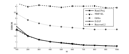
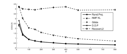
Figure 2: Error of estimated topic matrix in $\ell_{1}$ norm. Upper: $W=500,\rho=0.2,N=100,K=5$; Lower: $W=500,\rho=0.2,M=500,K=10$. Top and Bottom plots depict error with varying documents $M$ (for fixed $N$) and varying words $N$ (for fixed $M$) respectively. RP & DDP show consistently better performance.

In this section, we validate our algorithm on synthetic examples. We generate a $W\times K$ separable topic matrix ${\bm{\beta}}$ with $W_{1}/K>1$ novel words per topic as follows: first, iid $1\times K$ row-vectors corresponding to non-novel words are generated uniformly on the probability simplex. Then, $W_{1}$ iid $\mathrm{Uniform}[0,1]$ values are generated for the nonzero entries in the rows of novel words. The resulting matrix is then column-normalized to get one realization of ${\bm{\beta}}$. Let $\rho:=W_{1}/W$. Next, $M$ iid $K\times 1$ column-vectors are generated for the $\theta$ matrix according to a Dirichlet prior $c\prod\limits_{i=1}^{K}\theta_{i}^{\alpha_{i}-1}$. Following (Griffiths & Steyvers, 2004), we set $\alpha_{i}=0.1$ for all $i$. Finally, we obtain ${\mathbf{X}}$ by generating $N$ iid words for each document.

For different settings of $W$, $\rho$, $K$, $M$ and $N$, we calculate the $\ell_{1}$ distance of the estimated topic matrix to the ground truth after finding the best matching between two sets of topics. For each setting we average the error over $50$ random samples. For RP & DDP we set parameters as discussed in the implementation details.

We compare the DDP and RP against the Gibbs sampling approach (Griffiths & Steyvers, 2004) (Gibbs), a state-of-art NMF-based algorithm (Tan & Févotte, in press) (NMF) and the most recent practical provable algorithm in (Arora et al., 2012a) (RecL2). The NMF algorithm is chosen because it compensates for the type of noise in our topic model. Fig.  2 depicts the estimation error as a function of the number of documents $M$ (Upper) and the number of words/document $N$ (bottom). RP and DDP have similar performance and are uniformly better than comparable techniques. Gibbs performs relatively poor in the first setting and NMF in the second. RecL2 perform worse in all the settings. Note that $M$ is relatively small ($\leq 1,000$) compared to $W=500$. DDP/RP outperform other methods with fairly small sample size. Meanwhile, as is also observed in (Arora et al., 2012a), RecL2 has a poor performance with small $M$.

6.3 Swimmer Image Dataset

(a)		(b)		(c)

Figure 3: (a) Example “clean” images in Swimmer dataset; (b) Corresponding images with sampling “noise” ; (c) Examples of ideal topics.

a)
b)
c)
d)

Figure 4: Topic errors for (a) Gibbs (Griffiths & Steyvers, 2004), (b) NMF (Tan & Févotte, in press) and c) example Topics extracted by RecL2 (Arora et al., 2012a) on the noisy Swimmer dataset. d) Example Topic errors for RecL2 on clean Swimmer dataset. Figure depicts extracted topics that are not close to any “ground truth”. The ground truth topics correspond to 16 different positions of left/right arms and legs.

Pos.	LA 1	LA 2	LA 3	LA 4	RA 1	RA 2	RA 3	RA 4	LL 1	LL 2	LL 3	LL 4	RL 1	RL 2	RL 3	RL 4
a)
b)
c)
d)
e)

Figure 5: Topics estimated for noisy swimmer dataset by a) proposed RP, b) proposed DDP, c) Gibbs in (Griffiths & Steyvers, 2004), d) NMF in (Tan & Févotte, in press) and e) on clean dataset by RecL2 in (Arora et al., 2012a) closest to the 16 ideal (ground truth) topics. Gibbs misses $5$ and NMF misses $6$ of the ground truth topics while RP DDP recovers all $16$ and our topic estimates look less noisy. RecL2 hits $4$ on clean dataset.

In this section we apply our algorithm to the synthetic swimmer image dataset introduced in (Donoho & Stodden, 2004). There are $M=256$ binary images, each with $W=32\times 32=1024$ pixels. Each image represents a swimmer composed of four limbs, each of which can be in one of $4$ distinct positions, and a torso. We interpret pixel positions $(i,j)$ as words. Each image is interpreted as a document composed of pixel positions with non-zero values. Since each position of a limb features some unique pixels in the image, the topic matrix $\bm{\beta}$ satisfies the separability assumption with $K=16$ “ground truth” topics that correspond to $16$ single limb positions.

Following the setting of (Tan & Févotte, in press), we set body pixel values to 10 and background pixel values to 1. We then take each “clean” image, suitably normalized, as an underlying distribution across pixels and generate a “noisy” document of $N=200$ iid “words” according to the topic model. Examples are shown in Fig. 3. We then apply RP and DDP algorithms to the “noisy” dataset and compare against Gibbs (Griffiths & Steyvers, 2004), NMF (Tan & Févotte, in press), and RecL2 (Arora et al., 2012a). Results are shown in Figs. 4 and 5. We set the parameters as discussed in the implementation details.

This dataset is a good validation test for different algorithms since the ground truth topics are known and unique. As we see in Fig. 4, both Gibbs and NMF produce topics that do not correspond to any pure left/right arm/leg positions. Indeed, many of them are composed of multiple limbs. Nevertheless, as shown in Fig. 5, no such errors are realized in RP and DDP and our topic-estimates are closer to the ground truth images. In the meantime, RecL2 algorithm failed to work even with the clean data. Although it also extracts extreme points of a convex body, the algorithm additionally requires these points to be linearly independent. It is possible that extreme points of a convex body are linearly dependent (for example, a 2-D square on a 3-D simplex). This is exactly the case in the swimmer dataset. As we see in the last row in Fig. 5, RecL2 produces only a few topics close to ground truth. Its extracted topics for the noisy images are shown in Fig. 4. Results of RecL2 on noisy images are no close to ground truth as shown in Fig. 4.

6.4 Real World Text Corpora

Table 1: Examples of extracted topics for NIPS dataset by proposed Random projection method (RP), Data-dependent projection (DDP), algorithm in (Griffiths & Steyvers, 2004)(Gibbs), the practical algorithm in (Arora et al., 2012a)(RecL2).

RP	chip circuit noise analog current voltage gates
DDP	chip circuit analog voltage pulse vlsi device
Gibbs	analog circuit chip output figure current vlsi
RecL2	N/A
RP	visual cells spatial ocular cortical cortex dominance orientation
DDP	visual cells model cortex orientation cortical eye
Gibbs	cells cortex visual activity orientation cortical receptive
RecL2	orientation knowledge model cells visual good mit
RP	learning training error vector parameters svm data
DDP	learning error training weight network function neural
Gibbs	training error set generalization examples test learning
RecL2	training error set data function test weighted
RP	speech training recognition performance hmm mlp input
DDP	training speech recognition network word classifiers hmm
Gibbs	speech recognition word training hmm speaker mlp acoustic
RecL2	speech recognition network neural positions training learned

Table 2: Examples of estimated topics on NY Times using RP and RecL2 algorithms

RP	weather wind air storm rain cold
RecL2	N/A
RP	feeling sense love character heart emotion
RecL2	N/A
RP	election zzz_florida ballot vote zzz_al_gore recount
RecL2	ballot election court votes vote zzz_al_gore
RP	yard game team season play zzz_nfl
RecL2	yard game play season team touchdown
RP	N/A
RecL2	zzz_kobe_bryant zzz_super_bowl police shot family election

In this section, we apply our algorithm on two different real world text corpora from (Frank & Asuncion, 2010). The smaller corpus is NIPS proceedings dataset with $M=1,700$ documents, a vocabulary of $W=14,036$ words and an average of $N\approx 900$ words in each document. Another is a large corpus New York (NY) Times articles dataset, with $M=300,000$, $W=102,660$, and $N\approx 300$. The vocabulary is obtained by deleting a standard “stop” word list used in computational linguistics, including numbers, individual characters, and some common English words such as “the”.

In order to compare with the practical algorithm in (Arora et al., 2012a), we followed the same pruning in their experiment setting to shrink the vocabulary size to $W=2,500$ for NIPS and $W=15,000$ for NY Times. Following typical settings in (Blei, 2012) and (Arora et al., 2012a), we set $K=40$ for NIPS and $K=100$ for NY Times. We set our parameters as discussed in implementation details.

We compare DDP and RP algorithms against RecL2 (Arora et al., 2012a) and a practically widely successful algorithm (Griffiths & Steyvers, 2004)(Gibbs). Table 1 and 2 depicts typical topics extracted by the different methods. For each topic, we show its most frequent words, listed in descending order of the estimated probabilities. Two topics extracted by different algorithms are grouped if they are close in $\ell_{1}$ distance.

Different algorithms extract some fraction of similar topics which are easy to recognize. Table 1 indicates most of the topics extracted by RP and DDP are similar and are comparable with that of Gibbs. We observe that the recognizable themes formed with DDP or RP topics are more abundant than that by RecL2. For example, topic on “chip design” as shown in the first panel in Table 1 is not extracted by RecL2, and topics in Table 2 on “weather” and “emotions” are missing in RecL2. Meanwhile, RecL2 method produces some obscure topics. For example, in the last panel of Table 1, RecL2 contains more than one theme, and in the last panel of Table 2 RecL2 produce some unfathomable combination of words. More details about the topics extracted are given in the Supplementary section.

Table 3: Comparison of Approaches. Recover from (Arora et al., 2012b); RecL2 from (Arora et al., 2012a); ECA from (Anandkumar et al., 2012); Gibbs from (Griffiths & Steyvers, 2004); NMF from (Lee & Seung, 1999). $Time_{W}(L.P)$, $Time_{K}(L.R)$ stands for computation time for Linear Programming or Linear Regression for $W$ and $K$ number of variables respectively; The definition of the set of parameters can be found in the reference papers.

Method	Computational Complexity	Sample complexity($M$)	Assumptions	Remarks
DDP	$\mathcal{O}(N^{2}M+W^{2})+W~{}Time_{K}(L.R)$	$$\max\Big{\{}\frac{C_{2}^{\prime}W^{4}\log\frac{WK}{\delta}}{\lambda_{\wedge}^{2}\eta^{8}\epsilon^{4}a_{\wedge}^{8}},\\ \frac{C_{1}^{\prime}\log\frac{W}{\delta}}{\beta_{\wedge}^{2}\eta^{8}\min(\lambda_{\wedge}^{2}\beta_{\wedge}^{2},\zeta^{2}a_{\wedge}^{2})}\Big{\}}$$	Separable $\bm{\beta}$; $P1$ and $P2$ on Prior Distribution of ${\bm{\theta}}$ (Sec. 5); Knowledge of $\gamma$ and $d$ (defined in Algorithm 1)	$\Pr({\text{Error}})\rightarrow 0$ exponentially
RP	$\mathcal{O}(MNK+WK)+W~{}Time_{K}(L.R)$	N/A	Separable $\bm{\beta}$
Binning	$\mathcal{O}(MN+\sqrt{M}W)+W~{}Time_{K}(L.R)$	N/A	Separable $\bm{\beta}$
Recover (Arora et al., 2012b)	$\mathcal{O}(MN^{2})+$ $W~{}Time_{W}(L.P)+W~{}Time_{K}(L.R)$	$\max\left\{\frac{C\log(W)a^{4}K^{6}}{\epsilon^{2}p^{6}\gamma^{2}},\frac{a^{2}K^{4}\log K}{\gamma^{2}}\right\}$	Separable $\bm{\beta}$; Robust Simplicial Property of ${\mathbf{R}}$	$\Pr({\text{Error}})\rightarrow 0$; Too many Linear Programmings make the algorithm impractical
RecL2 (Arora et al., 2012a)	$\mathcal{O}(W^{2}+WK/\epsilon^{2}+$ $MN^{2})+$ $W~{}Time_{K}(L.R)$	$\max\left\{\frac{C_{1}aK^{3}\log(W)}{\epsilon\gamma^{6}p^{6}},\frac{C_{2}a^{3}K^{3}\log(W)}{\epsilon^{3}\gamma^{4}p^{4}}\right\}$	Separable $\bm{\beta}$; Robust Simplicial Property of ${\mathbf{R}}$	$\Pr({\text{Error}})\rightarrow 0$; Requires Novel words to be linearly independent;
ECA (Anandkumar et al., 2012)	$\mathcal{O}(W^{3}+MN^{2})$	N/A : For the provided basic algorithm, the probability of error is at most $1/4$ but does not converge to zero	LDA model; The concentration parameter of the Dirichlet distribution $\alpha_{0}$ is known	Requires solving SVD for large matrix, which makes it impractical; $\Pr({\text{Error}})\nrightarrow 0$ for the basic algorithm
Gibbs (Griffiths & Steyvers, 2004)	N/A	N/A	LDA model	No convergence guarantee
NMF (Tan & Févotte, in press)	N/A	N/A	General model	Non-convex optimization; No convergence guarantee

7 Conclusion and Discussion

We summarize our proposed approaches (DDP, Binning and RP) while comparing with other existing methods in terms of assumptions, computational complexity and sample complexity (see Table  3). Among the list of the algorithms, DDP and RecL2 are the best and competitive methods. While the DDP algorithm has a polynomial sample complexity, its running time is better than that of RecL2, which depends on $1/\epsilon^{2}$. Although $\epsilon$ seems to be independent of $W$, by increasing $W$ the elements of ${\bm{\beta}}$ would be decreased and the precision ($\epsilon$) which is needed to recover ${\bm{\beta}}$ would be decreased. This results in a larger time complexity in RecL2. In contrast, time complexity of DDP does not scale with $\epsilon$. On the other hand, the sample complexity of both DDP and RecL2, while polynomially scaling, depend on too many different terms. This makes the comparison of these sample complexities difficult. However, terms corresponding to similar concepts appeared in the two bounds. For example, it can be seen that $pa_{\wedge}\approx\eta$, because the novel words are possibly the most rare words. Moreover, $\lambda_{\wedge}$ and $\gamma$ which are the $\ell^{2}$ and $\ell^{1}$ condition numbers of ${\mathbf{R}}$ are closely related. Finally, $a=\frac{a_{\vee}}{a_{\wedge}}$, with $a_{\vee}$ and $a_{\wedge}$ being the maximum and minimum values in ${\mathbf{a}}$.

Supplementary Materials

Appendix A Proofs

Given ${\bm{\beta}}$ is separable, we can reorder the rows of ${\bm{\beta}}$ such that ${\bm{\beta}}=\left[\begin{matrix}{\mathbf{D}}\\ {{\bm{\beta}}^{\prime}}\end{matrix}\right]$, where ${\mathbf{D}}$ is diagonal. We will assume the same structure for ${\bm{\beta}}$ throughout the section.

A.1 Proof of Proposition 3

Proposition 3 is a direct result of Theorem 1. Please refer to section A.7 for more details.

A.2 Proof of Proposition 4

Recall that Proposition 4 summarizes the computational complexity of the DDP Algorithm 1. Here we provide more details.

Proposition 4 (in Section 4.1). The running time of Data dependent projection Algorithm DDP 1 is $\mathcal{O}(MN^{2}+W^{2})$.

Proof : We can show that, because of the sparsity of ${\mathbf{X}}$, ${\mathbf{C}}=M{\mathbf{X}}{\mathbf{X}}^{\prime\top}$ can be computed in $\mathcal{O}(MN^{2}+W)$ time. First, note that ${\mathbf{C}}$ is a scaled word-word co-occurrence matrix, which can be calculated by adding up the co-occurrence matrices of each document. This running time can be achieved, if all $W$ words in the vocabulary are first indexed by a hash table (which takes $\mathcal{O}(W)$). Then, since each document consists of at most $N$ words, $\mathcal{O}(N^{2})$ time is needed to compute the co-occurrence matrix of each document. Finally, the summation of these matrices to obtain ${\mathbf{C}}$ would cost $\mathcal{O}(MN^{2})$, which results in total $\mathcal{O}(MN^{2}+W)$ time complexity. Moreover, for each word $i$, we have to find $J_{i}$ and test whether $C_{i,i}-C_{i,j}\geq\gamma/2$ for all $j\in J_{i}$. Clearly, the cost to do this is $\mathcal{O}(W^{2})$ in the worst case.  

A.3 Proof of Proposition 5

Recall that Proposition 5 summarizes the computational complexity of RP ( Algorithm 2) and Binning (and see Section B in appendix for more details). Here we provide a more detailed proof.

Proposition 5 (in Section 4.1) Running time of RP (Algorithm 2) and Binning algorithm (in Appendix Section B) are $\mathcal{O}(MNK+WK)$ and $\mathcal{O}(MN+\sqrt{M}W)$, respectively.

Proof : Note that number of operations needed to find the projections is $\mathcal{O}(MN+W)$ in Binning and $\mathcal{O}(MNK+W)$ in RP. This can be achieved by first indexing the words by a hash table and then finding the projection of each document along the corresponding component of the random directions. Clearly, that takes $\mathcal{O}(N)$ time for each document. In addition, finding the word with the maximum projection value (in RP) and the winner in each bin (in Binning) will take $\mathcal{O}(W)$. This counts to be $\mathcal{O}(WK)$ for all projections in RP and $\mathcal{O}(\sqrt{M}W)$ for all of the bins in Binning. Adding running time of these two parts, the computational complexity of the RP and Binning algorithms will be $\mathcal{O}(MNK+WK)$ and $\mathcal{O}(MN+\sqrt{M}W)$, respectively.  

A.4 Proof of Proposition 6

Proposition 6 (in Section 4.2) is a direct result of Theorem 2. Please read section A.8 for the detailed proof.

A.5 Validation of Assumptions in Section 5 for Dirichelet Distribution

In this section, we prove the validity of the assumptions $P1$ and $P2$ which were made in Section 5.

For $\mathbf{x}\in{\mathbb{R}}^{K}$ with $\sum_{i=1}^{K}x_{i}=1,x_{i}\geq 0$, $\mathbf{x}\sim Dir(\alpha_{1},\ldots,\alpha_{K})$ has pdf ${\mathbb{P}}(\mathbf{x})=c\prod_{i=1}^{K}x_{i}^{\alpha_{i}-1}$. Let $\alpha_{\wedge}=\min\limits_{1\leq i\leq K}\alpha_{i}$ and $\alpha_{0}=\sum_{i=1}^{K}\alpha_{i}$.

Proposition A.1 For a Dirichlet prior $Dir(\alpha_{1},\ldots,\alpha_{K})$:

1. The correlation matrix ${\mathbf{R}}$ is positive definite with minimum eigenvalue $\lambda_{\wedge}\geq\frac{\alpha_{\wedge}}{\alpha_{0}(\alpha_{0}+1)}$,

2. $\forall 1\leq i\neq j\leq K$, $\frac{R_{i,i}}{a_{i}a_{i}}-\frac{R_{i,j}}{a_{i}a_{j}}=\frac{\alpha_{0}}{\alpha_{i}(\alpha_{0}+1)}>0$.

Proof.

The covariance matrix of $Dir(\alpha_{1},\ldots,\alpha_{K})$, denoted as $\Sigma$, can be written as

$$\Sigma_{i,j}=\left\{\begin{array}[]{ll}\frac{-\alpha_{i}\alpha_{j}}{\alpha_{0}^{2}(\alpha_{0}+1)}&\mbox{if }i\neq j\\ \frac{\alpha_{i}(\alpha_{0}-\alpha_{i})}{\alpha_{0}^{2}(\alpha_{0}+1)}&\mbox{otherwise}\end{array}\right.$$ (3)

Compactly we have $\Sigma=\frac{1}{\alpha_{0}^{2}(\alpha_{0}+1)}\left(-{\bm{\alpha}}{\bm{\alpha}}^{\top}+\alpha_{0}\operatorname{diag}({\bm{\alpha}})\right)$ with ${\bm{\alpha}}=(\alpha_{1},\ldots,\alpha_{K})$. The mean vector ${\bm{\mu}}=\frac{1}{\alpha_{0}}{\bm{\alpha}}$. Hence we obtain

$${\mathbf{R}} =\frac{1}{\alpha_{0}^{2}(\alpha_{0}+1)}\left(-{\bm{\alpha}}{\bm{\alpha}}^{\top}+\alpha_{0}\operatorname{diag}({\bm{\alpha}})\right)+\frac{1}{\alpha_{0}^{2}}{\bm{\alpha}}{\bm{\alpha}}^{\top}$$

$$=\frac{1}{\alpha_{0}(\alpha_{0}+1)}\left({\bm{\alpha}}{\bm{\alpha}}^{\top}+\operatorname{diag}({\bm{\alpha}})\right)$$

Note that $\alpha_{i}>0$ for all $i$, ${\bm{\alpha}}{\bm{\alpha}}^{\top}$ and $\operatorname{diag}({\bm{\alpha}})$ are positive definite. Hence ${\mathbf{R}}$ is strictly positive definite, with eigenvalues $\lambda_{i}=\frac{\alpha_{i}}{\alpha_{0}(\alpha_{0}+1)}$. Therefore $\lambda_{\wedge}\geq\frac{\alpha_{\wedge}}{\alpha_{0}(\alpha_{0}+1)}$. The second property follows by directly plug in equation (3). ∎

A.6 Convergence Property of the co-occurrence Matrix

In this section, we prove a set of Lemmas as ingredients to prove the main Theorems 1, 2 and 3 in Section 5. These Lemmas in sequence show :

• Convergence of ${\mathbf{C}}=M\widetilde{\mathbf{X}}\widetilde{\mathbf{X}}^{\prime\top}$; (Lemma 1)

• Convergence of $C_{i,i}-2C_{i,j}+C_{j,j}$ to a strictly positive value if $i,j$ are not novel words of the same topic; (Lemma 2)

• Convergence of $J_{i}$ to $J_{i}^{*}$ such that if $i$ is novel, $C_{i,i}-C_{i,j}$ converges to a strictly positive value for $j\in J_{i}^{*}$, and if $i$ is non-novel, $\exists j\in J_{i}^{*}$ such that $C_{i,i}-C_{i,j}$ converges to a non-positive value (Lemmas 3 and 4).

Recall that in Algorithm 1, ${\mathbf{C}}=M\widetilde{\mathbf{X}}{\widetilde{\mathbf{X}}}^{\prime\top}$. Let’s further define $E_{i,j}=\frac{{\bm{\beta}}_{i}}{{\bm{\beta}}_{i}{\mathbf{a}}}{\mathbf{R}}\frac{{\bm{\beta}}_{j}^{\top}}{{\bm{\beta}}_{j}{\mathbf{a}}}$. $\eta=\min\limits_{1\leq i\leq W}{\bm{\beta}}_{i}{\mathbf{a}}$. Let $\mathbf{R}$ and $\mathbf{a}$ be the correlation matrix and mean vector of prior distribution of $\bm{\theta}$.

Before we dig into the proofs, we provide two limit analysis results of Slutsky’s theorem :

Proposition 7.

For random variables $X_{n}$ and $Y_{n}$ and real numbers $x,y\geq 0$, if $\Pr(|X_{n}-x|\geq\epsilon)\leq g_{n}(\epsilon)$ and $\Pr(|Y_{n}-y|\geq\epsilon)\leq h_{n}(\epsilon)$, then

$$\Pr(|X_{n}/Y_{n}-x/y|\geq\epsilon)\leq g_{n}\left(\frac{y\epsilon}{4}\right)+h_{n}\left(\frac{\epsilon y^{2}}{4x}\right)+h_{n}\left(\frac{y}{2}\right)$$

And if $0\leq x,y\leq 1$

$$\Pr(|X_{n}Y_{n}-xy|\geq\epsilon)\leq g_{n}\left(\frac{\epsilon}{2}\right)+h_{n}\left(\frac{\epsilon}{2}\right)\\ +g_{n}\left(\frac{\epsilon}{2y}\right)+h_{n}\left(\frac{\epsilon}{2x}\right)$$

Lemma 1.

Let $C_{i,j}\triangleq M{\widetilde{\mathbf{X}}}_{i}\widetilde{{\mathbf{X}}}^{\prime}_{j}$. Then $C_{i,j}\xrightarrow{p}E_{i,j}=\frac{{\bm{\beta}}_{i}}{{\bm{\beta}}_{i}{\mathbf{a}}}{\mathbf{R}}\frac{{\bm{\beta}}_{j}^{\top}}{{\bm{\beta}}_{j}{\mathbf{a}}}$. Specifically,

$$\Pr\left(\left|C_{i,j}-E_{i,j}\right|\geq\epsilon\right)\leq 8\exp(-M\epsilon^{2}\eta^{8}/32)$$

Proof.

By the definition of $C_{i,j}$, we have :

$$\begin{split}C_{i,j}=\frac{\frac{1}{M}{\mathbf{X}}_{i}{\mathbf{X}}^{\prime\top}_{j}}{(\frac{1}{M}{\mathbf{X}}_{i}{\mathbf{1}})(\frac{1}{M}{\mathbf{X}}^{\prime}_{j}{\mathbf{1}})}\xrightarrow{p}&\frac{\operatorname{\mathbb{E}}(\frac{1}{M}{\mathbf{X}}_{i}{\mathbf{X}}^{\prime\top}_{j})}{\operatorname{\mathbb{E}}(\frac{1}{M}{\mathbf{X}}_{i}{\mathbf{1}})\operatorname{\mathbb{E}}(\frac{1}{M}{\mathbf{X}}^{\prime}_{j}{\mathbf{1}})}\end{split}$$ (4)

as $M\rightarrow\infty$, where ${\mathbf{1}}=(1,1,\ldots,1)^{\top}$ and the convergence follows because of convergence of numerator and denominator and then applying the Slutsky’s theorem. The convergence of numerator and denominator are results of strong law of large numbers due to the fact that entries in ${\mathbf{X}}_{i}$ and ${\mathbf{X}}_{i}^{\prime}$ are independent.

To be precise, we have:

$$\frac{\operatorname{\mathbb{E}}(\frac{1}{M}{\mathbf{X}}_{i}{\mathbf{X}}^{\prime\top}_{j})}{\operatorname{\mathbb{E}}(\frac{1}{M}{\mathbf{X}}_{i}{\mathbf{1}})\operatorname{\mathbb{E}}(\frac{1}{M}{\mathbf{X}}^{\prime}_{j}{\mathbf{1}})}$$

$$= \frac{\operatorname{\mathbb{E}}_{{\bm{\theta}}}\operatorname{\mathbb{E}}_{{\mathbf{X}}|{\bm{\theta}}}(\frac{1}{M}{\mathbf{X}}_{i}{\mathbf{X}}^{\prime\top}_{j})}{\operatorname{\mathbb{E}}_{{\bm{\theta}}}\operatorname{\mathbb{E}}_{{\mathbf{X}}|{\bm{\theta}}}(\frac{1}{M}{\mathbf{X}}_{i}{\mathbf{1}})\operatorname{\mathbb{E}}_{{\bm{\theta}}}\operatorname{\mathbb{E}}_{{\mathbf{X}}|{\bm{\theta}}}(\frac{1}{M}{\mathbf{X}}^{\prime}_{j}{\mathbf{1}})}$$

$$= \frac{\operatorname{\mathbb{E}}_{{\bm{\theta}}}(\frac{1}{M}{\mathbf{A}}_{i}{\mathbf{A}}^{\top}_{j})}{\operatorname{\mathbb{E}}_{{\bm{\theta}}}(\frac{1}{M}{\mathbf{A}}_{i}{\mathbf{1}})\operatorname{\mathbb{E}}_{{\bm{\theta}}}(\frac{1}{M}{\mathbf{A}}_{j}{\mathbf{1}})}$$

$$= \frac{\operatorname{\mathbb{E}}_{{\bm{\theta}}}(\frac{1}{M}{\bm{\beta}}_{i}{\bm{\theta}}{\bm{\theta}}^{\top}{\bm{\beta}}_{j})}{\operatorname{\mathbb{E}}_{{\bm{\theta}}}(\frac{1}{M}{\bm{\beta}}_{i}{\bm{\theta}}{\mathbf{1}})\operatorname{\mathbb{E}}_{{\bm{\theta}}}(\frac{1}{M}{{\bm{\beta}}_{j}{\bm{\theta}}\mathbf{1}})}$$

$$= \frac{{\bm{\beta}}_{i}{\mathbf{R}}{\bm{\beta}}_{j}^{\top}}{({\bm{\beta}}_{i}{\mathbf{a}})({\bm{\beta}}_{j}{\mathbf{a}})}$$

$$= E_{i,j}$$

To show the convergence rate explicitly, we use proposition 7. For simplicity, define $C_{i,j}=\frac{F_{i,j}}{G_{i}H_{j}}$. Note that entries in ${\mathbf{X}}_{i}$ and ${\mathbf{X}}_{i}^{\prime}$ are independent and bounded, by Hoeffding’s inequality, we obtain:

$$\Pr(|F_{i,j}-\operatorname{\mathbb{E}}(F_{i,j})|\geq\epsilon)\leq 2\exp(-2M\epsilon^{2})$$

$$\Pr(|G_{i}-\operatorname{\mathbb{E}}(G_{i})|\geq\epsilon)\leq 2\exp(-2M\epsilon^{2})$$

$$\Pr(|H_{j}-\operatorname{\mathbb{E}}(H_{j})|\geq\epsilon)\leq 2\exp(-2M\epsilon^{2})$$

Hence,

$$\Pr(|G_{i}H_{j}-\operatorname{\mathbb{E}}(G_{i})\operatorname{\mathbb{E}}(H_{j})|\geq\epsilon)\leq 8\exp(-M\epsilon^{2}/2)$$

and

$$\Pr\left(\left|\frac{F_{i,j}}{G_{i}H_{j}}-\frac{\operatorname{\mathbb{E}}(F_{i,j})}{\operatorname{\mathbb{E}}(G_{i})\operatorname{\mathbb{E}}(H_{j})}\right|\geq\epsilon\right)\leq\\ 2\exp(-M\epsilon^{2}({\bm{\beta}}_{j}{\mathbf{a}}{\bm{\beta}}_{i}{\mathbf{a}})^{2}/8)+8\exp(-M\epsilon^{2}({\bm{\beta}}_{j}{\mathbf{a}}{\bm{\beta}}_{i}{\mathbf{a}})^{4}/32)\\ +8\exp(-M({\bm{\beta}}_{j}{\mathbf{a}}{\bm{\beta}}_{i}{\mathbf{a}})^{2}/8)\\$$ (5)

Let $\eta=\min\limits_{1\leq i\leq W}{\bm{\beta}}_{i}{\mathbf{a}}\leq 1$. We obtain

$$\Pr\left(\left|\frac{F_{i,j}}{G_{i}H_{j}}-\frac{\operatorname{\mathbb{E}}(F_{i,j})}{\operatorname{\mathbb{E}}(G_{i})\operatorname{\mathbb{E}}(H_{j})}\right|\geq\epsilon\right)\\ \leq 18\exp(-M\epsilon^{2}\eta^{8}/32)$$

∎

Corollary 1.

$C_{i,i}-2C_{i,j}+C_{j,j}$ converges as $M\rightarrow\infty$. The convergence rate is $c_{1}\exp(-Mc_{2}\epsilon^{2}\eta^{8})$ for $\epsilon$ error, with $c_{1}$ and $c_{2}$ being constants in terms of $M$.

Corollary 2.

$C_{i,i}-C_{i,j}$ converges as $M\rightarrow\infty$. The convergence rate is $d_{1}\exp(-Md_{2}\epsilon^{2}\eta^{8})$ for $\epsilon$ error, with $d_{1}$ and $d_{2}$ being constants in terms of $M$.

Recall that we define $\mathcal{C}_{k},k=1,\ldots,K$ to be the novel words of topic $k$, and $\mathcal{C}_{0}$ to be the set of non-novel words. $\operatorname{supp}({\bm{\beta}}_{i})$ denotes the column indices of non-zero entries of a row vector $\bm{\beta}_{i}$ of $\bm{\beta}$ matrix.

Lemma 2.

If $i,j\in\mathcal{C}_{k}$, ($i,j$ are novel words of the same topic), then $C_{i,i}-2C_{i,j}+C_{j,j}\xrightarrow{p}0$. Otherwise, $\forall k$, if $i\in\mathcal{C}_{k},j\notin\mathcal{C}_{k}$, then $C_{i,i}-2C_{i,j}+C_{j,j}\xrightarrow{p}f_{(i,j)}\geq d>0$ where $d={\lambda_{\wedge}\beta_{\wedge}^{2}}$. Especially, if $i\in\mathcal{C}_{0}$ and $j\notin\mathcal{C}_{0}$, then $C_{i,i}-2C_{i,j}+C_{j,j}\xrightarrow{p}f_{(i,j)}\geq d>0$

Proof.

It was shown in lemma 1 that $C_{i,j}\xrightarrow{p}\frac{{\bm{\beta}}_{i}}{{\bm{\beta}}_{i}{\mathbf{a}}}{\mathbf{R}}\frac{{\bm{\beta}}_{j}^{\top}}{{\bm{\beta}}_{j}{\mathbf{a}}}$, where ${\mathbf{R}}$ is the correlation matrix and ${\mathbf{a}}=(a_{1},\ldots,a_{K})^{\top}$ is the mean of the prior. Hence

$$C_{i,i}-2C_{i,j}+C_{j,j}\xrightarrow{p} \left(\frac{{\bm{\beta}}_{i}}{{\bm{\beta}}_{i}{\mathbf{a}}}-\frac{{\bm{\beta}}_{j}}{{\bm{\beta}}_{j}{\mathbf{a}}}\right){\mathbf{R}}\left(\frac{{\bm{\beta}}_{i}}{{\bm{\beta}}_{i}{\mathbf{a}}}-\frac{{\bm{\beta}}_{j}}{{\bm{\beta}}_{j}{\mathbf{a}}}\right)$$

$$\geq\lambda_{\wedge}\left\|\frac{{\bm{\beta}}_{i}}{{\bm{\beta}}_{i}{\mathbf{a}}}-\frac{{\bm{\beta}}_{j}}{{\bm{\beta}}_{j}{\mathbf{a}}}\right\|^{2}$$

Note that we’ve assumed ${\mathbf{R}}$ to be positive definite with its minimum eigenvalue lower bounded by a positive value, $\lambda_{\wedge}>0$.

If $i,j\in\mathcal{C}_{k}$ for some $k$, then $\frac{{\bm{\beta}}_{i}}{{\bm{\beta}}_{i}{\mathbf{a}}}-\frac{{\bm{\beta}}_{j}}{{\bm{\beta}}_{j}{\mathbf{a}}}={\mathbf{0}}$ and hence $C_{i,i}-2C_{i,j}+C_{j,j}\xrightarrow{p}0$ .

Otherwise, if $\operatorname{supp}({\bm{\beta}}_{i})\neq\operatorname{supp}({\bm{\beta}}_{j})$, then $\left\|\frac{{\bm{\beta}}_{i}}{{\bm{\beta}}_{i}{\mathbf{a}}}-\frac{{\bm{\beta}}_{j}}{{\bm{\beta}}_{j}{\mathbf{a}}}\right\|^{2}\geq\beta_{\wedge}^{2}$, (note that ${\bm{\beta}}_{i}{\mathbf{a}}\leq 1$) which proves the first part of the lemma.

For the second part, note that if $i\in\mathcal{C}_{0}$ and $j\notin\mathcal{C}_{0}$, the support of ${\bm{\beta}}_{i}$ and ${\bm{\beta}}_{j}$ is necessarily different. Hence, the previous analysis directly leads to the conclusion. ∎

Recall that in Algorithm 1, $J_{i}=\{j~{}:~{}j\neq i,C_{i,i}-2C_{i,j}+C_{j,j}\geq d/2\}$. we have :

Lemma 3.

$J_{i}$ converges in probability in the following senses:

1. For a novel word $i\in\mathcal{C}_{k}$, define $J^{*}_{i}={\mathcal{C}_{k}}^{c}$ . Then for all novel words $i$, $\lim\limits_{M\rightarrow\infty}\Pr(J_{i}\subseteq J^{*}_{i})=1$.

2. For a nonnovel word $i\in\mathcal{C}_{0}$, define $J^{*}_{i}={\mathcal{C}_{0}}^{c}$. Then for all non-novel words $i$, $\lim\limits_{M\rightarrow\infty}\Pr(J_{i}\supseteq J^{*}_{i})=1$.
   

Proof.

Let $d\triangleq{\lambda_{\wedge}\beta_{\wedge}^{2}}$. According to the lemma 2, whenever $\operatorname{supp}({\bm{\beta}}_{j})\neq\operatorname{supp}({\bm{\beta}}_{i})$, $D_{i,j}\triangleq C_{i,i}-2C_{i,j}+C_{j,j}\xrightarrow{p}f_{(i,j)}\geq d$ for the novel word $i$. In another word, for a novel word $i\in\mathcal{C}_{k}$ and $j\notin\mathcal{C}_{k}$, $D_{i,j}$ will be concentrated around a value greater than or equal to $d$. Hence, the probability that $D_{i,j}$ be less than $d/2$ will vanish. In addition, by union bound we have

$$\Pr(J_{i}\nsubseteq J^{*}_{i}) \leq\Pr(J_{i}\neq J^{*}_{i})$$

$$=\Pr(\exists j\in J^{*}_{i}~{}:~{}j\notin J_{i})$$

$$\leq\sum_{j\in J^{*}_{i}}\Pr(j\notin J_{i})$$

$$\leq\sum\limits_{j\notin\mathcal{C}_{k}}\Pr(D_{i,j}\leq d/2)$$

Since $\sum_{j\notin\mathcal{C}_{k}}\Pr(D_{i,j}\leq d/2)$ is a finite sum of vanishing terms given $i\in\mathcal{C}_{k}$, $\Pr(J_{i}\nsubseteq J^{*}_{i})$ also vanish as $M\rightarrow\infty$ and hence we prove the first part.

For the second part, note that for a non-novel word $i\in\mathcal{C}_{0}$, $D_{i,j}$ converges to a value no less than $d$ provided that $j\notin\mathcal{C}_{0}$ (according to the lemma 2). Hence

$$\Pr(J_{i}\nsupseteq J^{*}_{i}) \leq\Pr(J_{i}\neq J^{*}_{i})$$

$$=\Pr(\exists j\in J^{*}_{i}~{}:~{}j\notin J_{i})$$

$$\leq\sum_{j\in J^{*}_{i}}\Pr(j\notin J_{i})$$

$$\leq\sum\limits_{j\notin\mathcal{C}_{0}}\Pr(D_{i,j}\leq d/2)$$

Similarly $\sum_{j\notin\mathcal{C}_{0}}\Pr(D_{i,j}\leq d/2)$ vanishes for a non-novel word $i\in\mathcal{C}_{0}$ as $M\rightarrow\infty$, $\Pr(J_{i}\nsupseteq J^{*}_{i})$ will also vanish and hence concludes the second part. ∎

As a result of Lemma 1, 2 and 3, the convergence rate of events in Lemma 3 is :

Corollary 3.

For a novel word $i\in\mathcal{C}_{k}$ we have $\Pr(J_{i}\nsubseteq J^{*}_{i})\leq Wc_{1}\exp(-Mc_{3}d^{2}\eta^{8})$. And for a non-novel word $i\in\mathcal{C}_{0}$, $\Pr(J_{i}\nsupseteq J^{*}_{i})\leq Kc_{1}\exp(-Mc_{4}d^{2}\eta^{8})$, where $c_{1}$, $c_{3}$, and $c_{4}$ are constants and $d={\lambda_{\wedge}\beta_{\wedge}^{2}}$.

Lemma 4.

If $\forall i\neq j$, $\frac{R_{i,i}}{a_{i}a_{i}}-\frac{R_{i,j}}{a_{i}a_{j}}\geq\zeta$, we have the following results on the convergence of $C_{i,i}-C_{i,j}$ :

1. If $i$ is a novel word, $\forall j\in J_{i}\subseteq J^{*}_{i}~{}:~{}C_{i,i}-C_{i,j}\xrightarrow{p}g_{(i,j)}\geq\gamma>0$, where $J^{*}_{i}$ is defined in lemma 3, $\gamma\triangleq\zeta{a_{\wedge}\beta_{\wedge}}$ and $a_{\wedge}$ is the minimum component of ${\mathbf{a}}$.

2. If $i$ is a non-novel word, $\exists j\in J^{*}_{i}$ such that $C_{i,i}-C_{i,j}\xrightarrow{p}g_{(i,j)}\leq 0$.

Proof.

Let’s reorder the words so that $i\in\mathcal{C}_{i}$. Using the equation (4), $C_{i,i}\xrightarrow{p}\frac{R_{i,i}}{a_{i}a_{i}}$ and $C_{i,j}\xrightarrow{p}\sum_{k=1}^{K}b_{k}\frac{R_{i,k}}{a_{i}a_{k}}$ with $b_{k}\triangleq\frac{\beta_{j,k}a_{k}}{\sum_{l=1}^{K}\beta_{j,l}a_{l}}$. Not that $b_{k}$’s are non-negative and sum up to one.

By the assumption, $\frac{R_{i,i}}{a_{i}a_{i}}-\frac{R_{i,j}}{a_{i}a_{j}}\geq\zeta$ for $j\neq i$. Note that $\forall j\in J_{i}\subseteq J_{i}^{*}$, there exists some index $k\neq i$ such that $b_{k}\neq 0$. Then

$$C_{i,i}-C_{i,j}\xrightarrow{p} \frac{R_{i,i}}{a_{i}a_{i}}-\sum_{k=1}^{K}b_{k}\frac{R_{i,k}}{a_{i}a_{k}}$$

$$=\sum_{k=1}^{K}b_{k}\left(\frac{R_{i,i}}{a_{i}a_{i}}-\frac{R_{i,k}}{a_{i}a_{k}}\right)$$

$$\geq\zeta\sum_{k\neq i}b_{k}$$

Since ${\bm{\beta}}_{j}{\mathbf{a}}\leq 1$, we have $\sum_{k\neq i}b_{k}\geq\frac{\beta_{\wedge}a_{\wedge}}{{\bm{\beta}}_{j}{\mathbf{a}}}\geq{\beta_{\wedge}a_{\wedge}}$, and the first part of the lemma is concluded.

To prove the second part, note that for $i\in\mathcal{C}_{0}$ and $j\notin\mathcal{C}_{0}$,

$$C_{i,j}\xrightarrow{p}\sum_{k=1}^{K}b_{k}\frac{R_{j,k}}{a_{j}a_{k}}$$

with $b_{k}=\frac{\beta_{i,k}}{{\bm{\beta}}_{i}{\mathbf{a}}}$. Now define :

$$j^{*}_{i}\triangleq\operatorname*{arg\,max}\limits_{j\in J^{*}_{i}}\sum_{k=1}^{K}b_{k}\frac{R_{j,k}}{a_{j}a_{k}}$$ (6)

We obtain,

$$C_{i,i}\xrightarrow{p}\sum_{l=1}^{K}b_{l}\sum_{k=1}^{K}b_{k}\frac{R_{l,k}}{a_{l}a_{k}}\leq\sum_{k=1}^{K}b_{k}\frac{R_{j^{*}_{i},k}}{a_{j^{*}_{i}}a_{k}}$$

As a result, $C_{i,i}-C_{i,j^{*}_{i}}\xrightarrow{p}\sum_{l=1}^{K}b_{l}\sum_{k=1}^{K}b_{k}\frac{R_{l,k}}{a_{l}a_{k}}-\sum_{k=1}^{K}b_{k}\frac{R_{j^{*}_{i},k}}{a_{j^{*}_{i}}a_{k}}\leq 0$ and the proof is complete. ∎

A.7 Proof of Theorem 1

Now we can prove the Theorem 1 in Section 5. To summarize the notations, let $\beta_{\wedge}$ be a strictly positive lower bound on non-zero elements of ${\bm{\beta}}$, $\lambda_{\wedge}$ be the minimum eigenvalue of ${\mathbf{R}}$, and $a_{\wedge}$ be the minimum component of mean vector $\mathbf{a}$. Further we define $\eta=\min\limits_{1\leq i\leq W}{\bm{\beta}}_{i}{\mathbf{a}}$ and $\zeta\triangleq\min\limits_{1\leq i\neq j\leq K}\frac{R_{i,i}}{a_{i}a_{i}}-\frac{R_{i,j}}{a_{i}a_{j}}>0$.

Theorem 1 (in Section 5.1)

For parameter choices $d={\lambda_{\wedge}\beta_{\wedge}^{2}}$ and $\gamma=\zeta{a_{\wedge}\beta_{\wedge}}$ the DDP algorithm is consistent as $M\rightarrow\infty$. Specifically, true novel and non-novel words are asymptotically declared as novel and non-novel, respectively. Furthermore, for

$$M\geq\frac{C_{1}\left(\log W+\log\left(\frac{1}{\delta_{1}}\right)\right)}{\beta_{\wedge}^{2}\eta^{8}\min(\lambda_{\wedge}^{2}\beta_{\wedge}^{2},\zeta^{2}a_{\wedge}^{2})}$$

where $C_{1}$ is a constant, Algorithm 1 finds all novel words without any outlier with probability at least $1-\delta_{1}$, where $\eta=\min\limits_{1\leq i\leq W}{\bm{\beta}}_{i}{\mathbf{a}}$.

Proof of Theorem 1.

Suppose that $i$ is a novel word. The probability that $i$ is not detected by the DDP Algorithm can be written as

$$\Pr(J_{i} \nsubseteq J^{*}_{i}\text{ or }(J_{i}\subseteq J^{*}_{i}$$

$$~{}~{}~{}~{}~{}~{}~{}\text{ and }\exists j\in J_{i}:C_{i,i}-C_{i,j}\leq\gamma/2))$$

$$\leq\Pr(J_{i}\nsubseteq J^{*}_{i})$$

$$~{}+\Pr((J_{i}\subseteq J^{*}_{i}\text{ and }\exists j\in J_{i}:C_{i,i}-C_{i,j}\leq\gamma/2))$$

$$\leq\Pr(J_{i}\nsubseteq J^{*}_{i})+\Pr(\exists j\in J^{*}_{i}:C_{i,i}-C_{i,j}\leq\gamma/2)$$

$$\leq\Pr(J_{i}\nsubseteq J^{*}_{i})+\sum\limits_{j\in J^{*}_{i}}\Pr(C_{i,i}-C_{i,j}\leq\gamma/2)$$

The first and second term in the right hand side converge to zero according to Lemma 3 and 4, respectively. Hence, this probability of failure in detecting $i$ as a novel word converges to zero.

On the other hand, the probability of claiming a non-novel word as a novel word by the Algorithm DDP can be written as :

$$\Pr(J_{i} \nsupseteq J^{*}_{i}\text{ or }(J_{i}\supseteq J^{*}_{i}$$

$$~{}~{}~{}~{}~{}~{}~{}\text{ and }\forall j\in J_{i}:C_{i,i}-C_{i,j}\geq\gamma/2))$$

$$\leq\Pr(J_{i}\nsupseteq J^{*}_{i})$$

$$~{}+\Pr((J_{i}\supseteq J^{*}_{i}\text{ and }\forall j\in J_{i}:C_{i,i}-C_{i,j}\geq\gamma/2))$$

$$\leq\Pr(J_{i}\nsupseteq J^{*}_{i})+\Pr(\forall j\in J^{*}_{i}:C_{i,i}-C_{i,j}\geq\gamma/2)$$

$$\leq\Pr(J_{i}\nsupseteq J^{*}_{i})+\Pr(C_{i,i}-C_{i,j^{*}_{i}}\geq\gamma/2)$$

where $j^{*}_{i}$ was defined in equation (6). We have shown in Lemma 3 and 4 that both of the probabilities in the right hand side converge to zero. This concludes the consistency of the algorithm.

Combining the convergence rates given in the Corollaries 1, 2 and 3, the probability that the DDP Algorithm fails in finding all novel words without any outlier will be bounded by $We_{1}\exp(-Me_{2}\min(d^{2},\gamma^{2})\eta^{8})$, where $e_{1}$ and $e_{2}$ are constants and $d$ and $\gamma$ are defined in the Theorem. ∎

A.8 Proof of Theorem 2

Theorem 2 (in Section 5.2) For $d={\lambda_{\wedge}\beta_{\wedge}^{2}}$, given all true novel words as the input, the clustering algorithm, Algorithm 4 (ClusterNovelWords) asymptotically (as $M\rightarrow\infty$ recovers $K$ novel word indices of different types, namely, the support of the corresponding ${\bm{\beta}}$ rows are different for any two retrieved indices. Furthermore, if

$$M\geq\frac{C_{2}\left(\log W+\log\left(\frac{1}{\delta_{2}}\right)\right)}{\eta^{8}\lambda_{\wedge}^{2}\beta_{\wedge}^{4}}$$

then Algorithm 4 clusters all novel words correctly with probability at least $1-\delta_{2}$.

Proof of Theorem 2.

The statement follows using ${|\mathcal{I}|}\choose{2}$ number of union bounds on the probability that $C_{i,i}-2C_{i,j}+C_{j,j}$ is outside an interval of the length $d/2$ centered around the value it converges to. The convergence rate of the related random variables are given in Lemma 1. Hence the probability that the clustering algorithm fails in clustering all the novel words truly is bounded by $e_{1}W^{2}\exp(-Me_{2}\eta^{8}d^{2})$, where $e_{1}$ and $e_{2}$ are constants and $d$ is defined in the theorem. ∎

A.9 Proof of Theorem 3

Theorem 3 (in Section 5.3) Suppose that Algorithm 5 outputs $\widehat{\bm{\beta}}$ given the indices of $K$ distinct novel words. Then, $\widehat{\bm{\beta}}\xrightarrow{p}{\bm{\beta}}$. Specifically, if

$$M\geq\frac{C_{3}W^{4}(\log(W)+\log(K)+\log(1/\delta_{3}))}{\lambda_{\wedge}^{2}\eta^{8}\epsilon^{4}a_{\wedge}^{8}}$$

then for all $i$ and $j$, $\widehat{\beta}_{i,j}$ will be $\epsilon$ close to $\beta_{i,j}$ with probability at least $1-\delta_{3}$, with $\epsilon<1$, $C_{3}$ being a constant, $a_{\wedge}=\min_{i}a_{i}$ and $\eta=\min\limits_{1\leq i\leq W}{\bm{\beta}}_{i}{\mathbf{a}}$.

Proof.

We reorder the rows so that ${\mathbf{Y}}$ and ${\mathbf{Y}}^{\prime}$ be the first $K$ rows of ${\mathbf{X}}$ and ${\mathbf{X}}^{\prime}$, respectively. For the optimization objective function in Algorithm 5, if $i<K$, $\mathbf{b}=\mathbf{e}_{i}$ achieves the minimum, where all components of $\mathbf{e}_{i}$ are zero, except its $i^{\text{th}}$ component, which is one. Now fix $i$, we denote the objective function as ${Q}_{M}(\mathbf{b})=M(\widetilde{\mathbf{X}}_{i}-{\mathbf{b}}{\mathbf{Y}})(\widetilde{\mathbf{X}}^{\prime}_{i}-{\mathbf{b}}{\mathbf{Y}}^{\prime})^{\top}$, and denote the optimal solution as $\mathbf{b}_{M}^{*}$. By the previous lemmas, $Q_{M}({\mathbf{b}})\xrightarrow{p}\bar{Q}({\mathbf{b}})={\mathbf{b}}{\mathbf{D}}{\mathbf{R}}{\mathbf{D}}{\mathbf{b}}^{\top}-2{\mathbf{b}}{\mathbf{D}}{\mathbf{R}}\frac{{\bm{\beta}}_{i}^{\top}}{{\bm{\beta}}_{i}{\mathbf{a}}}+\frac{{\bm{\beta}}_{i}}{{\bm{\beta}}_{i}{\mathbf{a}}}{\mathbf{R}}\frac{{\bm{\beta}}_{i}^{\top}}{{\bm{\beta}}_{i}{\mathbf{a}}}$, where ${\mathbf{D}}=\operatorname{diag}({\mathbf{a}})^{-1}$. Note that if ${\mathbf{R}}$ is positive definite, $\bar{Q}$ is uniquely minimized at ${\mathbf{b}}^{*}=\frac{{\bm{\beta}}_{i}}{{\bm{\beta}}_{i}{\mathbf{a}}}{\mathbf{D}}^{-1}$.

Following the notation in Lemma 1 and its proof,

$$\Pr\left(\left|C_{i,j}-E_{i,j}\right|\geq\epsilon\right)\leq 8\exp(-M\epsilon^{2}\eta^{8}/32)$$

where $C_{i,j}=M\widetilde{\mathbf{X}}_{i}{\widetilde{\mathbf{X}}_{j}}^{\top}$, $E_{i,j}=\frac{{\bm{\beta}}_{i}}{{\bm{\beta}}_{i}{\mathbf{a}}}{\mathbf{R}}\frac{{\bm{\beta}}_{j}^{\top}}{{\bm{\beta}}_{j}{\mathbf{a}}}$, and $\eta=\min\limits_{1\leq i\leq W}{\bm{\beta}}_{i}{\mathbf{a}}$. Note that ${\mathbf{b}}\in\mathcal{B}=\{{\mathbf{b}}:0\leq b_{k}\leq 1,\sum b_{k}=1\}$. Therefore, $\forall s,r\in\{1,\ldots,K,i\}:|C_{s,r}-E_{s,r}|\leq\epsilon$ implies that

$$\forall{\mathbf{b}}\in\mathcal{B}: |Q_{M}(\mathbf{b})-\bar{Q}(\mathbf{b})|\leq|C_{i,i}-E_{i,i}|$$

$$+\sum\limits_{k=1}^{K}b_{k}|C_{k,i}-E_{k,i}|+\sum\limits_{k=1}^{K}b_{k}|C_{i,k}-E_{i,k}|$$

$$+\sum\limits_{r=1}^{K}\sum\limits_{s=1}^{K}b_{r}b_{s}|C_{r,s}-E_{r,s}|$$

$$~{}\leq 4\epsilon$$

Hence

$$\Pr\left(\exists\mathbf{b}\in\mathcal{B}:|Q_{M}(\mathbf{b})-\bar{Q}(\mathbf{b})|\geq 4\epsilon\right)\\ \leq\Pr\left(\exists i,j\in\{1,\ldots,K,i\}:|C_{i,j}-E_{i,j}|\geq\epsilon\right)$$ (7)

Using $(K+1)^{2}$ union bounds for the right hand side of the equation 7, we obtain the following equation with $c_{1}$ and $c_{2}$ being two constants:

$$\Pr\left(\exists\mathbf{b}\in\mathcal{B}:|Q_{M}(\mathbf{b})-\bar{Q}(\mathbf{b})|\geq\epsilon\right)\\ \leq c_{1}(K+1)^{2}\exp(-c_{2}M\epsilon^{2}\eta^{8})$$ (8)

Now we show that $\mathbf{b}_{M}^{*}$ converge to $\mathbf{b}^{*}$. Note that $\mathbf{b}^{*}$ is the unique minimizer of the strictly convex function $\bar{Q}(\mathbf{b})$. The strict convexity of $\bar{Q}$ is followed by the fact that ${\mathbf{R}}$ is assumed to be positive definite. Therefore, we have, $\forall\epsilon_{0}>0$, $\exists\delta>0$ such that $\|\mathbf{b}-\mathbf{b}^{*}\|\geq\epsilon_{0}\Rightarrow\bar{Q}(\mathbf{b})-\bar{Q}(\mathbf{b}^{*})\geq\delta$. Hence,

$$\Pr(\|\mathbf{b}_{M}^{*}-\mathbf{b}^{*}\|\geq\epsilon_{0})$$

$$\leq \Pr(\bar{Q}(\mathbf{b}_{M}^{*})-\bar{Q}(\mathbf{b}^{*})\geq\delta)$$

$${\leq} \Pr(\bar{Q}(\mathbf{b}_{M}^{*})-Q_{M}(\mathbf{b}_{M}^{*})+Q_{M}(\mathbf{b}_{M}^{*})-Q_{M}(\mathbf{b}^{*})+$$

$$Q_{M}(\mathbf{b}^{*})-\bar{Q}(\mathbf{b}^{*})\geq\delta)$$

$$\stackrel{{\scriptstyle(i)}}{{\leq}} \Pr(\bar{Q}(\mathbf{b}_{M}^{*})-Q_{M}(\mathbf{b}_{M}^{*})+Q_{M}(\mathbf{b}^{*})-\bar{Q}(\mathbf{b}^{*})\geq\delta)$$

$$\stackrel{{\scriptstyle(ii)}}{{\leq}} \Pr(2\sup\limits_{{\mathbf{b}}\in\mathcal{B}}|Q_{M}(\mathbf{b})-\bar{Q}(\mathbf{b})|\geq\delta)$$

$$\leq \Pr(\exists{{\mathbf{b}}\in\mathcal{B}}:|Q_{M}(\mathbf{b})-\bar{Q}(\mathbf{b})|\geq\delta/2)$$

$$\stackrel{{\scriptstyle(iii)}}{{\leq}} c_{1}(K+1)^{2}\exp\left(-\frac{c_{2}}{4}\delta^{2}\eta^{8}M\right)$$

where $(i)$ follows because $Q_{M}(\mathbf{b}_{M}^{*})-Q_{M}(\mathbf{b}^{*})\leq 0$ by definition, $(ii)$ holds considering the fact that ${\mathbf{b}},{\mathbf{b}}^{*}\in\mathcal{B}$ and $(iii)$ follows as a result of equation 8.

For the $\epsilon_{0}$ and $\delta$ relationship, let $\mathbf{y}=\mathbf{b}-\mathbf{b}^{*}$,

$$\bar{Q}(\mathbf{b})-\bar{Q}(\mathbf{b}^{*})=\mathbf{y}(\mathbf{DRD})\mathbf{y}^{\top}\geq\|\mathbf{y}\|^{2}\lambda_{*}$$

where $\lambda_{*}>0$ is the minimum eigenvalue of ${\mathbf{D}}{\mathbf{R}}{\mathbf{D}}$. Note that $\lambda_{*}\geq(\min\limits_{1\leq j\leq K}a_{j}^{-1})^{2}\lambda_{\wedge}$, where $\lambda_{\wedge}>0$ is a lower bound on the minimum eigenvalues of ${\mathbf{R}}$. But $0<a_{j}\leq 1$, hence $\lambda_{*}\geq\lambda_{\wedge}$. Hence we could set $\delta=\lambda_{\wedge}\epsilon_{0}^{2}$. In sum, we could obtain

$$\Pr(\|\mathbf{b}_{M}^{*}-\mathbf{b}^{*}\|\geq\epsilon_{0})\leq c_{1}(K+1)^{2}\exp(-c_{2}^{\prime}M\epsilon_{0}^{4}\lambda_{\wedge}^{2}\eta^{8})$$

for the constants $c1$ and $c_{2}^{\prime}$. Or simply $\mathbf{b}_{M}^{*}\xrightarrow{p}\mathbf{b}^{*}$. Note that before column normalization, we let $\widehat{\bm{\beta}}_{i}=(\frac{1}{M}\mathbf{X}_{i}\mathbf{1})(\mathbf{b}_{M}^{*})$. The convergence of the first term (to $\bm{\beta}_{i}\mathbf{a}$), as we have already verified in Lemma 1, and using Slutsky’s theorem, we get $\widehat{\bm{\beta}}_{i}\xrightarrow{p}\bm{\beta}_{i}\mathbf{D}^{-1}$. Hence after column normalization, which involves convergence of $W$ random variables, by Slutsky’s theorem again we can prove that $\widehat{\bm{\beta}}_{i}\xrightarrow{p}\bm{\beta}_{i}$ for any $1\leq i\leq W$. This concludes our proof and directly implies the convergence in the Mean-Square sense.

To show the exact convergence rate, we apply the Proposition 7. For $\widehat{\bm{\beta}}_{i}$ before column normalization, note that $\frac{1}{M}\mathbf{X}_{i}\mathbf{1}$ converges to ${\bm{\beta}}_{i}\mathbf{a}$ with error probability $2\exp\left(-2\epsilon^{2}M\right)$, we obtain

$$\Pr(|\widehat{\beta}_{i,j}-{\beta}_{i,j}a_{j}|\geq\epsilon)\leq e_{1}(K+1)^{2}\exp(-e_{2}\lambda_{\wedge}^{2}\eta^{8}M\epsilon^{4})\\ +e_{3}\exp\left(-2e_{4}\epsilon^{2}M\right)$$

for constants $e_{1},\ldots,e_{4}$. On the other hand, the column normalization factors can be obtained by $\mathbf{1}^{\top}\widehat{\bm{\beta}}$. Denote normalization factor of the $j^{\text{th}}$ column by $P_{j}=\sum_{i=1}^{W}\widehat{\beta}_{i,j}$ and hence $\Pr(|P_{j}-{a}_{j}|\geq\epsilon)\leq e_{1}W(K+1)^{2}\exp(-e_{2}\lambda_{\wedge}^{2}\eta^{8}M\epsilon^{4}/W^{4})+e_{3}W\exp\left(-e_{4}\epsilon^{2}M/W^{2}\right)$. Now using the Proposition 7 again we obtain that after column normalization,

$$\Pr\left(\left|\frac{\widehat{\beta}_{i,j}}{\sum_{k=1}^{W}\widehat{\beta}_{k,j}}-{\beta}_{i,j}\right|\geq\epsilon\right)\\ \leq f_{1}(K+1)^{2}\exp(-f_{2}\lambda_{\wedge}^{2}\eta^{8}M\epsilon^{4}a_{\wedge}^{4})\\ +f_{3}\exp\left(-2f_{4}\epsilon^{2}Ma_{\wedge}^{2}\right)\\ +f_{5}W(K+1)^{2}\exp(-f_{6}\lambda_{\wedge}^{2}\eta^{8}M\epsilon^{4}a_{\wedge}^{8}/W^{4})\\ +f_{7}W\exp\left(-f_{8}\epsilon^{2}Ma_{\wedge}^{4}/W^{2}\right)$$

for constants $f_{1},\ldots,f_{8}$ and $a_{\wedge}$ being the minimum value of $a_{i}$’s. Assuming $\epsilon<1$, we can simplify the previous expression to obtain

$$\Pr\left(\left|\frac{\widehat{\beta}_{i,j}}{\sum_{k=1}^{W}\widehat{\beta}_{k,j}}-{\beta}_{i,j}\right|\geq\epsilon\right)\\ \leq b_{1}W(K+1)^{2}\exp(-b_{2}\lambda_{\wedge}^{2}\eta^{8}M\epsilon^{4}a_{\wedge}^{8}/W^{4})$$

for constants $b_{1}$ and $b_{2}$. Finally, to get the error probability of the whole matrix, we can use $WK$ union bounds. Hence we have :

$$\Pr\left(\exists i,j:\left|\frac{\widehat{\beta}_{i,j}}{\sum_{k=1}^{W}\widehat{\beta}_{k,j}}-{\beta}_{i,j}\right|\geq\epsilon\right)\\ \leq b_{1}W^{2}K(K+1)^{2}\exp(-b_{2}\lambda_{\wedge}^{2}\eta^{8}M\epsilon^{4}a_{\wedge}^{8}/W^{4})$$

Therefore, the sample complexity of $\epsilon$-close estimation of $\beta_{i,j}$ by the Algorithm 5 with probability at least $1-\delta_{3}$ will be given by:

$$M\geq\frac{C^{\prime}W^{4}(\log(W)+\log(K)+\log(1/\delta_{3}))}{\lambda_{\wedge}^{2}\eta^{8}\epsilon^{4}a_{\wedge}^{8}}$$

∎

Appendix B Experiment results

B.1 Sample Topics extracted on NIPS dataset

Tables 4, 5, 6, and 7 show the most frequent words in topics extracted by various algorithms on NIPS dataset. The words are listed in the descending order. There are $M=1,700$ documents. Average words per document is $N\approx 900$. Vocabulary size is $W=2,500$.

It is difficult and confusing to group four sets of topics. We simply show topics extracted by each algorithm individually.

Table 4: Examples of extracted topics on NIPS by(Gibbs)

Gibbs	analog circuit chip output figure current vlsi
Gibbs	cells cortex visual activity orientation cortical receptive
Gibbs	training error set generalization examples test learning
Gibbs	speech recognition word training hmm speaker mlp acoustic
Gibbs	function theorem bound threshold number proof dimension
Gibbs	model modeling observed neural parameter proposed similar
Gibbs	node tree graph path number decision structure
Gibbs	features set figure based extraction resolution line
Gibbs	prediction regression linear training nonlinear input experts
Gibbs	performance problem number results search time table
Gibbs	motion direction eye visual position velocity head
Gibbs	function basis approximation rbf kernel linear radial gaussian
Gibbs	network neural output recurrent net architecture feedforward
Gibbs	local energy problem points global region optimization
Gibbs	units inputs hidden layer network weights training
Gibbs	representation connectionist activation distributed processing language sequence
Gibbs	time frequency phase temporal delay sound amplitude
Gibbs	learning rule based task examples weight knowledge
Gibbs	state time sequence transition markov finite dynamic
Gibbs	algorithm function convergence learning loss step gradient
Gibbs	image object recognition visual face pixel vision
Gibbs	neurons synaptic firing spike potential rate activity
Gibbs	memory patterns capacity associative number stored storage
Gibbs	classification classifier training set decision data pattern
Gibbs	level matching match block instance hierarchical part
Gibbs	control motor trajectory feedback system controller robot
Gibbs	information code entropy vector bits probability encoding
Gibbs	system parallel elements processing computer approach implementation
Gibbs	target task performance human response subjects attention
Gibbs	signal filter noise source independent channel filters processing
Gibbs	recognition task architecture network character module neural
Gibbs	data set method clustering selection number methods
Gibbs	space distance vectors map dimensional points transformation
Gibbs	likelihood gaussian parameters mixture bayesian data prior
Gibbs	weight error gradient learning propagation term back
Gibbs	order structure natural scale properties similarity analysis
Gibbs	distribution probability variance sample random estimate
Gibbs	dynamics equations point fixed case limit function
Gibbs	matrix linear vector eq solution problem nonlinear
Gibbs	learning action reinforcement policy state optimal actions control function goal environment

Table 5: Examples of extracted topics on NIPS by DDP(Data Dependent Projections)

DDP	loss function minima smoothing plasticity logistic site
DDP	spike neurons firing time neuron amplitude modulation
DDP	clustering data teacher learning level hidden model error
DDP	distance principal image loop flow tangent matrix vectors
DDP	network experts user set model importance data
DDP	separation independent sources signals predictor mixing component
DDP	concept learning examples tracking hypothesis incremental greedy
DDP	learning error training weight network function neural
DDP	visual cells model cortex orientation cortical response
DDP	population tuning sparse codes implicit encoding cybern
DDP	attention selective mass coarse gradients switching occurred
DDP	temperature annealing graph matching assignment relaxation correspondence
DDP	role representation connectionist working symbolic distributed expressions
DDP	auditory frequency sound time signal spectral spectrum filter
DDP	language state string recurrent noise giles order
DDP	family symbol coded parameterized labelled discovery
DDP	memory input capacity patterns number associative layer
DDP	model data models distribution algorithm probability gaussian
DDP	risk return optimal history learning costs benchmark
DDP	kernel data weighting estimators divergence case linear
DDP	channel information noise membrane input mutual signal
DDP	image surface filters function scene neural regions
DDP	delays window receiving time delay adjusting network
DDP	training speech recognition network word neural hmm
DDP	information code entropy vector bits probability encoding
DDP	figure learning model set training segment labeled
DDP	tree set neighbor trees number decision split
DDP	control motor model trajectory controller learning arm
DDP	chip circuit analog voltage current pulse vlsi
DDP	recognition object rotation digit image letters translation
DDP	processor parallel list dependencies serial target displays
DDP	network ensemble training networks monte-carlo input neural
DDP	block building terminal experiment construction basic oriented
DDP	input vector lateral competitive algorithm vectors topology
DDP	direction velocity cells head system model place behavior
DDP	recursive structured formal regime analytic realization rigorous
DDP	similarity subjects structural dot psychological structure product
DDP	character words recognition system characters text neural
DDP	learning state time action reinforcement policy robot path
DDP	function bounds threshold set algorithm networks dept polynomial

Table 6: Examples of extracted topics on NIPS by RP (Random Projections)

RP	data learning set pitch space exemplars note music
RP	images object face image recognition model objects network
RP	synaptic neurons network input spike time cortical timing
RP	hand video wavelet recognition system sensor gesture time
RP	neural function networks functions set data network number
RP	template network input contributions neural component output transient
RP	learning state model function system cart failure time
RP	cell membrane cells potential light response ganglion retina
RP	tree model data models algorithm leaves learning node
RP	state network learning grammar game networks training finite
RP	visual cells spatial ocular cortical model dominance orientation
RP	input neuron conductance conductances current firing synaptic rate
RP	set error algorithm learning training margin functions function
RP	items item signature handwriting verification proximity signatures recognition
RP	separation ica time eeg blind independent data components
RP	control model network system feedback neural learning controller
RP	cells cell firing model cue cues layer neurons
RP	stress human bengio chain region syllable profile song
RP	genetic fibers learning population implicit model algorithms algorithm
RP	chip circuit noise analog current voltage time input
RP	hidden input data states units training set error
RP	network delay phase time routing load neural networks
RP	query examples learning data algorithm dependencies queries loss
RP	sound auditory localization sounds owl optic knudsen barn
RP	head eye direction cells position velocity model rat
RP	learning tangent distance time call batch rate data
RP	binding role representation tree product structure structures completion
RP	learning training error vector parameters svm teacher data
RP	problem function algorithm data penalty constraints model graph
RP	speech training recognition performance hmm mlp input network
RP	learning schedule time execution instruction scheduling counter schedules
RP	boltzmann learning variables state variational approximation algorithm function
RP	state learning policy action states optimal time actions
RP	decoding frequency output figure set message languages spin
RP	network input figure image contour texture road task
RP	receptor structure disparity image function network learning vector
RP	visual model color image surround response center orientation
RP	pruning weights weight obs error network obd elimination
RP	module units damage semantic sharing network clause phrase
RP	character characters recognition processor system processors neural words

Table 7: Examples of extracted topics on NIPS by RecL2

RecL2	network networks supported rbf function neural data training
RecL2	asymptotic distance tangent algorithm vectors set vector learning
RecL2	learning state negative policy algorithm time function complex
RecL2	speech recognition speaker network positions training performance networks
RecL2	cells head operation direction model cell system neural
RecL2	object model active recognition image views trajectory strings
RecL2	spike conditions time neurons neuron model type input
RecL2	network input neural recognition training output layer networks
RecL2	maximum motion direction visual figure finally order time
RecL2	learning training error input generalization output studies teacher
RecL2	fact properties neural output neuron input current system
RecL2	sensitive chain length model respect cell distribution class
RecL2	easily face images image recognition set based examples
RecL2	model time system sound proportional figure dynamical frequency
RecL2	lower training free classifiers classification error class performance
RecL2	network networks units input training neural output unit
RecL2	figure image contour partially images point points local
RecL2	control network learning neural system model time processes
RecL2	learning algorithm time rate error density gradient figure
RecL2	state model distribution probability models variables versus gaussian
RecL2	input network output estimation figure winner units unit
RecL2	learning model data training models figure set neural
RecL2	function algorithm loss internal learning vector functions linear
RecL2	system model state stable speech models recognition hmm
RecL2	image algorithm images system color black feature problem
RecL2	orientation knowledge model cells visual good cell mit
RecL2	network memory neural networks neurons input time state
RecL2	neural weight network networks learning neuron gradient weights
RecL2	data model set algorithm learning neural models input
RecL2	training error set data function test generalization optimal
RecL2	model learning power deviation control arm detection circuit
RecL2	tree expected data node algorithm set varying nodes
RecL2	data kernel model final function space linear set
RecL2	target visual set task tion cost feature figure
RecL2	model posterior map visual figure cells activity neurons
RecL2	function neural networks functions network threshold number input
RecL2	neural time pulse estimation scene figure contrast neuron
RecL2	network networks training neural set error period ensemble
RecL2	information data distribution mutual yield probability input backpropagation
RecL2	units hidden unit learning network layer input weights

B.2 Sample Topics extracted on New York Times dataset

Tables 8 to 11 show the most frequent words in topics extracts by algorithms on NY Times dataset. There are $M=300,000$ documents. Average words per document is $N\approx 300$. Vocabulary size is $W=15,000$.

Table 8: Extracted topics on NY Times by (RP)

RP	com daily question beach palm statesman american
RP	building house center home space floor room
RP	cup minutes add tablespoon oil food pepper
RP	article fax information com syndicate contact separate
RP	history american flag war zzz_america country zzz_american
RP	room restaurant hotel tour trip night dinner
RP	meeting official agreement talk deal plan negotiation
RP	plane pilot flight crash jet accident crew
RP	fire attack dead victim zzz_world_trade_center died firefighter
RP	team game zzz_laker season player play zzz_nba
RP	food dog animal bird drink eat cat
RP	job office chief manager executive president director
RP	family father son home wife mother daughter
RP	point half lead shot left minutes quarter
RP	game team season coach player play games
RP	military ship zzz_army mission officer boat games
RP	need help important problem goal process approach
RP	scientist human science research researcher zzz_university called
RP	computer system zzz_microsoft software window program technology
RP	zzz_china zzz_russia chinese zzz_russian russian zzz_united_states official
RP	body hand head leg face arm pound
RP	money big buy worth pay business find
RP	weather water wind air storm rain cold
RP	million money fund contribution dollar raising campaign
RP	police officer gun crime shooting shot violence
RP	night told asked room morning thought knew
RP	school student teacher program education college high
RP	palestinian zzz_israel zzz_israeli peace israeli zzz_yasser_arafat israelis
RP	race won track racing run car driver
RP	case investigation charges prosecutor lawyer trial evidence
RP	percent market stock economy quarter growth economic
RP	team sport player games fan zzz_olympic gold
RP	company zzz_enron companies stock firm million billion
RP	percent number million according rate average survey
RP	zzz_american zzz_america culture today century history social
RP	book author writer writing published read reader
RP	bill zzz_senate zzz_congress zzz_house legislation lawmaker vote
RP	anthrax disease zzz_aid virus official mail cases
RP	election zzz_florida ballot vote votes voter zzz_al_gore
RP	look fashion wear shirt hair designer clothes
RP	lawyer lawsuit claim case suit legal law
RP	study found risk level studies effect expert
RP	light look image images eye sound camera
RP	cell research human stem scientist organ body
RP	found century river ago rock ancient village
RP	fight ring fighting round right won title
RP	energy power oil gas plant prices zzz_california
RP	care problem help brain need mental pain
RP	word letter question mail read wrote paper
RP	play show stage theater musical production zzz_broadway
RP	show television network series zzz_nbc broadcast viewer
RP	run hit game inning yankees home games

Table 9: Extracted topics on NY Times by (RP, continued)

RP	religious zzz_god church jewish faith religion jew
RP	zzz_new_york zzz_san_francisco gay zzz_manhattan zzz_new_york_city zzz_los_angeles zzz_chicago
RP	season zzz_dodger agent player manager team contract
RP	attack terrorist terrorism official bin laden zzz_united_states
RP	reporter media newspaper public interview press mayor
RP	black zzz_texas white hispanic zzz_georgia racial american
RP	zzz_bush administration president zzz_white_house policy zzz_washington zzz_dick_cheney
RP	hour road car driver truck bus train
RP	drug patient doctor medical cancer hospital treatment
RP	president zzz_clinton zzz_bill_clinton zzz_white_house office presidential zzz_washington
RP	company product sales market customer business consumer
RP	problem fear protest situation action threat crisis
RP	airport flight security passenger travel airline airlines
RP	water plant fish trees flower tree garden
RP	com web site www mail online sites
RP	goal game play team king games season
RP	death prison penalty case trial murder execution
RP	government political leader power election country party
RP	tax cut plan billion cost taxes program
RP	zzz_george_bush campaign zzz_al_gore republican democratic voter political
RP	weapon nuclear defense zzz_india missile zzz_united_states system
RP	zzz_internet companies company internet technology access network
RP	zzz_taliban zzz_afghanistan zzz_pakistan forces war afghan military
RP	official agency information rules government agencies problem
RP	question fact point view reason term matter
RP	wanted friend knew thought worked took told
RP	film movie character actor movies director zzz_hollywood
RP	remain early past despite ago irish failed
RP	art artist collection show painting museum century
RP	worker job employees union company labor companies
RP	land local area resident town project areas
RP	feel sense moment love feeling character heart
RP	zzz_united_states zzz_u_s zzz_mexico countries country zzz_japan trade
RP	yard game team season play quarterback zzz_nfl
RP	special gift holiday zzz_christmas give home giving
RP	tour round shot zzz_tiger_wood golf course player
RP	car seat vehicle model vehicles wheel zzz_ford
RP	war zzz_iraq zzz_united_states military international zzz_iran zzz_u_s
RP	group member program organization director board support
RP	set won match final win point lost
RP	court law decision right case federal ruling
RP	feel right need look hard kind today
RP	pay card money credit account bank loan
RP	music song band album record pop rock
RP	priest zzz_boston abuse sexual church bishop zzz_massachusett
RP	women children child girl parent young woman
RP	guy bad tell look talk ask right
RP	european french zzz_europe german zzz_france zzz_germany zzz_united_states

Table 10: Extracted topics on NY Times by RecL2

RecL2	charges zzz_al_gore taking open party million full
RecL2	file filmed season embarrassed attack need young
RecL2	human music sexual sold required launched articulo
RecL2	pass financial por named music handle task
RecL2	zzz_n_y zzz_south zzz_mariner convicted book big zzz_washington
RecL2	zzz_u_s ages worker zzz_kansas expected season sugar
RecL2	team official group panelist night cool limited
RecL2	corp business program financial left corrected professor
RecL2	zzz_london commercial zzz_laker services took beach american
RecL2	home percent screen question today zzz_federal kind
RecL2	important mass emerging spokesman threat program television
RecL2	reported zzz_israel lost received benefit separate zzz_internet
RecL2	article night mixture independence misstated need line
RecL2	pay home join book zzz_bush zzz_bill_parcell kind
RecL2	boy zzz_mike_tyson property helicopter championship limit unfortunately
RecL2	question public stock yard zzz_calif zzz_jeff_gordon dropped
RecL2	zzz_red_sox matter student question zzz_pete_sampras home game run called zzz_napster places season need tell
RecL2	defense player job version zzz_giant movie company
RecL2	game official right com season school show
RecL2	million support room try zzz_new_york club air
RecL2	zzz_arthur_andersen word occurred accounting percent zzz_rudolph_giuliani dog
RecL2	plan zzz_bush zzz_anaheim_angel learn site rate room
RecL2	place zzz_phoenix program gay player open point
RecL2	student zzz_republican zzz_tiger_wood birth falling homes birthday
RecL2	question meeting standard home zzz_lance_armstrong ring lead
RecL2	order point called analyst player children zzz_washington
RecL2	father zzz_bill_clinton network public return job wrote
RecL2	police zzz_clipper worker policies home screen zzz_white_house
RecL2	home zzz_georgia zzz_bush security zzz_white_house zzz_philadelphia understanding
RecL2	zzz_bill_bradley case prison pretty found zzz_state_department zzz_internet
RecL2	zzz_democrat zzz_elian turn raised leader problem show
RecL2	named music una pass financial sold task
RecL2	cost company companies zzz_america show left official
RecL2	plan election room site zzz_bush learn list
RecL2	percent zzz_l_a leader zzz_john_ashcroft general lost doctor
RecL2	home worker zzz_fbi zzz_louisiana zzz_patrick_ewing police zzz_bush
RecL2	chairman red deal case public www electronic
RecL2	kind book home security member zzz_troy_aikman zzz_bush
RecL2	estate spend beach season home zzz_black nurse
RecL2	test theme career important site company official
RecL2	los music required sold task human topic
RecL2	taking open zzz_al_gore party full telephone team
RecL2	percent word zzz_ray_lewis kind home stake involved
RecL2	point called analyst zzz_english zzz_washington zzz_england project
RecL2	lead zzz_u_s business giant quickly game zzz_taliban
RecL2	zzz_bush plan zzz_brazil learn rate zzz_latin_america fighting
RecL2	mind zzz_united_states bill hour looking land zzz_jerusalem
RecL2	team vision right official wines government com
RecL2	zzz_america airport night place leader lost start
RecL2	zzz_los_angeles right sales journalist level question combat
RecL2	home zzz_maverick police worker shot screen half
RecL2	bill zzz_taiwan country moment administration staff found
RecL2	living technology company changed night debate school

Table 11: Extracted topics on NY Times by RecL2, continued.

RecL2	zzz_john_mccain case prison pretty recent separate zzz_clinton
RecL2	plan zzz_bush home rate zzz_john_rocker election half
RecL2	zzz_kobe_bryant zzz_super_bowl police shot family election basketball
RecL2	pay kind book home half zzz_drew_bledsoe safe
RecL2	anthrax bad official makes product zzz_dodger million
RecL2	right result group team need official game
RecL2	called order group zzz_washington left big point
RecL2	percent problem word zzz_timothy_mcveigh season company person
RecL2	public bill zzz_pri include player point case
RecL2	zzz_microsoft son money season attack zzz_olympic zzz_mexico
RecL2	plan zzz_bush room learn list battle zzz_mike_piazza
RecL2	group point called court left children school
RecL2	zzz_united_states problem public land looking watched school
RecL2	home zzz_fbi police half zzz_jason_kidd percent worker
RecL2	question public company zzz_dale_earnhardt job yard dropped
RecL2	zzz_texas big zzz_george_bush season court market left
RecL2	game final right won law saying finally
RecL2	show home percent official office shark game
RecL2	case zzz_kennedy zzz_jeb_bush electronic red www show
RecL2	official bad player games money season need
RecL2	case zzz_bradley zzz_state_department prison found general pretty
RecL2	percent returning problem leader word companies serve
RecL2	official player place zzz_new_york left show visit
RecL2	country zzz_russia start public hour lost called
RecL2	zzz_pakistan newspaper group game company official head
RecL2	kind pay percent safe earned zone talking
RecL2	beginning game right com season won games
RecL2	zzz_governor_bush case percent zzz_clinton found zzz_internet zzz_heisman
RecL2	zzz_manhattan game zzz_laura_bush school company zzz_clinton right
RecL2	big zzz_at called order zzz_boston left point
RecL2	zzz_america zzz_delta company court airline play left
RecL2	kind pages zzz_trojan reflect percent home police
RecL2	zzz_house zzz_slobodan_milosevic problem public crisis feet word
RecL2	left securities big zzz_south book zzz_washington received
RecL2	part percent pardon companies administration zzz_clinton number
RecL2	zzz_congress left company play business zzz_nashville zzz_michael_bloomberg
RecL2	zzz_mccain case prison lost zzz_clinton zzz_israel administration
RecL2	zzz_san_francisco hour problem recent job information reason
RecL2	game right com final won season school
RecL2	company zzz_cia night zzz_washington american companies zzz_new_york
RecL2	point left lost play country money billion
RecL2	father wrote mind return job research zzz_palestinian
RecL2	caught bishop general seen abuse right prior
RecL2	kind zzz_white_house home security help question zzz_new_york
RecL2	closer threat important closely official local cloning
RecL2	zzz_enron place league remain point big performance

References

- Amemiya (1985) Amemiya, T. Advanced econometrics. Harvard University Press, 1985.
- Anandkumar et al. (2012) Anandkumar, A., Foster, D., Hsu, D., Kakade, S., and Liu, Y. Two svds suffice: Spectral decompositions for probabilistic topic modeling and latent dirichlet allocation. In Neural Information Processing Systems (NIPS), 2012.
- Arora et al. (2012a) Arora, S., Ge, R., Halpern, Y., Mimno, D., Moitra, A., Sontag, D., Wu, Y., and Zhu, Michael. A Practical Algorithm for Topic Modeling with Provable Guarantees. ArXiv e-prints, Dec. 2012a.
- Arora et al. (2012b) Arora, S., Ge, R., and Moitra, A. Learning topic models – going beyond SVD. arXiv:1204.1956v2 [cs.LG], Apr. 2012b.
- Blei & Lafferty (2007) Blei, D. and Lafferty, J. A correlated topic model of science. annals of applied statistics. Annals of Applied Statistics, pp. 17–35, 2007.
- Blei (2012) Blei, D. M. Probabilistic topic models. Commun. ACM, 55(4):77–84, Apr. 2012.
- Blei et al. (2003) Blei, D. M., Ng, A. Y., and Jordan, M. I. Latent dirichlet allocation. J. Mach. Learn. Res., 3:993–1022, Mar. 2003. ISSN 1532–4435. doi: http://dx.doi.org/10.1162/jmlr.2003.3.4-5.993. URL http://dx.doi.org/10.1162/jmlr.2003.3.4-5.993.
- Cichocki et al. (2009) Cichocki, A., Zdunek, R., Phan, A. H., and Amari, S. Nonnegative matrix and tensor factorizations: applications to exploratory multi-way data analysis and blind source separation. Wiley, 2009.
- Donoho & Stodden (2004) Donoho, D. and Stodden, V. When does non-negative matrix factorization give a correct decomposition into parts? In Advances in Neural Information Processing Systems 16, Cambridge, MA, 2004. MIT Press.
- Frank & Asuncion (2010) Frank, A. and Asuncion, A. UCI machine learning repository, 2010. URL http://archive.ics.uci.edu/ml.
- Griffiths & Steyvers (2004) Griffiths, T. and Steyvers, M. Finding scientific topics. In Proceedings of the National Academy of Sciences, volume 101, pp. 5228–5235, 2004.
- Lee & Seung (1999) Lee, D. D. and Seung, H. S. Learning the parts of objects by non-negative matrix factorization. Nature, 401(6755):788–791, Oct. 1999. ISSN 0028-0836. doi: 10.1038/44565. URL http://dx.doi.org/10.1038/44565.
- Li & McCallum (2007) Li, W. and McCallum, A. Pachinko allocation: Dag-structured mixture models of topic correlations. In International Conference on Machine Learning, 2007.
- Recht et al. (2012) Recht, B., Re, C., Tropp, J., and Bittorf, V. Factoring nonnegative matrices with linear programs. In Advances in Neural Information Processing Systems 25, pp. 1223–1231, 2012.
- Tan & Févotte (in press) Tan, V. Y. F. and Févotte, C. Automatic relevance determination in nonnegative matrix factorization with the beta-divergence. IEEE Transactions on Pattern Analysis and Machine Intelligence, in press. URL http://arxiv.org/abs/1111.6085.