Computing Traversal Times on Dynamic Markovian Paths

Abstract

In source routing, a complete path is chosen for a packet to travel from source to destination. While computing the time to traverse such a path may be straightforward in a fixed, static graph, doing so becomes much more challenging in dynamic graphs, in which the state of an edge in one time slot (i.e., its presence or absence) is random, and may depend on its state in the previous time step. The traversal time is due to both time spent waiting for edges to appear and time spent crossing them once they become available.

We compute the expected traversal time (ETT) for a dynamic path in a number of special cases of stochastic edge dynamics models, and for three edge failure models, culminating in a surprisingly challenging yet realistic setting in which the initial configuration of edge states for the entire path is known. We show that the ETT for this “initial configuration” setting can be computed in quadratic time, by an algorithm based on probability generating functions. We also give several linear-time upper and lower bounds on the ETT.

Acknowledgements. Research was sponsored by the Army Research Laboratory and was accomplished under Cooperative Agreement Number W911NF-09-2-0053. The views and conclusions contained in this document are those of the authors and should not be interpreted as representing the official policies, either expressed or implied, of the Army Research Laboratory or the U.S. Government. The U.S. Government is authorized to reproduce and distribute reprints for Government purposes notwithstanding any copyright notation here on.

1 Introduction

In source routing, a complete path is chosen for a packet to travel, from source to destination, within a network [1, 4]. One potential advantage of source routing over dynamic routing is that once the routing path is chosen, no routing decisions need be made online. In the case of a fixed, static network graph, in which each edge is always available for use, the path’s traversal time is simply the sum of the times to cross the constituent edges. In a dynamic graph (modeling, for example, an ad hoc wireless network), edges may be intermittently unavailable. Specifically, the state of an edge in one timeslot (i.e., present or absent) may be random, as well as possibly dependent on its state in the previous timeslot. The time spent traversing a route in such a dynamic graph includes both the time spent crossing edges and the time spent waiting for them to appear. Unlike in the static case, computing the expected value of this end-to-end traversal time within a dynamic graph is nontrivial. This is the problem we study in this paper.

We assume a discrete (slotted) model of time, over which edges appear and disappear; the state of an edge (on or off, or 1 or 0) in one timeslot depends on its state in the previous timeslot. In particular, the dynamics of each edge is governed by a Markov chain parameterized by $(p,q)$, the probabilities of an edge transitioning from off to on and on to off, respectively.

The expected traversal time (ETT) for a routing path with $n$ edges depends on $n,q,p$, the initial edge states, and the edge lengths. While the ETT can be straightforwardly estimated by simulation, that method suffers from high variance especially at low values of $q,p$; hence an exact characterization (algorithmic if not analytic) of the ETT is desirable. We emphasize that the problem of computing the ETT is surprisingly nontrivial. In fact, a highly restricted special case of the problem reduces to computing the highest order statistics of an IID sequence of geometric random variables, a problem with an analytic solution which itself was nontrivial to prove (originally by [7], later simplified by [2]).

Corollary 1.1 ([2, 7])

Let $\hat{n}$ be the number of edges initially absent in a path with n edges, $q=0$, $p>0$, and all edge lengths $0$. Then,

$$\text{ETT}=\sum_{i=1}^{\hat{n}}{\hat{n}\choose i}\frac{(-1)^{i+1}}{1-(1-p)^{i}}=\Theta(\log\hat{n})$$

Proof: In the stated special case, the traversal time is simply the time taken until all absent edges appear because present edges never disappear ($q=0$). Each edge’s appearance time is an independent geometric random variable. It is known [2] that the expectation of the max of $\hat{n}$ such variables equals the stated value and order-of-magnitude. $\Box$

1.1 Contributions

Our main result is an exact $O(n^{2})$-time algorithm for computing the ETT for the general $(q,p)$ model with edges starting in a specified initial configuration (see Corollary 4.1 of Sec. 4), using an $O(n^{2})$-time algorithm (see Theorem 4.1) to compute a family of probability generating functions. This algorithm applies to three edge failure models (see Sec. 2). We also compute the ETT for several special case settings (Sec. 3).

1.2 Challenges and techniques

Designing a polynomial-time algorithm for the ETT in the general $(q,p)$ setting with known initial state requires overcoming several challenges. The ETT can be numerically approximated, assuming an algorithm to compute $\Pr(T=t)$, by $\sum_{t=0}^{\tau}t\Pr(T=t)$ for a large enough constant $\tau$. $\Pr(T=\tau)$ is nonzero for any arbitrarily large $\tau$, however, and we seek an exact solution.

A dynamic programming (DP) algorithm can be given to compute the ETT for a given initial state $s$ in terms of all possible next-timestep states (including $s$ itself), but there are exponentially many such states and hence subproblems to solve.

Another natural strategy is to compute the expected time $ETT[i]$ to reach each node $i$ on the path: $ETT[i+1]$ depends not just on $ETT[i]$, but also on the probability that edge $(i,i+1)$ is present at the moment when node $j$ is reached (which cannot be assumed to equal $ETT[i]$). The state of $(i,i+1)$ at that point depends on its state at the previous point and on the state of $(i-1,i)$ at the previous point. Since these random states are not independent—there is eventually a large but polynomial number of subproblems—this leads to a complicated DP with running time $O(n^{11})$. (Such an algorithm relies on transition probabilities of collections of edges changing from one state to another over the course of the random-duration process of waiting for the current missing edge to appear.)

Instead, we apply probability and moment generating functions (see e.g. [3] for an introduction) in order to obtain a much faster, quadratic-time algorithm.

2 Preliminaries

We begin with basic assumptions and concepts. Time is discrete, measured in time steps. Time t refers to the beginning of the timeslot $t$ (numbered from 0). Given is a path $n+1$ on nodes (0 to $n$) and $n$ edges.

Definition 2.1

Markovian $(q,p)$ paths: At time 0, each edge is in some known state. The state of a given edge in subsequent timeslots is governed by a two-state Markov chain whose transition probabilities are given by $P(\text{off}\rightarrow\text{on})=p$, $P(\text{off}\rightarrow\text{off})=1-p$, $P(\text{on}\rightarrow\text{off})=q$, and $P(\text{on}\rightarrow\text{on})=1-q$.

In the (1,1) setting, edge states alternate deterministically. In the $(1-p,p)$ setting, an edge’s state is independent of its previous state.

Definition 2.2

Edge $e_{i}=(i-1,i)$ has length $d_{i}$, which may in general be a random variable (rv), with $D_{i}=\sum_{j=1}^{i}d_{j}$ and $D=D_{n}$. Edge lengths are all 0 in the Cut-Through (CuT) model, all 1 in the Store or Advance (SoA) model), and nonnegative integers in the Distance (Dist) model.

Edge state indicates whether a packet can begin crossing the edge and, depending on the precise failure model, whether and when it will succeed. If the packet is present at an edge’s entry node when the edge is on, then the packet immediately traverses the edge; if it is currently off, the packet waits there until the edge appears. Edge transmission takes zero or more slots, depending on edge length. With length-zero edges, an unlimited number of contiguous on edges can be traversed instantly (modeling situations in which transmission times are negligible relative to time scales of disruption and repair [6]). We consider three edge failure models. In all cases, the packet requires some nonnegative number of time steps to cross a given link, if it is on. The models differ according to what occurs when the link fails prior to the completion of the transmission:

1. Transmission continues while the link is down; it simply cannot start unless the link is up.

2. The remainder of the packet continues transmitting once the link returns.

3. The packet must be retransmitted on the link in its entirety.

Observe that the three models are equivalent in both CuT and SoA, but yield different behavior in Dist. In model 2, a transmission successfully completes once a total of $d_{i}$ on timeslots for edge $i$ occur; in model 3, a transmission completes once $d_{i}$ on timeslots for edge $i$ occur in a row.

A possible state or configuration of all edges is represented by a bitstring (e.g. $s$) of length $n$. $T$ is a random variable indicating time of arrival at node $n$ (e.g. $t$), with $\mathbb{E}[T]=ETT$. We sometimes write ETT$(s)$ to indicate ETT for initial state $s$, and $ETT[i]$ for the expected time of arrival at node $i$. We sometimes abbreviate Markov chain as MC.

3 Three special settings

Before considering the problem in full generality, we consider three nice special settings.

3.1 The deterministic setting

Let the $(q,p)=(1,1)$, and assume each $d_{i}$ is a constant. Then the exact traversal time can easily be computed. First, consider model 1. Let $b_{i}$ indicate the initial state of edge $(i-1,i)$.

Proposition 3.1

Let $b_{0}=1$ and $d_{0}=0$. Let $\Delta_{i}=|b_{i+1}-b_{i}|$ indicate whether $b_{i+1}\neq b_{i}$, and let $k=\sum_{i=0}^{n-1}\Delta_{i}$. Then the traversal time in model 1 is $D_{n}+\sum_{i=0}^{n-1}\left(d_{i}+\Delta_{i}\mod 2\right)$ in Dist, $2n-k+1$ in SoA, and $k$ in CuT.

Proof: The traversal time is the sum of the total time spent crossing edges $D_{n}$ and the total time spent waiting. At each edge $i$, we wait one time step in two cases: $b_{i}$ differs from $b_{i-1}$ and $d_{i-1}$ was even, or $b_{i}=b_{i-1}$ and $d_{i-1}$ was odd. In SoA, this is $D_{n}=n$ plus $\sum_{i=0}^{n-1}\left(d_{i}+\Delta_{i}\mod 2\right)$, which is $\bar{b}_{0}$ plus the number of positions $i>0$ where $b_{i+1}=b_{i}$, or $n+n-k+1$. In CuT, we have $D_{n}=0$, and $\sum_{i=0}^{n-1}\left(d_{i}+\Delta_{i}\mod 2\right)$ is simply $k$. $\Box$

Corollary 3.1

The the traversal time Dist in model 2 is $2D_{n}-k+1$.

Proof: Model 2 can be reduced to model 1 by modeling each edge of size $d_{i}$ as a sequence of $d_{i}$ unit-size edges, all with the same initial state as $d_{i}$, for a total of $D_{n}$ such edges. Because of the chosen initial states, $k$ in the resulting instance will be the same as $k$ in the original. $\Box$

With $d_{i}>1$ for some $i$, model 3 does not apply to the deterministic setting because the packet will never succeed in crossing $d_{i}$.

3.2 The $(1-p,p)$ stochastic model

Computing the ETT here is straightforward.

Proposition 3.2

If the edge length for edge $(i-1,i)$ is given by a rv $d_{i}$, the expected routing time in model 1 is $\sum_{i}E[d_{i}]+n(1-p)/p$ in Dist, or $\frac{n}{p}$ and $\frac{n(1-p)}{p}$ in SoA and CuT, respectively.

Proof: The total expected transmission time is $\sum_{i}E[d_{i}]$. The expected wait for each edge to appear is $1/p$ if the edge is OFF (with probability $1-p$) and 0 otherwise. $\Box$

We note that when each $d_{i}$ is constant, $\Pr(T=t)$ for $t\geq D$ is the probability that $t-D$ times are spent waiting at nodes $0$ through $n-1$, analogous to throwing identical balls into bins:

$$\Pr(T=t)=\binom{t-D+n-1}{t-D}p^{n}(1-p)^{t-D}$$

3.3 The $(q,p)$ Markov model in steady state

If each Markov chain has converged (or mixed) before transmission begins, we have:

Proposition 3.3

Let $p$ and $q$ both be nonzero. Then $MC(q,p)$ has a stationary distribution $\pi=(\pi_{\text{on}},\pi_{\text{off}})=(\frac{p}{p+q},\frac{q}{p+q})$.

As a corollary of Proposition 3.2 above, we then have:

Corollary 3.2

If $d_{i}$ is again an rv, the expected routing time in model 1 is $\sum_{i}E[d_{i}]+n(1-\pi_{\text{on}})/p$ in Dist, or $n(1+\frac{1-\pi_{\text{on}}}{p})$ and $\frac{n(1-\pi_{\text{on}})}{p}$ in SoA and CuT, respectively.

Fig. 1 illustrates paths through space-time corresponding to the progress of the packet traveling from node $0$ to $n$, in CuT and SoA. Each such path is composed of segments of moving and waiting. Let $m$ be the number of moving segments, each preceded by a wait segment (possibly empty in the first case). Let the path be specified by a sequence (see Fig. 1) $\{0,0,k_{1},t_{1},k_{2},t_{2},\ldots,k_{m},t_{m},n,t\}$, and assume each $d_{i}$ is constant. Clearly $1\leq m\leq\min(n,t+1-D)$. Since edge transmission takes time $d_{i}$ the total latency $t$ obeys $t\geq D=\sum_{e}d_{e}$. Since the state of an edge $i$ over time is governed by a Markov chain, the probability of a waiting segment of length $\ell$ is $\pi_{\text{off}}\>(1-p)^{\ell-1}\>p$. The probability of some path $P=\{(0,0),(k_{1},t_{1}),(k_{2},t_{2}),\ldots,(k_{m},t_{m}),(n,t)\}$ conditioned on $k_{1}=0$ is given by the following:

$$(\pi_{\text{off}}(1-p)^{t_{1}-1}p)\pi_{\text{on}}^{k_{1}-1}~{}(\pi_{\text{off}}(1-p)^{t_{2}-t_{1}-1}p)\pi_{\text{on}}^{k_{2}-k_{1}-1}\cdots(\pi_{\text{off}}(1-p)^{t-t_{m}-1}p)\pi_{\text{on}}^{n-k_{m}-1}$$

$$= \pi_{\text{on}}^{n-m}~{}\pi_{\text{off}}^{m}~{}(1-p)^{t-D-m}~{}p^{m}$$

$$= \Big{(}\frac{p}{p+q}\Big{)}^{n-m}\Big{(}\frac{q}{p+q}\Big{)}^{m}(1-p)^{t-D-m}p^{m}~{}~{}~{}~{}~{}~{}~{}~{}~{}~{}~{}~{}~{}~{}~{}~{}~{}~{}~{}~{}~{}~{}~{}~{}~{}~{}~{}~{}~{}~{}~{}~{}~{}~{}~{}~{}~{}~{}~{}~{}~{}~{}~{}~{}~{}~{}$$

$$= \frac{p^{n}q^{m}(1-p)^{t-D-m}}{(p+q)^{n}}$$

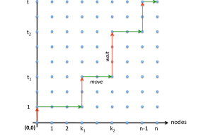
(a) CuT model.

(b) SoA model.

Figure 1: Analyzing the latency in Markov path graphs.

The probability of path $P$ conditioned on $k_{1}>0$ is the same. A path with exactly $m$ right-bends can be generated by independently choosing $m-1$ right-bending points on the space axis (the first is at $k=0$) and $m$ points on the time axes, ${n-1\choose m-1}$ and ${t\choose m}$ ways respectively, for a total of ${n-1\choose m-1}{t\choose m}$ such paths. Then the latency probability distribution $\Pr(T=t)$ for $p>0,q>0$ is given by:

$$\Pr(T=t)=\sum_{m=1}^{\min\{n,t+1\}}{n-1\choose m-1}{t-D\choose m}\frac{p^{n}q^{m}(1-p)^{t-D-m}}{(p+q)^{n}}$$ (1)

4 The Markov model with initial configuration

Let $X_{i}(t)\in\{0,1\}$ be the state of link $i$ at time $t$, where $X_{i}(t)=1$ (resp. $X_{i}(t)=0$) if link ${i}$ is on (resp. off) at time $t$, and let $X(0)=x=(x_{1},\ldots,x_{n})\in\{0,1\}^{n}$ be the initial link state, at time 0. The probability transition matrix $P_{i}$ for link ${i}$ is given by

$$P=\left(\begin{array}[]{ll}1-p&p\\ q&1-q\end{array}\right)$$

with $p$ (resp. $q$) the transition probability that link ${i}$ jumps from state $0$ (resp. state $1$) into state $1$ (resp. state $0$) in one timestep. Let $P_{a,b}({i},t)=\Pr(X_{i}(t)=b\,|\,X_{i}(0)=a)$ be the probability that link ${i}$ is in state $b\in\{0,1\}$ at time $t$ given that it was in state $a\in\{0,1\}$ at time $t=0$. Note that $P_{a,b}(t)$ does not depend on the link’s identity since all links are assumed to have the same parameters $p$ and $q$. Let $\beta=1-p-q\in[-1,1]$. It is known [5] that

$$P_{1,0}(t) = \pi_{0}(1-\beta^{t}),\quad P_{1,1}(t)=\pi_{1}+\pi_{0}\beta^{t}$$ (2)

$$P_{0,1}(t) = \pi_{1}(1-\beta^{t}),\quad P_{0,0}(t)=\pi_{0}+\pi_{1}\beta^{t}$$ (3)

for any $t\geq 0$, where $\pi_{0}=q/(p+q)$ and $\pi_{1}=p/(p+q)$ are the stationary probabilities that link $i$ is in states $0$ and in $1$, respectively.

Let $T_{i}$ be the time at which the packet reaches link ${i}$, i.e. the time at which it finishes crossing link ${i}-1$. Let $D_{i}=T_{{i}+1}-T_{i}$ be the time spent waiting for link ${i}$ to appear plus the time taken to cross it. To compute $\mathbb{E}[T_{n}]$, we begin by computing the probability generating function (PGF) of $T_{i}$, namely, $G_{{i},x}(z)=\mathbb{E}[z^{T_{i}}|X(0)=x]$ and for initial link state $x=(x_{1},\ldots,x_{n})$ and ${i}={n}$. Let

$$F_{i,1}(z)=\mathbb{E}\left[z^{D_{i}}\,|\,X_{i}(T_{{i}-1})=1\right],\quad F_{i,0}(z)=\mathbb{E}\left[z^{D_{i}}\,|\,X_{i}(T_{{i}-1})=0\right]$$

be the probability generating function (PGF) of $D_{i}$ given that link ${i}$ was in state $1$ (resp. state $0$) at time $T_{{i}-1}$, respectively, and define for all links $i\in\{1,2,\ldots,n\}$,

$$\gamma_{i,1}=\mathbb{E}[D_{i}\,|\,X_{i}(T_{{i}-1})=1],\quad\gamma_{i,0}=\mathbb{E}[D_{i}\,|\,X_{i}(T_{{i}-1})=0]$$

Note that $\gamma_{i,1}=dF_{i,1}(z)/dz|_{z=1}$ and $\gamma_{i,0}=dF_{i,0}(z)/dz|_{z=1}$.

The computation for the three edge failure models given in Sec. 2 will differ only according to the expressions for $F_{i,0}(z)$ and $F_{i,1}(z)$, which we derive expressions for below. For any number $a\in[0,1]$ let $\bar{a}=1-a$. Note that expressions of the form $a\alpha+\bar{a}\beta$ are equivalent to $\alpha\textbf{~{}if~{}}a=1\textbf{~{}else~{}}\beta$.

4.1 Computing the PGFs and the ETT

Theorem 4.1 (Computing $G_{{i},x}(z)$)

For initial state $X(0)=x=(x_{1},\ldots,x_{n})$, we can, given the values $F_{i,0}(\beta^{i}),F_{i,1}(\beta^{i})$ for ${i}$ from 0 to ${n}-1$ (each of which can be found in constant time by the computations in the following section), compute the following in $O({n}^{2})$ time:

$$G_{1,x}(z) = x_{1}F_{1,1}(z)+\bar{x}_{1}F_{1,0}(z)$$

$$G_{{i},x}(z) = \phi_{i}(z)\cdot G_{{i}-1,x}(z)+\chi({i})\cdot\psi_{i}(z)\cdot G_{{i}-1,x}(\beta z),\quad{i}=2,\ldots,{n}$$

where

$$\phi_{i}(z)=\pi_{0}F_{i,0}(z)+\pi_{1}F_{i,1}(z),\quad\psi_{i}(z)=F_{i,0}(z)-F_{i,1}(z),\quad\chi({i})=\bar{x}_{i}\pi_{1}-x_{i}\pi_{0}$$ (4)

Proof: We prove correctness recursively. The base case ($i=1$) follows immediately from the fact that $T_{1}=D_{1}$. We now show, for expository reasons, that (4.1) holds for ${i}=2$. We have:

$$G_{2,x}(z) = \sum_{t=0}^{\infty}z^{t}\mathbb{E}\bigl{[}z^{D_{2}}|X(0)=x,D_{1}=t\bigr{]}\Pr(D_{1}=t|X(0)=x)$$ (5)

$$= \sum_{t=0}^{\infty}z^{t}\sum_{j\in\{0,1\}}\mathbb{E}\left[z^{D_{2}}|X(0)=x,D_{1}=t,X_{2}(t)=j\right]\times\Pr(X_{2}(t)=j|X(0)=x,D_{1}=t)$$

$$\mbox{}\times\Pr(D_{1}=t|X(0)=x)$$

$$= \sum_{t=0}^{\infty}z^{t}(F_{2,0}(z)\Pr(X_{2}(t)=0|X(0)=x,D_{1}=t)+F_{2,1}(z)\Pr(X_{2}(t)=1|X(0)=x,D_{1}=t))$$

$$\mbox{}\times\Pr(D_{1}=t|X(0)=x)$$

$$= \sum_{t=0}^{\infty}z^{t}\phi_{2}(z)\Pr(D_{1}=t|X(0)=x)+\sum_{t=0}^{\infty}z^{t}\beta^{t}\cdot\chi(2)\cdot\psi_{2}(z)\Pr(D_{1}=t|X(0)=x)$$

$$= \phi_{2}(z)\cdot G_{1,x}(z)+\chi(2)\cdot\psi_{2}(z)\cdot G_{1,x}(\beta z)$$

where we have used (2) and (3) to derive (5).

Assume for induction that (4.1) holds for ${i}=2,\ldots,m$. We now show that it holds for ${i}=m+1$:

$$G_{m+1,x}(z)$$ (6)

$$= \sum_{t_{1}=0}^{\infty}\cdots\sum_{t_{m}=0}^{\infty}z^{\sum_{i=1}^{m}t_{i}}\mathbb{E}\left[z^{D_{m}}|X(0)=x,D_{1}=t_{1},\ldots,D_{m}=t_{m}\right]\times\Pr(D_{1}=t_{1},\ldots,D_{m}=t_{m}|X(0)=x)$$

$$= \sum_{t_{1}=0}^{\infty}\cdots\sum_{t_{m}=0}^{\infty}z^{\sum_{i=1}^{m}t_{i}}\sum_{j\in\{0,1\}}\mathbb{E}\left[z^{D_{m}}|X(0)=x,D_{1}=t_{1},\ldots,D_{m}=t_{m},X_{m+1}\Big{(}\sum_{k=1}^{m}t_{k}\Big{)}=j\right]$$

$$\times\Pr(X_{m+1}\Big{(}\sum_{k=1}^{m}t_{k}\Big{)}=j|X_{m+1}(0)=x_{m+1})\cdot\Pr(D_{1}=t_{1},\ldots,D_{m}=t_{m}|X(0)=x)$$

$$= \sum_{t_{1}=0}^{\infty}\cdots\sum_{t_{m}=0}^{\infty}z^{\sum_{i=1}^{m}t_{i}}(\phi_{m+1}(z)+\beta^{\sum_{i=1}^{m}t_{i}}\cdot\chi(m+1)\cdot\psi_{m+1}(z))$$

$$\times\Pr(D_{1}=t_{1},\ldots,D_{m}=t_{m}|X(0)=x)$$

$$= \phi_{m+1}(z)\cdot G_{m,x}(z)+\chi(m+1)\cdot\psi_{m+1}(z)\cdot G_{m,x}(\beta z)$$ (7)

where (6) follows from (2) and (3) and (7) follows from the definition of PGF.

For complexity, observe that we must compute $G_{{i},x}(\beta^{k})$ for ${i}$ from 1 to ${n}$ and $k$ from 0 to ${n}-1$, and that each such computation is done in constant time. $\Box$

Corollary 4.1 (Computing ETT)

For initial state $x=(x_{1},\ldots,x_{n})$, we can (again given the $O(1)$-time computable values $F_{i,0}(\beta^{j}),F_{i,1}(\beta^{j})$ for ${i}$ from 1 to ${n}$ and $j$ from 0 to $n-1$) compute ETT in $O({n}^{2})$ time:

$$\overline{T}_{n}(x)=\sum_{{i}=1}^{{n}}\pi_{0}\gamma_{i,0}+\pi_{1}\gamma_{i,1}+(\gamma_{i,0}-\gamma_{i,1})\cdot\chi(i)\cdot G_{i-1,x}(\beta)$$ (8)

Proof: Computing $G_{{i},x}(z)$ for all ${i}$ is done by Theorem 4.1 in $O({n}^{2})$ total time. The only additional computation time here is $O({n})$. From this, any statistic of $T_{i}$ can be obtained. Consider:

$$\overline{T}_{i}(x)=\mathbb{E}[T_{i}|X(0)=x]$$ (9)

the expected transmission time on links $1,\ldots,{i}$ given that the system is in state $x$ at time $t=0$.

Observe that $\overline{T}_{i}(x)=G^{\prime}_{{i},x}(1)$. (By convention, $G_{0,x}(z)=1$.) We then obtain the recursion (using the fact that $\phi_{i}(1)=\pi_{0}+\pi_{1}=1$, $\psi_{i}(1)=F_{i,0}(1)-F_{i,1}(1)=0$, and $G_{i-1}(1)=1$):

$$\overline{T}_{1}(x) = x_{1}\gamma_{1,1}+\bar{x}_{1}\gamma_{1,0}$$

$$\overline{T}_{i}(x) = \overline{T}_{{i}-1}(x)+\pi_{0}\gamma_{i,0}+\pi_{1}\gamma_{i,1}+(\gamma_{i,0}-\gamma_{i,1})\cdot\chi(i)\cdot G_{i-1,x}(\beta),\quad i=2,\ldots,{n}$$

which in closed form is (8). $\Box$

Observation 4.1 (Computing the probability distribution)

Since the entire probability distribution of $T_{n}(x)$ is captured by the PGF, $G_{n,x}(z)$, it is possible to retrieve the probability distribution of $T_{n}(x)$ by taking repeated derivatives as follows [3]:

$$\Pr(T_{n}(x)=k)=\frac{G_{n,x}^{(k)}(0)}{k!}$$

While computing these may not be feasible in closed form in general, it is easy to perform this computation numerically.

4.2 Computing $F_{i,1}(z)$ and $F_{i,0}(z)$

Now that the PGF of $T_{i}$ has been computed, in order to solve various link failure models, we need to compute the PGFs of $D_{i}$ as well, i.e. $F_{i,1}(z)$ and $F_{i,0}(z)$. Let $S$ be the random variable (rv) denoting the time needed to traverse a link and $Y$ be the rv denoting the amount of time spent waiting, upon arrival there, for the link to turn on. First observe that for all links $i\in\{1,2,\ldots,n\}$:

$$F_{i,0}(z)=G_{Y}(z)F_{i,1}(z)$$ (10)

since $D_{i}|_{X_{i}(T_{{i}})=0}=_{d}Y+D_{i}|_{X_{i}(T_{{i}})=1}$, ($=_{d}$ indicates equality in distribution) where $Y$ is a geometrically distributed rv with parameter $p$, independent of $D_{i}|_{X_{i}(T_{{i}})=1}$. (A sum of rv’s yields a product of PGFs.) In our model, since $Y$ corresponds to the duration of an off period of a link, $\Pr(Y=k)=(1-p)^{k-1}p$ which yields the following PGF:

$$G_{Y}(z)=\frac{pz}{1-(1-p)z},\quad 0\leq|z|\leq 1$$ (11)

Lemma 4.1

For the case of geometrically distributed link off periods (Y), $\gamma_{0}=\gamma_{1}+\frac{1}{p}$

Proof: Recall that $\gamma_{i,1}=dF_{i,1}(z)/dz|_{z=1}$ and $\gamma_{i,0}=dF_{i,0}(z)/dz|_{z=1}$ and $F_{i,0}(z)=G_{Y}(z)F_{i,1}(z)$. It is easy to see that $G_{Y}(1)=1$ and $dG_{Y}(z)/dz|_{z=1}=\frac{1}{p}$, whereas $F_{i,1}(1)=\mathbb{E}\left[1\,|\,X_{i}(T_{{i}})=1\right]=1$. In this case, we have:

$$\gamma_{i,0} = dF_{i,0}(z)/dz|_{z=1}$$

$$= dG_{Y}(z)/dz|_{z=1}*F_{i,1}(1)+G_{Y}(1)*dF_{i,1}(z)/dz|_{z=1}$$

$$= 1/p+\gamma_{i,1}$$

$\Box$

4.2.1 Failure model 3: complete retransmission after link failure

We consider two subcases:

• Successive retransmission times on a link are all identical, denoted by the rv $S$.

• Successive retransmission times on a link are iid rvs $\{S,S_{1},S_{2}\ldots,\}$.

Let $G_{S}(z)$ be the PGF of $S$. Throughout $\{W,W_{1},W_{2},\ldots\}$ and $\{Y,Y_{1},Y_{2},\ldots\}$ are assumed to be independent sequences of iid rvs, furthermore independent of $S$ in case (a) and of $\{S,S_{1},S_{2}\ldots,\}$ in case (b), that are geometrically distributed with parameters $q$ and $p$, respectively. The rv $W_{i}$ (resp. $Y_{i}$) corresponds to the $i$th on period (resp. off period) of a link since the first attempt to transmit the packet. Let ${\bf 1}_{A}$ be the indicator function of the event $A$. Also, in the subsequent text, the subscript $i$ is implicit in the expressions involving $F_{0}(z),F_{1}(z)$ for notational convenience.

Case (a):

Conditioned on $X(T_{{i}})=1$, we have

$$D_{i}=_{d}\sum_{i\geq 0}{\bf 1}_{A_{i}(S)}\left(S+\sum_{l=1}^{i}(W_{l}+Y_{l})\right)$$

with $A_{i}(u)=\{W_{1}<u,\ldots,W_{i}<u,W_{i+1}\geq u\}$. Note that $A_{i}(u)\cap A_{j}(u)=\emptyset$ for $i\not=j$ and $\sum_{i\geq 0}\Pr(A_{i}(u))=1$, for any $u$. We have

$$F_{1}(z) = \sum_{u=0}^{\infty}\mathbb{E}\left[z^{\bigl{(}\sum_{i\geq 0}{\bf 1}_{A_{i}(u)}\bigl{(}u+\sum_{l=1}^{i}(W_{l}+Y_{l})\bigr{)}\bigr{)}}\,\Bigl{|}\,S=u\right]\Pr(S=u)$$

$$= \sum_{u=0}^{\infty}\Pr(S=u)z^{u}\sum_{i=0}^{\infty}\mathbb{E}\left[z^{\bigl{(}\sum_{l=1}^{i}(W_{l}+Y_{l})\bigr{)}}\,|\,S=u,A_{i}(u)=1\right]\Pr(A_{i}(u)=1|S=u)$$

$$= \Pr(S=0)+\sum_{u=1}^{\infty}\Pr(S=u)z^{u}\Pr(W\geq u)\sum_{i=0}^{\infty}G_{Y}(z)^{i}\mathbb{E}[z^{W}|W<u]^{i}\Pr(W<u)^{i}$$

$$= \Pr(S=0)+\frac{1}{1-q}\sum_{u=1}^{\infty}\frac{\Pr(S=u)((1-q)z)^{u}}{1-G_{Y}(z)\mathbb{E}[z^{W}|W<u]\Pr(W<u)}.$$

The latter identity follows from $\Pr(W=i)=(1-q)^{i-1}q$, $i\geq 1$, which yields

$$\Pr(W\geq u)=q\sum_{i=u-1}^{\infty}(1-q)^{i}=q\left(\sum_{i=0}^{\infty}(1-q)^{i}-\sum_{i=0}^{u-2}(1-q)^{i}\right)=(1-q)^{u-1},\quad u\geq 1$$

On the other hand, for $u\geq 1$,

$$\mathbb{E}[z^{W}|W<u]\Pr(W<u)=\sum_{i=1}^{u-1}E[z^{W}|W<u,W=i]\Pr(W=i|W<u)\Pr(W<u)$$

$$= \sum_{i=1}^{u-1}z^{i}\Pr(W=i)=qz\sum_{i=0}^{u-2}((1-q)z)^{i}=qz\frac{1-((1-q)z)^{u-1}}{1-(1-q)z},$$

so that

$$F_{1}(z) = \Pr(S=0)+\frac{(1-(1-p)z)(1-(1-q)z)}{1-q}$$

$$\times\sum_{u=1}^{\infty}\frac{\Pr(S=u)((1-q)z)^{u}}{(1-(1-p)z)(1-(1-q)z)-pqz^{2}(1-((1-q)z)^{u-1})}$$

by using (11). From (10) we deduce

$$F_{0}(z) = \Pr(S=0)+pz\,\frac{1-(1-q)z}{1-q}\times\sum_{u=1}^{\infty}\frac{\Pr(S=u)((1-q)z)^{u}}{(1-(1-p)z)(1-(1-q)z)-pqz^{2}(1-((1-q)z)^{u-1})}$$

If $S=1$ (i.e., SoA), we have

$$F_{0}(z)=\frac{pz^{2}}{1-(1-p)z},\quad F_{1}(z)=z$$

And if $S=0$ (i.e., CuT), we have

$$F_{0}(z)=\frac{pz}{1-(1-p)z},\quad F_{1}(z)=1$$

Case (b):

Conditioned on $X(T_{{i}})=1$, we have

$$D_{i}=_{d}\sum_{i\geq 0}{\bf 1}_{B_{i}(S_{1},\ldots,S_{i+1})}\left(S_{i+1}+\sum_{l=1}^{i}(W_{l}+Y_{l})\right)$$

with $B_{i}(u_{1},\ldots,u_{i+1})=\{W_{1}<u_{1},\ldots,W_{i}<u_{i},W_{i+1}\geq u_{i+1}\}$. Hence,

$$F_{1}(z) = \sum_{i=0}^{\infty}\Pr(B_{i}(S_{1},\ldots,S_{i})=1)\mathbb{E}\left[z^{(S_{i+1}+\sum_{l=1}^{i}(W_{l}+Y_{l}))}\,|\,B_{i}(S_{1},\ldots,S_{i})=1\right]$$ (12)

$$= \sum_{i=0}^{\infty}\Pr(W<R)^{i}\Pr(W\geq S)Y(z)^{i}\mathbb{E}\left[z^{(S_{i+1}+\sum_{l=1}^{i}W_{l})}\,|\,S_{1}>W_{1},\ldots,S_{i}>W_{i},S_{i+1}\leq W_{i+1}\right]$$

$$= \sum_{i=0}^{\infty}G_{Y}(z)^{i}(\Pr(W<S)\mathbb{E}[z^{W}|W<S])^{i}\Pr(W\geq S)\mathbb{E}[z^{S}|W\geq S]$$

$$= \frac{\Pr(W\geq S)\mathbb{E}[z^{S}|W\geq S]}{1-G_{Y}(z)\Pr(W<S)\mathbb{E}[z^{W}|W<S]}$$

Let us concentrate on $\mathbb{E}[z^{S}|W\geq S]\Pr(W\geq S)$ and $\mathbb{E}[z^{W}|W<S]\Pr(W<S)$:

$$\mathbb{E}[z^{S}|W\geq S] = \sum_{u=0}^{\infty}z^{u}\Pr(S=u|W\geq S)=\frac{\Pr(S=0)+\sum_{u=1}^{\infty}z^{u}\Pr(S=u)\Pr(W\geq u)}{\Pr(W\geq S)}$$

$$= \frac{\Pr(S=0)+\sum_{u=1}^{\infty}z^{u}\Pr(S=u)(1-q)^{u-1}}{\Pr(W\geq S)}=\frac{(G_{S}((1-q)z)-q\Pr(S=0))}{(1-q)\Pr(W\geq S)}$$

or

$$\mathbb{E}[z^{S}|W\geq S]\Pr(W\geq S)=\frac{(G_{S}((1-q)z)-p\Pr(S=0))}{(1-q)}$$

and

$$\mathbb{E}[z^{W}|W<S]\Pr(W<S) = \Pr(W<S)\sum_{w=1}^{\infty}z^{w}\Pr(W=w|W<S)$$

$$= \sum_{w=1}^{\infty}z^{w}\Pr(W=w)\Pr(S>w)=qz\sum_{w=1}^{\infty}((1-q)z)^{w-1}\sum_{u=w+1}^{\infty}\Pr(S=u)$$

$$= qz\sum_{u=2}^{\infty}\Pr(S=u)\sum_{w=1}^{u-1}((1-q)z)^{w-1}=qz\sum_{u=2}^{\infty}\Pr(S=u)\frac{1-((1-q)z)^{u-1}}{1-(1-q)z}$$

$$= \frac{q(G_{S}((1-q)z)-\Pr(S=0)-\Pr(S=1)(1-q)z))}{(1-q)(1-(1-q)z)}$$

Substituting into (12) yields:

$$F_{1}(z)=\frac{(G_{S}((1-q)z)-q\Pr(S=0))(1-(1-q)z)(1-(1-p)z)}{(1-(1-p)z)(1-(1-q)z)(\Pr(S=0)+\Pr(S=1)(1-q)z-G_{S}((1-q)z))}$$

4.2.2 Failure model 2: transmission is resumed after link failure

Let us compute $F_{1}(z)$. Conditioned on $X(T_{{i}})=1$, we have $D_{i}=S+\sum_{l=1}^{V}Y_{l}$, where $V$ is a binomial rv with parameter $q$ and population $S-1$. Note that given a population $S=u+1$, $G_{V}(z)=1-q(1-z))^{u}$. If a sum of rv’s $Z=X_{1}+X_{2}+\cdots+X_{N}$ where $X_{i}$’s are iid rv’s and $N$ is also a rv, then $G_{Z}(z)=G_{N}(G_{X}(z))$ [3]. Hence we can write:

$$F_{1}(z) = \Pr(S=0)+\sum_{u=1}^{\infty}\Pr(S=u)z^{u}[1-q(1-G_{Y}(z))]^{u-1}$$

$$= \frac{G_{S}(1-q(1-G_{Y}(z)))-\Pr(S=0)q(1-Y(z))}{1-q(1-G_{Y}(z))}$$

$$F_{0}(z) = G_{Y}(z)\frac{G_{S}(1-q(1-G_{Y}(z)))-\Pr(S=0)q(1-G_{Y}(z))}{1-q(1-G_{Y}(z))}$$

4.2.3 Failure model 1: already started transmission is unaffected by link failure

This is by far the simplest scenario:

$$F_{1}(z)=G_{S}(z),\quad F_{0}(z)=G_{Y}(z)G_{S}(z)$$

5 Discussion and future work

In this paper we exactly computed the expected time to traverse a dynamic path with edge states governed by Markov chains. Natural interesting generalizations include edge failures that are not independent; for example, adjacent pairs of edge failures would correspond to a node failure, and probability $q_{i},p_{i}$ that vary by link. Our algorithms maintain the same complexity as long as $p_{i}+q_{i}$ is constant, but in the full generalization become exponential-time. These techniques have applications in modeling communication along military convoys traveling through rugged terrain, and sensor network-based monitoring of linear civil structures such as bridges or trains.

References

• [1] K. Argyraki and D. R. Cheriton. Loose source routing as a mechanism for traffic policies. In Proceedings of the ACM SIGCOMM workshop on Future directions in network architecture, FDNA ’04, pages 57–64, New York, NY, USA, 2004. ACM.
• [2] B. Eisenberg. On the expectation of the maximum of iid geometric random variables. Statistics and Probability Letters, 78:135–143, 2008.
• [3] G. Grimmett and D. Welsh. Probability: An Introduction. Oxford University Press, 1986.
• [4] D. B. Johnson, D. A. Maltz, and J. Broch. DSR: The Dynamic Source Routing Protocol for Multi-Hop Wireless Ad Hoc Networks, volume Ad Hoc Networking, chapter 5, pages 139–172. Addison-Wesley, 2001. Editor: Charles E. Perkins.
• [5] D. A. Levin, Y. Peres, and E. L. Wilmer. Markov Chains and Mixing Times. American Mathematical Society, 2008.
• [6] R. Ramanathan. Challenges: A radically new architecture for next generation mobile ad hoc networks. In Proc. of MOBICOM, Cologne, Germany, August 2005.
• [7] W. Szpankowski and V. Rego. Yet another application of binomial recurrence: order statistics. Computing, 43:401 410, 1990.