From propositional to first-order monitoring

Abstract

The main purpose of this paper is to introduce a first-order temporal logic, $\operatorname{LTL}^{\hbox{\tiny{$\operatorname{FO}$}}}$, and a corresponding monitor construction based on a new type of automaton, called spawning automaton.

Specifically, we show that monitoring a specification in $\operatorname{LTL}^{\hbox{\tiny{$\operatorname{FO}$}}}$ boils down to an undecidable decision problem. The proof of this result revolves around specific ideas on what we consider a “proper” monitor. As these ideas are general, we outline them first in the setting of standard LTL, before lifting them to the setting of first-order logic and $\operatorname{LTL}^{\hbox{\tiny{$\operatorname{FO}$}}}$. Although due to the above result one cannot hope to obtain a complete monitor for $\operatorname{LTL}^{\hbox{\tiny{$\operatorname{FO}$}}}$, we prove the soundness of our automata-based construction and give experimental results from an implementation. These seem to substantiate our hypothesis that the automata-based construction leads to efficient runtime monitors whose size does not grow with increasing trace lengths (as is often observed in similar approaches). However, we also discuss formulae for which growth is unavoidable, irrespective of the chosen monitoring approach.

1 Introduction

In the area of runtime verification (cf. [14, 13, 9, 6]), a monitor typically describes a device or program which is automatically generated from a formal specification capturing undesired (resp. desired) system behaviour. The monitor’s task is to passively observe a running system in order to detect if the behavioural specification has been satisfied or violated by the observed system behaviour. While, arguably, the majority of runtime verification approaches are based on propositional logic, there exist works that also consider first-order logic (cf. [13, 4, 3]). Monitoring first-order specifications has also gained prior attention in the database community, especially in the context of so called temporal triggers, which correspond to first-order temporal logic specifications that are evaluated wrt. a linear sequence of database updates (cf. [7, 8, 19]). Although the underlying logics are generally undecidable, the monitors in these works usually address decidable problems, such as “is the observed behaviour so far a violation of a given specification $\varphi$?” Additionally, in many approaches, $\varphi$ must only ever be a safety or domain independent property for this problem to actually be decidable (cf. [7, 3]), which can be ensured by syntactic restrictions on the input formula, for example.

As there exist many different ways in which a system can be monitored in this abstract sense, we are going to put forth very specific assumptions concerning the properties and inner-workings of what we consider a “proper” monitor. None of these assumptions is particularly novel or complicated, but they help describe and distinguish the task of a “proper” monitor from that of, say, a model checker, which can also be used to solve monitoring problems as we shall see.

The two basic assumptions are easy to explain: Firstly, we demand that a monitor is what we call trace-length independent, meaning that its efficiency does not decline with an increasing number of observations. Secondly, we demand that a monitor is monotonic wrt. reporting violations (resp. satisfication) of a specification, meaning that once the monitor returns “SAT” to the user, additional observations do not lead to it returning “UNSAT” (and vice versa). We are going to postulate further assumptions, but these are mere consequences of the two basic ones, and are explained in §2.

At the heart of this paper, however, is a custom first-order temporal logic, in the following referred to as $\operatorname{LTL}^{\hbox{\tiny{$\operatorname{FO}$}}}$, which is undecidable. Yet we outline a sound, albeit incomplete, monitor construction for it based on a new type of automaton, called spawning automaton. $\operatorname{LTL}^{\hbox{\tiny{$\operatorname{FO}$}}}$ was originally developed for the specification of runtime verification properties of Android “Apps” and has already been used in that context (see [5] for details). Although [5] gave a monitoring algorithm for $\operatorname{LTL}^{\hbox{\tiny{$\operatorname{FO}$}}}$ based on formula rewriting, it turns out that the automata-based construction given in this paper leads to practically more efficient results.

As our definition of what constitutes a “proper” monitor is not tied to a particular logic we will develop it first for standard LTL (§2), the quasi-standard in the area of runtime verification. In §3, we give a more detailed account of $\operatorname{LTL}^{\hbox{\tiny{$\operatorname{FO}$}}}$ than was available in [5], before we lift the results of §2 to the first-order setting (§4). The automata-based monitor construction for $\operatorname{LTL}^{\hbox{\tiny{$\operatorname{FO}$}}}$ along with experimental results is described in §5. Related work is discussed in §6. Detailed proofs can be found in a separate appendix.

2 Complexity of monitoring in the propositional case

In what follows, we assume basic familiarity with $\operatorname{LTL}$ and topics like model checking (cf. [2] for an overview). Despite that, let us first state a formal $\operatorname{LTL}$ semantics, since we will consider its interpretation on infinite and finite traces. For that purpose, let $\operatorname{AP}$ denote a set of propositions, $\operatorname{LTL}(\operatorname{AP})$ the set of well-formed LTL formulae over that set, and for some set $X$ set $X^{\infty}=X^{\omega}\cup X^{\ast}$ to be the union of the set of all infinite and finite traces over $X$. When $\operatorname{AP}$ is clear from the context, or does not matter, we use $\operatorname{LTL}$ instead of $\operatorname{LTL}(\operatorname{AP})$. Also, for a given trace $w=w_{0}w_{1}\ldots$, the trace $w^{i}$ is defined as $w_{i}w_{i+1}\ldots$. As a convention we use $u,u^{\prime},\ldots$ to denote finite traces, by $\sigma$ the trace of length $1$, and $w$ for infinite ones or where the distinction is of no relevance.

Definition 1

Let $\varphi\in\operatorname{LTL}(\operatorname{AP})$, $w\in(2^{\operatorname{AP}})^{\infty}$ be a non-empty trace, and $i\in\mathbb{N}_{0}$, then

$$\begin{array}[]{rcl}w^{i}\models p&\hbox{ iff }&p\in w_{i},\hbox{ where }p\in\operatorname{AP},\\ w^{i}\models\neg\varphi&\hbox{ iff }&w^{i}\models\varphi\hbox{ does not hold},\\ w^{i}\models\varphi\wedge\psi&\hbox{ iff }&w^{i}\models\varphi\hbox{ and }w^{i}\models\psi,\\ w^{i}\models\mathsf{X}\varphi&\hbox{ iff }&|w|>i\hbox{ and }w^{i+1}\models\varphi,\\ w^{i}\models\varphi\mathsf{U}\psi&\hbox{ iff }&\hbox{there is a }k\hbox{ s.t. }i\leq k\leq|w|,w^{k}\models\psi,\hbox{ and for all }i\leq j<k,w^{j}\models\varphi.\end{array}$$

And if $w^{0}\models\varphi$ holds, we usually write $w\models\varphi$ instead. Although this semantics, which was also proposed in [17], gives rise to mixed languages, i.e., languages consisting of finite and infinite traces, we shall only ever be concerning ourselves with either finite-trace or infinite-trace languages, but not mixed ones. It is easy to see that over infinite traces this semantics matches the definition of standard $\operatorname{LTL}$. Recall, $\operatorname{LTL}$ is a decidable logic; in fact, the satisfiability problem for $\operatorname{LTL}$ is known to be PSpace-complete [18].

As there are no commonly accepted rules for what qualifies as a monitor (not even in the runtime verification community), there exist a myriad of different approaches to checking that an observed behaviour satisfies (resp. violates) a formal specification, such as an $\operatorname{LTL}$ formula. Some of these (cf. [14, 4]) consist in solving the word problem (see Definition 2). A monitor following this idea can either first record the entire system behaviour in form of a trace $u\in\Sigma^{+}$, where $\Sigma$ is a finite alphabet of events, or process the events incrementally as they are emitted by the system under scrutiny. Both approaches are documented in the literature (cf. [14, 12, 13, 4]), but only the second one is suitable to detect property violations (resp. satisfaction) right when they occur.

Definition 2

The word problem for $\operatorname{LTL}$ is defined as follows.

Input: A formula $\varphi\in\operatorname{LTL}(\operatorname{AP})$ and some trace $u\in(2^{\operatorname{AP}})^{+}$.

Question: Does $u\models\varphi$ hold?

In [17] a bilinear algorithm for this problem was presented (an even more efficient solution was recently given in [15]). Hence, the first sort of monitor, which is really more of a test oracle than a monitor, solves a classical decision problem. The second monitor, however, solves an entirely different kind of problem, which cannot be stated in complexity-theoretical terms at all: its input is an $\operatorname{LTL}$ formula and a finite albeit unbounded trace which grows incrementally. This means that this monitor solves the word problem for each and every new event that is added to the trace at runtime. We can therefore say that the word problem acts as a lower bound on the complexity of the monitoring problem that such a monitor solves; or, in other words, the problem that the online monitor solves is at least as hard as the problem that the offline monitor solves.

There are approaches to build efficient (i.e., trace-length independent) monitors that repeatedly answer the word problem (cf. [14]). However, such approaches violate our second basic assumption, mentioned in the introduction of this paper, in that they are necessarily non-monotonic. To see this, consider $\varphi=a\mathsf{U}b$ and some trace $u=\{a\}\{a\}\ldots\{a\}$ of length $n$. Using our finite-trace interpretation, $u\not\models\varphi$. However, if we add $u_{n+1}=\{b\}$, we get $u\models\varphi$. For the user, this essentially means that she cannot trust the verdict of the monitor as it may flip in the future, unless of course it is obvious from the start that, e.g., only safety properties are monitored and the monitor is built merely to detect violations, i.e., bad prefixes. However, if we take other monitorable languages into account as we do in this paper, i.e., those that have either good or bad prefixes (or both), we need to distinguish between satisfaction and violation of a property (and want the monitor to report either occurrence truthfully).

Definition 3

For any $L\subseteq\Sigma^{\omega}$, $u\in\Sigma^{\ast}$ is called a good prefix (resp. bad prefix) iff $u\Sigma^{\omega}\subseteq L$ holds (resp. $u\Sigma^{\omega}\cap L=\emptyset$).

We shall use $\operatorname{good}(L)\subseteq\Sigma^{\ast}$ (resp. $\operatorname{bad}(L)$) to denote the set of good (resp. bad) prefixes of $L$. For brevity, we also write $\operatorname{good}(\varphi)$ instead of $\operatorname{good}(\mathcal{L}(\varphi))$, and do the same for $\operatorname{bad}(\mathcal{L}(\varphi))$.

A monitor that detects good (resp. bad) prefixes has been termed anticipatory in [9] as it not only states something about the past, but also about the future: once a good (resp. bad) prefix has been detected, no matter how the system would evolve in an indefinite future, the property would remain satisfied (resp. violated). In that sense, anticipatory monitors are monotonic by definition. Moreover in [6], a construction is given, showing how to obtain trace-length independent (even optimal) anticipatory monitors for $\operatorname{LTL}$ and a timed extension called TLTL. The obtained monitor basically returns $\top$ to the user if $u\in\operatorname{good}(\varphi)$ holds, $\bot$ if $u\in\operatorname{bad}(\varphi)$ holds, and $?$ otherwise. Not surprisingly though, the monitoring problem such a monitor solves is computationally more involved than the word problem. It solves what we call the prefix problem (of $\operatorname{LTL}$), which can easily be shown PSpace-complete by way of $\operatorname{LTL}$ satisfiability.

Definition 4

The prefix problem for $\operatorname{LTL}$ is defined as follows.

Input: A formula $\varphi\in\operatorname{LTL}(\operatorname{AP})$ and some trace $u\in(2^{\operatorname{AP}})^{\ast}$.

Question: Does $u\in\operatorname{good}(\varphi)$ (resp. $\operatorname{bad}(\varphi)$) hold?

Theorem 2.1

The prefix problem for $\operatorname{LTL}$ is PSpace-complete.

Proof

For brevity, we will only show the theorem for bad prefixes. It is easy to see that $u\in\operatorname{bad}(\varphi)$ iff $\mathcal{L}(u_{0}\wedge\mathsf{X}u_{1}\wedge\mathsf{X}\mathsf{X}u_{2}\wedge\ldots\wedge\varphi)=\emptyset$. Constructing this conjunction takes only polynomial time and the corresponding emptiness check can be performed in PSpace [18]. To show hardness, we proceed with a reduction of LTL satisfiability. Again, it is easy to see that $\mathcal{L}(\varphi)\neq\emptyset$ iff $\sigma\not\in\operatorname{bad}(\mathsf{X}\varphi)$ for any $\sigma\in 2^{\operatorname{AP}}$. This reduction is linear, and as PSpace $=$ co-PSpace, the statement follows. ∎

We would like to point out the possibility of building an anticipatory though trace-length dependent $\operatorname{LTL}$ monitor using an “off the shelf” model checker, which accepts a propositional Kripke structure and an $\operatorname{LTL}$ formula as input. Note that here we make the assumption that Kripke structures produce infinite as opposed to finite traces.

Definition 5

The model checking problem for $\operatorname{LTL}$ is defined as follows.

Input: A formula $\varphi\in\operatorname{LTL}(\operatorname{AP})$ and a Kripke structure $\mathcal{K}$ over $2^{\operatorname{AP}}$.

Question: Does $\mathcal{L}(\mathcal{K})\subseteq\mathcal{L}(\varphi)$ hold?

As in $\operatorname{LTL}$ the model checking and the satisfiability problems are both PSpace-complete [18], we can use a model checking tool as monitor: given that it is straightforward to construct $\mathcal{K}$ s.t. $\mathcal{L}(\mathcal{K})=u(2^{\operatorname{AP}})^{\omega}$ in no more than polynomial time, we return $\top$ to the user if $\mathcal{L}(\mathcal{K})\subseteq\mathcal{L}(\varphi)$ holds, $\bot$ if $\mathcal{L}(\mathcal{K})\subseteq\mathcal{L}(\neg\varphi)$ holds, and $?$ if neither holds. One could therefore be tempted to think of monitoring merely in terms of a model checking problem, but we shall see that as soon as the logic in question has an undecidable satisfiability problem this reduction fails. Besides, it can be questioned whether monitoring as model checking leads to a desirable monitor with its obvious trace-length dependence and having to repeatedly solve a PSpace-complete problem for each new event.

3 $\operatorname{LTL}^{\hbox{\tiny{$\operatorname{FO}$}}}$—Formal definitions and notation

Let us now introduce our first-order specification language $\operatorname{LTL}^{\hbox{\tiny{$\operatorname{FO}$}}}$ and related concepts in more detail. The first concept we need is that of a sorted first-order signature, given as $\Gamma=(\mathbf{S},\mathbf{F},\allowbreak\mathbf{R})$, where $\mathbf{S}$ is a finite non-empty set of sorts, $\mathbf{F}$ a finite set of function symbols and $\mathbf{R}=\mathbf{U}\cup\mathbf{I}$ a finite set of a priori uninterpreted and interpreted predicate symbols, s.t. $\mathbf{U}\cap\mathbf{I}=\emptyset$ and $\mathbf{R}\cap\mathbf{F}=\emptyset$. The former set of predicate symbols are referred to as $\mathbf{U}$-operators and the latter as $\mathbf{I}$-operators. As is common, 0-ary functions symbols are also referred to as constant symbols. We assume that all operators in $\Gamma$ have a given arity that ranges over the sorts given by $\mathbf{S}$, respectively. We also assume an infinite supply of variables, $\mathbf{V}$, that also range over $\mathbf{S}$ and where $\mathbf{V}\cap(\mathbf{F}\cup\mathbf{R})=\emptyset$. Let us refer to the first-order language determined by $\Gamma$ as $\mathcal{L}(\Gamma)$. While terms in $\mathcal{L}(\Gamma)$ are made up of variables and function symbols, formulae of $\mathcal{L}(\Gamma)$ are defined as follows:

$$\varphi::=p(t_{1},\ldots,t_{n})\mid r(t_{1},\ldots,t_{n})\mid\neg\varphi\mid\varphi\wedge\varphi\mid\mathsf{X}\varphi\mid\varphi\mathsf{U}\varphi\mid\forall(x_{1},\ldots,x_{n}):p.\ \varphi,$$

where $t_{1},\ldots,t_{n}$ are terms, $p\in\mathbf{U}$, $r\in\mathbf{I}$, and $x_{1},\ldots,x_{n}\in\mathbf{V}$. As variables are sorted, in the quantified formula $\forall(x_{1},\ldots,x_{n}):p.\ \varphi$, the $\mathbf{U}$-operator $p$ with arity $\tau_{1}\times\ldots\times\tau_{n}$, defines the sorts of variables $x_{1},\ldots,x_{n}$ to be $\tau_{1},\ldots,\tau_{n}$, with $\tau_{i}\in\mathbf{S}$, respectively. For terms $t_{1},\ldots,t_{n}$, we say that $p(t_{1},\ldots,t_{n})$ is well-sorted if the sort of every $t_{i}$ is $\tau_{i}$. This notion is inductively applicable to terms. Moreover, we consider only well-sorted formulae and refer to the set of all well-sorted $\mathcal{L}(\Gamma)$ formulae over a signature $\Gamma$ in terms of $\operatorname{LTL}^{\hbox{\tiny{$\operatorname{FO}$}}}_{\Gamma}$. When a specific $\Gamma$ is either irrelevant or clear from the context, we will simply write $\operatorname{LTL}^{\hbox{\tiny{$\operatorname{FO}$}}}$ instead. When convenient and a certain index is of no importance in the given context, we also shorten notation of a vector $(x_{1},\ldots,x_{n})$ by a (bold) $\operatorname{\vec{x}}$.

A $\Gamma$-structure, or just first-order structure is a pair $\mathfrak{A}=(|\mathfrak{A}|,I)$, where $|\mathfrak{A}|=|\mathfrak{A}|_{1}\cup\ldots\cup|\mathfrak{A}|_{n}$, is a non-empty set called domain, s.t. every sub-domain $|\mathfrak{A}|_{i}$ is either a non-empty finite or countable set (e.g., set of all integers or strings) and $I$ an interpretation. $I$ assigns to each sort $\tau_{i}\in\mathbf{S}$ a specific sub-domain $\tau_{i}^{I}=|\mathfrak{A}|_{i}$, to each constant symbol $c\in\mathbf{F}$ of sort $\tau_{i}$ a domain value $c^{I}\in|\mathfrak{A}|_{i}$, to each function symbol $f\in\mathbf{F}$ of arity $\tau_{1}\times\ldots\times\tau_{l}\longrightarrow\tau_{m}$ a function $f^{I}:|\mathfrak{A}|_{1}\times\ldots\times|\mathfrak{A}|_{l}\longrightarrow|\mathfrak{A}|_{m}$, and to every $\mathbf{I}$-operator $r$ with arity $\tau_{1}\times\ldots\times\tau_{m}$ a relation $r^{I}\subseteq|\mathfrak{A}|_{1}\times\ldots\times|\mathfrak{A}|_{m}$. We restrict ourselves to computable relations and functions. In that regard, we can think of $I$ as a mapping between $\mathbf{I}$-operators (resp. function symbols) and the corresponding algorithms which compute the desired return values, each conforming to the symbols’ respective arities. Note that the interpretation of $\mathbf{U}$-operators is rather different from $\mathbf{I}$-operators, as it is closely tied to what we call a trace and therefore discussed in more detail after we introduce the necessary notions and notation.

For the purpose of monitoring $\operatorname{LTL}^{\hbox{\tiny{$\operatorname{FO}$}}}$ specifications, we model observed system behaviour in terms of actions: Let $p\in\mathbf{U}$ with arity $\tau_{1}\times\ldots\times\tau_{m}$ and $\operatorname{\vec{d}}\in D_{p}=|\mathfrak{A}|_{1}\times\ldots\times|\mathfrak{A}|_{m}$, then we call $(p,\operatorname{\vec{d}})$ an action. We refer to finite sets of actions as events. A system’s behaviour over time is therefore a finite trace of events, which we also denote as a sequence of sets of ground terms $\{sms(1234)\}\{login(``\hbox{user}")\}\ldots$ when we mean the sequence of tuples $\{(sms,1234)\}\allowbreak\{(login,``\hbox{user}")\}\ldots$ Therefore the occurrence of some action $sms(1234)$ in the trace at position $i\in\mathbb{N}_{0}$, written $sms(1234)\in w_{i}$, indicates that at time $i$ it is the case that $sms(1234)$ holds (or, from a practical point of view, an SMS was sent to number $1234$). We follow the convention that only symbols from $\mathbf{U}$ appear in a trace, which therefore gives these symbols their respective interpretations. The following formalises this notion.

A first-order temporal structure is a tuple $(\overline{\mathfrak{A}},w)$, where $\overline{\mathfrak{A}}=(|\mathfrak{A}_{0}|,I_{0})\allowbreak(|\mathfrak{A}_{1}|,I_{1})\allowbreak\ldots$ is a (possibly infinite) sequence of first-order structures and $w=w_{0}w_{1}\ldots$ a corresponding trace. We demand that for all $\mathfrak{A}_{i}$ and $\mathfrak{A}_{i+1}$ from $\overline{\mathfrak{A}}$, it is the case that $|\mathfrak{A}_{i}|=|\mathfrak{A}_{i+1}|$, for all $f\in\mathbf{F}$, $f^{I_{i+1}}=f^{I_{i}}$, and for all $\tau\in\mathbf{S}$, $\tau^{I_{i}}=\tau^{I_{i+1}}$. For any two structures, $\mathfrak{A}$ and $\mathfrak{A}^{\prime}$, which satisfy these conditions, we write $\mathfrak{A}\sim\mathfrak{A}^{\prime}$. Moreover given some $\overline{\mathfrak{A}}$ and $\mathfrak{A}$, if for all $\mathfrak{A}_{i}$ from $\overline{\mathfrak{A}}$, we have that $\mathfrak{A}_{i}\sim\mathfrak{A}$, we also write $\overline{\mathfrak{A}}\sim\mathfrak{A}$. Finally, the interpretation of an $\mathbf{U}$-operator $p$ with arity $\tau_{1}\times\ldots\times\tau_{m}$ is then defined wrt. a position $i$ in $w$ as $p^{I_{i}}=\{\operatorname{\vec{d}}\mid(p,\operatorname{\vec{d}})\in w_{i}\}$. Essentially this means that, unlike function symbols, $\mathbf{U}$- and $\mathbf{I}$-operators don’t have to be rigid.

Note also that from this point forward, we consider only the case where the policy to be monitored is given as a closed formula, i.e., a sentence. This is closely related to our means of quantification: a quantifier in $\operatorname{LTL}^{\hbox{\tiny{$\operatorname{FO}$}}}$ is restricted to those elements that appear in the trace, and not arbitrary elements from a (possibly infinite) domain. While certain policies cannot be expressed with this restriction (e.g., “for all phone numbers $x$ that are not in the contact list, $r(x)$ is true”), this restriction bears the advantage that, when examining a given trace, functions and relations are only ever evaluated over known objects. The advantages of this type of quantification in monitoring first-order languages has also been pointed out in [13, 4]. In other words, had we allowed free variables in policies, the monitor might end up having to “try out” all the different domain elements in order to evaluate such a policy, which runs counter to our design rationale of quantification.

In what follows, let us fix a particular $\Gamma$. The semantics of $\operatorname{LTL}^{\hbox{\tiny{$\operatorname{FO}$}}}$ can now be defined wrt. a quadruple $(\overline{\mathfrak{A}},w,v,i)$ as follows, where $i\in\mathbb{N}_{0}$, and $v$ is an (initially empty) set of valuations assigning domain values to variables:

$$(\overline{\mathfrak{A}},w,v,i)\models p(t_{1},\ldots,t_{n}) \hbox{~{} iff ~{}}(t_{1}^{I_{i}},\ldots,t_{n}^{I_{i}})\in p^{I_{i}},$$

$$(\overline{\mathfrak{A}},w,v,i)\models r(t_{1},\ldots,t_{n}) \hbox{~{} iff ~{}}(t_{1}^{I_{i}},\ldots,t_{n}^{I_{i}})\in r^{I_{i}},$$

$$(\overline{\mathfrak{A}},w,v,i)\models\neg\varphi \hbox{~{} iff ~{}}(\overline{\mathfrak{A}},w,v,i)\models\varphi\hbox{ is not true},$$

$$(\overline{\mathfrak{A}},w,v,i)\models\varphi\wedge\psi \hbox{~{} iff ~{}}(\overline{\mathfrak{A}},w,v,i)\models\varphi\hbox{ and }(\overline{\mathfrak{A}},w,v,i)\models\psi,$$

$$(\overline{\mathfrak{A}},w,v,i)\models\mathsf{X}\varphi \hbox{~{} iff ~{}}|w|>i\hbox{ and }(\overline{\mathfrak{A}},w,v,i+1)\models\varphi,$$

$$(\overline{\mathfrak{A}},w,v,i)\models\varphi\mathsf{U}\psi \hbox{~{} iff ~{}}\hbox{for some }k\geq i,(\overline{\mathfrak{A}},w,v,k)\models\psi,$$

$${~{}~{}}\hbox{and }(\overline{\mathfrak{A}},w,v,j)\models\varphi\hbox{ for all }i\leq j<k,$$

$$(\overline{\mathfrak{A}},w,v,i)\models\forall(x_{1},\ldots,x_{n}):p.\ \varphi \hbox{~{} iff ~{}}\hbox{for all }(p,d_{1},\ldots,d_{n})\in w_{i},$$

$${~{}~{}}(\overline{\mathfrak{A}},w,v\cup\{x_{1}\mapsto d_{1},\ldots,x_{n}\mapsto d_{n}\},i)\models\varphi,$$

where terms are evaluated inductively, and $x^{I}$ means $v(x)$. If $(\overline{\mathfrak{A}},w,v,0)\models\varphi$, we write $(\overline{\mathfrak{A}},w,v)\models\varphi$, and if a particular $v$ is irrelevant or clear from the context, we shortcut the latter simply to $(\overline{\mathfrak{A}},w)\models\varphi$.

Later we will also make use of the (possibly infinite) set of all events wrt. $\mathfrak{A}$, given as $(\mathfrak{A})$-$\operatorname{Ev}=\bigcup_{p\in\mathbf{U}}\{(p,\operatorname{\vec{d}})\mid\operatorname{\vec{d}}\in D_{p}\}$, and take the liberty to omit the trailing $(\mathfrak{A})$ whenever a particular $\mathfrak{A}$ is either irrelevant or clear from the context. We can then describe the generated language of $\varphi$, $\mathcal{L}(\varphi)$ (or simply the language of $\varphi$, i.e., the set of all logical models of $\varphi$) compactly as $\mathcal{L}(\varphi)=\{(\overline{\mathfrak{A}},w)\mid w_{i}\in 2^{\operatorname{Ev}}\hbox{ and }(\overline{\mathfrak{A}},w)\models\varphi\},$ although, as before, we shall only ever concern ourselves with either infinite- or finite-word languages, but not mixed ones. Finally, we will use common syntactic “sugar”, including $\exists(x_{1},\ldots,x_{n}):p.\ \varphi=\neg(\forall(x_{1},\ldots,x_{n}):p.\ \neg\varphi)$, etc.

For brevity, we refer the reader to [5] for some example policies formalised in $\operatorname{LTL}^{\hbox{\tiny{$\operatorname{FO}$}}}$. However, to give at least an intuition, let’s pick up the idea of monitoring Android “Apps” again, and specify that “Apps” must not send SMS messages to numbers not in a user’s contact database. Assuming there exists an $\mathbf{U}$-operator $sms$, which is true / appears in the trace, whenever an “App” sends an SMS message to phone number $x$, we could formalise said policy in terms of $\mathsf{G}\forall x:sms.\ contact(x)$. Note how in this formula the meaning of $x$ is given implicitly by the arity of $sms$ and must match the definition of $contact$. Also note how $sms$ is interpreted indirectly via its occurrence in the trace, whereas $contact$ never appears in the trace, even if true. $contact$ can be thought of as interpreted via a program that queries a user’s contact database, whose contents may change over time.

4 Complexity of monitoring in the first-order case

$\operatorname{LTL}^{\hbox{\tiny{$\operatorname{FO}$}}}$ as defined above is undecidable as can be shown by way of the following lemma whose detailed proof is available in the appendix. It basically helps us reduce finite satisfiability of standard first-order logic to $\operatorname{LTL}^{\hbox{\tiny{$\operatorname{FO}$}}}$.

Lemma 1

Let $\varphi$ be a sentence in first-order logic, then we can construct a corresponding $\psi\in\operatorname{LTL}^{\hbox{\tiny{$\operatorname{FO}$}}}$ s.t. $\varphi$ has a finite model iff $\psi$ is satisfiable.

Theorem 4.1

$\operatorname{LTL}^{\hbox{\tiny{$\operatorname{FO}$}}}$ is undecidable.

Proof (Idea)

Follows from Lemma 1 and Trakhtenbrot’s Theorem (cf. [16, §9]).

Let us now define what we mean by Kripke structure in our new setting, and the generated language of it. The Kripke structures we consider either give rise to infinite languages (i.e., have a left-total transition relation), or represent traces (i.e, are essentially linear structures). For brevity, we shall restrict to the definition of the former. Note that we will also skip detailed redefinitions of the decision problems discussed in §2, since the employed concepts transfer in a straightforward manner.

Definition 6

Given some $\mathfrak{A}$, a ($\mathfrak{A}$)-Kripke structure, or just first-order Kripke structure, is a state-transition system $\mathcal{K}=(S,s_{0},\lambda,\rightarrow)$, where $S$ is a finite set of states, $s_{0}\in S$ a distinguished initial state, $\lambda:S\longrightarrow\widehat{\mathfrak{A}}\times\operatorname{Ev}$, where $\widehat{\mathfrak{A}}=\{\mathfrak{A}^{\prime}\mid\mathfrak{A}^{\prime}\sim\mathfrak{A}\}$, a labelling function, and $\rightarrow\subseteq S\times S$ a (left-total) transition relation.

Definition 7

For a $(\mathfrak{A})$-Kripke structure $\mathcal{K}$ with states $s_{0},\ldots,s_{n}$, the generated language is given as $\mathcal{L}(\mathcal{K})=\{(\overline{\mathfrak{A}},w)\mid(\mathfrak{A}_{0},w_{0})=\lambda(s_{0})\hbox{ and for all }i\in\mathbb{N}\hbox{ there exist }\allowbreak\hbox{some }j,k\in[0,n]\hbox{ s.t.\ }(\mathfrak{A}_{i},w_{i})=\lambda(s_{j}),(\mathfrak{A}_{i-1},w_{i-1})=\lambda(s_{k})\hbox{ and }(s_{k},s_{j})\in\rightarrow\}.$

The inputs to the $\operatorname{LTL}^{\hbox{\tiny{$\operatorname{FO}$}}}$ word problem are therefore an $\operatorname{LTL}^{\hbox{\tiny{$\operatorname{FO}$}}}$ formula and a linear first-order Kripke structure, representing a finite input trace. Unlike in standard $\operatorname{LTL}$, we note that

Theorem 4.2

The word problem for $\operatorname{LTL}^{\hbox{\tiny{$\operatorname{FO}$}}}$ is PSpace-complete.

The inputs to the $\operatorname{LTL}^{\hbox{\tiny{$\operatorname{FO}$}}}$ model checking problem, in turn, are a left-total first-order Kripke structure, which gives rise to an infinite-trace language, and an $\operatorname{LTL}^{\hbox{\tiny{$\operatorname{FO}$}}}$ formula.

Theorem 4.3

The model checking problem for $\operatorname{LTL}^{\hbox{\tiny{$\operatorname{FO}$}}}$ is in ExpSpace.

The reason for this result is that we can devise a reduction of the $\operatorname{LTL}^{\hbox{\tiny{$\operatorname{FO}$}}}$ model checking problem to LTL model checking, using exponential space. While it is easy to obtain a PSpace-lower bound, for example via a reduction of the $\operatorname{LTL}^{\hbox{\tiny{$\operatorname{FO}$}}}$ word problem, we currently do not know how tight these bounds are and, therefore, leave this as an open problem. Note also that the results of both Theorem 4.2 and Theorem 4.3 are obtained even without taking into account the complexities of the interpretations of function symbols and $\mathbf{I}$-operators; that is, for these results to hold, we assume that interpretations do not exceed polynomial, resp. exponential space.

We have seen in §2 that the prefix problem lies at the heart of an anticipatory monitor. While in $\operatorname{LTL}$ it was possible to build an anticipatory monitor using a model checker (albeit a very inefficient one), Theorem 4.4 shows that this is no longer possible for $\operatorname{LTL}^{\hbox{\tiny{$\operatorname{FO}$}}}$. Its proof makes use of the following intermediate lemma.

Lemma 2

Let $\mathfrak{A}$ be a first-order structure and $\varphi\in\operatorname{LTL}^{\hbox{\tiny{$\operatorname{FO}$}}}$, then $\mathcal{L}(\varphi)_{\mathfrak{A}}=\{(\overline{\mathfrak{A}},w)\mid\overline{\mathfrak{A}}\sim\mathfrak{A},w\in(2^{\operatorname{Ev}})^{\omega},\hbox{ and }(\overline{\mathfrak{A}},w)\models\varphi\}$. Testing if $\mathcal{L}(\varphi)_{\mathfrak{A}}\neq\emptyset$ is generally undecidable.

Proof (Idea)

By a reduction from Post’s Correspondence Problem.

Theorem 4.4

The prefix problem for $\operatorname{LTL}^{\hbox{\tiny{$\operatorname{FO}$}}}$ is undecidable.

Proof (Idea)

Similar to Theorem 2.1: $(\mathfrak{A},\sigma)\in\operatorname{bad}(\mathsf{X}\varphi)$ iff $\mathcal{L}(\varphi)_{\mathfrak{A}}=\emptyset$ for any $\sigma\in\operatorname{Ev}$.

5 Monitoring $\operatorname{LTL}^{\hbox{\tiny{$\operatorname{FO}$}}}$

A direct consequence of Theorem 4.4 is that there cannot exist a complete monitor for $\operatorname{LTL}^{\hbox{\tiny{$\operatorname{FO}$}}}$-definable infinite trace languages. Yet one of the main contributions of our work is to show that one can build a sound and efficient $\operatorname{LTL}^{\hbox{\tiny{$\operatorname{FO}$}}}$ monitor using a new kind of automaton. Before we go into the details of the actual monitoring algorithm, let us first consider the automaton model, which we refer to as spawning automaton (SA). SAs are called that, because when they process their input, they potentially “spawn” a positive Boolean combination of “children SAs” (i.e., subautomata) in each such step. Let $\mathcal{B}^{+}(X)$ denote the set of all positive Boolean formulae over the set $X$. We say that some set $Y\subseteq X$ satisfies a formula $\beta\in\mathcal{B}^{+}(X)$, written $Y\models\beta$, if the truth assignment that assigns true to all elements in $Y$ and false to all $X-Y$ satisfies $\beta$.

Definition 8

A spawning automaton, or simply SA, is given by $\mathcal{A}=(\Sigma,l,Q,Q_{0},\delta_{\rightarrow},\allowbreak\delta_{\downarrow},\allowbreak\mathcal{F})$, where $\Sigma$ is a countable set called alphabet, $l\in\mathbb{N}_{0}$ the level of $\mathcal{A}$, $Q$ a finite set of states, $Q_{0}\subseteq Q$ a set of distinguished initial states, $\delta_{\rightarrow}$ a transition relation, $\delta_{\downarrow}$ what is called a spawning function, and $\mathcal{F}=\{F_{1},\ldots,F_{n}\mid F_{i}\subseteq Q\}$ an acceptance condition (to be defined later on). $\delta_{\rightarrow}$ is given as $\delta_{\rightarrow}:Q\times\Sigma\longrightarrow 2^{Q}$. The spawning function $\delta_{\downarrow}$ is then given as $\delta_{\downarrow}:Q\times\Sigma\longrightarrow\mathcal{B}^{+}(\mathcal{A}^{<l})$, where $\mathcal{A}^{<l}=\{\mathcal{A}^{\prime}\mid\mathcal{A}^{\prime}\hbox{ is an SA with level less than }l\}$.

Definition 9

A run of $\mathcal{A}=(\Sigma,l,Q,Q_{0},\delta_{\rightarrow},\delta_{\downarrow},\mathcal{F})$ over an input sequence $w\in\Sigma^{\omega}$ is a mapping $\rho:\mathbb{N}_{0}\longrightarrow Q$, s.t. $\rho(0)\in Q_{0}$ and $\rho(i+1)\in\delta_{\rightarrow}(\rho(i),w_{i})$ for all $i\in\mathbb{N}_{0}$. $\rho$ is locally accepting if $\operatorname{Inf}(\rho)\cap F_{i}\neq\emptyset$ for all $F_{i}\in\mathcal{F}$, where $\operatorname{Inf}(\rho)$ denotes the set of states visited infinitely often. It is called accepting if $l=0$ and it is locally accepting. If $l>0$, $\rho$ is called accepting if it is locally accepting and for all $i\in\mathbb{N}_{0}$ there is a set $Y\subseteq\mathcal{A}^{<l}$, s.t. $Y\models\delta_{\downarrow}(\rho(i),w_{i})$ and all automata $\mathcal{A}^{\prime}\in Y$ have an accepting run, $\rho^{\prime}$, over $w^{i}$. The accepted language of $\mathcal{A}$, $\mathcal{L}(\mathcal{A})$, consists of all $w\in\Sigma^{\omega}$, for which it has at least one accepting run.

5.1 Spawning automata construction

Given some $\varphi\in\operatorname{LTL}^{\hbox{\tiny{$\operatorname{FO}$}}}$, let us now examine in detail how to build the corresponding SA, $\mathcal{A}_{\varphi}=(\Sigma,l,Q,Q_{0},\delta_{\rightarrow},\delta_{\downarrow},\mathcal{F})$ s.t. $\mathcal{L}(\mathcal{A}_{\varphi})=\mathcal{L}(\varphi)$ holds. To this end, we set $\Sigma=\{(\mathfrak{A},\sigma)\mid\sigma\in(\mathfrak{A})$-$\operatorname{Ev}\}$. If $\varphi$ is not a sentence, we write $\mathcal{A}_{\varphi,v}$ to denote the spawning automaton for $\varphi$ in which free variables are mapped according to a finite set of valuations $v$. To define the set of states for an SA, we make use of a restricted subformula function, ${\operatorname{sf}}|_{\forall}(\varphi)$, which is defined like a generic subformula function, except if $\varphi$ is of the form $\forall\operatorname{\vec{x}}:p.\ \psi$, we have ${\operatorname{sf}}|_{\forall}(\varphi)=\{\varphi\}$. This essentially means that an SA for a formula $\varphi$ on the topmost level looks like the Büchi automaton (BA, cf. [2]) for $\varphi$, where quantified subformulae have been interpreted as atomic propositions.

For example, if $\varphi=\psi\wedge\forall\operatorname{\vec{x}}:p.\ \psi^{\prime}$, where $\psi$ is a quantifier-free formula, then $\mathcal{A}_{\varphi}$, at the topmost level $n$, is like the BA for the LTL formula $\psi\wedge a$, where $a$ is an atomic proposition; or in other words, $\mathcal{A}_{\varphi}$ handles the subformula $\forall\operatorname{\vec{x}}:p.\ \psi^{\prime}$ separately in terms of a subautomaton of level $n-1$ (see also definition of $\delta_{\downarrow}$ below).

Finally, we define the closure of $\varphi$ wrt. ${\operatorname{sf}}|_{\forall}(\varphi)$ as $\operatorname{cl}(\varphi)=\{\neg\psi\mid\psi\in{\operatorname{sf}}|_{\forall}(\varphi)\}\cup{\operatorname{sf}}|_{\forall}(\varphi)$, i.e., the smallest set containing ${\operatorname{sf}}|_{\forall}(\varphi)$, which is closed under negation.

The set of states of $\mathcal{A}_{\varphi}$, $Q$, consists of all complete subsets of $\operatorname{cl}(\varphi)$; that is, a set $q\subseteq\operatorname{cl}(\varphi)$ is complete iff

• for any $\psi\in\operatorname{cl}(\varphi)$ either $\psi\in q$ or $\neg\psi\in q$, but not both; and

• for any $\psi\wedge\psi^{\prime}\in\operatorname{cl}(\varphi)$, we have that $\psi\wedge\psi^{\prime}\in q$ iff $\psi\in q$ and $\psi^{\prime}\in q$; and

• for any $\psi\mathsf{U}\psi^{\prime}\in\operatorname{cl}(\varphi)$, we have that if $\psi\mathsf{U}\psi^{\prime}\in q$ then $\psi^{\prime}\in q$ or $\psi\in q$, and if $\psi\mathsf{U}\psi^{\prime}\not\in q$, then $\psi^{\prime}\not\in q$.

Let $q\in Q$ and $\mathfrak{A}=(|\mathfrak{A}|,I)$. The transition function $\delta_{\rightarrow}(q,(\mathfrak{A},\sigma))$ is defined iff

• for all $p(\operatorname{\vec{t}})\in q$, we have $\operatorname{\vec{t}}^{I}\in p^{I}$ and for all $\neg p(\operatorname{\vec{t}})\in q$, we have $\operatorname{\vec{t}}^{I}\not\in p^{I}$,

• for all $r(\operatorname{\vec{t}})\in q$, we have $\operatorname{\vec{t}}^{I}\in r^{I}$ and for all $\neg r(\operatorname{\vec{t}})\in q$, we have $\operatorname{\vec{t}}^{I}\not\in r^{I}$.

In which case, for any $q^{\prime}\in Q$, we have that $q^{\prime}\in\delta_{\rightarrow}(q,(\mathfrak{A},\sigma))$ iff

• for all $\mathsf{X}\psi\in\operatorname{cl}(\varphi)$, we have $\mathsf{X}\psi\in q$ iff $\psi\in q^{\prime}$, and

• for all $\psi\mathsf{U}\psi^{\prime}\in\operatorname{cl}(\varphi)$, we have $\psi\mathsf{U}\psi^{\prime}\in q$ iff $\psi^{\prime}\in q$ or $\psi\in q$ and $\psi\mathsf{U}\psi^{\prime}\in q^{\prime}$.

This is similar to the well known syntax directed construction of BAs (cf. [2]), except that we also need to cater for quantified subformulae. For this purpose, an inductive spawning function is defined as follows. If $l>0$, then $\delta_{\downarrow}(q,(\mathfrak{A},\sigma))$ yields

$$\left(\bigwedge_{\forall\vec{x}:p.\psi\in q}\left(\bigwedge_{(p,\operatorname{\vec{d}})\in\sigma}\mathcal{A}_{\psi,v^{\prime}}\right)\right)\wedge\left(\bigwedge_{\neg\forall\vec{x}:p.\psi\in q}\left(\bigvee_{(p,\operatorname{\vec{d}})\in\sigma}\mathcal{A}_{\neg\psi,v^{\prime\prime}}\right)\right),$$

where $v^{\prime}=v\cup\{\operatorname{\vec{x}}\mapsto\operatorname{\vec{d}}\}$ and $v^{\prime\prime}=v\cup\{\operatorname{\vec{x}}\mapsto\operatorname{\vec{d}}\}$ are sets of valuations, otherwise $\delta_{\downarrow}(q,(\mathfrak{A},\sigma))$ yields $\top$. Moreover, we set $Q_{0}=\{q\in Q\mid\varphi\in q\}$, $\mathcal{F}=\{F_{\psi\mathsf{U}\psi^{\prime}}\mid\psi\mathsf{U}\psi^{\prime}\in\operatorname{cl}(\varphi)\}$ with $F_{\psi\mathsf{U}\psi^{\prime}}=\{q\in Q\mid\psi^{\prime}\in q\vee\neg(\psi\mathsf{U}\psi^{\prime})\in q\}$, and $l=\operatorname{depth}(\varphi)$, where $\operatorname{depth}(\varphi)$ is called the quantifier depth of $\varphi$. For some $\varphi\in\operatorname{LTL}^{\hbox{\tiny{$\operatorname{FO}$}}}$, $\operatorname{depth}(\varphi)=0$ iff $\varphi$ is a quantifier free formula. The remaining cases are inductively defined as follows: $\operatorname{depth}(\forall\operatorname{\vec{x}}:p.\ \psi)=1+\operatorname{depth}(\psi)$, $\operatorname{depth}(\psi\wedge\psi^{\prime})=\operatorname{depth}(\psi\mathsf{U}\psi^{\prime})=\max(\operatorname{depth}(\psi),\operatorname{depth}(\psi^{\prime}))$ and $\operatorname{depth}(\neg\varphi)=\operatorname{depth}(\mathsf{X}\varphi)=\operatorname{depth}(\varphi)$.

Lemma 3

Let $\varphi\in\operatorname{LTL}^{\hbox{\tiny{$\operatorname{FO}$}}}$ (not necessarily a sentence) and $v$ be a valuation. For each accepting run $\rho$ in $\mathcal{A}_{\varphi,v}$ over input $(\overline{\mathfrak{A}},w)$, $\psi\in\operatorname{cl}(\varphi)$, and $i\geq 0$, we have that $\psi\in\rho(i)$ iff $(\overline{\mathfrak{A}},w,v,i)\models\psi$.

Proof (Idea)

By nested induction on $\operatorname{depth}(\varphi)$ and the structure of $\psi\in\operatorname{cl}(\varphi)$.

Theorem 5.1

The constructed SA is correct in the sense that for any sentence $\varphi\in\operatorname{LTL}^{\hbox{\tiny{$\operatorname{FO}$}}}$, we have that $\mathcal{L}(\mathcal{A}_{\varphi})=\mathcal{L}(\varphi)$.

Proof (Idea)

$\subseteq$ by Lemma 3. The other direction uses induction on $\operatorname{depth}(\varphi)$.

5.2 Monitor construction

Before we look at the actual monitor construction, let us first introduce some additional concepts and notation: For a finite run $\rho$ in $\mathcal{A}_{\varphi}$ over $(\overline{\mathfrak{A}},u)$, we call $\delta_{\downarrow}(\rho(j),(\mathfrak{A}_{j},u_{j}))=obl_{j}$ an obligation, where $0\leq j<|u|$, in that $obl_{j}$ represents the language to be satisfied after $j$ inputs. That is, $obl_{j}$ refers to the language represented by the positive Boolean combination of spawned SAs. We say it is met by the input, if $(\overline{\mathfrak{A}}^{j},u^{j})\in\operatorname{good}(obl_{j})$ and violated if $(\overline{\mathfrak{A}}^{j},u^{j})\in\operatorname{bad}(obl_{j})$. Furthermore, $\rho$ is called potentially locally accepting, if it can be extended to a run $\rho^{\prime}$ over $(\overline{\mathfrak{A}},u)$ together with some infinite suffix, such that $\rho^{\prime}$ is locally accepting.

The monitor for a given formula $\varphi\in\operatorname{LTL}^{\hbox{\tiny{$\operatorname{FO}$}}}$ can now be described in terms of two mutually recursive algorithms: The main entry point is Algorithm M. It reads an event and issues two calls to a separate Algorithm T, one for $\varphi$ (under a possibly empty valuation $v$) and one for $\neg\varphi$ (under a possibly empty valuation $v$). The purpose of Algorithm T is to detect bad prefixes wrt. the language of its argument formula, call it $\psi$. It does so by keeping track of those finite runs in $\mathcal{A}_{\psi,v}$ that are potentially locally accepting and where its obligations haven’t been detected as violated by the input. If at any time not at least one such run exists, then a bad prefix has been encountered. Algorithm T, in turn, uses Algorithm M to evaluate if obligations of its runs are met or violated by the input observed so far (i.e., it inductively creates submonitors): after the $i$th input, it instantiates Algorithm M with argument $\psi^{\prime}$ (under corresponding valuation $v^{\prime}$) for each $\mathcal{A}_{\psi^{\prime},v^{\prime}}$ that occurs in $obl_{i}$ and forwards to it all observed events from time point $i$ on.

Algorithm M (Monitor).   The algorithm takes a $\varphi\in\operatorname{LTL}^{\hbox{\tiny{$\operatorname{FO}$}}}$ (under a possibly empty valuation $v$). Its abstract behaviour is as follows: Let us assume an initially empty first-order temporal structure $(\overline{\mathfrak{A}},u)$. Algorithm M reads an event $(\mathfrak{A},\sigma)$, prints “$\top$” if $(\overline{\mathfrak{A}}\mathfrak{A},u\sigma)\in\operatorname{good}(\varphi)$ (resp. “$\bot$” for $\operatorname{bad}(\varphi)$), and returns. Otherwise it prints “$?$”, whereas we now assume that $(\overline{\mathfrak{A}},u)=(\overline{\mathfrak{A}}\mathfrak{A},u\sigma)$ holds.

M1.

[Create instances of Algorithm T.] Create two instances of Algorithm T: one with $\varphi$ and one with $\neg\varphi$, and call them $T_{\varphi,v}$ and $T_{\neg\varphi,v}$, respectively.

M2.

[Forward next event.] Wait for next event $(\mathfrak{A},\sigma)$ and forward it to $T_{\varphi,v}$ and $T_{\neg\varphi,v}$.

M3.

[Communicate verdict.] If $T_{\varphi,v}$ sends “no runs”, print $\bot$ and return. If $T_{\neg\varphi,v}$ sends “no runs”, print $\top$ and return. Otherwise, print “?” and go to M2..     ❙

Algorithm T (Track runs).   The algorithm takes a $\varphi\in\operatorname{LTL}^{\hbox{\tiny{$\operatorname{FO}$}}}$ (under a corresponding valuation $v$), for which it creates an SA, $\mathcal{A}_{\varphi,v}$. It then reads an event $(\mathfrak{A},\sigma)$ and returns, if $\mathcal{A}_{\varphi,v}$, after processing $(\mathfrak{A},\sigma)$, does not have any potentially locally accepting runs, for which obligations haven’t been detected as violated. Otherwise, it saves the new state of $\mathcal{A}_{\varphi,v}$, waits for new input, and then checks again, and so forth.

   T1.

[Create SA.] Create an SA, $\mathcal{A}_{\varphi,v}$, in the usual manner.

   T2.

[Wait for new event.] Let $(\mathfrak{A},\sigma)$ be the event that was read.

   T3.

[Buffer with runs.] Let $B$ and $B^{\prime}$ be (initially empty) buffers. If $B=\emptyset$, for each $q\in Q_{0}$ and for each $q^{\prime}\in\delta_{\rightarrow}(q,(\mathfrak{A},\sigma))$: add $(q^{\prime},[\delta_{\downarrow}(q,(\mathfrak{A},\sigma))])$ to $B$. Otherwise, set $B^{\prime}=B$, and subsequently $B=\emptyset$. Next, for all $(q,[obl_{1},\ldots,obl_{n}])\allowbreak\in B^{\prime}$ and for all $q^{\prime}\in\delta_{\rightarrow}(q,(\mathfrak{A},\sigma))$: add $(q^{\prime},[obl_{\textsl{new}},obl_{1},\ldots,\allowbreak obl_{n}])$ to $B$, where $obl_{\textsl{new}}=\delta_{\downarrow}(q,(\mathfrak{A},\sigma))$.

   T4.

[Create submonitors.] For each $(q,[obl_{\textsl{new}},obl_{1}\ldots,obl_{n}])\in B$: call Algorithm M with argument $\psi$ (under corresponding valuation $v^{\prime}$) for each $\mathcal{A}_{\psi,v^{\prime}}$ that occurs in $obl_{\textsl{new}}$.

   T5.

[Iterate over candidate runs.] Assume $B=\{b_{0},\ldots,b_{m}\}$. Create a counter $j=0$ and set $(q,[obl_{0},\ldots,obl_{n}])=b_{j}$ to be the $j$th element of $B$.

   T6.

[Send, receive, replace.] For all $0\leq i\leq n$: send $(\mathfrak{A},\sigma)$ to all submonitors corresponding to SAs occurring in $obl_{i}$, and wait for the respective verdicts. For every returned $\top$ (resp. $\bot$) replace the corresponding SA in $obl_{i}$ with $\top$ (resp. $\bot$).

   T7.

[Corresponding run has violated obligations?] For all $0\leq i\leq n$: if $obl_{i}=\bot$, remove $b_{j}$ from $B$, set $j$ to $j+1$, and go to    T6..

   T8.

[Obligations met?] For all $0\leq i\leq n$: if $obl_{i}=\top$, remove $obl_{i}$.

   T9.

[Next run in buffer.] If $j\leq m$, set $j$ to $j+1$ and repeat step    T6..

T10.

[Communicate verdict.] If $B=\emptyset$, send “no runs” to the calling Algorithm M and return, otherwise send “some run(s)” and go back to    T2..    ❙

For a given $\varphi\in\operatorname{LTL}^{\hbox{\tiny{$\operatorname{FO}$}}}$ and $(\overline{\mathfrak{A}},u)$, let us use $M_{\varphi}(\overline{\mathfrak{A}},u)$ to denote the successive application of Algorithm M for formula $\varphi$ first on $u_{0}$, then $u_{1}$, and so forth. We then get

Theorem 5.2

$M_{\varphi}(\overline{\mathfrak{A}},u)=\top\Rightarrow$ $(\overline{\mathfrak{A}},u)\in\operatorname{good}(\varphi)$ (resp. for $\bot$ and $\operatorname{bad}(\varphi)$).

Proof (Idea)

By nested induction over $\operatorname{depth}(\varphi)$ and the length of $(\overline{\mathfrak{A}},u)$.

5.3 Experimental results

To demonstrate the feasibility of our proposed algorithm and to get an intuition on its runtime performance (i.e., average space consumption at runtime), we have implemented the above. The only liberty we took in deviating from our description is the following: since the SAs for $\varphi\in\operatorname{LTL}^{\hbox{\tiny{$\operatorname{FO}$}}}$ on the different levels basically consist of ordinary BAs for the respective subformulae of $\varphi$, we have used an “off the shelf” BA generator, lbt, instead of expanding the state-space ourselves. We also compared our implementation with the somewhat naive (but, arguably, easier to implement) approach of monitoring $\operatorname{LTL}^{\hbox{\tiny{$\operatorname{FO}$}}}$ formulae, described in [5]. There, we used the well-known concept of formula rewriting, sometimes referred to as progression: a function, $P$, continuously “rewrites” a formula $\varphi\in\operatorname{LTL}^{\hbox{\tiny{$\operatorname{FO}$}}}$ using an observed event, $\sigma$, in order to obtain a new formula, $\varphi^{\prime}$, that states what has to be true now and what in the future. If $\varphi^{\prime}=\top$, then $\sigma\in\operatorname{good}(\varphi^{\prime})$, if $\varphi^{\prime}=\bot$ then $\sigma\in\operatorname{bad}(\varphi^{\prime})$, otherwise the thereby realised monitor waits for further events to apply its progression function to. $P$ rewrites according to the well-known fixpoint characterisations of $\operatorname{LTL}$ operators, such as $P(\mathsf{G}\varphi,\sigma)=P(\varphi,\sigma)\wedge\mathsf{G}\varphi$. This is a well established principle to evaluate LTL formulae over traces in a stepwise manner (cf. [1]).

Some results of this comparison are visualised in Fig. 1. For each $\operatorname{LTL}^{\hbox{\tiny{$\operatorname{FO}$}}}$ formula, we randomly generated $5$ traces of length $100$ and passed them to the respective algorithm. The $x$-axis marks the trace length, the $y$-axis the space consumption of the monitors; that is, the length of the formula after progression vs. the number of automata states. In graph (a) the divergence between both approaches is the most striking as it highlights one of the potential problems of progression, namely that a lot of redundant information can accumulate: If $\forall x:p.\ r(x)$ ever becomes true, then $P$ will produce a new conjunct $\mathsf{G}\forall y:q.\ s(y)$ for each new event, even though semantically it makes no difference. In comparison, the automata-based monitor’s size, measured in terms of the number of SA states, stays more or less constant throughout the trace. This can be explained by the fact that for syntactically different, but semantically equivalent formulae our BA generator usually produces the same automaton (as is clearly the case in this example).

With minor but noteworthy exceptions, the straight blue lines of (b) and (d) mirror (and scale) the dashed black lines, which means that our monitor is on average smaller by some degree, but in the long run not substantially smaller. Note how, unlike in (b), the straight blue lines in (d) are not exact scaled copies of the black dashed lines, in that the graph depicting the performance of progression has a number of spikes. As the input traces for the monitors are randomly generated, the time when $\forall y:q.\ \mathsf{X}s(y)$ becomes true differs, and hence the size of the progressed formula may increase, whereas the automata-based monitor stays small for the same reasons as outlined above in (a).

Finally, the graph of (c) is interesting in that both monitors show a tendency to grow over time. The reason for that is that the right hand side of the $\mathsf{U}$-operator in (c), $\mathsf{X}s(x)$, makes use of the same $x$ which is quantified on the left hand side. For example, if the events are given by $\{\{p(1),p(2)\},\{p(3),p(4),p(5)\}\}$, the monitor would have to remember all the domain elements of the $\mathbf{U}$-operator until $\mathsf{X}s(1)\wedge\mathsf{X}s(2)$ and $\mathsf{X}s(3)\wedge\mathsf{X}s(4)\wedge\mathsf{X}s(5)$ hold. Depending on how late in the trace this is the case (if ever), memory consumption increases for both monitors.

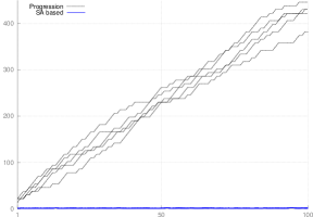
(a) $\mathsf{G}(\forall x:p.\ r(x)\Rightarrow\mathsf{G}\forall y:q.s(y))$

(b) $\mathsf{G}(\forall x:p.\ r(x)\Rightarrow\mathsf{X}s(x))$

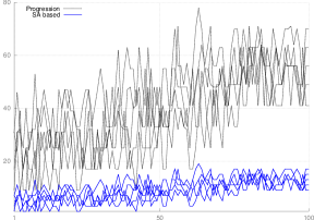
(c) $\mathsf{G}(\forall x:p.\ r(x)\mathsf{U}\mathsf{X}s(x))$

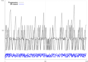
(d) $\mathsf{G}(\forall x:p.\ r(x)\mathsf{U}_{w}\forall y:q.\ \mathsf{X}s(y))$

Figure 1: Automata- (blue lines) vs. progression-based (black dashed lines) $\operatorname{LTL}^{\hbox{\tiny{$\operatorname{FO}$}}}$-monitoring.

6 Related work

This is by no means the first work to discuss monitoring of first-order specifications. Mainly motivated by checking temporal triggers and temporal constraints, the monitoring problem for different types of first-order logic has been widely studied in the database community, for example. In that context, Chomicki [7] presents a method to check for violations of temporal constraints, specified using (metric) past temporal operators. The logic in [7] differs from $\operatorname{LTL}^{\hbox{\tiny{$\operatorname{FO}$}}}$ in that it allows natural first-order quantification over a single countable and constant domain, whereas quantified variables in $\operatorname{LTL}^{\hbox{\tiny{$\operatorname{FO}$}}}$ range over elements that occur at the current position of the trace (see also [13, 4]). Presumably, to achieve the same effect, [7] demands that policies are what is called “domain independent”, so that statements are only ever made wrt. known objects. As such, domain independence is a property of the policy and shown to be undecidable. In contrast, one could say that $\operatorname{LTL}^{\hbox{\tiny{$\operatorname{FO}$}}}$ has a similar notion of domain independence already built-in, because of its quantifier. Like $\operatorname{LTL}^{\hbox{\tiny{$\operatorname{FO}$}}}$, the logic in [7] is also undecidable; no function symbols are allowed and relations are required to be finite. However, despite the fact that the prefix problem is not phrased as a decision problem, its basic idea is already denoted by Chomicki under the notion of a potential constraint satisfaction problem. In particular, he shows that the set of prefixes of models for a given formula is not recursively enumerable. On the other hand, the monitor in [7] does not tackle this problem and instead solves what we have introduced as the word problem, which, unlike the prefix problem, is decidable.

Basin et al. [3] extend Chomicki’s monitor towards bounded future operators using the same logic. Furthermore, they allow infinite relations as long as these are representable by automatic structures, i.e., automata models. In this way, they show that the restriction on formulae to be domain independent is no longer necessary. $\operatorname{LTL}^{\hbox{\tiny{$\operatorname{FO}$}}}$, in comparison, is more general, in that it allows computable relations and functions.

The already cited work of Hallé and Villemaire [13] describes a monitor for a logic with quantification identical to ours, but without function symbols and only equality instead of arbitrary computable relations. Furthermore, the size of the individual worlds is a priori bounded by a fixed value. Additionally, their monitor is fully generated “on the fly” by using syntax-based decomposition rules, similar to formula progression. In our approach, however, it is possible to pre-compute the individual BAs for the respective subformulae of a policy/levels of the SA, and thereby bound the complexity of that part of our monitor at runtime by a constant factor.

Sistla and Wolfson [19] also discuss a monitor for database triggers whose conditions are specified in a logic, which uses an assignment quantifier that binds a single value or a relation instance to a global, rigid variable. Their monitor is represented by a graph structure, which is extended by one level for each updated database state, and as such proportional in size to the number of updates.

7 Conclusions

To the best of our knowledge, our monitoring algorithm is the first to devise anticipatory monitors, i.e., address the prefix problem instead of a (variant of the) word problem, for policies given in an undecidable first-order temporal logic. Moreover, unlike other approaches, such as [19, 13] and even [5], we are able to precompute most of the state space required at runtime (i.e., replace step T1 in Algorithm T with a look-up in a precomputed table of SAs and merely use a new valuation), as the different levels of our SAs correspond to more or less standard BAs that can be generated before monitoring commences. Moreover as required, our monitor is monotonic and in principle trace-length independent. The latter, however, deserves closer examination. Consider the formula given in Fig. 1 (c): it basically forces the monitor to memorise all occurrences of $p$ in every event and keep them until $s(x)$ holds, respectively. If $s(x)$ never holds (or not for a very long time), the space consumption of the monitor is bound to grow. Hence, unlike in standard $\operatorname{LTL}$, trace-length dependence is not merely a property of the monitor, but also of the specification. We have not yet investigated whether trace-length dependence is decidable and if so, at what cost. However, if the formula is not trace-length dependent, then our monitor is trace-length independent, as desired. Given a $\varphi\in\operatorname{LTL}^{\hbox{\tiny{$\operatorname{FO}$}}}$ of which we know that it is trace-length independent in principle, our monitor’s size at runtime at any given time is bounded by $O(|\sigma|^{\operatorname{depth}(\varphi)}\cdot 2^{|cl(\varphi)|})$, where $\sigma$ is the current input to the monitor: Throughout the $\operatorname{depth}(\varphi)$ levels of the monitor, there are a total of $O(|\sigma|^{\operatorname{depth}(\varphi)})$ “submonitors”, which are of size $O(2^{|cl(\varphi)|})$, respectively. In contrast, the size of a progression-based monitor, even for obviously trace-length independent formulae, such as given in Fig. 1 (a) is, in the worst case, proportional to the length of the trace so far.

In Table 1 we have summarised the main results of §2–§4, highlighting again the differences of $\operatorname{LTL}$ compared to $\operatorname{LTL}^{\hbox{\tiny{$\operatorname{FO}$}}}$. Note that as far as trace-length dependence goes, for $\operatorname{LTL}$ it is always possible to devise a trace-length independent monitor (cf. [6]).

Table 1: Overview of complexity results.

	Satisfiability	Word problem	Model checking	Prefix problem
$\operatorname{LTL}$	PSpace-complete	$<$ Bilinear-time	PSpace-complete	PSpace-complete
$\operatorname{LTL}^{\hbox{\tiny{$\operatorname{FO}$}}}$	Undecidable	PSpace-complete	ExpSpace-membership, PSpace-hard	Undecidable

Acknowledgements.

Our thanks go to Patrik Haslum, Michael Norrish and Peter Baumgartner for helpful comments on earlier drafts of this paper.

Appendix 0.A Detailed proofs

Lemma 1. Let $\varphi$ be a sentence in first-order logic, then we can construct a corresponding $\psi\in\operatorname{LTL}^{\hbox{\tiny{$\operatorname{FO}$}}}$ s.t. $\varphi$ has a finite model iff $\psi$ is satisfiable.

Proof

We construct $\psi$ as follows. We first introduce a new unary $\mathbf{U}$-operator $d$ whose arity is $\tau$ and that does not appear in $\varphi$. We then replace every subformula in $\varphi$, which is of the form $\forall x.\ \theta$, with $\forall x:d.\ \theta$ (resp. for $\exists x.\ \theta$). Next, we encode some restrictions on the interpretation of function and predicate symbols:

• For each constant symbol $c$ in $\varphi$, we conjoin the obtained $\psi$ with $d(c)$.

• For each function symbol $f$ in $\varphi$ of arity $n$, we conjoin the obtained $\psi$ with $\forall x_{1}:d.\ \ldots\forall x_{n}:d.\ d(f(x_{1},\ldots,x_{n}))$.

• For each predicate symbol $p$ in $\varphi$ of arity $n$, we conjoin the obtained $\psi$ with $\forall(x_{1},\ldots,x_{n}):p.\ d(x_{1})\wedge\ldots\wedge d(x_{n})$.

• We conjoin $\exists x:d.\ d(x)$ to the obtained $\psi$ to ensure that the domain is not empty.

Finally, we fix the arities of symbols in $\psi$ appropriately to one of the following $\tau$, $\tau\times\ldots\times\tau$, $\tau\times\ldots\times\tau\rightarrow\tau$.

Obviously, the formula $\psi$, constructed by the procedure above, is a syntactically correct $\operatorname{LTL}^{\hbox{\tiny{$\operatorname{FO}$}}}$ formula. Now, if $\psi$ is satisfiable by some $(\mathfrak{A}^{\prime},\sigma)$, where $\mathfrak{A}^{\prime}=(|\mathfrak{A}^{\prime}|,I^{\prime})$ and $\sigma\in(\mathfrak{A}^{\prime})$-$\operatorname{Ev}$, it is easy to construct a finite model $\mathfrak{A}=(|\mathfrak{A}|,I)$ s.t. $\mathfrak{A}\models\varphi$ holds in the classical sense of first-order logic: set $|\mathfrak{A}|=d^{I^{\prime}}$, $c^{I}=c^{I^{\prime}}$, $f^{I}=f^{I^{\prime}}|_{d^{I^{\prime}}\times\ldots\times d^{I^{\prime}}}$, $p^{I}=p^{I^{\prime}}$, respectively. By an inductive argument one can show that the $\operatorname{LTL}^{\hbox{\tiny{$\operatorname{FO}$}}}$semantics is preserved. The other direction, if $\varphi$ is finitely satisfiable, is trivial: set $|\mathfrak{A}^{\prime}|=\tau^{I^{\prime}}=|\mathfrak{A}|$, $c^{I^{\prime}}=c^{I}$, $f^{I^{\prime}}=f^{I}$, respectively, and $\sigma=\{(p,\vec{e})\mid\vec{e}\in p^{I}\}\cup\{(d,e)\mid e\in|\mathfrak{A}|\}$. ∎

Theorem 4.2. The word problem for $\operatorname{LTL}^{\hbox{\tiny{$\operatorname{FO}$}}}$ is PSpace-complete.

Proof

To evaluate a formula $\varphi\in\operatorname{LTL}^{\hbox{\tiny{$\operatorname{FO}$}}}$ over some linear Kripke structure, $\mathcal{K}$, we can basically use the inductive definition of the semantics of $\operatorname{LTL}^{\hbox{\tiny{$\operatorname{FO}$}}}$: If used as a function, starting in the initial state of $\mathcal{K}$, $s_{0}$, it evaluates $\varphi$ in a depth-first manner with the maximal depth bounded by $|\varphi|$.

To show hardness, we reduce the following problem, which is known to be PSpace-complete: Let $F=Q_{1}x_{1}.\ Q_{2}x_{2}.\ \ldots Q_{n}x_{n}.\ E(x_{1},x_{2},\ldots,x_{n})$, where $Q\in\{\forall,\exists\}$ and $E$ is a Boolean expression over variables $x_{1},x_{2},\ldots,x_{n}$. Does $F$ evaluate to $\top$ (cf. [11])? The reduction of this problem proceeds as follows. We first construct a formula $\varphi\in\operatorname{LTL}^{\hbox{\tiny{$\operatorname{FO}$}}}$ in prenex normal form,

$$\varphi=Q_{1}x_{1}:d.\ Q_{2}x_{2}:d.\ \ldots Q_{n}x_{n}:d.\ E(p_{x_{1}}(x_{1}),p_{x_{2}}(x_{2}),\ldots,p_{x_{n}}(x_{n})).$$

Then, using an $\mathbf{U}$-operator $p_{x_{i}}$ for every variable $x_{i}$, we construct a singleton Kripke structure, $\mathcal{K}$, s.t. $\lambda(s_{0})=(\mathfrak{A},\{(d,0),(d,1),(p_{x_{1}},1),(p_{x_{2}},1),\ldots,(p_{x_{n}},1)\}),$ where $|\mathfrak{A}|=\{0,1\}$ and $I$ defined accordingly. It can easily be seen that $F$ evaluates to $\top$ iff $\mathcal{K}$ is a model for $\varphi$. Moreover, this construction can be obtained in no more than a polynomial number of steps wrt. the size of the input. ∎

Theorem 4.3. The model checking problem for $\operatorname{LTL}^{\hbox{\tiny{$\operatorname{FO}$}}}$ is in ExpSpace.

Proof

For a given $\varphi\in\operatorname{LTL}^{\hbox{\tiny{$\operatorname{FO}$}}}$ and $(\mathfrak{A})$-Kripke structure $\mathcal{K}$ defined as usual, where $\mathfrak{A}=(|\mathfrak{A}|,I)$, we construct a propositional Kripke structure $\mathcal{K}^{\prime}$ and $\varphi^{\prime}\in\operatorname{LTL}$, s.t. $\mathcal{L}(\mathcal{K})\subseteq\mathcal{L}(\varphi)$ iff $\mathcal{L}(\mathcal{K}^{\prime})\subseteq\mathcal{L}(\varphi^{\prime})$ holds. Assuming variable names in $\varphi$ have been adjusted so that each has a unique name, the construction of $\varphi^{\prime}$ proceeds as follows.

Wlog. we can assume $|\mathfrak{A}|$ to be a finite set $\{d_{0},\ldots,d_{n}\}$. We first set $\varphi^{\prime}$ to $\varphi$ and extend the corresponding $\Gamma$ by the constant symbols $c_{d_{0}},\ldots,c_{d_{n}}$, s.t. $c_{d_{i}}^{I}=d_{i}$, respectively; that is, we add the respective interpretations of each $c_{d_{i}}$ to $I$. This step obviously does not require more than polynomial space. We then replace all subformulae in $\varphi^{\prime}$ of the form $\nu=Q\operatorname{\vec{x}}:p.\ \psi(\operatorname{\vec{x}})$ exhaustively with the following constructed $\psi^{\prime}$:

• Set $\psi^{\prime}=\top$.

• For each state $s\in S$ do the following:

  • Let $T=\{\operatorname{\vec{d}}\mid\lambda(s)=(\mathfrak{A}^{\prime},\sigma),\mathfrak{A}^{\prime}\sim\mathfrak{A}\hbox{ and }(p,\operatorname{\vec{d}})\in\sigma\}$.

  • If $Q=\forall$, then

    $$\psi^{\prime}=\psi^{\prime}\wedge(\tilde{s}\Rightarrow\bigwedge_{\operatorname{\vec{d}}\in T}\psi(\operatorname{\vec{x}})[\operatorname{\vec{c}}/\operatorname{\vec{x}}]),\hbox{where }\operatorname{\vec{c}}\hbox{ is s.t.\ }\operatorname{\vec{c}}^{I}=\operatorname{\vec{d}},$$

    otherwise

    $$\psi^{\prime}=\psi^{\prime}\wedge(\tilde{s}\Rightarrow\bigvee_{\operatorname{\vec{d}}\in T}\psi(\operatorname{\vec{x}})[\operatorname{\vec{c}}/\operatorname{\vec{x}}]),\hbox{where }\operatorname{\vec{c}}\hbox{ is s.t.\ }\operatorname{\vec{c}}^{I}=\operatorname{\vec{d}},$$

    where $\tilde{s}$ is a fresh, unique predicate symbol meant to represent state $s$.

Then, for all subformulae in $\varphi^{\prime}$ of the form $\tilde{s}\Rightarrow\psi$ we do the following:

• For each $r(\operatorname{\vec{t}})$ occurring in $\psi$, where $r\in\mathbf{R}$ and $\operatorname{\vec{t}}$ are terms, let $\operatorname{\vec{d}}=\operatorname{\vec{t}}^{I}$, and replace $r(\operatorname{\vec{t}})$ by a fresh, unique predicate symbol $r_{\operatorname{\vec{d}}}$.

It is easy to see that, indeed, $\varphi^{\prime}$ is a syntactically correct standard LTL formula, where all quantifiers have been eliminated. In terms of space complexity, note that in the first loop, we replace each quantified formula by an expression at least $|\mathcal{K}|$ times longer than the original quantified formula. In the worst case, the final formula’s length will be exponential in the number of quantifiers.

We now define the propositional Kripke structure $\mathcal{K}^{\prime}=(S^{\prime},s^{\prime}_{0},\lambda^{\prime},\rightarrow^{\prime})$ as follows. Let $S^{\prime}=S$, $s^{\prime}_{0}=s_{0}$, and $\rightarrow^{\prime}=\rightarrow$. In what follows, let $s$ be a state and $\lambda(s)=((|\mathfrak{A}|,I),\sigma)$. (Note, this is the labelling function of $\mathcal{K}$.) The alphabet of $\mathcal{K}^{\prime}$ is given by $2^{\operatorname{AP}}$, where $\operatorname{AP}=\{r_{\operatorname{\vec{d}}}\mid r\in\mathbf{R}\hbox{ and }\operatorname{\vec{d}}\in|\mathfrak{A}|\}\cup\{\tilde{s}\mid s\in S\}$. Finally, we define the labelling function of $\mathcal{K}^{\prime}$ as $\lambda^{\prime}(s)=\{\tilde{s}\}\cup\{r_{\operatorname{\vec{d}}}\mid r\in\mathbf{R}\hbox{ and }r^{I}(\operatorname{\vec{d}})\hbox{ is true}\}.$ It is easy to see that, indeed, $\mathcal{K}^{\prime}$ preserves all the runs possible through $\mathcal{K}$.

One can show by an easy induction on the structure of $\varphi^{\prime}$ that, indeed, $\mathcal{L}(\mathcal{K})\subseteq\mathcal{L}(\varphi)$ iff $\mathcal{L}(\mathcal{K}^{\prime})\subseteq\mathcal{L}(\varphi^{\prime})$ holds. ∎

Lemma 2. Let $\mathfrak{A}$ be a first-order structure and $\varphi\in\operatorname{LTL}^{\hbox{\tiny{$\operatorname{FO}$}}}$, then $\mathcal{L}(\varphi)_{\mathfrak{A}}=\{(\overline{\mathfrak{A}},w)\mid\overline{\mathfrak{A}}\sim\mathfrak{A},w\in(2^{\operatorname{Ev}})^{\omega},\hbox{ and }(\overline{\mathfrak{A}},w)\models\varphi\}$. Testing if $\mathcal{L}(\varphi)_{\mathfrak{A}}\neq\emptyset$ is generally undecidable.

Proof

Let $K=(x_{1},y_{1}),\ldots,(x_{k},y_{k})$ be an instance of Post’s Correspondence Problem over $\Sigma=\{0,1\}$, where $x_{i},y_{i}\in\Sigma^{+}$, which is known to be undecidable in this form. Let us now define a formula $\varphi_{K}=\exists\gamma:z.\ pcp(\gamma)$, a structure $\mathfrak{A}=(\Sigma^{+},I)$, s.t. $pcp^{I}(u)\Leftrightarrow u=x_{i_{1}}\ldots x_{i_{n}}=y_{i_{1}}\ldots y_{i_{n}}$, where $u\in\Sigma^{+}$ and $pcp$ is of corresponding arity. Obviously, $pcp^{I}(u)$ can be computed in finite time for any given $u$. Let us now show that $\mathcal{L}(\varphi_{K})_{\mathfrak{A}}\neq\emptyset$ iff $K$ has a solution.

($\Rightarrow$:) Because $\mathcal{L}(\varphi_{K})_{\mathfrak{A}}\neq\emptyset$, let’s assume there is a word $u\in\Sigma^{+}$ st. $(z,u)\in\sigma$ and  $(\mathfrak{A},\sigma)\in\mathcal{L}(\varphi_{K})_{\mathfrak{A}}$. By the choice of $pcp^{I}$, there exists a sequence of indices, $i_{1},\ldots,i_{n}$, st. $u=x_{i_{1}}\ldots x_{i_{n}}=y_{i_{1}}\ldots y_{i_{n}}$, i.e., $K$ has a solution.

($\Leftarrow$:) Let’s assume $K$ has a solution, i.e., there exists a word $u\in\Sigma^{+}$ and a sequence of indices, $i_{1},\ldots,i_{n}$, st. $u=x_{i_{1}}\ldots x_{i_{n}}=y_{i_{1}}\ldots y_{i_{n}}$. We now have to show that $\mathcal{L}(\varphi_{K})_{\mathfrak{A}}\neq\emptyset$. For this purpose, set $\sigma=\{(z,u)\}$, then $(\mathfrak{A},\sigma)\in\mathcal{L}(\varphi_{K})_{\mathfrak{A}}$ and, consequently, $\mathcal{L}(\varphi_{K})_{\mathfrak{A}}\neq\emptyset$. ∎

Theorem 4.4. The prefix problem for $\operatorname{LTL}^{\hbox{\tiny{$\operatorname{FO}$}}}$ is undecidable.

Proof

By way of a similar reduction used in Theorem 2.1 already, i.e., for any $\varphi$, $\mathfrak{A}$, and $\sigma\in\operatorname{Ev}$ we have that $(\mathfrak{A},\sigma)\in\operatorname{bad}(\mathsf{X}\varphi)$ iff $\mathcal{L}(\varphi)_{\mathfrak{A}}=\emptyset$. The $\Leftarrow$-direction is obvious. For the other direction:

$$\begin{array}[]{ll}&(\mathfrak{A},\sigma)\in\operatorname{bad}(\mathsf{X}\varphi)\\ \Rightarrow&\hbox{for all }\overline{\mathfrak{A}}\sim\mathfrak{A}\hbox{ and }w\in\operatorname{Ev}^{\omega},\hbox{ we have that }(\mathfrak{A}\overline{\mathfrak{A}},\sigma w)\not\models\mathsf{X}\varphi\\ \Rightarrow&\hbox{for all }\overline{\mathfrak{A}}\sim\mathfrak{A}\hbox{ and }w\in\operatorname{Ev}^{\omega},\hbox{ we have that }(\overline{\mathfrak{A}},w)\not\models\varphi\\ \Rightarrow&\mathcal{L}(\varphi)_{\mathfrak{A}}=\emptyset\hbox{ (which is generally undecidable by Lemma~{}\ref{lem:fo:restricted})}.\end{array}$$

∎

Lemma 3. Let $\varphi\in\operatorname{LTL}^{\hbox{\tiny{$\operatorname{FO}$}}}$ (not necessarily a sentence) and $v$ be a valuation. For each accepting run $\rho$ in $\mathcal{A}_{\varphi,v}$ over input $(\overline{\mathfrak{A}},w)$, $\psi\in\operatorname{cl}(\varphi)$, and $i\geq 0$, we have that $\psi\in\rho(i)$ iff $(\overline{\mathfrak{A}},w,v,i)\models\psi$.

Proof

We proceed by a nested induction on $\operatorname{depth}(\varphi)$ and the structure of $\psi\in\operatorname{cl}(\varphi)$. For the base case let $\operatorname{depth}(\varphi)=0$: We fix $\rho$ to be an accepting run in $\mathcal{A}_{\varphi,v}$ over $(\overline{\mathfrak{A}},w)$, and proceed by induction over those formulae $\psi\in\operatorname{cl}(\varphi)$ which are of depth zero (i.e., without quantifiers) since $\operatorname{depth}(\varphi)=0$. Therefore, this case basically resembles the correctness argument of Büchi automata for propositional LTL (cf. [2, §5]). For an arbitrary $i\geq 0$, we have

• $\psi=r(\operatorname{\vec{t}})$:

  $$\begin{array}[]{lcl}r(\operatorname{\vec{t}})\in\rho(i)&\Leftrightarrow&\operatorname{\vec{t}}^{I_{i}}\in r^{I_{i}}(\hbox{by the definition of }\delta_{\rightarrow}),\\ &&\hbox{where, as before, for any variable }x\hbox{ in }\operatorname{\vec{t}},\hbox{ by }x^{I_{i}}\hbox{ we mean }v(x)\\ &\Leftrightarrow&(\overline{\mathfrak{A}},w,v,i)\models r(\operatorname{\vec{t}})\ (\hbox{by the semantics of }\operatorname{LTL}^{\hbox{\tiny{$\operatorname{FO}$}}})\end{array}$$

• $\psi=p(\operatorname{\vec{t}})$: analogous to the above.

• $\psi=\neg\psi^{\prime}$:

  $$\begin{array}[]{ll}\neg\psi^{\prime}\in\rho(i)&\Leftrightarrow\psi^{\prime}\not\in\rho(i)\ (\hbox{by the completeness assumption of all }q\in Q)\\ &\Leftrightarrow(\overline{\mathfrak{A}},w,v,i)\not\models\psi^{\prime}\ (\hbox{by induction hypothesis})\\ &\Leftrightarrow(\overline{\mathfrak{A}},w,v,i)\models\neg\psi^{\prime}\ (\hbox{by the semantics of }\operatorname{LTL}^{\hbox{\tiny{$\operatorname{FO}$}}})\end{array}$$

• $\psi=\psi_{1}\wedge\psi_{2}$:

  $$\begin{array}[]{ll}\psi_{1}\wedge\psi_{2}\in\rho(i)&\Leftrightarrow\{\psi_{1},\psi_{2}\}\subseteq\rho(i)\ (\hbox{by the completeness assumption of all }q\in Q)\\ &\Leftrightarrow(\overline{\mathfrak{A}},w,v,i)\models\psi^{\prime}_{1}\hbox{ and }(\overline{\mathfrak{A}},w,v,i)\models\psi_{2}\ (\hbox{by induction hypothesis})\\ &\Leftrightarrow(\overline{\mathfrak{A}},w,v,i)\models\psi_{1}\wedge\psi_{2}\ (\hbox{by the semantics of }\operatorname{LTL}^{\hbox{\tiny{$\operatorname{FO}$}}})\end{array}$$

• $\psi=\mathsf{X}\psi^{\prime}$:

  $$\begin{array}[]{ll}\mathsf{X}\psi^{\prime}\in\rho(i)&\Leftrightarrow\psi^{\prime}\in\rho(i+1)\ (\hbox{by the definition of }\delta_{\rightarrow})\\ &\Leftrightarrow(\overline{\mathfrak{A}},w,v,i+1)\models\psi^{\prime}\ (\hbox{by induction hypothesis})\\ &\Leftrightarrow(\overline{\mathfrak{A}},w,v,i)\models\mathsf{X}\psi^{\prime}\ (\hbox{by the semantics of }\operatorname{LTL}^{\hbox{\tiny{$\operatorname{FO}$}}})\end{array}$$

• $\psi=\psi_{1}\mathsf{U}\psi_{2}$: we first show the $\Rightarrow$-direction. For this, let us first show that there is a $j\geq i$, such that $(\overline{\mathfrak{A}},w,v,j)\models\psi_{2}$ holds. For suppose not, then for all $j\geq i$, we have that $(\overline{\mathfrak{A}},w,v,j)\not\models\psi_{2}$ and, consequently, by induction hypothesis $\psi_{2}\not\in\rho(j)$. By definition of $\delta_{\rightarrow}$, since $\psi_{1}\mathsf{U}\psi_{2}\in\rho(i)$ and there isn’t a $j$ s.t. $\psi_{2}\in\rho(j)$, we have that $\psi_{1}\mathsf{U}\psi_{2}\in\rho(j)$ for all $j\geq 0$. On the other hand, $\rho$ is accepting in $\mathcal{A}_{\varphi}$, thus there exist infinitely many $j\geq i$, s.t. $\psi_{1}\mathsf{U}\psi_{2}\not\in\rho(j)$ or $\psi_{2}\in\rho(j)$ by the definition of the generalised Büchi acceptance condition $\mathcal{F}$, which is a contradiction. Let us, in what follows, fix the smallest such $j$. We still need to show that for all $i\leq k\leq j$, $(\overline{\mathfrak{A}},w,v,k)\models\psi_{1}$ holds. As $j$ is the smallest such $j$, where $\psi_{2}\in\rho(j)$ it follows that $\psi_{2}\not\in\rho(k)$ for any such $k$. As $\psi_{1}\mathsf{U}\psi_{2}\in\rho(i)$, it follows by definition of $\delta_{\rightarrow}$ that $\psi_{1}\in\rho(i)$ and $\psi_{1}\mathsf{U}\psi_{2}\in\rho(i+1)$. We can then inductively apply this argument to all $i\leq k<j$, such that $\psi_{1}\in\rho(k)$ and $\psi_{1}\mathsf{U}\psi_{2}\in\rho(k+1)$ hold. The statement then follows from the induction hypothesis.
  

  Let us now focus on the $\Leftarrow$-direction, i.e., suppose $(\overline{\mathfrak{A}},w,v,i)\models\psi_{1}\mathsf{U}\psi_{2}$ implies that $\psi_{1}\mathsf{U}\psi_{2}\in\rho(i)$. By assumption, there is a $j\geq i$, such that $(\overline{\mathfrak{A}},w,v,j)\models\psi_{2}$ and for all $i\leq k<j$, we have that $(\overline{\mathfrak{A}},w,v,k)\models\psi_{1}$. Therefore, by induction hypothesis, $\psi_{2}\in\rho(j)$ and $\psi_{1}\in\rho(k)$ for all such $k$. Then, by the completeness assumption of all $q\in Q$, we also get $\psi_{1}\mathsf{U}\psi_{2}\in p_{j}$, and if $j=i$, we are done. Otherwise with an inductive argument similar to the previous case on $k=j-1$, $k=j-2$, …, $k=i$, we can infer that $\psi_{1}\mathsf{U}\psi_{2}\in\rho(k)$.

Let $\operatorname{depth}(\varphi)=n>0$, i.e., we suppose that our claim holds for all formulae with quantifier depth less than $n$. We continue our proof by structural induction, where the quantifier free cases are almost exactly as above. Therefore, we focus only on the following case.

• $\psi=\forall\vec{x}:p.\ \psi^{\prime}$: for this case, as before with the $\mathsf{U}$-operator, we will first show the $\Rightarrow$-direction, i.e., for all $i\geq 0$ we have $\forall\vec{x}:p.\ \psi^{\prime}\in\rho(i)$ implies $(\overline{\mathfrak{A}},w,v,i)\models\forall\vec{x}:p.\ \psi^{\prime}$. By the semantics of $\operatorname{LTL}^{\hbox{\tiny{$\operatorname{FO}$}}}$, the latter is equivalent to for all $(p,\operatorname{\vec{d}})\in w_{i}$, $(\overline{\mathfrak{A}},w,v\cup\{\operatorname{\vec{x}}\mapsto\operatorname{\vec{d}}\},i)\models\psi^{\prime}$. If there is no $(p,\operatorname{\vec{d}})\in w_{i}$ the statement is vacuously true. Otherwise, there are some actions $(p,\operatorname{\vec{d}})\in w_{i}$ and

  $$\delta_{\downarrow}(\rho(i),(\mathfrak{A}_{i},w_{i}))=B\land\bigwedge_{(p,\operatorname{\vec{d}})\in w_{i}}\mathcal{A}_{\psi^{\prime},v\cup\{\operatorname{\vec{x}}\mapsto\operatorname{\vec{d}}\}},$$

  where $B$ is a Boolean combination of SAs corresponding to the remaining elements in $\rho(i)$. As $\rho$ is accepting in $\mathcal{A}_{\varphi,v}$, there exists a $Y_{i}$ satisfying $\delta_{\downarrow}(\rho(i),(\mathfrak{A}_{i},w_{i}))$, s.t. all $\mathcal{A}\in Y_{i}$ have an accepting run on input $(\overline{\mathfrak{A}}^{i},w^{i})$. It follows that $Y_{i}$ contains an automaton $\mathcal{A}_{\psi^{\prime},v\cup\{\operatorname{\vec{x}}\mapsto\operatorname{\vec{d}}\}}$ for each action $(p,\operatorname{\vec{d}})\in w_{i}$ that has an accepting run $\rho^{\prime}$. As the respective levels of these automata is $n-1$, we can use the induction hypothesis and note that the following holds true for each of the $\mathcal{A}_{\psi^{\prime},v\cup\{\operatorname{\vec{x}}\mapsto\operatorname{\vec{d}}\}}\in Y_{i}$:

  $$\hbox{for all: }\nu\in\operatorname{cl}(\psi^{\prime})\hbox{ and }l\geq 0,\nu\in\rho^{\prime}(l)\hbox{ iff }(\overline{\mathfrak{A}},w,v\cup\{\operatorname{\vec{x}}\mapsto\operatorname{\vec{d}}\},i+l)\models\nu,$$

  We can now set $\nu=\psi^{\prime}$, respectively, and $l=0$, from which it follows that $\psi^{\prime}\in\rho^{\prime}(0)$ iff $(\overline{\mathfrak{A}},w,v\cup\{\operatorname{\vec{x}}\mapsto\operatorname{\vec{d}}\},i)\models\psi^{\prime}$, respectively. As by construction of an SA the initial states of runs contain the formula which the SA represents, we have $\psi^{\prime}\in\rho^{\prime}(0)$ and hence $(\overline{\mathfrak{A}},w,v\cup\{\operatorname{\vec{x}}\mapsto\operatorname{\vec{d}}\},i)\models\psi^{\prime}$, respectively. As this holds for all $\mathcal{A}_{\psi^{\prime},v\cup\{\operatorname{\vec{x}}\mapsto\operatorname{\vec{d}}\}}$, where $(p,\operatorname{\vec{d}})\in w_{i}$, it follows by semantics of $\operatorname{LTL}^{\hbox{\tiny{$\operatorname{FO}$}}}$ that $(\overline{\mathfrak{A}},w,v,i)\models\forall\vec{x}:p.\ \psi^{\prime}$.

  Let us now consider the $\Leftarrow$-direction, i.e., $(\overline{\mathfrak{A}},w,v,i)\models\forall\vec{x}:p.\ \psi^{\prime}$ implies $\forall\vec{x}:p.\ \psi^{\prime}\in\rho(i)$, which we show by contradiction. Suppose $\forall\vec{x}:p.\ \psi^{\prime}\not\in\rho(i)$, which implies by the completeness assumption of all $q\in Q$ that $\neg\forall\vec{x}:p.\ \psi^{\prime}\in\rho(i)$ holds. If there is no $(p,\operatorname{\vec{d}})\in w_{i}$, then $\delta_{\downarrow}(\rho(i),(\mathfrak{A}_{i},w_{i}))$ is equivalent to $\bot$ and $\rho$ could not be accepting. Therefore there must be some $(p,\operatorname{\vec{d}})\in w_{i}$, s.t.

  $$\delta_{\downarrow}(\rho(i),(\mathfrak{A}_{i},w_{i}))=B\land\bigvee_{(p,\operatorname{\vec{d}})\in w_{i}}\mathcal{A}_{\neg\psi^{\prime},v\cup\{\operatorname{\vec{x}}\mapsto\operatorname{\vec{d}}\}},$$

  where $B$ is a Boolean combination of SAs corresponding to the remaining elements in $\rho(i)$. Because $\rho$ is accepting in $\mathcal{A}_{\varphi,v}$, there exists a $Y_{i}$, such that $Y_{i}\models\delta_{\downarrow}(\rho(i),(\mathfrak{A}_{i},w_{i}))$, and there is at least one SA, $\mathcal{A}^{\prime}=\mathcal{A}_{\neg\psi^{\prime},v\cup\{\operatorname{\vec{x}}\mapsto\operatorname{\vec{d}}\}}\in Y_{i}$, with corresponding $(p,\operatorname{\vec{d}})\in w_{i}$, s.t. $(\overline{\mathfrak{A}}^{i},w^{i})$ is accepted by $\mathcal{A}^{\prime}$ as input; that is, $\mathcal{A}^{\prime}$ has an accepting run, $\rho^{\prime}$, on said input. As this automaton’s level is $n-1$, we can apply the induction hypothesis and obtain

  $$\hbox{for all: }\nu\in\operatorname{cl}(\neg\psi^{\prime})\hbox{ and }l\geq 0,\nu\in\rho^{\prime}(l)\hbox{ iff }(\overline{\mathfrak{A}},w,v\cup\{\operatorname{\vec{x}}\mapsto\operatorname{\vec{d}}\},i+l)\models\nu.$$

  We can now set $\nu=\neg\psi^{\prime}$ and $l=0$, and since $\nu$ belongs to the initial states in accepting runs, we derive $(\overline{\mathfrak{A}},w,v\cup\{\operatorname{\vec{x}}\mapsto\operatorname{\vec{d}}\},i)\models\neg\psi^{\prime}$, which is a contradiction to our initial hypothesis. ∎

Theorem 5.1. The constructed SA is correct in the sense that for any sentence $\varphi\in\operatorname{LTL}^{\hbox{\tiny{$\operatorname{FO}$}}}$, we have that $\mathcal{L}(\mathcal{A}_{\varphi})=\mathcal{L}(\varphi)$.

Proof

$\subseteq$: Follows from Lemma 3: let $\rho$ be an accepting run over $(\overline{\mathfrak{A}},w)$ in $\mathcal{A}_{\varphi}$. By definition of an (accepting) run, $\varphi\in\rho(0)$, and therefore $(\overline{\mathfrak{A}},w)\in\mathcal{L}(\varphi)$.

$\supseteq$: We show the more general statement: Given a (possibly not closed) formula $\varphi\in\operatorname{LTL}^{\hbox{\tiny{$\operatorname{FO}$}}}$ and valuation $v$. It holds that $\{(\overline{\mathfrak{A}},w)\mid(\overline{\mathfrak{A}},w,v,0)\models\varphi\}\subseteq\mathcal{L}(\mathcal{A}_{\varphi,v})$. We define for all $i\geq 0$ the set $\rho(i)=\{\psi\in\operatorname{cl}(\varphi)\mid(\overline{\mathfrak{A}},w,v,i)\models\psi\}$ for some arbitrary but fixed formula $\varphi\in\operatorname{LTL}^{\hbox{\tiny{$\operatorname{FO}$}}}$ and valuation $v$, and arbitrary but fixed $(\overline{\mathfrak{A}},w)$, where $(\overline{\mathfrak{A}},w,v,0)\models\varphi$. Let us now show that $\rho=\rho(0)\rho(1)\ldots$ is a well-defined run in $\mathcal{A}_{\varphi,v}$ over $(\overline{\mathfrak{A}},w)$: Firstly, from the construction of $Q$, it follows that for all $i$, $\rho(i)\in Q$. Secondly, since $\varphi\in\operatorname{cl}(\varphi)$ and $(\overline{\mathfrak{A}},w,v,0)\models\varphi$, $\rho(0)$ always contains $\varphi$. Thirdly, $\rho(i+1)\in\delta_{\rightarrow}(\rho(i),(\mathfrak{A}_{i},w_{i}))$ holds for all $i$. The latter is the case iff

• for all $\mathsf{X}\psi\in\operatorname{cl}(\varphi)$: $\mathsf{X}\psi\in\rho(i)$ iff $\psi\in\rho(i+1)$, and

• for all $\psi_{1}\mathsf{U}\psi_{2}\in\operatorname{cl}(\varphi)$: $\psi_{1}\mathsf{U}\psi_{2}\in\rho(i)$ iff $\psi_{2}\in\rho(i)$ or ($\psi_{1}\in\rho(1)$ and $\psi_{1}\mathsf{U}\psi_{2}\in\rho(i+1)$).

The first condition can be shown as follows:

$$\begin{array}[]{ll}\mathsf{X}\psi\in\rho(i)&\Leftrightarrow(\overline{\mathfrak{A}},w,v,i)\models\mathsf{X}\psi\ (\hbox{by definition of }\rho(i))\\ &\Leftrightarrow(\overline{\mathfrak{A}},w,v,i+1)\models\psi\ (\hbox{by the semantics of $\operatorname{LTL}^{\hbox{\tiny{$\operatorname{FO}$}}}$})\\ &\Leftrightarrow\psi\in\rho(i+1)\ (\hbox{by the definition of }\rho(i+1)).\end{array}$$

The second can be shown as follows:

$$\begin{array}[]{ll}\psi_{1}\mathsf{U}\psi_{2}\in\rho(i)&\Leftrightarrow(\overline{\mathfrak{A}},w,v,i)\models\psi_{1}\mathsf{U}\psi_{2}\ (\hbox{by definition of }\rho(i))\\ &\Leftrightarrow(\overline{\mathfrak{A}},w,v,i)\models\psi_{2}\vee(\psi_{1}\wedge\mathsf{X}(\psi_{1}\mathsf{U}\psi_{2}))\\ &\Leftrightarrow(\overline{\mathfrak{A}},w,v,i)\models\psi_{2}\hbox{ or }((\overline{\mathfrak{A}},w,v,i)\models\psi_{1}\hbox{ and }(\overline{\mathfrak{A}},w,v,i+1)\models\psi_{1}\mathsf{U}\psi_{2})\\ &\Leftrightarrow\psi_{2}\in\rho(i)\hbox{ or }(\psi_{1}\in\rho(1)\hbox{ and }\psi_{1}\mathsf{U}\psi_{2}\in\rho(i+1))\ (\hbox{by definition of }\rho).\end{array}$$

It remains to show that $\rho$ is also accepting in $\mathcal{A}_{\varphi,v}$. We proceed by induction on $\operatorname{depth}(\varphi)$. In what follows, let $\operatorname{depth}(\varphi)=0$, i.e., we are showing local acceptance only. By the definition of acceptance we must have that for all $\psi_{1}\mathsf{U}\psi_{2}\in\operatorname{cl}(\varphi)$, there exist infinitely many $i\geq 0$, s.t. $\rho(i)\in F_{\psi_{1}\mathsf{U}\psi_{2}}$, where $F_{\psi_{1}\mathsf{U}\psi_{2}}\in\mathcal{F}$. For suppose not, i.e., there are only finitely many such $i$, then there is a $k\geq 0$, s.t. for all $j\geq k$ we have $\rho(j)\not\in F_{\psi_{1}\mathsf{U}\psi_{2}}$ and therefore $\psi_{1}\mathsf{U}\psi_{2}\in\rho(j)$ and $\psi_{2}\not\in\rho(j)$ by definition of $F_{\psi_{1}\mathsf{U}\psi_{2}}$. In particular, from $\psi_{1}\mathsf{U}\psi_{2}\in\rho(k)$ we derive by construction of $\rho(k)$ that there must be some $g\geq k$, s.t. $(\overline{\mathfrak{A}}^{g},w^{g})\in\mathcal{L}(\psi_{2})$ and thus $\psi_{2}\in\rho(k)$ with $g\geq k$. Contradiction.

Let us now assume the statement holds for all formulae with depth strictly less than $n$ and assume $\operatorname{depth}(\varphi)=n$, where $n>0$. We don’t show local acceptance of $\rho$ as it is virtually the same as in the base case, and instead go on to show that for all $i\geq 0$, there is a $Y_{i}$, s.t. $Y_{i}\models\delta_{\downarrow}(\rho(i),(\mathfrak{A}_{i},w_{i}))$ and all $\mathcal{A}\in Y_{i}$ are accepting $(\overline{\mathfrak{A}}^{i},w^{i})$. Let us define the following two sets:

$$Y_{i}^{\forall}=\{\mathcal{A}_{\psi,v\cup\{\operatorname{\vec{x}}\mapsto\operatorname{\vec{d}}\}}\mid\forall\vec{x}:p.\ \psi\in\rho(i)\hbox{ and }(p,\operatorname{\vec{d}})\in w_{i}\}$$

and

$$\begin{array}[]{lll}Y_{i}^{\exists}=\{\mathcal{A}_{\neg\psi,v\cup\{\operatorname{\vec{x}}\mapsto\operatorname{\vec{d}}\}}&\mid&\neg\forall\vec{x}:p.\ \psi\in\rho(i),(p,\operatorname{\vec{d}})\in w_{i},\\ &&\hbox{ and }(\overline{\mathfrak{A}},w,v\cup\{\operatorname{\vec{x}}\mapsto\operatorname{\vec{d}}\},i)\not\models\psi\}.\end{array}$$

Set $Y_{i}=Y_{i}^{\forall}\cup Y_{i}^{\exists}$, which by construction satisfies $\delta_{\downarrow}(\rho(i),(\mathfrak{A}_{i},w_{i}))$. We still need to show that every automaton in this set accepts $(\overline{\mathfrak{A}}^{i},w^{i})$. Now for $\mathcal{A}_{\nu,v\cup\{\operatorname{\vec{x}}\mapsto\operatorname{\vec{d}}\}}\in Y_{i}$ we have either $\nu=\psi$ for some $\forall\vec{x}:p.\ \psi\in\rho(i)$ and $(p,\operatorname{\vec{d}})\in w_{i}$, or $\nu=\neg\psi$ for some $\neg\forall\vec{x}:p.\ \psi\in\rho(i)$ and $(p,\operatorname{\vec{d}})\in w_{i}$ s.t. $(\overline{\mathfrak{A}},w,v\cup\{\operatorname{\vec{x}}\mapsto\operatorname{\vec{d}}\},i)\not\models\psi$ holds. In either case by definition of $\rho(i)$ and semantics of $\operatorname{LTL}^{\hbox{\tiny{$\operatorname{FO}$}}}$, it follows that $(\overline{\mathfrak{A}},w,v\cup\{\operatorname{\vec{x}}\mapsto\operatorname{\vec{d}}\},i)\models\nu$. Since the level of $\mathcal{A}_{\nu,v\cup\{\operatorname{\vec{x}}\mapsto\operatorname{\vec{d}}\}}$ is strictly less than $n$, we can apply the induction hypothesis and construct an accepting run for $(\overline{\mathfrak{A}}^{i},w^{i})$, where $(\overline{\mathfrak{A}},w,v\cup\{\operatorname{\vec{x}}\mapsto\operatorname{\vec{d}}\},i)\models\nu$, in $\mathcal{A}_{\nu,v\cup\{\operatorname{\vec{x}}\mapsto\operatorname{\vec{d}}\}}$. The statement follows. ∎

Theorem 5.2. $M_{\varphi}(\overline{\mathfrak{A}},u)=\top\Rightarrow$ $(\overline{\mathfrak{A}},u)\in\operatorname{good}(\varphi)$ (resp. for $\bot$ and $\operatorname{bad}(\varphi)$).

Proof

We prove the more general statement $M_{\varphi,v}(\overline{\mathfrak{A}},u)=\top\Rightarrow$ $(\overline{\mathfrak{A}},u)\in\operatorname{good}(\varphi,v)$, where $\varphi$ possibly has some free variables and $v$ is a valuation, by a nested induction over $\operatorname{depth}(\varphi)$.

• For the base case let $\operatorname{depth}(\varphi)=0$, where $\varphi$ possibly has free variables, $(\overline{\mathfrak{A}},u)$ be an arbitrary but fixed prefix and $v$ a valuation. Suppose $M_{\varphi,v}(\overline{\mathfrak{A}},u)$ returns $\top$ after processing $(\overline{\mathfrak{A}},u)$, but $(\overline{\mathfrak{A}},u)\not\in\operatorname{good}(\varphi,v)$. By M3. and T10., the buffer of $T_{\lnot\varphi,v}$ is empty, i.e., $B_{\lnot\varphi,v}=\emptyset$. By    T3. and because $\mathcal{A}_{\neg\varphi,v}$ has an accepting run $\rho$ over $(\overline{\mathfrak{A}},u)$ with some suffix, $B_{\neg\varphi,v}$ contains $(\rho(|u|),[\top])$ after processing $(\overline{\mathfrak{A}},u)$. Furthermore, because $\delta_{\downarrow}$ yields $\top$ for any input iff $\operatorname{depth}(\lnot\varphi)=0$, no run in the buffer is ever removed in    T7.. Contradiction.

• Let $depth(\varphi)>0$, $(\overline{\mathfrak{A}},u)$ be an arbitrary but fixed prefix and $v$ a valuation. Under the same assumptions as above, we will reach a contradiction showing that after processing $(\overline{\mathfrak{A}},u)$, there is a sequence of obligations $(\rho(|u|),\allowbreak[obl_{0},\ldots,\allowbreak obl_{n}])$ in buffer $B_{\lnot\varphi,v}$, which corresponds to an accepting run $\rho$ in $\mathcal{A}_{\neg\varphi,v}$ over $(\overline{\mathfrak{A}},u)$ with some suffix $(\overline{\mathfrak{A}}^{\prime},w^{\prime})$. That is, M_φ,v cannot return $\top$, after $B_{\lnot\varphi,v}$ is empty, and $B_{\lnot\varphi,v}$ containing the above mentioned sequence at the same time. By    T3., $B_{\neg\varphi,v}$ contains a sequence $(\rho(|u|),\allowbreak[obl_{0},\ldots,\allowbreak obl_{n}])$ that was incrementally created processing $(\overline{\mathfrak{A}},u)$ wrt. $\delta_{\rightarrow}$, eventually with some obligations removed if they were detected to be met by the input. We now show that this sequence is never removed from the buffer in    T7.. Suppose the run has been removed, then there was an $obl_{j}=\delta_{\downarrow}(\rho(j),(\overline{\mathfrak{A}}_{j},u_{j}))$, that is

  $$\left(\bigwedge_{\forall\operatorname{\vec{x}}:p.\psi\in\rho(j)}\left(\bigwedge_{(p,\operatorname{\vec{d}})\in u_{j}}\mathcal{A}_{\psi,v^{\prime}}\right)\right)\wedge\left(\bigwedge_{\neg\forall\operatorname{\vec{x}}:p.\psi\in\rho(j)}\left(\bigvee_{(p,\operatorname{\vec{d}})\in u_{j}}\mathcal{A}_{\neg\psi,v^{\prime\prime}}\right)\right),$$

  with $v^{\prime}=v\cup\{\operatorname{\vec{x}}\mapsto\operatorname{\vec{d}}\}$ and $v^{\prime\prime}=v\cup\{\operatorname{\vec{x}}\mapsto\operatorname{\vec{d}}\}$, evaluated to $\bot$ after $l$ steps, with $0\leq j\leq l<|u|$. That is, at least one submonitor corresponding to an automaton in the second conjunction has returned $\bot$ (or all submonitors corresponding to automata in a disjunction, for which the following argument would be similar). Wlog. let $\forall\vec{x}:p.\psi\in\rho(j)$, $(p,\operatorname{\vec{d}})\in u_{j}$, and M${}_{\psi,v^{\prime}}(\mathfrak{A}_{j},\ldots,\allowbreak\mathfrak{A}_{l},u_{j},\ldots,u_{l})=\bot$, i.e., M${}_{\psi,v^{\prime}}$ is the submonitor corresponding to $\mathcal{A}_{\psi,v^{\prime}}$. As $level(\psi)<level(\varphi)$, from the induction hypothesis follows that $(\mathfrak{A}_{j},\ldots,\mathfrak{A}_{l},\allowbreak u_{j},\ldots,u_{l})\in bad(\psi,v^{\prime})$, i.e., $(\mathfrak{A}_{j},\ldots,\mathfrak{A}_{l}\overline{\mathfrak{A}}^{\prime\prime},u_{j},\ldots,u_{l}w^{\prime\prime})\models\psi$ with evaluation $v^{\prime}$ for any $(\overline{\mathfrak{A}}^{\prime\prime},w^{\prime\prime})$, and therefore $(\mathfrak{A}_{j},\ldots,\mathfrak{A}_{l}\overline{\mathfrak{A}}^{\prime\prime},u_{j},\ldots,u_{l}w^{\prime\prime})\models\neg\forall x:p.\psi$ under valuation $v$. But as $\rho$ over $(\overline{\mathfrak{A}}\overline{\mathfrak{A}}^{\prime},uw^{\prime})$ is an accepting run in $\mathcal{A}_{\neg\varphi,v}$ and $\forall x:p.\psi\in\rho(j)$, it follows that $(\overline{\mathfrak{A}}^{j}\overline{\mathfrak{A}}^{\prime},u^{j}w^{\prime})\models\forall x:p.\psi$. Now, we choose $(\overline{\mathfrak{A}}^{\prime\prime},w^{\prime\prime})$ to be $(\overline{\mathfrak{A}}_{l+1},\ldots,\overline{\mathfrak{A}}_{|u|}\overline{\mathfrak{A}}^{\prime},\allowbreak u_{l+1},\ldots,u_{|u|}w^{\prime})$. Contradiction.

  As for our second statement above, it can be shown similar as before. ∎

References

• [1] F. Bacchus and F. Kabanza. Planning for temporally extended goals. Annals of Mathematics and Artificial Intelligence, 22:5–27, 1998.
• [2] C. Baier and J.-P. Katoen. Principles of Model Checking. MIT Press, 2008.
• [3] D. Basin, F. Klaedtke, and S. Müller. Policy monitoring in first-order temporal logic. In Proc. 22nd Intl. Conf. on Computer Aided Verification (CAV), volume 6174 of LNCS, pages 1–18. Springer, 2010.
• [4] A. Bauer, R. Gore, and A. Tiu. A first-order policy language for history-based transaction monitoring. In Proc. 6th Intl. Colloq. on Theoretical Aspects of Computing (ICTAC), volume 5684 of LNCS, pages 96–111. Springer, 2009.
• [5] A. Bauer, J.-C. Küster, and G. Vegliach. Runtime verification meets Android security. In Proc. 4th NASA Formal Methods Symp. (NFM), volume 7226 of LNCS, pages 174–180. Springer, 2012.
• [6] A. Bauer, M. Leucker, and C. Schallhart. Runtime verification for LTL and TLTL. ACM Transactions on Software Engineering and Methodology, 20(4):14, 2011.
• [7] J. Chomicki. Efficient checking of temporal integrity constraints using bounded history encoding. ACM Trans. Database Syst., 20(2):149–186, 1995.
• [8] J. Chomicki and D. Niwinski. On the feasibility of checking temporal integrity constraints. J. Comput. Syst. Sci., 51(3):523–535, 1995.
• [9] W. Dong, M. Leucker, and C. Schallhart. Impartial anticipation in runtime-verification. In Proc. 6th Intl. Symposium on Automated Technology for Verification and Analysis (ATVA), volume 5311 of LNCS, pages 386–396. Springer, 2008.
• [10] C. Eisner, D. Fisman, J. Havlicek, Y. Lustig, A. McIsaac, and D. V. Campenhout. Reasoning with temporal logic on truncated paths. In Proc. 15th Intl. Conf. on Computer Aided Verification (CAV), volume 2725 of LNCS, pages 27–39. Springer, 2003.
• [11] M. R. Garey and D. S. Johnson. Computers and Intractability: A Guide to the Theory of NP-Completeness. W. H. Freeman & Co., New York, NY, USA, 1979.
• [12] A. Genon, T. Massart, and C. Meuter. Monitoring distributed controllers: When an efficient LTL algorithm on sequences is needed to model-check traces. In Proc. 14th Intl. Symp. on Formal Methods (FM), volume 4085 of LNCS, pages 557–572. Springer, 2006.
• [13] S. Halle and R. Villemaire. Runtime monitoring of message-based workflows with data. In Proc. 12th IEEE Enterprise Distributed Object Computing Conference (EDOC), pages 63–72. IEEE, 2008.
• [14] K. Havelund and G. Rosu. Efficient monitoring of safety properties. Software Tools for Technology Transfer, 6(2):158–173, 2004.
• [15] L. Kuhtz and B. Finkbeiner. Efficient parallel path checking for linear-time temporal logic with past and bounds. Logical Methods in Computer Science, 8(4), 2012.
• [16] L. Libkin. Elements Of Finite Model Theory. Springer, 2004.
• [17] N. Markey and P. Schnoebelen. Model checking a path. In Proc. 14th Int. Conf. on Concurrency Theory (CONCUR), volume 2761 of LNCS, pages 248–262. Springer, 2003.
• [18] A. P. Sistla and E. M. Clarke. The complexity of propositional linear temporal logics. J. ACM, 32(3):733–749, 1985.
• [19] A. P. Sistla and O. Wolfson. Temporal triggers in active databases. IEEE Trans. Knowl. Data Eng., 7(3):471–486, 1995.