Adaptive Low-rank Constrained Constant Modulus Beamforming Algorithms using Joint Iterative Optimization of Parameters

Abstract

This paper proposes a robust reduced-rank scheme for adaptive beamforming based on joint iterative optimization (JIO) of adaptive filters. The scheme provides an efficient way to deal with filters with large number of elements. It consists of a bank of full-rank adaptive filters that forms a transformation matrix and an adaptive reduced-rank filter that operates at the output of the bank of filters. The transformation matrix projects the received vector onto a low-dimension vector, which is processed by the reduced-rank filter to estimate the desired signal. The expressions of the transformation matrix and the reduced-rank weight vector are derived according to the constrained constant modulus (CCM) criterion. Two novel low-complexity adaptive algorithms are devised for the implementation of the proposed scheme with respect to different constrained conditions. Simulations are performed to show superior performance of the proposed algorithms in comparison with the existing methods.

Index Terms—  Beamforming techniques, antenna array, constrained constant modulus, reduced-rank methods, joint iterative optimization.

1 Introduction

Adaptive beamforming technology is of paramount importance in numerous signal processing applications such as radar, wireless communications, and sonar [2]-[4]. Among various beamforming techniques, the beamformers according to the constrained minimum variance (CMV) criterion [4] are prevalent, which minimize the total output power while maintaining the gain along the direction of the signal of interest (SOI). Another alternative beamformer design is performed according to the constrained constant modulus (CCM) criterion, which is a positive measure [4] of the average amount that the beamformer output deviates from a constant modulus condition. Compared with the CMV, the CCM beamformers exhibit superior performance in many severe scenarios (e.g., steering vector mismatch) since the positive measure provides more information for the parameter estimation.

Many adaptive algorithms have been developed according to the CMV and CCM criteria for implementation. A simple and popular one is stochastic gradient (SG) method [5], [8]. A major drawback of the SG-based methods is that, when the number of elements in the filter is large, they always require a large amount of samples to reach the steady-state. Furthermore, in dynamic scenarios, filters with many elements usually show poor performance in tracking signals embedded in interference and noise. Reduced-rank signal processing was motivated to provide a way out of this dilemma [9], [10]. For the application of beamforming, the reduced-rank technique project the received vector onto a low-dimension subspace and perform the filter optimization within this subspace. One popular reduced-rank scheme is the multistage wiener filter (MSWF), which employs the minimum mean squared error (MMSE) [11], and its extended versions that utilize the CMV and CCM criteria were reported in [12], [13]. Another technique that resembles the MSWF is the auxiliary-vector filtering (AVF) [14], [15]. Despite improved convergence and tracking performance achieved by these methods, their implementations require high computational cost and suffer from numerical problems. A joint iterative optimization (JIO) scheme, which was presented recently in [20], employs the CMV criterion with a low-complexity adaptive implementation to achieve better performance than the existing methods.

Considering the fact that the CCM-based beamformers outperform the CMV ones for constant modulus constellations, we propose a robust reduced-rank scheme according to the CCM criterion for the beamformer design. The proposed reduced-rank scheme consists of a bank of full-rank adaptive filters, which constitutes the transformation matrix, and an adaptive reduced-rank filter that operates at the output of the bank of filters. The transformation matrix projects the full-rank received vector onto a low-dimension, which is then processed by the reduced-rank filter to estimate the desired signal. The transformation matrix and the reduced-rank filter are computed based on the JIO. The proposed scheme provides an iterative exchange of information between the transformation matrix and the reduced-rank filter, which leads to improved convergence and tracking ability and low-complexity cost. We devise two adaptive algorithms for the implementation of the proposed reduced-rank scheme. The first one employs the SG approach to jointly estimate the transformation matrix and the reduced-rank weight vector subject to a constraint on the array response. The second proposed algorithm is extended from the first one and reformulates the transformation matrix subject to an orthogonal constraint. The Gram Schmidt (GS) technique [22] is employed to realize the reformulation. The performance of the second method outperforms the first one. Simulation results are given to demonstrate the preferable performance and stability achieved by the proposed algorithms versus the existing methods in typical scenarios.

2 System Model and Problem Statement

2.1 System Model

Let us suppose that $q$ narrowband signals impinge on an uniform linear array (ULA) of $m$ ($m\geq q$) sensor elements. The sources are assumed to be in the far field with directions of arrival (DOAs) $\theta_{0}$,…,$\theta_{q-1}$. The $i$th received vector $\boldsymbol{x}(i)\in\mathbb{C}^{m\times 1}$ can be modeled as

$$\centering{\boldsymbol{x}}(i)={\boldsymbol{A}}({\boldsymbol{\theta}}){\boldsymbol{s}}(i)+{\boldsymbol{n}}(i),~{}~{}~{}i=1,\ldots,N\@add@centering$$ (1)

where $\boldsymbol{\theta}=[\theta_{0},\ldots,\theta_{q-1}]^{T}\in\mathbb{C}^{q\times 1}$ is the signal DOAs, ${\boldsymbol{A}}({\boldsymbol{\theta}})=[{\boldsymbol{a}}(\theta_{0}),\ldots,{\boldsymbol{a}}(\theta_{q-1})]\in\mathbb{C}^{m\times q}$ comprises the signal direction vectors ${\boldsymbol{a}}(\theta_{k})=[1,e^{-2\pi j\frac{d}{\lambda_{c}}cos{\theta_{k}}},\ldots$, $e^{-2\pi j(m-1)\frac{d}{\lambda_{c}}cos{\theta_{k}}}]^{T}\in\mathbb{C}^{m\times 1}$, $(k=0,\ldots,q-1)$, where $\lambda_{c}$ is the wavelength and $d$ is the inter-element distance of the ULA ($d=\lambda_{c}/2$ in general), and to avoid mathematical ambiguities, the direction vectors $\boldsymbol{a}(\theta_{k})$ are considered to be linearly independents. ${\boldsymbol{s}}(i)\in\mathbb{C}^{q\times 1}$ is the source data, ${\boldsymbol{n}}(i)\in\mathbb{C}^{m\times 1}$ is temporarily white sensor noise, which is assumed to be a zero-mean spatially and Gaussian process, $N$ is the observation size of snapshots, and $(\cdot)^{T}$ stands for transpose. The estimated desired signal is given by

$$\centering y(i)={\boldsymbol{w}}^{H}(i){\boldsymbol{x}}(i)\@add@centering$$ (2)

where ${\boldsymbol{w}}(i)=[w_{1}(i),\ldots,w_{m}(i)]^{T}\in\mathbb{C}^{m\times 1}$ is the complex weight vector, and $(\cdot)^{H}$ stands for Hermitian transpose.

2.2 Problem Statement

Let us consider the full-rank CCM filter for beamforming, which can be computed by minimizing the following cost function

$$J_{\textrm{cm}}\big{(}\boldsymbol{w}(i)\big{)}=\mathbb{E}\big{\{}\big{[}|y(i)|^{2}-1\big{]}^{2}\big{\}},~{}~{}\textrm{subject~{}to}~{}~{}{\boldsymbol{w}}^{H}(i){\boldsymbol{a}}(\theta_{0})=1$$ (3)

where $\theta_{0}$ is the direction of the SOI and $\boldsymbol{a}(\theta_{0})$ denotes the corresponding normalized steering vector. The cost function is the expected deviation of the squared modulus of the array output to a constant subject to the constraint on the array response, which is set to capture the power of the desired signal and ensure the convexity of the cost function. The weight expression obtained from (3) is

$$\boldsymbol{w}(i+1)=\boldsymbol{R}^{-1}(i)\Big{\{}\boldsymbol{p}(i)-\frac{\big{[}\boldsymbol{p}^{H}(i)\boldsymbol{R}^{-1}(i)\boldsymbol{a}(\theta_{0})-1\big{]}\boldsymbol{a}(\theta_{0})}{\boldsymbol{a}^{H}(\theta_{0})\boldsymbol{R}^{-1}(i)\boldsymbol{a}(\theta_{0})}\Big{\}}$$ (4)

where $\boldsymbol{R}(i)=\mathbb{E}[|y(i)|^{2}\boldsymbol{x}(i)\boldsymbol{x}^{H}(i)]$, $\boldsymbol{p}(i)=\mathbb{E}[y^{\ast}(i)\boldsymbol{x}(i)]$, and $(\cdot)^{\ast}$ denotes complex conjugate. Note that (4) is a function of previous values of $\boldsymbol{w}(i)$ (since $y(i)=\boldsymbol{w}^{H}(i)\boldsymbol{x}(i)$) and thus must be initialized to start the iteration. We keep the time index in $\boldsymbol{R}(i)$ and $\boldsymbol{p}(i)$ for the same reason. It is obvious that the calculation of weight vector requires high complexity due to the matrix inversion. The SG type algorithms can be employed to reduce the computational load but still suffer from slow convergence and tracking performance when the dimension $m$ is large. The reduced-rank schemes like MSWF and AVF can be used to improve the performance but still need high computational cost and suffer from numerical problems.

3 Proposed Reduced-rank Scheme and CCM Filters Design

In this section, by proposing a reduced-rank scheme based on the JIO of adaptive filters, we introduce a minimization problem according to the CM criterion subject to different constraints. The reduced-rank CCM filters design is described in details.

3.1 Proposed Reduced-Rank Scheme

Define a transformation matrix $\boldsymbol{T}_{r}(i)=[\boldsymbol{t}_{1}(i),\boldsymbol{t}_{2}(i),\ldots,$ $\boldsymbol{t}_{r}(i)]\in\mathbb{C}^{m\times r}$, which is responsible for the dimensionality reduction, to project the $m\times 1$ received vector $\boldsymbol{x}(i)$ onto a lower dimension, yielding

$$\bar{\boldsymbol{x}}(i)=\boldsymbol{T}_{r}^{H}(i)\boldsymbol{x}(i)$$ (5)

where $\boldsymbol{t}_{l}(i)=[t_{1,l}(i),\ldots,t_{m,l}(i)]^{T}\in\mathbb{C}^{m\times 1},~{}l=1,\ldots,r$, makes up the transformation matrix $\boldsymbol{T}_{r}(i)$, $\bar{\boldsymbol{x}}(i)\in\mathbb{C}^{r\times 1}$ is the projected received vector, and in what follows, all $r$-dimensional quantities are denoted by an over bar. Here, $r<m$ is the rank and, as we will see, impacts the output performance. An adaptive reduced-rank filter represented by $\bar{\boldsymbol{w}}(i)=[\bar{w}_{1}(i),\ldots,\bar{w}_{r}(i)]^{T}\in\mathbb{C}^{r\times 1}$ is followed to get the filter output

$$y(i)=\bar{\boldsymbol{w}}^{H}(i)\boldsymbol{T}_{r}^{H}(i)\boldsymbol{x}(i)$$ (6)

From (6), the filter output $y(i)$ depends on $\boldsymbol{T}_{r}(i)$ and $\bar{\boldsymbol{w}}(i)$, as shown in Fig. 1. It is necessary to jointly estimate $\boldsymbol{T}_{r}(i)$ and $\bar{\boldsymbol{w}}(i)$ to get $y(i)$. We consider a reduced-rank CM minimization problem subject to different constraints, which are

$$\begin{split}&J_{\textrm{cm,JIO}}\big{(}\boldsymbol{T}_{r}(i),\bar{\boldsymbol{w}}(i)\big{)}=\mathbb{E}\big{\{}\big{[}|y(i)|^{2}-1\big{]}^{2}\big{\}}\\ &\textrm{subject~{}to}~{}\bar{\boldsymbol{w}}^{H}(i)\boldsymbol{T}_{r}^{H}(i)\boldsymbol{a}(\theta_{0})=1\end{split}$$ (7)

$$\begin{split}&J_{\textrm{cm,JIO}}\big{(}\boldsymbol{T}_{r}(i),\bar{\boldsymbol{w}}(i)\big{)}=\mathbb{E}\big{\{}\big{[}|y(i)|^{2}-1\big{]}^{2}\big{\}}\\ &\textrm{subject~{}to}~{}\bar{\boldsymbol{w}}^{H}(i)\boldsymbol{T}_{r}^{H}(i)\boldsymbol{a}(\theta_{0})=1~{}~{}\textrm{and}~{}~{}\boldsymbol{T}_{r}^{H}(i)\boldsymbol{T}_{r}(i)=\boldsymbol{I}\end{split}$$ (8)

Fig. 1: Proposed reduced-rank beamforming scheme.

Compared with (7), the constraint in (8) includes one orthogonal constraint on the transformation matrix, which is to reformulate $\boldsymbol{T}_{r}(i)$ for the performance improvement. In the following part, we will derive the CCM expressions of $\boldsymbol{T}_{r}(i)$ and $\bar{\boldsymbol{w}}(i)$ with respect to (7). The proposed adaptive algorithm for the implementation of (7) and the extended algorithm with respect to (8) will represent in Section 4.

3.2 Design of Reduced-rank CCM Filters

Substituting (6) into (7), the cost function can be transformed by the method of Lagrange multipliers into an unconstrained one, which is

$$\begin{split}J_{\textrm{un}}\big{(}\boldsymbol{T}_{r}(i),\bar{\boldsymbol{w}}(i)\big{)}&=\mathbb{E}\Big{\{}\big{[}|\bar{\boldsymbol{w}}^{H}(i)\boldsymbol{T}_{r}^{H}(i)\boldsymbol{x}(i)|^{2}-1\big{]}^{2}\Big{\}}\\ &+2\mathfrak{R}\Big{\{}\lambda\big{[}\bar{\boldsymbol{w}}^{H}(i)\boldsymbol{T}_{r}^{H}(i)\boldsymbol{a}(\theta_{0})-1\big{]}\Big{\}}\end{split}$$ (9)

where $\lambda$ is a scalar Lagrange multiplier and the operator $\mathfrak{R}(\cdot)$ selects the real part of the argument. Assuming $\bar{\boldsymbol{w}}(i)$ is known, minimizing (9) with respect to $\boldsymbol{T}_{r}(i)$ equal to a null matrix and solving for $\lambda$, we have

$$\begin{split}&\boldsymbol{T}_{r}(i+1)=\boldsymbol{R}^{-1}(i)\Big{\{}\boldsymbol{p}(i)\bar{\boldsymbol{w}}^{H}(i)-\\ &\frac{\big{[}\bar{\boldsymbol{w}}^{H}(i)\bar{\boldsymbol{R}}_{\bar{w}}^{-1}(i)\bar{\boldsymbol{w}}(i)\boldsymbol{p}^{H}(i)\boldsymbol{R}^{-1}(i)\boldsymbol{a}(\theta_{0})-1\big{]}\boldsymbol{a}(\theta_{0})\bar{\boldsymbol{w}}^{H}(i)}{\bar{\boldsymbol{w}}^{H}(i)\bar{\boldsymbol{R}}_{\bar{w}}^{-1}(i)\bar{\boldsymbol{w}}(i)\boldsymbol{a}^{H}(\theta_{0})\boldsymbol{R}^{-1}(i)\boldsymbol{a}(\theta_{0})}\Big{\}}\bar{\boldsymbol{R}}_{\bar{w}}^{-1}(i)\end{split}$$ (10)

where $\boldsymbol{p}(i)=\mathbb{E}[y^{\ast}(i)\boldsymbol{x}(i)]\in\mathbb{C}^{m\times 1}$, $\boldsymbol{R}(i)=\mathbb{E}[|y(i)|^{2}\boldsymbol{x}(i)\boldsymbol{x}^{H}(i)]\in\mathbb{C}^{m\times m}$, and $\bar{\boldsymbol{R}}_{\bar{w}}(i)=\mathbb{E}[\bar{\boldsymbol{w}}(i)\bar{\boldsymbol{w}}^{H}(i)]\in\mathbb{C}^{r\times r}$. Note that the reduced-rank weight vector $\bar{\boldsymbol{w}}(i)$ depends on the received vectors that are random in practice, thus $\bar{\boldsymbol{R}}_{\bar{w}}(i)$ is full-rank and invertible. $\boldsymbol{R}(i)$ and $\boldsymbol{p}(i)$ are functions of previous values of $\boldsymbol{T}_{r}$ and $\bar{\boldsymbol{w}}$ due to the presence of $y(i)$. Therefore, it is necessary to initialize $\boldsymbol{T}_{r}(i)$ and $\bar{\boldsymbol{w}}(i)$ to estimate $\boldsymbol{R}(i)$ and $\boldsymbol{p}(i)$, and start the iteration.

On the other hand, assuming $\boldsymbol{T}_{r}(i)$ is known, minimizing (9) with respect to $\bar{\boldsymbol{w}}(i)$ equal to a null vector and solving for $\lambda$, we obtain

$$\bar{\boldsymbol{w}}(i+1)=\bar{\boldsymbol{R}}^{-1}(i)\Big{\{}\bar{\boldsymbol{p}}(i)-\frac{\big{[}\bar{\boldsymbol{p}}^{H}(i)\bar{\boldsymbol{R}}^{-1}(i)\bar{\boldsymbol{a}}(\theta_{0})-1\big{]}\bar{\boldsymbol{a}}(\theta_{0})}{\bar{\boldsymbol{a}}^{H}(\theta_{0})\bar{\boldsymbol{R}}^{-1}(i)\bar{\boldsymbol{a}}(\theta_{0})}\Big{\}}$$ (11)

where $\bar{\boldsymbol{R}}(i)=\mathbb{E}[|y(i)|^{2}\boldsymbol{T}_{r}^{H}(i)\boldsymbol{x}(i)\boldsymbol{x}^{H}(i)\boldsymbol{T}_{r}(i)]\in\mathbb{C}^{r\times r}$, $\bar{\boldsymbol{p}}(i)=\mathbb{E}[y^{\ast}(i)\boldsymbol{T}_{r}^{H}(i)\boldsymbol{x}(i)]\in\mathbb{C}^{r\times 1}$, and $\bar{\boldsymbol{a}}(\theta_{0})=\boldsymbol{T}_{r}^{H}(i)\boldsymbol{a}(\theta_{0})\in\mathbb{C}^{r\times 1}$.

The expressions in (10) for the transformation matrix and (11) for the reduced-rank weight vector depend on each other and so are not closed-form solutions. It is necessary to iterate $\boldsymbol{T}_{r}$ and $\bar{\boldsymbol{w}}$ with initial values for implementation. Therefore, the initialization is not only for estimating $y$ but starting the iteration. The proposed scheme provides an iterative exchange of information between the transformation matrix and the reduced-rank filter, which leads to improved convergence and tracking performance. They are jointly estimated to solve the CCM minimization problem.

4 Development of Adaptive Algorithms

4.1 Proposed Adaptive SG Algorithm for (7)

We describe a simple adaptive algorithm for implementation of the proposed reduced-rank scheme according to the minimization problem in (7). Assuming $\bar{\boldsymbol{w}}(i)$ and $\boldsymbol{T}_{r}(i)$ are known, respectively, taking the instantaneous gradient of (9) with respect to $\boldsymbol{T}_{r}(i)$ and $\bar{\boldsymbol{w}}(i)$, and setting them equal to null matrices, we obtain

$$\nabla\mathcal{J}_{T_{r}}=2e(i)y^{*}(i)\boldsymbol{x}(i)\bar{\boldsymbol{w}}^{H}(i)+\lambda_{T_{r}}\boldsymbol{a}(\theta_{0})\bar{\boldsymbol{w}}^{H}(i)$$ (12)

$$\nabla\mathcal{J}_{\bar{w}}=2e(i)y^{*}(i)\boldsymbol{T}_{r}^{H}(i)\boldsymbol{x}(i)+\lambda_{\bar{w}}\boldsymbol{T}_{r}^{H}(i)\boldsymbol{a}(\theta_{0})$$ (13)

where $e(i)=|y(i)|^{2}-1$, $\lambda_{T_{r}}$ and $\lambda_{\bar{w}}$ are the corresponding Lagrange multipliers. Following the gradient rules $\boldsymbol{T}_{r}(i+1)=\boldsymbol{T}_{r}(i)-\mu_{T_{r}}\nabla\mathcal{J}_{T_{r}}$ and $\bar{\boldsymbol{w}}(i+1)=\bar{\boldsymbol{w}}(i)-\mu_{\bar{w}}\nabla\mathcal{J}_{\bar{w}}$, substituting (12) and (13) into them, respectively, and solving $\lambda_{T_{r}}$ and $\lambda_{\bar{w}}$ by employing the constraint in (7), we obtain the iterative solutions in the form

$$\begin{split}\boldsymbol{T}_{r}(i+1)=\boldsymbol{T}_{r}(i)-&\mu_{T_{r}}e(i)y^{*}(i)\big{[}\boldsymbol{x}(i)\bar{\boldsymbol{w}}^{H}(i)\\ &-\boldsymbol{a}(\theta_{0})\bar{\boldsymbol{w}}^{H}(i)\boldsymbol{a}^{H}(i)\boldsymbol{x}(i)\big{]}\end{split}$$ (14)

$$\bar{\boldsymbol{w}}(i+1)=\bar{\boldsymbol{w}}(i)-\mu_{\bar{w}}e(i)y^{*}(i)\big{[}\boldsymbol{I}-\frac{\bar{\boldsymbol{a}}(\theta_{0})\bar{\boldsymbol{a}}^{H}(\theta_{0})}{\bar{\boldsymbol{a}}^{H}(\theta_{0})\bar{\boldsymbol{a}}(\theta_{0})}\big{]}\bar{\boldsymbol{x}}(i)$$ (15)

where $\mu_{T_{r}}$ and $\mu_{\bar{w}}$ are the corresponding step sizes, which are small positive values. The transformation matrix $\boldsymbol{T}_{r}(i+1)$ and the reduced-rank weight vector $\bar{\boldsymbol{w}}(i+1)$ are jointly updated. The filter output $y(i)$ is estimated after each iterative procedure with respect to the CCM criterion. We denominate this algorithm as JIO-CCM.

4.2 Extended Algorithm for (8)

Now, we consider the minimization problem in (8). As explained before, the constraint is added to orthogonalize a set of vectors $\boldsymbol{t}_{l}(i+1)$ for the performance improvement. We employ the Gram-Schmidt (GS) technique [22] to realize this constraint. Specifically, the adaptive SG algorithm in (14) is implemented to obtain $\boldsymbol{T}_{r}(i+1)$. Then, the GS process is performed to reformulate the transformation matrix, which is [22]

$$\boldsymbol{t}_{l,\textrm{ort}}(i+1)=\boldsymbol{t}_{l}(i+1)-\sum_{j=1}^{l-1}\textrm{proj}_{\boldsymbol{t}_{j,\textrm{ort}}(i+1)}\boldsymbol{t}_{l}(i+1)$$ (16)

where $\boldsymbol{t}_{l,\textrm{ort}}(i+1)$ is the normalized orthogonal vector after GS process and $\textrm{proj}_{\boldsymbol{t}_{j,\textrm{ort}}(i+1)}\boldsymbol{t}_{l}(i+1)={\boldsymbol{t}_{j,\textrm{ort}}^{H}(i+1)}\boldsymbol{t}_{l}(i+1)\frac{{\boldsymbol{t}_{j,\textrm{ort}}}(i+1)}{\boldsymbol{t}_{j,\textrm{ort}}^{H}(i+1)\boldsymbol{t}_{j,\textrm{ort}}(i+1)}$ is a reformulation operator.

The reformulated transformation matrix $\boldsymbol{T}_{r,\textrm{ort}}(i+1)$ is constructed after we obtain a set of orthogonal $\boldsymbol{t}_{l,\textrm{ort}}(i+1),~{}l=1,\ldots,r$. By employing $\boldsymbol{T}_{r,\textrm{ort}}(i+1)$ to get $\bar{\boldsymbol{x}}(i)$, $\bar{\boldsymbol{a}}(\theta_{0})$, and jointly update with $\bar{\boldsymbol{w}}(i+1)$ in (15), the performance can be further improved. Simulation results will be given to show this result. We denominate this GS version algorithm as JIO-CCM-GS, which is performed by computing (14), (16), and (15).

The computational complexity with respect to the existing and proposed algorithms is evaluated according to additions and multiplications. The complexity comparison is listed in Table 1. The complexity of the proposed JIO-CCM and JIO-CCM-GS algorithms increases with the multiplication of $rm$. The parameter $m$ is more influential since $r$ is selected around a small range that is much less than $m$ for large arrays, which will be shown in simulations. This complexity is about $r$ times higher than the full-rank algorithms [5], slightly higher than the recent JIO-CMV algorithm [13], but much lower than the MSWF-based [12], [13], and AVF [14] methods.

Table 1: Computational complexity

Algorithm	Additions	Multiplications
Full-Rank-CMV	$3m-1$	$4m+1$
Full-Rank-CCM	$3m$	$4m+3$
MSWF-CMV	$rm^{2}+rm+m$	$rm^{2}+m^{2}+2rm$
	$+2r-2$	$+5r+2$
MSWF-CCM	$rm^{2}+rm+m$	$rm^{2}+m^{2}+2rm$
	$+2r-1$	$+5r+4$
AVF	$r(4m^{2}+m-2)$	$r(5m^{2}+3m)$
	$+5m^{2}-m-1$	$+8m^{2}+2m$
JIO-CMV	$4rm+m+2r-3$	$4rm+m+7r+3$
JIO-CMV-GS	$7rm-m-1$	$7rm-2m+8r+2$
JIO-CCM	$4rm+m+2r-2$	$4rm+m+7r+6$
JIO-CCM-GS	$7rm-m$	$7rm-2m+8r+5$

5 Simulations

Simulations are performed by an ULA containing $m=32$ sensor elements with half-wavelength interelement spacing. We compare the proposed JIO-CCM and JIO-CCM-GS algorithms with the full-rank [5], MSWF [12], [13], and AVF [14] methods and in each method, the CMV and CCM criteria are considered with the SG algorithm for implementation. A total of $K=1000$ runs are used to get the curves. In all experiments, the BPSK source power (including the desired user and interferers) is $\sigma_{s}^{2}=\sigma_{i}^{2}=1$ and the input SNR $=10$ dB with spatially and temporally white Gaussian noise.

In Fig. 2, we consider the presence of $q=7$ users (one desired) in the system. The transformation matrix and the reduced-rank weight vector are initialized with $\boldsymbol{T}_{r}(0)=[\boldsymbol{I}_{r}^{T}~{}\boldsymbol{0}_{r\times(m-r)}^{T}]$ and $\bar{\boldsymbol{w}}(0)=\big{(}\boldsymbol{T}_{r}^{H}(0)\boldsymbol{a}(\theta_{0})\big{)}/\big{(}\|\boldsymbol{T}_{r}^{H}(0)\boldsymbol{a}(\theta_{0})\|^{2}\big{)}$ to ensure the constraint in (7). The rank is $r=r_{\textrm{g}s}=5$ for the proposed JIO-CCM and JIO-CCM-GS algorithms. Fig. 2 shows that all output SINR values increase to the steady-state as the increase of the snapshots. The JIO-based algorithms have superior steady-state performance as compared with the full-rank, MSWF, and AVF methods. The GS version algorithms enjoy further developed performance comparing with corresponding JIO-CMV and JIO-CCM methods. Checking the convergence, the proposed algorithms are slightly slower than the AVF, which is least squares (LS)-based, and much faster than the other methods.

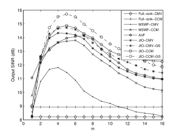
Fig. 2: Output SINR versus the number of snapshots with $\mu_{T_{r}}=0.002$, $\mu_{\bar{w}}=0.001$, $\mu_{T_{r},\textrm{gs}}=0.003$, $\mu_{\bar{w},\textrm{gs}}=0.0007$.

In Fig. 3, we keep the same scenario as that in Fig. 2 and check the rank selection for the existing and proposed algorithms. The number of snapshots is fixed to $N=500$. The most adequate rank values for the proposed algorithms are $r=r_{\textrm{gs}}=5$, which are comparatively lower than most existing algorithms, but reach the preferable performance. We also checked that these values are rather insensitive to the number of users in the system, to the number of sensor elements, and work efficiently for the studied scenarios.

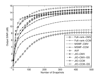
Fig. 3: Output SINR versus dimension ($m$) with $\mu_{T_{r}}=0.002$, $\mu_{\bar{w}}=0.001$, $\mu_{T_{r},\textrm{gs}}=0.003$, $\mu_{\bar{w},\textrm{gs}}=0.0007$.

Finally, the mismatch (steering vector error) condition is analyzed in Fig. 4. The number of users is $q=10$, including one desired user. In Fig. 4(a), the exact DOA of the SOI is known at the receiver. The output performance of the proposed algorithms is better than those of the existing methods, and the convergence is a little slower than that of the AVF algorithm, but faster than the others. In Fig. 4(b), we set the DOA of the SOI estimated by the receiver to be $2^{\textit{o}}$ away from the actual direction. It indicates that the mismatch problem induces performance degradation to all the analyzed algorithms. The CCM-based methods are more robust to this scenario than the CMV-based ones. The proposed algorithms still retain outstanding performance compared with other techniques.

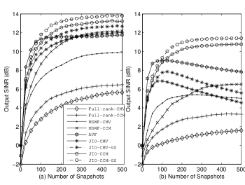
Fig. 4: Output SINR versus the number of snapshots with $\mu_{T_{r}}=0.002$, $\mu_{\bar{w}}=0.001$, $\mu_{T_{r},\textrm{gs}}=0.003$, $\mu_{\bar{w},\textrm{gs}}=0.0007$ for (a) ideal steering vector condition; (b) steering vector mismatch $2^{o}$.

6 Concluding Remarks

We proposed a CCM reduced-rank scheme based on the joint iterative optimization of adaptive filters for beamforming and devised two efficient algorithms, namely, JIO-CCM and JIO-CCM-GS, for implementation. The transformation matrix and reduced-rank weight vector are jointly estimated to get the filter output. By using the GS technique to reformulate the transformation matrix, the JIO-CCM-GS algorithm achieves faster convergence and better performance than the JIO-CCM. The devised algorithms, compared with the existing methods, show preferable performance in the studied scenarios.

References

- [1]
- [2] J. Litva and T. K. Lo, Digital Beamforming in Wireless Communications, Artech House, 1996.
- [3] H. L. Van Trees, Detection, Estimation, and Modulation, Part IV, Optimum Array Processing,” John Wiley & Sons, 2002.
- [4] J. Li and P. Stoica, Robust Adaptive Beamforming, Hoboken, NJ: Wiley, 2006.
- [5] O. L. Frost, “An algortihm for linearly constrained adaptive array processing,” IEEE Proc., AP-30, pp. 27-34, 1972.
- [6] R. C. de Lamare and R. Sampaio-Neto, “Low-complexity variable step-size mechanisms for stochastic gradient algorithms in minimum variance CDMA receivers,” IEEE Trans. Signal Processing, vol. 54, pp. 2302-2317, June 2006.
- [7] L. Wang and R. C. de Lamare, “Constrained adaptive filtering algorithms based on conjugate gradient techniques for beamforming,” IET Signal Processing , vol.4, no.6, pp.686-697, Dec. 2010.
- [8] S. Haykin, Adaptive Filter Theory, 4rd ed., Englewood Cliffs, NJ: Prentice-Hall, 1996.
- [9] J. R. Guerci, J. S. Goldstein, and I. S. Reed, “Optimal and adaptive reduced-rank STAP,” IEEE Trans. Aerospace and Electronic Systems, vol. 36, pp. 647-663, Apr. 2000.
- [10] M. L. Honig and W. Xiao, “Performance of reduced-rank linear interference suppression,” IEEE Trans. Information Theory, vol. 47, pp. 1928-1946, July 2001.
- [11] J. S. Goldstein, I. S. Reed, and L. L. Scharf, “A multistage representation of the wiener filter based on orthogonal projections,” IEEE Trans. Information Theory, vol. 44, pp. 2943-2959, Nov. 1998.
- [12] M. L. Honig and J. S. Goldstein, “Adaptive reduced-rank interference suppression based on the multistage wiener filter,” IEEE Trans. Communications, vol. 50, pp. 986-994, June 2002.
- [13] R. C. de Lamare, M. Haardt, and R. Sampaio-Neto, “Blind adaptive constrained reduced-rank parameter estimation based on constant modulus design for CDMA interference suppression,” IEEE Trans. Signal Proc., vol. 56, pp. 2470-2482, Jun. 2008.
- [14] D. A. Pados and S. N. Batalama, “Joint space-time auxiliary-vector filtering for DS/CDMA systems with antenna arrays,” IEEE Trans. Commun., vol. 47, pp. 1406-1415, Sep. 1999.
- [15] D. A. Pados and G. N. Karystinos, “An iterative algorithm for the computation of the MVDR filter,” IEEE Trans. Signal Processing, vol. 49, pp. 290-300, Feb. 2001.
- [16] R. C. de Lamare and R. Sampaio-Neto, “Adaptive Reduced-Rank MMSE Filtering with Interpolated FIR Filters and Adaptive Interpolators”, IEEE Sig. Proc. Letters, vol. 12, no. 3, March, 2005.
- [17] R. C. de Lamare and Raimundo Sampaio-Neto, “Reduced-rank Interference Suppression for DS-CDMA based on Interpolated FIR Filters”, IEEE Communications Letters, vol. 9, no. 3, March 2005.
- [18] R. C. de Lamare and R. Sampaio-Neto, “Adaptive Interference Suppression for DS-CDMA Systems based on Interpolated FIR Filters with Adaptive Interpolators in Multipath Channels”, IEEE Transactions on Vehicular Technology, Vol. 56, no. 6, September 2007.
- [19] R. C. de Lamare and R. Sampaio-Neto, “Reduced-Rank Adaptive Filtering Based on Joint Iterative Optimization of Adaptive Filters, ” IEEE Signal Processing Letters, Vol. 14 No. 12, December 2007, pp. 980 - 983.
- [20] R. C. de Lamare, “Adaptive reduced-rank LCMV beamforming algorithms based on joint iterative optimization of filters,” Electronics Letters, vol. 44, no. 9, Apr. 2008.
- [21] R. C. de Lamare and R. Sampaio-Neto, “Adaptive Reduced-Rank Processing Based on Joint and Iterative Interpolation, Decimation and Filtering”, IEEE Transactions on Signal Processing, vol. 57, no. 7, July 2009, pp. 2503 - 2514.
- [22] G. H. Golub and C. F. Van Loan, Matrix Comuputations, 3rd ed. Baltimore, MD: Johns Hopkins Univ. Press, 1996.
- [23]