Two defect lines separated by a distance $\delta$ look from much larger distances like a single defect. In the critical theory, when all scales are large compared to the cutoff scale, this fusion of defect lines is universal. We calculate the universal fusion rule in the critical 2D Ising model and show that it is given by the Verlinde algebra of primary fields, combined with group multiplication in $O(1,1)/Z_{2}$. Fusion is in general singular and requires the subtraction of a divergent Casimir energy.

1 Introduction and Summary

Ever since Onsager’s celebrated solution [1], the two-dimensional Ising model has been the prototype for the study of second-order phase transitions. The model also exhibits critical behavior on boundaries [2], and on defect lines. The latter have been analyzed using both integrability ([3, 4] and references therein) and conformal field theory [5, 6] techniques. It has been found, in particular, that the critical behavior of defect lines is captured by the three continuous families given in table 1.

The purpose of the present note is to compute the fusion algebra [7] of these conformal defects: when two of them are placed parallel to each other, they fuse to another such defect line in the limit of zero separation. The process is in general singular, and requires the subtraction of a divergent self-energy.

It turns out that the resulting fusion algebra takes a simple form in the fermionic representation of the Ising model. There, defect lines are parametrized by a gluing matrix $\Lambda\equiv-\Lambda\in O(1,1)/\mathbb{Z}_{2}$ of the fermions, which has to be an element of the Lorentz group in 1+1 dimensions (modulo its center), and by an Ising primary $a\in\{\boldsymbol{1}$, $\boldsymbol{\epsilon},\boldsymbol{\sigma}\}$. Defect fusion then reduces to a combination of multiplication in the Lorentz group, and multiplication in the Verlinde algebra of the Ising model ($\boldsymbol{1}\times a=a$, $\boldsymbol{\epsilon}\times\boldsymbol{\epsilon}=\boldsymbol{1}$, $\boldsymbol{\epsilon}\times\boldsymbol{\sigma}=\boldsymbol{\sigma}$ and $\boldsymbol{\sigma}\times\boldsymbol{\sigma}=\boldsymbol{1}+\boldsymbol{\epsilon}$, see e.g. [8]). Explicitly, defects associated to $(a,\Lambda)$ and $(a^{\prime},\Lambda^{\prime})$ fuse according to

$$(a,\Lambda)\star(a^{\prime},\Lambda^{\prime})=(a\times a^{\prime},\Lambda\Lambda^{\prime})\,.$$ (1)

For the special subclass of defects with diagonal gluing matrix $\Lambda$ fusion was previously obtained in [9]. These are topological defects and their fusion is non-singular. Here, using the results of [10], we will derive fusion of general conformal defect lines in the Ising model, i.e. of all defects obtained by marginal deformations of the topological defect lines.

Spin-chain defect	$\mathbb{Z}_{2}$-orbifold boundary	Fermionic
ferromagnetic, $b\in(0,\infty)$	Dirichlet, $\phi_{0}\in(0,\pi/2)$	$\mathbf{1}$, ${\rm det}\Lambda=1$
anti-ferromagnetic, $b\in(-\infty,0)$	Dirichlet, $\phi_{0}\in(\pi/2,\pi)$	$\boldsymbol{\epsilon}$, ${\rm det}\Lambda=1$
order-disorder, $\tilde{b}\in(0,\infty)$	Neumann, $\tilde{\phi}_{0}\in(0,\pi/2)$	$\boldsymbol{\sigma}$, ${\rm det}\Lambda=-1$

Table 1: Universality classes of defect lines in the Ising model. The left column gives the natural parametrization in terms of Ising spins. The central one the corresponding boundary states in the $c=1$ CFT. Finally the right column gives the parametrization in terms of gluing matrices for the fermion fields and Ising primaries.

The Ising model on a square lattice with an integrable, ferromagnetic or anti-ferromagnetic defect line has the energy-to-temperature ratio

$${{\cal E}\over T}=-\sum_{i,j}(K_{1}\sigma_{i,j}\sigma_{i+1,j}+K_{2}\sigma_{i,j}\sigma_{i,j+1})+(1-b)K_{1}\sum_{j}\sigma_{0,j}\sigma_{1,j}$$ (2)

where $\sigma_{i,j}=\pm 1$ are the spin variables, and ${\rm sinh}(2K_{1})\,{\rm sinh}(2K_{2})=1$ in order for the bulk theory to be critical. Couplings along the (vertical) defect line are rescaled by a factor $b$, which parametrizes marginal deformations of the defect. These defects correspond to conformal defect lines specified by Ising primaries $a\in\{\boldsymbol{1},\boldsymbol{\epsilon}\}$ and fermion-gluing matrices

$$\Lambda=\left(\begin{array}[]{cc}{\rm cosh}\gamma&{\rm sinh}\gamma\\ {\rm sinh}\gamma&{\rm cosh}\gamma\end{array}\right)\$$ (3)

of determinant 1, c.f. table 1. As we will see, the relation between the defect strength $b$ and the hyperbolic angle $\gamma$ of the gluing matrix is given by

$$\gamma={\rm log}\Bigl{|}{{\rm tanh}(bK_{1})\over{\rm tanh}(K_{1})}\Bigr{|}\ .$$ (4)

Since the Lorentz matrices (3) multiply by adding the hyperbolic angles $\gamma$, the fusion of two defects with couplings $b$ and $b^{\prime}$ results in a defect with coupling $b^{\prime\prime}$, where

$${\rm tanh}(b^{\prime\prime}K_{1})\,{\rm tanh}(K_{1})={\rm tanh}(bK_{1})\,{\rm tanh}(b^{\prime}K_{1})\ .$$ (5)

Notice that we wrote the fusion rule without the absolute values coming from (4). Indeed, the signs of the defect strengths combine multiplicatively, in accordance with the $Z_{2}$ algebra of the Ising primaries $\boldsymbol{1}$ and $\boldsymbol{\epsilon}$.

The Ising model also features order-disorder defects which are obtained by performing a duality transformation on one side of the (anti-)ferromagnetic defect lines. As detailed in table 1, these correspond to the conformal defects with $a=\boldsymbol{\sigma}$ and fermion gluing matrix

$$\tilde{\Lambda}=\left(\begin{array}[]{cc}{\rm cosh}\tilde{\gamma}&-{\rm sinh}\tilde{\gamma}\\ {\rm sinh}\tilde{\gamma}&-{\rm cosh}\tilde{\gamma}\end{array}\right)\$$ (6)

of determinant $-1$. The microscopic realization of these defect lines is most simple in the strongly-anisotropic limit of the critical Ising model, $K_{1}\to 0$ (which implies $K_{2}\to\infty$). In this limit one has

$$e^{\gamma}=|b|\qquad{\rm and}\qquad e^{\tilde{\gamma}}=\tilde{b}\ ,$$ (7)

where $\tilde{b}$ is the coupling strength of the order-disorder defect.

The fusion of two order-disorder defects turns out to produce the sum of a ferromagnetic and an anti-ferromagnetic defect of the same absolute strength $|b^{\prime\prime}|$. Since the Lorentz matrices (6) multiply by subtracting the hyperbolic angles, one finds

$$|b^{\prime\prime}|=\tilde{b}/\tilde{b}^{\prime}\ .$$ (8)

Notice that two order-disorder defects only commute if they are identical. Likewise the fusion of an (anti-)ferromagnetic with an order-disorder defect line produces an order-disorder defect line with coupling

$$\tilde{b}^{\prime\prime}=|b|\,\tilde{b}^{\prime}\qquad{\rm or}\qquad\tilde{b}^{\prime\prime}=\tilde{b}/|b^{\prime}|\ ,$$ (9)

depending on whether the (anti-)ferromagnetic defect is fused from the left or the right. Defect fusion is non-commutative.

The above rules for fusion of defect lines are the main results of this letter. They are summarized by the master formula (1). We should stress that although the fusion algebra is universal, the parametrization of the critical lines of defects is not. In particular, relation (4) depends on the non-universal constant $K_{1}$. Note also that the stability of the order-disorder defects is ensured by a $\mathbb{Z}_{2}\times\mathbb{Z}_{2}$ symmetry, which reflects separately the spins on the two sides of the defect line, whereas the more stable (anti-)ferromagnetic defects only preserve the diagonal $\mathbb{Z}_{2}$ [6].

2 Fusion of Conformal Defects

Figure 1 illustrates the physical meaning of fusion of conformal defects: we consider two defect lines ${\cal D}$ and ${\cal D}^{\prime}$ separated by a distance $\delta$, and let $x$ be the typical (horizontal) scale at which the system is probed. For $x\gg\delta$ the system flows to an effective defect line ${\cal D}_{\rm eff}$, but in general this ${\cal D}_{\rm eff}$ will depend on $\delta$ and on the precise microscopic realization of the defects ${\cal D}$ and ${\cal D}^{\prime}$. Put differently, the composition of two defects for finite $\delta$ is not universal. If, however, $\delta$ is also large compared to the lattice spacing $\Delta$, then one expects the fusion to only depend on the universality classes of ${\cal D}$ and ${\cal D}^{\prime}$. This universal composition rule can be calculated in conformal theory.

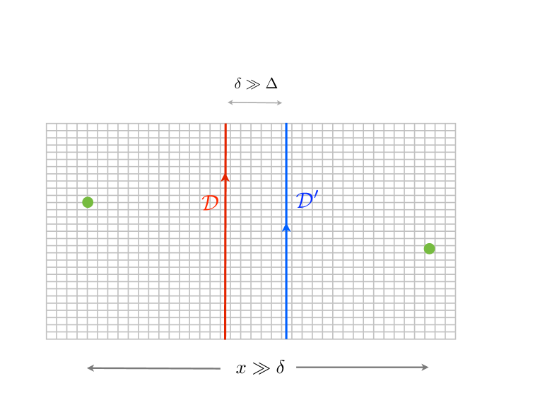
Figure 1: The two-defect system discussed in the text. The green dots are arguments of a typical two-point function at a horizontal scale $x\gg\delta$. The fusion product ${\cal D}\star{\cal D}^{\prime}$ gives an effective description of this system in the limit where $\delta$ is very large compared to the lattice spacing $\Delta$. Only in this limit is fusion universal.

To perform the calculation, one may quantize the CFT by compactifying the defect line on a circle and treating the normal direction as time. The defect is then described by a formal operator which acts on the space of states of the CFT on the circle. This generalizes the technical device of boundary state [11] to defect lines. The action of two coincident defects is given by the product of the corresponding operators, but this is in general singular and requires regularization and renormalization.

A simple example, that of $U(1)^{2}$ invariant defects in the $c=1$ CFT [12], has been worked out in detail in reference [7]. In this case a single subtraction of a divergent Casimir energy is sufficient to render the result finite, so one defines

$${\cal D}\star{\cal D}^{\prime}={\rm lim}_{\delta\to 0}\ [e^{-C/\delta}\,{\cal D}\,e^{-\delta\,{\cal H}}\,{\cal D}^{\prime}]\ ,$$ (10)

where ${\cal H}$ is the CFT Hamiltonian, and $C/\delta$ is the Casimir energy. Here we use the same symbol for a defect line and for the corresponding operator. Note that the divergent (or vanishing) factor $e^{-C/\delta}$ is an overall normalization that drops out of the calculation of correlation functions.

The analysis of [7] was recently extended to many free bosons and fermions in reference [10]. Since the $c=1/2$ CFT is the theory of a free fermion, all we have to do is to translate the relevant calculations of the latter reference to the language of the Ising model.

3 Conformal defects of the Ising model

The critical defect lines of the Ising model can be mapped, using the folding trick, to boundary conditions in the $c=1$ orbifold theory [5, 6]. The idea is illustrated in figure 2: the $\mathbb{Z}_{2}$ orbifold of a free boson on a circle describes the critical line of the Ashkin-Teller model. It reduces to two decoupled Ising models when the radius of the circle is $r=1$ [15]. Unfolding converts any boundary condition of the $r=1$ orbifold to a defect line of the Ising model, and vice versa, whence the equivalence.

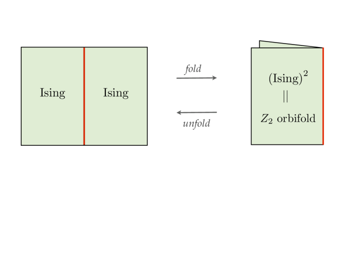
Figure 2: Folding transforms defect lines (in red) of the critical Ising model to boundary conditions of the $c=1$ $\mathbb{Z}_{2}$-orbifold theory.

As explained in [5, 6], see also [16], the conformal boundary conditions of the orbifold theory come in two continuous families:

• the Dirichlet condition $|D,\phi_{0}\,\rangle\hskip-1.5649pt\rangle$ with $\phi_{0}\in[0,\pi]$, and

• the Neumann condition $|N,\tilde{\phi}_{0}\,\rangle\hskip-1.5649pt\rangle$ with $\tilde{\phi}_{0}\in[0,\pi/2]$.

In the language of string theory, $\phi_{0}$ is the position of a D0-brane on the circle, modulo the $\mathbb{Z}_{2}$ identification, whereas $\tilde{\phi}_{0}$ is the Wilson line on a D1-brane, or equivalently the position of the dual D0-brane on the dual circle (of radius $\tilde{r}=1/2$). Here we have specified the boundary conditions by means of the corresponding boundary states $|{\cal B}\,\rangle\hskip-1.5649pt\rangle$. Unfolding converts the boundary states of (Ising)² to defect operators of the Ising model.

The relation between $\phi_{0}$ and the parameter $b$ of the “defective” model (2) has been obtained in [5, 6] by comparing the CFT spectrum with the exact diagonalization of the transfer matrix [4, 17]:

$${\rm tan}(\phi_{0}-{\pi\over 4})={{\rm sinh}(K_{1}(1-b))\over{\rm sinh}(K_{1}(1+b))}\ \Longleftrightarrow\ {\rm cot}\phi_{0}=\,{{\rm tanh}(bK_{1})\over{\rm tanh}(K_{1})}\ .$$ (11)

Note that $\phi_{0}=\pi/4$ corresponds to $b=1$, i.e. to no defect. The corresponding operator is the identity operator. Another special value is $\phi_{0}=3\pi/4$, which corresponds to $b=-1$. This defect line can be removed by flipping the signs of all spins on one side of the defect.

Three other special values are $\phi_{0}=0,\pi/2$ and $\pi$, corresponding to $b=\infty,0$ and $-\infty$ respectively. At these special values the defect line reduces to separate boundary conditions for the two Ising models, namely

$$(++)\oplus(--)\ ,\ \ (ff)\ \ {\rm and}\ \ (+-)\oplus(-+)\ ,$$ (12)

where $(+),(-),(f)$ denote the three conformal boundary conditions of the Ising model: spin-up, spin-down and free [18].

In the infinitely anisotropic limit, $K_{1}\to 0$ and ${\rm sinh}(2K_{2})\simeq 1/2K_{1}\to\infty$, the critical Ising model with a defect line of Dirichlet type can be described equivalently by the quantum-spin chain with Hamiltonian [3]

$$H_{D}=-\sum_{n}\,h^{*}\sigma_{n}^{x}-\sum_{n\not=0}\sigma_{n}^{z}\sigma_{n+1}^{z}-b\,\sigma_{0}^{z}\sigma_{1}^{z}\ ,$$ (13)

where $h^{*}=1$ is the critical value of the transverse magnetic field. The defect sits on the link $\langle 01\rangle$ of the spin chain, and this Hamiltonian describes the evolution in the direction parallel (not transverse) to the defect line. The coupling at the defective link is $b={\rm cot}\phi_{0}$.

In the quantum spin-chain language one can also describe the Neumann family of conformal defects whose Hamiltonian is [6]

$$H_{N}=-\sum_{n}\,h^{*}\sigma_{n}^{x}-\sum_{n\not=0}\sigma_{n}^{z}\sigma_{n+1}^{z}-\tilde{b}\,\sigma_{0}^{z}\sigma_{1}^{x}\ .$$ (14)

Here again $\tilde{b}={\rm cot}\tilde{\phi}_{0}$, but one may now restrict $\tilde{b}\geq 0$, so that $\tilde{\phi}_{0}$ only takes values in the interval $[0,\pi/2]$. This follows from the automorphism of the Pauli matrices $(\sigma^{x},\sigma^{y},\sigma^{z})\to(\sigma^{x},-\sigma^{y},-\sigma^{z})$ which flips the sign of $\tilde{b}$ while leaving the bulk Hamiltonian unchanged.

The nature of the Neumann defects is made transparent by a Kramers-Wannier duality of the half-chain $n>0$. This maps $\sigma_{1}^{x}$ to $\mu_{1}^{z}$, where $\vec{\mu}_{n}$ are the disorder operators, and the Neumann defect to an order-disorder coupling of the two half-chains [6]. When $\tilde{\phi}_{0}=\pi/4$ we have $\tilde{b}=1$, and the Neumann defect is topological; it implements the order-disorder duality in the $c=1/2$ conformal field theory [21]. At the endpoints $\tilde{\phi}_{0}=0,\pi/2$ on the other hand the defect reduces to the separate boundary conditions

$$(+f)\oplus(-f)\ \ \ {\rm and}\ \ (f+)\oplus(f-)\ .$$ (15)

Two interesting quantities that characterize all conformal defects are the ground-state degeneracy $g$ [22] and the reflection coefficient ${\cal R}$, given by the 2-point function of the energy momentum tensor [16]

$${\cal R}:={\langle T_{1}\bar{T}_{1}+T_{2}\bar{T}_{2}\rangle\over\langle(T_{1}+\bar{T}_{2})(\bar{T}_{1}+T_{2})\rangle}\ .$$ (16)

Here, $T_{1},\bar{T}_{1}$ are the components of the energy-momentum tensor at any point $z$, while $T_{2},\bar{T}_{2}$ are evaluated at the point obtained by reflection with respect to the defect line. For the defects of interest here one finds:

$$\underline{\rm Dirichlet}:\ \ g=1\ ,\ \ {\cal R}={\rm cos}^{2}(2\phi_{0})$$

$$\underline{\rm Neumann}:\ \ g=\sqrt{2}\ ,\ \ {\cal R}={\rm cos}^{2}(2\tilde{\phi}_{0})\ .$$ (17)

Note that at $\phi_{0}=n\pi/2$, where the Dirichlet defect reduces to totally-reflecting boundary conditions, the reflection coefficient is ${\cal R}=1$. Conversely, at $\phi_{0}=\pi/4$ or $3\pi/4$ the defect is topological and there is no reflection, ${\cal R}=0$. Similar statements hold for the Neumann defects.

4 Folding-unfolding dictionary

In order to calculate the fusion product defined in (10) we need to unfold the boundary states of the orbifold theory to defect operators acting on the space of states of the Ising model. The critical Ising model is described by a free massless fermion field with components

$$(\psi,\bar{\psi})=\sum_{r}\ (\psi_{r}e^{-r(\tau+i\sigma)}\ ,\ \bar{\psi}_{r}e^{-r(\tau-i\sigma)})\ .$$ (18)

Here, $z=\tau+i\sigma$ parametrizes the cylinder $\mathbb{R}\times[0,2\pi]$, and the Fourier modes satisfy the canonical anticommutation relations $\{\psi_{r},\psi_{s}\}=\{\bar{\psi}_{r},\bar{\psi}_{s}\}=\delta_{r+s,0}\ .$ The left and right components of the energy-momentum tensor are given by

$$T=-{1\over 2}:\hskip-1.99168pt\psi\,\partial\psi\hskip-1.42262pt:\ \ \ {\rm and}\ \ \ \bar{T}=-{1\over 2}:\hskip-1.99168pt\bar{\psi}\,\bar{\partial}\bar{\psi}\hskip-1.42262pt:\ ,$$ (19)

where $\partial\equiv\partial/\partial z$, $\bar{\partial}\equiv\partial/\partial\bar{z}$, and the double dots stand for normal ordering.

The fermion can be antiperiodic (Neveu-Schwarz) or periodic (Ramond), and we denote the corresponding ground states by $|0\rangle_{\rm NS}$ and $|0,{\scriptstyle{A}}\rangle_{\rm R}$, ${\scriptstyle{A}}=\pm$. The two Ramond ground states represent the Dirac algebra of the zero modes $\psi_{0}$ and $\bar{\psi}_{0}$. The Ising CFT can be obtained from the free fermonic theory by a projection onto even fermion parity which acts as a chiral projection on the Ramond ground states. This in particular lifts the ground state degeneracy in the Ramond sector. The three primary fields of the Ising model $\boldsymbol{1},\boldsymbol{\epsilon}$ and $\boldsymbol{\sigma}$, are mapped by the operator-state correspondence to the states $|0\rangle_{\rm NS}$, $\psi_{-1/2}\bar{\psi}_{-1/2}|0\rangle_{\rm NS}$ and $|0,+\rangle_{\rm R}$, respectively.

Consider now a defect placed on the circle $\tau=0$ around the cylinder. Conformal invariance is tantamount to continuity of $T-\bar{T}$. Equivalently, the Fourier modes

$$\int_{0}^{2\pi}{d\sigma\over 2\pi}\,e^{iN\sigma}\ (T-\bar{T})\,=\,{1\over 2}\sum_{r}({r}+{N\over 2})(:\hskip-1.99168pt\psi_{-r}\psi_{N+r}\hskip-1.42262pt:+:\hskip-1.99168pt\bar{\psi}_{r}\bar{\psi}_{-N-r}\hskip-1.42262pt:)\$$ (20)

on both sides of the defect line have to agree. This is obviously guaranteed by the gluing conditions 

$$\left(\begin{array}[]{c}\psi_{-r}\\ \\ -i\,\bar{\psi}_{r}\end{array}\right)\,{\cal D}\,=\,{\cal D}\,\Lambda\left(\begin{array}[]{c}\psi_{-r}\\ \\ -i\,\bar{\psi}_{r}\end{array}\right)\ ,$$ (21)

provided $\Lambda$ is an element of $O(1,1)$, the group of Lorentz transformations in 1+1 dimensions, i.e. $\Lambda^{t}\eta\Lambda=\eta$ for $\eta={\rm diag}(1,-1)$. In the above equation ${\cal D}$ is the defect operator, and the mode operators acting on the left and right of it come from fields on the left ($\tau<0$) and right ($\tau>0$) of the defect line respectively.

To relate (21) to the boundary states of the previous section we must fold the half-cylinder $\tau>0$, so that we now have two fermions at $\tau<0$. Time reflection exchanges left- and right-movers,

$$\left(\begin{array}[]{c}\psi_{r}\\ \bar{\psi}_{r}\end{array}\right)\to\left(\begin{array}[]{c}-i\bar{\psi}_{-r}\\ i\psi_{-r}\end{array}\right)\ ,$$ (22)

and a little algebra allows us to convert (21) into a boundary condition for the two-fermion theory [10]

$$\left[\left(\begin{array}[]{c}\psi^{1}_{r}\\ \psi^{2}_{r}\end{array}\right)+i\mathcal{O}\left(\begin{array}[]{c}\bar{\psi}^{1}_{-r}\\ \bar{\psi}^{2}_{-r}\end{array}\right)\right]|{\cal B}\,\rangle\hskip-1.42262pt\rangle\,=\,0\,,$$ (23)

where $\mathcal{O}$ is the 2$\times$2 rotation matrix

$$\mathcal{O}(\Lambda)=\left(\begin{array}[]{cc}\Lambda_{12}\Lambda_{22}^{-1}&\Lambda_{11}-\Lambda_{12}\Lambda_{22}^{-1}\Lambda_{21}\\ \Lambda_{22}^{-1}&-\Lambda_{22}^{-1}\Lambda_{21}\end{array}\right)\,.$$ (24)

Equation (24) maps the Lorentzian group $O(d,d)$ to the rotation group $O(2d)$ for any $d$, but we will only need it for $d=1$ here.

The group $O(1,1)$ has four connected components containing the four elements $\Lambda={\rm diag}(\pm 1,\pm 1)$ respectively. Due to the projection onto even fermion parity, $\Lambda$ and $-\Lambda$ describe equivalent gluings so that there are only two continuous families of gluing conditions. The ones with ${\rm det}\Lambda=+1$ correspond to the Dirichlet boundary conditions in the orbifold theory, i.e. to the (anti-)ferromagnetic defect lines, whereas the ones with ${\rm det}\Lambda=-1$ correspond to the Neumann boundary conditions, i.e. to the order-disorder defect lines.

To establish the exact dictionary, we first use (24) to relate the gluing matrix $\Lambda$ (for ${\rm det}\Lambda=+1$) to the following rotation matrix:

$$\Lambda=\left(\begin{array}[]{cc}{\rm cosh}\gamma&{\rm sinh}\gamma\\ {\rm sinh}\gamma&{\rm cosh}\gamma\end{array}\right)\ \leftrightarrow\ \mathcal{O}=\left(\begin{array}[]{cc}{\rm cos}(2\phi_{0})&{\rm sin}(2\phi_{0})\\ {\rm sin}(2\phi_{0})&-{\rm cos}(2\phi_{0})\end{array}\right)\ ,$$ (29)

where

$${\rm cos}(2\phi_{0})={\rm tanh}\gamma\ \ \Longleftrightarrow\ \ e^{\gamma}={\rm cot}\phi_{0}\ .$$ (30)

The bosonization formulae $\psi^{1}+i\psi^{2}={\rm exp}(2\int\partial\phi)$ and $\bar{\psi}^{2}+i\bar{\psi}^{1}={\rm exp}(2\int\bar{\partial}\phi)$, and the boundary condition (23) allow us to identify the angle $\phi_{0}$ with the D0-brane position on the orbifold space. As $\gamma$ ranges from $\infty$ to $-\infty$, $\phi_{0}$ takes values in $[0,\pi/2]$. However, gluing in the Ramond sector involves the spinor representation $S(\mathcal{O})$ of the orthogonal group $O(2)$. This effectively doubles the range of $\phi_{0}$, in agreement with the discussion of section 3: the defects with $\phi_{0}\in[0,\pi/2]$ correspond to defects with $a=\boldsymbol{1}$, whereas the ones with $\phi_{0}\in[\pi/2,\pi]$ correspond to defects with $a=\boldsymbol{\epsilon}$.

Combining equations (30) and (11) yields relation (4) between the Ising model parameter $b$ and the hyperbolic angle $\gamma$ quoted in the introduction.

The gluing conditions (21) with ${\rm det}\Lambda=-1$ fold to boundary gluings (23), with the following O(2) matrix:

$$\Lambda=\left(\begin{array}[]{cc}{\rm cosh}\tilde{\gamma}&-{\rm sinh}\tilde{\gamma}\\ {\rm sinh}\tilde{\gamma}&-{\rm cosh}\tilde{\gamma}\end{array}\right)\ \ \leftrightarrow\ \mathcal{O}=\left(\begin{array}[]{cc}{\rm cos}(2\tilde{\phi}_{0})&{\rm sin}(2\tilde{\phi}_{0})\\ -{\rm sin}(2\tilde{\phi}_{0})&{\rm cos}(2\tilde{\phi}_{0})\end{array}\right)\ ,$$ (35)

where $\tilde{\gamma}$ is related to $\tilde{\phi}_{0}$ as in (30). Since transformations with ${\rm det}\Lambda=-1$ flip the chirality of $O(1,1)$ spinors, such defect operators cannot act consistently in the Ramond sector [10]. As a result, one may restrict $\tilde{\phi}_{0}\in[0,\pi/2]$.

The boundary states obeying conditions (23) were constructed explicitly and unfolded into defect operators in reference [10]. In a somewhat elliptical notation they read:

$${\cal D}^{\pm}\ =\ {\cal T}(\prod_{r>0}e^{-i\sum_{j,k}\mathcal{O}_{jk}\psi^{j}_{-r}\bar{\psi}^{k}_{-r}}){1\over 2}\Bigl{[}\mathbb{I}_{0}^{\rm NS}\,\pm\,{1\over\sqrt{{\rm cosh}\gamma}}\,\mathbb{I}_{0}^{\rm R}\,S(\Lambda)\Bigr{]}\ +\ (\Lambda\mapsto-\Lambda)\$$

$${\rm and}\ \ \ \ \ \tilde{\cal D}=\,\ {\cal T}(\prod_{r>0}e^{-i\sum_{j,k}\mathcal{O}_{jk}\psi^{j}_{-r}\bar{\psi}^{k}_{-r}}){1\over\sqrt{2}}\,\mathbb{I}_{0}^{\rm NS}\ +\ (\Lambda\mapsto-\Lambda)\ ,$$

where

$$\mathbb{I}_{0}^{\rm NS}=|0\rangle_{\rm NS}\ {}_{\rm NS}\langle 0|\qquad{\rm and}\qquad\mathbb{I}_{0}^{\rm R}=\sum_{\scriptstyle{A}}|0,{\scriptstyle{A}}\rangle_{\rm R}\ {}_{\rm R}\langle 0,{\scriptstyle{A}}|$$ (36)

are the identity operators in the ground-state sectors. ${\mathcal{D}}^{\pm}$ are the defect operators for ${\rm det}\Lambda=+1$ and $\tilde{\mathcal{D}}$ the ones for ${\rm det}\Lambda=-1$. Furthermore $\mathcal{O}$ is the orthogonal matrix given in (24), and the oscillator frequencies $r$ run over the positive integers or half-integers in the periodic, respectively antiperiodic sectors. Finally ${\cal T}$ is the time-reversal operation (22) which acts only on the $j=2$ fermions, i.e. on the copy of the Ising CFT that is being unfolded.

The meaning of the above formulae is as follows: expand the exponentials, apply the operation ${\cal T}$, and act by the fermion modes with index $j=1$ on the left and those with index $j=2$ on the right of the ground-state isomorphisms $\mathbb{I}_{0}^{\rm NS}$ or $\mathbb{I}_{0}^{\rm R}$.

In the notation of the introduction we have the following correspondence between defect lines and operators:

$$(\boldsymbol{1},\Lambda)\mapsto{\cal D}^{+}(\Lambda)\ ,\;(\boldsymbol{\epsilon},\Lambda)\mapsto{\cal D}^{-}(\Lambda)\qquad {\rm for} \qquad{\rm det}\Lambda=1$$

$${\rm and}\qquad(\boldsymbol{\sigma},\Lambda)\mapsto\tilde{\cal D}(\Lambda)\qquad {\rm for} \qquad{\rm det}\Lambda=-1\ .$$ (37)

The translation in the language of the Ising model was given in table 1.

The order-disorder defect $\tilde{\cal D}$ has no Ramond component. Since the spin operator is in the Ramond sector, we conclude that there is no correlation between spin operators on either side of such defect lines.

5 Computing the fusion

Having constructed the defect operators, we can now compute the fusion of defects as defined in (10). This was done (for any number of fermion fields) in [10]. We will recall the main steps of this calculation here.

Note first that all defect operators are (sums of) products of the form

$${\cal D}=\,{\cal D}_{0}\,\prod_{r>0}{\cal D}_{r}\ ,$$ (38)

where ${\cal D}_{r}$ only involves the fermion modes $\psi_{\pm r}^{j}$ and $\bar{\psi}_{\pm r}^{j}$, while ${\cal D}_{0}$ gives the action of the defect operator on the ground states. The operators ${\cal D}_{r}$ for different $r$ commute, so their order is irrelevant. Hence, in evaluating the product in (10), we may consider each term ${\cal D}_{r}e^{-\delta{\cal H}}{\cal D}^{\prime}_{r}$ separately.

We use the label $j=1,2,3$ to denote the fermion field in the region on the left of both defects, in the region between the two defects, and finally the region on the right (see figure 2). Thus, the operator ${\cal D}$ involves the fermions $j=1,2$ and ${\cal D}^{\prime}$ the fermions $j=2,3$. Now the idea is to anticommute the common fermions, $j=2$, so as to bring all positive-frequency (annihilation) operators to the right of all negative-frequency (creation) operators. The result can then be easily evaluated, since it is sandwitched between ground states of theory 2. One ends up with an expression that only involves the fermions $j=1,3$, which are spectators in this rearrangement.

To perform this calculation we use the following identities:

$$e^{\chi\psi_{r}}\,f(\psi_{-r})\,=\,f(\psi_{-r}+\chi)\,e^{\chi\psi_{r}}\ ,$$ (39)

valid for any function $f$ and any operator $\chi$ that anticommutes with the $\psi_{\pm r}$, and

$$\langle 0|\ e^{u\,\psi_{r}\bar{\psi}_{r}}\,e^{u^{\prime}\psi_{-r}\bar{\psi}_{-r}}=(1-u\,u^{\prime})\,\langle 0|\,{\rm exp}\left({u\over 1-u\,u^{\prime}}\,\psi_{r}\bar{\psi}_{r}\right)\ ,$$ (40)

where $u,u^{\prime}$ are c-numbers. Consider two defects with gluing matrices $\Lambda$ and $\Lambda^{\prime}$ and corresponding orthogonal matrices $\mathcal{O}$ and $\mathcal{O}^{\prime}$. Using the above identities leads after some tedious algebra to [10]

$${\cal D}_{r}e^{-\delta{\cal H}}{\cal D}^{\prime}_{r}\ =\ (1-e^{-2\delta r}\mathcal{O}_{11}^{\prime}\mathcal{O}_{22})\,{\cal T}(e^{-i\sum_{j,k}\mathcal{O}_{jk}^{\prime\prime}(e^{-2\delta r})\psi^{j}_{-r}\bar{\psi}^{k}_{-r}})\ ,$$ (41)

where the indices $j,k$ take the values $1$ and $3$ [the fermions $\psi^{2}$ and $\bar{\psi}^{2}$ have been integrated out]. Moreover, the matrix $\mathcal{O}^{\prime\prime}(x)$ is given by

$${\scriptsize\mathcal{O}^{\prime\prime}(x)=\left(\begin{array}[]{cc}\mathcal{O}_{11}+x^{2}\mathcal{O}_{12}(1-x^{2}\mathcal{O}^{\prime}_{11}\mathcal{O}_{22})^{-1}\mathcal{O}^{\prime}_{11}\mathcal{O}_{21}&x\mathcal{O}_{12}(1-x^{2}\mathcal{O}^{\prime}_{11}\mathcal{O}_{22})^{-1}\mathcal{O}^{\prime}_{12}\\ x\mathcal{O}^{\prime}_{21}(1-x^{2}\mathcal{O}_{22}\mathcal{O}^{\prime}_{11})^{-1}\mathcal{O}_{21}&\mathcal{O}^{\prime}_{22}+x^{2}\mathcal{O}^{\prime}_{21}(1-x^{2}\mathcal{O}_{22}\mathcal{O}^{\prime}_{11})^{-1}\mathcal{O}_{22}\mathcal{O}^{\prime}_{12}\end{array}\right)\,.}$$ (42)

In the limit $\delta\to 0$, $\mathcal{O}^{\prime\prime}(e^{-2\delta r})$ converges to the orthogonal matrix corresponding to the product $\Lambda\Lambda^{\prime}$ of gluing matrices. However the infinite product of numerical factors $\prod_{r}(1-e^{-2\delta r}\mathcal{O}_{11}^{\prime}\mathcal{O}_{22})$ does not converge nicely in the limit. Its behavior can be computed with the help of the following Euler-Maclaurin expansions [10]:

$$\prod_{r\in\mathbb{N}+1/2}(1-e^{-2\delta r}\,\mathcal{O}_{11}^{\prime}\mathcal{O}_{22}) \simeq e^{C/\delta}\,(1+o(\delta))\qquad{\rm and}$$

$$\prod_{r\in\mathbb{N}}(1-e^{-2\delta r}\,\mathcal{O}_{11}^{\prime}\mathcal{O}_{22}) \simeq (1-\mathcal{O}_{11}^{\prime}\mathcal{O}_{22})^{-1/2}\,e^{C/\delta}\,(1+o(\delta))\ ,$$

$${\rm with} C=\int_{0}^{\infty}dx\,{\rm log}(1-e^{-2x}\,\mathcal{O}_{11}^{\prime}\mathcal{O}_{22})\ .$$ (43)

In the antiperiodic (Neveu-Schwarz) sector, the exponential singularity is exactly removed by the counterterm in the definition (10) of fusion, whereas in the periodic (Ramond) sector there is a left-over factor

$$(1-\mathcal{O}_{11}^{\prime}\mathcal{O}_{22})^{-1/2}=(1+{\rm tanh}\gamma\,{\rm tanh}\gamma^{\prime})^{-1/2}=\left({{\rm cosh}\gamma\,{\rm cosh}\gamma^{\prime}\over{\rm cosh}(\gamma+\gamma^{\prime})}\right)^{1/2}\ .$$ (44)

This factor is essential for the fusion to produce a properly normalized defect operator in the Ramond sector. Here we assumed ${\rm det}\Lambda={\rm det}\Lambda^{\prime}=+1$, which is sufficient, because only the Dirichlet defects have a non-trivial component in the Ramond sector.

The rest of the calculation is straightforward and leads to the following fusion of defects:

$${\cal D}^{+}(\Lambda)\star{\cal D}^{\pm}(\Lambda^{\prime})={\cal D}^{\pm}(\Lambda\Lambda^{\prime})\ ,\qquad{\cal D}^{-}(\Lambda)\star{\cal D}^{\pm}(\Lambda^{\prime})={\cal D}^{\mp}(\Lambda\Lambda^{\prime})\ ,$$

$${\cal D}^{\pm}(\Lambda)\star\tilde{\cal D}(\Lambda^{\prime})=\tilde{\cal D}(\Lambda\Lambda^{\prime})\ ,\qquad\tilde{\cal D}(\Lambda)\star\tilde{\cal D}(\Lambda^{\prime})={\cal D}^{+}(\Lambda\Lambda^{\prime})+{\cal D}^{-}(\Lambda\Lambda^{\prime})\ .$$ (45)

Note that the composition of the fermion-gluing conditions (21) is classical. In the quantum theory this is superposed with the Verlinde algebra of the Ising model, as mentioned in the introduction.

The above defects exhaust the universality classes of Ising defects with finite $g$-factor. The $c=1$ circle CFT has extra conformal boundary states at rational multiples of the (self-dual) radius of the circle theory, i.e. at $r=p/(q\sqrt{2})$ [23]. At a special point in their moduli space these states reduce to a superposition of $q$ equally spaced Dirichlet branes $|D,\phi_{0}\,\rangle\hskip-1.5649pt\rangle$. The radius $r=1$ that interests us here is however irrational. If consistent boundary states still exist [24], they should correspond to smeared-out limits of infinitely many Dirichlet branes, and hence have a divergent $g$ factor. We did not consider such boundary conditions here.

The stability of the defect lines considered in this paper has been analyzed in reference [6]. The Neumann defects preserve the global $\mathbb{Z}_{2}\times\mathbb{Z}_{2}$ symmetry under reversal of the spins on either side of the defect line, while the more stable Dirichlet defects only preserve the diagonal $\mathbb{Z}_{2}$. Perturbations that break the symmetry completely drive the system to the totally-reflecting Dirichlet conditions at $\phi_{0}=0,\pi$. Similar considerations should apply to the stability of the fusion product.

Acknowledgements We thank Denis Bernard for a conversation, and the referee of [10] for encouraging us to translate the results of this reference in the language of the Ising model. We also acknowledge useful discussions with the participants of the Hamburg Workshop on “Field Theories with Defects”.

References

- [1] L. Onsager, “Crystal statistics. 1. A Two-dimensional model with an order disorder transition,” Phys. Rev. 65 (1944) 117.
- [2] K. Binder, in Critical behavior at surfaces, Phase transitions and critical phenomena vol. 8, edited by C. Domb and J. Lebowitz (Academic Press, London, 1983).
- [3] M. Henkel, A. Patkos and M. Schlottmann, “The Ising Quantum Chain With Defects. 1. The Exact Solution,” Nucl. Phys. B 314 (1989) 609.
- [4] D. B. Abraham, L. F. Ko and N. M. Svrakic, “Transfer Matrix Spectrum For The Finite Width Ising Model With Adjustable Boundary Conditions: Exact Solution,” J. Stat. Phys. 56 (1989) 563.
- [5] M. Oshikawa and I. Affleck, “Defect lines in the Ising model and boundary states on orbifolds,” Phys. Rev. Lett. 77 (1996) 2604 [hep-th/9606177].
- [6] M. Oshikawa and I. Affleck, “Boundary conformal field theory approach to the critical two-dimensional Ising model with a defect line,” Nucl. Phys. B 495 (1997) 533 [cond-mat/9612187].
- [7] C. Bachas and I. Brunner, “Fusion of conformal interfaces,” JHEP 0802 (2008) 085 [arXiv:0712.0076 [hep-th]].
- [8] E. P. Verlinde, “Fusion Rules and Modular Transformations in 2D Conformal Field Theory,” Nucl. Phys. B 300, 360 (1988).
- [9] V. B. Petkova and J. B. Zuber, “Generalized twisted partition functions,” Phys. Lett. B 504 (2001) 157 [hep-th/0011021].
- [10] C. Bachas, I. Brunner and D. Roggenkamp, “A worldsheet extension of O(d,d:Z),” JHEP 1210 (2012) 039 [arXiv:1205.4647 [hep-th]].
- [11] C. G. Callan, Jr., C. Lovelace, C. R. Nappi and S. A. Yost, “Adding Holes and Crosscaps to the Superstring,” Nucl. Phys. B 293 (1987) 83.
- [12] C. Bachas, J. de Boer, R. Dijkgraaf and H. Ooguri, “Permeable conformal walls and holography,” JHEP 0206 (2002) 027 [hep-th/0111210].
- [13] A. Mikhailov and S. Schafer-Nameki, “Algebra of transfer-matrices and Yang-Baxter equations on the string worldsheet in AdS(5) x S(5),” Nucl. Phys. B 802 (2008) 1 [arXiv:0712.4278 [hep-th]].
- [14] R. Benichou, “Fusion of line operators in conformal sigma-models on supergroups, and the Hirota equation,” JHEP 1101 (2011) 066 [arXiv:1011.3158 [hep-th]].
- [15] P. H. Ginsparg, “Applied Conformal Field Theory,” hep-th/9108028.
- [16] T. Quella, I. Runkel and G. M. T. Watts, “Reflection and Transmission for Conformal Defects,” JHEP 0704 (2007) 095 [arXiv:hep-th/0611296].
- [17] G. Delfino, G. Mussardo and P. Simonetti, “Scattering theory and correlation functions in statistical models with a line of defect,” Nucl. Phys. B 432 (1994) 518 [hep-th/9409076].
- [18] J. L. Cardy, “Boundary Conditions, Fusion Rules and the Verlinde Formula,” Nucl. Phys. B 324 (1989) 581.
- [19] G. Pradisi and A. Sagnotti, “Open String Orbifolds,” Phys. Lett. B 216 (1989) 59.
- [20] M. R. Douglas, “Enhanced gauge symmetry in M(atrix) theory,” JHEP 9707 (1997) 004 [hep-th/9612126].
- [21] J. Fröhlich, J. Fuchs, I. Runkel and C. Schweigert, “Kramers-Wannier duality from conformal defects,” Phys. Rev. Lett. 93 (2004) 070601 [cond-mat/0404051].
- [22] I. Affleck and A. W. W. Ludwig, “Universal noninteger ’ground state degeneracy’ in critical quantum systems,” Phys. Rev. Lett. 67 (1991) 161.
- [23] M. R. Gaberdiel and A. Recknagel, “Conformal boundary states for free bosons and fermions,” JHEP 0111 (2001) 016 [hep-th/0108238].
- [24] R. A. Janik, “Exceptional boundary states at c=1,” Nucl. Phys. B 618 (2001) 675 [hep-th/0109021].