Implicit Simulation Methods for Stochastic Chemical Kinetics

Abstract

In biochemical systems some of the chemical species are present with only small numbers of molecules. In this situation discrete and stochastic simulation approaches are more relevant than continuous and deterministic ones. The fundamental Gillespie’s stochastic simulation algorithm (SSA) accounts for every reaction event, which occurs with a probability determined by the configuration of the system. This approach requires a considerable computational effort for models with many reaction channels and chemical species. In order to improve efficiency, tau-leaping methods represent multiple firings of each reaction during a simulation step by Poisson random variables. For stiff systems the mean of this variable is treated implicitly in order to ensure numerical stability.

This paper develops fully implicit tau-leaping-like algorithms that treat implicitly both the mean and the variance of the Poisson variables. The construction is based on adapting weakly convergent discretizations of stochastic differential equations to stochastic chemical kinetic systems. Theoretical analyses of accuracy and stability of the new methods are performed on a standard test problem. Numerical results demonstrate the performance of the proposed tau-leaping methods.

1 Introduction

Biological systems are frequently modeled as networks of interacting chemical reactions. In systems formed by living cells stochastic effects are very important, as typically some reactions involve only a small number of molecules (of one or more species) [1]. The Chemical Master Equation (CME) [2, 3] governs the time-evolution of the probability function of the system’s state. Gillespie proposed the stochastic simulation algorithm (SSA), a Monte Carlo approach based on sampling exactly the probability density evolved by the CME [4]. Since each reaction is accounted for individually, the overall computational effort becomes an issue with systems of practical interest. This motivates the development of approximate sampling algorithms that trade some accuracy in order to considerably improve computational efficiency.

One approximate acceleration procedure is the “tau-leaping method” [5], in which multiple reactions are simulated within a pre-selected time interval of length $\tau$. The tau-leaping method requires that $\tau$ satisfies the “leap condition”: the expected state change induced by the leap must be sufficiently small such that propensity functions remain nearly constant during the time step $\tau$. In this case the number of times that each reaction fires in the interval $\tau$ is approximated by a Poisson random variable.

While the tau-leaping method is efficient for single timescale systems, it becomes unstable for stiff systems when the stepsize $\tau$ is large. Stiffness characterizes the dynamics where well-separated “fast” and “slow” time scales are present, and the “fast modes” are stable. The implicit tau-leaping method improves the numerical stability [6], but it has a damping effect and its results have much smaller variances than SSA results. The trapezoidal tau-leaping formula was proposed to reduce this damping effect [7]. Additional approaches have been developed to accelerate the efficiency of the exact SSA through various approximations [8, 9, 10]. Improved step size ($\tau$) selection is discussed in [5, 9]. An alternative point of view is to understand the tau-leaping method as the Euler scheme for stochastic differential equations (SDEs) [11, 12, 13], applied to stochastic chemical kinetics. This is the point of view taken in this paper. We propose new tau-leaping-like methods motivated by weakly convergent discrete time approximations of stochastic differential equations [14].

The existing implicit tau-leaping methods treat implicitly only the mean part of the Poisson variables; the variance part is treated explicitly. Therefore current algorithms can be characterized as partially implicit. This paper develops several fully implicit algorithms, where both the mean and the variance parts of the random variables are solved implicitly. The “BE–BE” method uses the stochastic backward Euler method for both the mean part and the variance part of the Poisson variables. The “BE–TR” method uses the implicit stochastic trapezoidal method for the variance part of the Poisson variables. The “TR–TR” method discretizes both the mean and the variance of the Poisson variables with the trapezoidal method. This work also proposes implicit second order weak Taylor tau-leaping methods for the stochastic simulation of chemical kinetics. Numerical stability is investigated theoretically in the context of the reversible isomerization reaction test problem, an approach that is well accepted [15, 13].

Numerical experiments are performed with three different chemical systems to assess the efficiency and accuracy of the new implicit algorithms. The numerical results show that the proposed methods are accurate, with an efficiency comparable to that of the original implicit tau-leaping methods. They confirm the theoretical stability analysis conclusions that out of the six new methods four are unconditionally stable, and two are conditionally stable. These analyses perfectly explain our preliminary results reported previously [16, 17]. The numerical experiments show that, for stiff systems, all three fully implicit tau-leaping methods avoid large damping effects and are stable for any stepsize [16]. But two of the implicit second order weak Taylor methods show unstable behavior for large stepsizes (although they are more stable than the explicit tau-leaping method [16]).

The remaining part of the paper is organized as follows. Section 2 describes the traditional SSA algorithm. Numerical schemes for the solution of SDEs are presented in Section 3. In Section 4 the proposed new methods are introduced. Section 5 performs a numerical stability analysis using a traditional test example. Results from numerical experiments with three different systems are presented in Section 6. Section 7 draws conclusions and points to future work.

2 Stochastic Simulation Algorithms for Chemical Kinetics

In this section we briefly review the traditional SSA and tau-leaping algorithms for stochastic chemical kinetics.

2.1 Exact Stochastic Simulation Algorithm

Consider a biochemical system involving $N$ molecular species $S_{1}$, $\ldots$, $S_{N}$, composed of $M$ reaction channels $R_{1}$, $\ldots$, $R_{M}$. Denote by $X_{i}(t)$ the number of molecules of species $S_{i}$ at time $t$. We are interested to generate the evolution of the state vector $X(t)=(X_{1}(t),...,X_{N}(t))$ starting from an initial state vector $X(t_{0})$. Assume that the system is well-stirred in a constant volume $\Omega$ and is in thermal equilibrium at some constant temperature. The state change vector $\nu_{j}=\nu_{\cdot,j}=(\nu_{1,j},...,\nu_{N,j})$ for the channel $R_{j}$ is defined as the change in the population of molecule $S_{i}$ caused by one $R_{j}$ reaction. The propensity function $a_{j}$ gives the probability $a_{j}(x)dt$ that one $R_{j}$ reaction will occur in the next infinitesimal time interval $[t,t+dt)$.

The SSA simulates every reaction event [4]. With $X(t)=x$, $p(\tau,j|x,t)d\tau$ is defined as the probability that the next reaction in the system will occur in the infinitesimal time interval $[t+\tau,t+\tau+d\tau)$, and will be an $R_{j}$ reaction. By letting $a_{0}(x)\equiv\sum_{j=1}^{M}a_{j}(x)$, the equation

$$p(\tau,j|x,t)=a_{j}(x)\exp(-a_{0}(x)\tau)$$

can be obtained. A Monte Carlo method is used to generate $\tau$ and $j$. On each step of the SSA, two random numbers $r_{1}$ and $r_{2}$ are generated from the uniform (0,1) distribution. From probability theory, the time for the next reaction to occur is given by $t+\tau$, where

$$\tau={1\over a_{0}({x})}\ln\left(1\over r_{1}\right).$$

The next reaction index $j$ is given by the smallest integer satisfying

$$\sum_{j^{\prime}=1}^{j}a_{j^{\prime}}(x)>r_{2}\,a_{0}(x).$$

After $\tau$ and $j$ are obtained, the system states are updated by $X(t+\tau):=x+\nu_{j}$, and the time is updated by $t:=t+\tau$. This simulation iteration proceeds until the time $t$ reaches the final time.

2.2 Tau-Leaping Method

The SSA is an exact stochastic method for chemical reactions, however, it is very slow for many real systems because the SSA simulates only one reaction at one time. One of the approximate simulation approach is the tau-leaping method [5]. The basic idea of the tau-leaping method is that multiple reactions can be simulated at each step with a preselected time $\tau$. The tau-leaping method requires that the selected $\tau$ must be small enough to satisfy the leap condition, i.e., the expected state change induced by the leap must be sufficiently small so that propensity functions remain nearly constant during the time step $\tau$.

Given $X(t)=x$, denote by $K_{j}(\tau;x,t)$ the number of times that reaction channel $R_{j}$ fires during the time interval $[t,t+\tau)$ where $j=1,\ldots,M$. The state $X(t)=x$ is updated by

$$X(t+\tau)=x+\sum_{j=1}^{M}\nu_{j}\,K_{j}(\tau;x,t).$$ (1)

If the leap condition is satisfied, $K_{j}(\tau;x,t)$ can be modeled by a Poisson random variable which counts the number of occurrence during a given time period. A Poisson variable with parameter $a$ (denoted by $\mathcal{P}(a)$), takes the value $k$ with a probability $\mathcal{P}(X=k)=[e^{-a}(a)^{k}]/k!$. For stochastic chemical systems $\mathcal{P}(a\tau)$ is interpreted physically as the number of events that will occur in any finite time $\tau$, given that the probability of an event occurring in any future infinitesimal time $dt$ is $a\,dt$. Tau-leaping methods use the approximation

$$K_{j}(\tau;x,t)\approx\mathcal{P}_{j}(a_{j}(x)\tau),$$

where $\mathcal{P}_{j}$ is a Poisson random variate parameter $a_{j}(x)\tau$.

2.3 Implicit Tau-Leaping and Trapezoidal Methods

In general, the tau-leaping methods are only able to perform well if they continue to take time steps that are of single timescale as fast or slow mode. This drawback is caused by the fact that explicit methods advance the solution from one time to the next by approximating the slope of the solution curve at or near the beginning of the time interval. For a “stiff” system with widely varying dynamic modes among which the fastest mode is stable, the leap condition is used to bound the step size $\tau$ to be within the timescale of the fastest mode. Therefore, large leaps are not feasible for stiff systems as they result in no advantage compared to the exact SSA. In addition, forced big time step size $\tau$ might lead to unstable population states.

The tau-leaping method is explicit because the future random state $X(t+\tau)$ is driven only by an explicit function of current state $X(t)$. An implicit tau-leaping method [6] modifies the explicit tau-leaping method as follows. $\mathcal{P}_{j}$ can be split as

$$\mathcal{P}_{j}=a_{j}\tau+(\mathcal{P}_{j}-a_{j}\tau).$$

We then evaluate the mean value part $a_{j}\tau$ and the zero-mean random part (variance of the Poisson variables) $\mathcal{P}_{j}-a_{j}\tau$ at the known state $X(t)$. Therefore,

$$X(t+\tau)=x+\sum_{j=1}^{M}\nu_{j}\left\{\tau a_{j}\left(X(t+\tau)\right)+\mathcal{P}_{j}(a_{j}(x)\tau)-\tau a_{j}(x)\right\}.$$ (2)

The implicit equation is solved by Newton’s iteration method, and the floating point state $X(t+\tau)$ is rounded to the nearest integer values. This implicit tau-leaping method allows much bigger step size than the explicit tau-leaping method for stiff systems. But large step sizes might provoke damping effect, which means that when a large step size is used to solve a stiff system, it yields a much smaller variance and damps out the natural fluctuations of the stochastic nature [6].

The trapezoidal tau-leaping formula was proposed to reduce the damping effect of the implicit tau-leaping formula [7]. The formula is

$$X(t+\tau)=x+\sum_{j=1}^{M}\nu_{j}\left\{{\tau\over 2}a_{j}\bigl{(}X(t+\tau)\bigr{)}+\mathcal{P}_{j}(a_{j}(x)\tau)-{\tau\over 2}a_{j}(x)\right\}.$$ (3)

Because the trapezoidal rule has a second order convergence without damping effect, this formula has better accuracy and stiff stability than the implicit tau-leaping method. The trapezoidal method, however, is only second order for the mean value, and still first order for the variance.

3 Discrete Time Approximations for SDEs

This section discusses the numerical solution of stochastic differential equations (SDEs), with an emphasis on weak approximations [14].

3.1 Stochastic Differential Equations (SDEs)

SDEs are differential equations that incorporate white noise (the “derivative” of a Wiener process) and their solutions are random processes. Consider the following $d$-dimensional SDE system [14]

$$dX(t)=\mu(X(t))\;dt+\sigma(X(t))\;dW(t)\,,$$ (4)

$X(t)\in\mathbbm{R}^{d}$, $\{W(t)\in\mathbbm{R}^{m},~{}t\geq 0\}$ is an $m$-dimensional Wiener process, and the functions $\mu\,:\,\mathbbm{R}^{d}\rightarrow\mathbbm{R}^{d}$ and $\sigma\,:\,\mathbbm{R}^{d}\rightarrow\mathbbm{R}^{d\times m}$ are sufficiently smooth. We call $\mu$ the drift coefficient and $\sigma$ the diffusion coefficient.

Because the Wiener process is non-differentiable, special rules of stochastic calculus are required when deriving numerical methods for SDEs. There are two widely used versions of stochastic calculus, Ito and Stratonovich [14]. With Ito calculus, the solution to SDE (4) can be represented as an Ito integral  [14]

$$X(t)=X(t_{0})+\int_{t_{0}}^{t}\mu(X(s))\;ds+\int_{t_{0}}^{t}\sigma(X(s))\;dW(s),\quad t\in[t_{0},T].$$ (5)

With Stratonovich calculus, the solution to (4) is

$$X(t) = X(t_{0})+\int_{t_{0}}^{t}\underline{\mu}(X(s))\;ds+\int_{t_{0}}^{t}\sigma(X(s))\;dW(s),\quad t\in[t_{0},T],$$

$$\underline{\mu}\bigl{(}X(t)\bigr{)} = \mu\bigl{(}X(t)\bigr{)}-\frac{1}{2}\;\sigma\bigl{(}X(t)\bigr{)}\;\frac{\partial\sigma}{\partial x}\bigl{(}X(t)\bigr{)},$$

where $\underline{\mu}$ is the modified drift coefficient.

3.2 Convergence

Consider a time discretization of the SDE (5) which uses a maximum step size $\delta$ and produces an approximation $\{Y^{\delta}(t)\}$ of $\{X(t)\}$. The magnitude of the pathwise approximation error at a finite terminal time $T$ is measured by the expected absolute value of the difference between the Ito process and the approximation [14]

$$\varepsilon(\delta)=\mathbb{E}\left[\,|X(T)-Y^{\delta}(T)|\,\right]~{}.$$

The following two definitions of convergence [14] are useful in the analysis of discretization methods.

Definition 3.1 (Strong convergence[14]).

A time discrete approximation $Y^{\delta}(t)$ with maximum step size $\delta$ converges strongly to $X$ at time $T$ if

$$\lim_{\delta\to 0}\mathbb{E}\left[\,|X(T)-Y^{\delta}(T)|\,\right]=0,$$

and if there exists a positive constant $C$, which does not depend on $\delta$, and a finite $\delta_{0}>0$ such that

$$\mathbb{E}\left[\,|X(T)-Y^{\delta}(T)|\,\right]\leq C\,\delta^{\gamma}$$

for each $\delta\in(0,\delta_{0})$, then $Y^{\delta}$ is said to converge strongly with order $\gamma>0$. ∎

In many practical situations it is not necessary to have numerical solutions that accurately approximate each path of an Ito process. Often one is only interested to accurately compute moments, probability densities, or other functionals of the Ito process. The concept of weak convergence [14] describes numerical accuracy in this situation.

Definition 3.2 (Weak convergence[14]).

A time discrete approximation $Y^{\delta}(t)$ with maximum step size $\delta$ converges weakly to $X(t)$ at time $T$ as $\delta\downarrow 0$, with respect to a class $\mathcal{C}$ of polynomials $g:\mathbb{R}^{d}\to\mathbb{R}$ if

$$\lim_{\delta\to 0}\left|\mathbb{E}\left[g(X(T))\right]-\mathbb{E}\left[g(Y^{\delta}(T))\right]\right|=0,$$

for all $g\in\mathcal{C}$. If there exist a positive constant $C$, which does not depend on $\delta$, and a finite $\delta_{0}>0$ such that

$$\left|\mathbb{E}\left[g(X(T))\right]-\mathbb{E}\left[g(Y^{\delta}(T))\right]\right|\leq C\,\delta^{\beta}$$

for each $\delta\in(0,\delta_{0})$, then $Y^{\delta}$ is said to converge weakly with order $\beta>0$. ∎

These two convergence criteria lead to the development of different discretization schemes.

3.3 Discretization Schemes

Consider a time discretization $t^{0}<t^{1}\cdots<t^{n}<\cdots<t^{N}=T$ of the time interval $[t^{0},T]$. The stochastic Euler approximation of the SDE (4) is

$$Y_{k}^{n+1}=Y_{k}^{n}+\mu_{k}\;\Delta t^{n}+\sum_{j=1}^{m}\sigma_{k,j}\;\Delta W_{j}^{n}~{},\quad k=1,\cdots,d$$ (6)

where superscripts denote vector and matrix components. We follow our convention in writing

$$\mu_{k}=\mu_{k}(t^{n},Y^{n})~{}~{}\mbox{and}~{}~{}\sigma_{k,j}=\sigma_{k,j}(t^{n},Y^{n})~{}.$$

Here

$$\Delta W_{j}^{n}=W_{j}^{t^{n+1}}-W_{j}^{t^{n}}$$

is the $N(0;\,\Delta t^{n})$ increment of the $j$th component of the $m$-dimensional standard Wiener process $W$ on $[t^{n},t^{n+1}]$, and $\displaystyle\Delta W_{j_{1}}^{n}$ and $\displaystyle\Delta W_{j_{2}}^{n}$ are independent for $j_{1}\neq j_{2}$. It was shown [18] that the Euler scheme converges with strong order $\gamma=0.5$ under Lipschitz and bounded growth conditions on the coefficients $\mu$ and $\sigma$.

For weak convergence the random increments $\Delta W^{n}$ of the Wiener process can be replaced by other random variables $\Delta\widehat{W}^{n}$ which have similar moment properties to the $\Delta W^{n}$, but are less expensive to compute [14]. For instance, in the scalar case $d=m=1$, a weak Euler approximation with weak order $\beta=1.0$ is

$$Y^{n+1}=Y^{n}+\mu\,\Delta t^{n}+\sigma\,\Delta\widehat{W}^{n}$$

where $\Delta\widehat{W}^{n}$ satisfies moment condition [14]

$$\left|\mathbb{E}\left[\Delta\widehat{W}^{n}\right]\right|+\left|\mathbb{E}\left[(\Delta\widehat{W}^{n})^{3}\right]\right|+\left|\mathbb{E}\left[(\Delta\widehat{W}^{n})^{2}\right]-\Delta t^{n}\right|\leq C\,(\Delta t^{n})^{2}$$ (7)

for some constant $C$. A simple example of such a random variable is the two-point distributed $\displaystyle\Delta\widehat{W}^{n}$ with probability

$$P\left(\Delta\widehat{W}^{n}=\pm\sqrt{\Delta t^{n}}\right)=\frac{1}{2}~{}.$$ (8)

3.4 The Fully Implicit Euler Scheme

In the general multi-dimensional case the $k$th component of the weak Euler scheme has the form

$$Y_{k}^{n+1}=Y_{k}^{n}+\mu_{k}\;\Delta t^{n}+\sum_{j=1}^{m}\sigma_{k,j}\;\Delta\widehat{W}_{j}^{n}\,,\quad Y_{k}^{0}=X_{0}\,,$$ (9)

where $\displaystyle\Delta\widehat{W}_{j}^{n}$ satisfies moment condition (7). The family of implicit Euler schemes [14] reads

$$Y_{k}^{n+1}=Y_{k}^{n}+\{\alpha\,\mu_{k}(t^{n+1},Y^{n+1})+(1-\alpha)\,\mu_{k}\}\,\Delta t^{n}+\sum_{j=1}^{m}\sigma_{k,j}\,\Delta\widehat{W}_{j}^{n}~{}.$$ (10)

The parameter $\alpha$ here can be interpreted as the degree of implicitness. With $\alpha=1.0$ it is the implicit Euler scheme, whereas with $\alpha=0.5$ it represents a stochastic generalization of the trapezoidal method.

From the definition of Ito stochastic integrals, a meaningful fully implicit Euler scheme cannot be constructed by making the diffusion coefficient ($\sigma$) implicit in an equivalent way to the drift coefficient ($\mu$). To obtain a weakly consistent implicit approximation it is necessary to appropriately modify the drift term [14]. Such a family of fully implicit stochastic Euler schemes is

$$Y_{k}^{n+1}=Y_{k}^{n} +\left\{\alpha\,\overline{\mu}_{k}^{\eta}(t^{n+1},Y^{n+1})+(1-\alpha)\,\overline{\mu}_{k}^{\eta}\right\}\Delta t^{n}$$

$$\quad{}+\sum_{j=1}^{m}\left\{\eta\sigma_{k,j}(t^{n+1},Y^{n+1})+(1-\eta)\sigma_{k,j}\right\}\Delta\widehat{W}_{j}^{n}\,,$$ (11)

where $\displaystyle\Delta\widehat{W}_{j}^{n}$ is as in (8) and the corrected drift coefficient $\displaystyle\overline{\mu}_{k}^{\eta}$ is defined by

$$\overline{\mu}_{k}^{\eta}=\mu_{k}^{\eta}-\eta\sum_{j=1}^{m}\sum_{k=1}^{d}\sigma_{k,j}\frac{\partial\sigma_{j}}{\partial x_{k}}\,.$$ (12)

For $\alpha=\eta=1.0$ the scheme (3.4) is the fully implicit Euler method. For $\eta=0.5$ the corrected drift $\overline{\mu}_{k}^{\eta}=\underline{\mu}_{k}$ is the corrected drift of the corresponding Stratonovich equation, and for $\alpha=0.5$ the scheme (3.4) yields the fully implicit trapezoidal method.

3.5 The Second Order Weak Taylor Scheme

In the general multi-dimensional case $d,m=1,2,\ldots$ the $k$th component of the second order weak Taylor scheme reads [14]

$$Y_{k}^{n+1}=Y_{k}^{n} +\mu_{k}\,\Delta t^{n}+\frac{1}{2}\,L_{0}\,\mu_{k}\,(\Delta t^{n})^{2}$$

$$\quad{}+\sum_{j=1}^{m}\left\{\sigma_{k,j}\,\Delta W_{j}^{n}+L_{0}\,\sigma_{k,j}\,I^{(0,j)}+L_{j}\,\mu_{k}\,I^{(j,0)}\right\}+\sum_{j_{1},j_{2}=1}^{m}L_{j_{1}}\,\sigma_{k,j_{2}}\,I^{(j_{1},j_{2})}\,,$$ (13)

where operators $L_{0}$ and $L_{j}$ are

$$L_{0}=\frac{\partial}{\partial t}+\sum_{z=1}^{d}\mu_{z}\,\frac{\partial}{\partial x_{z}}+\frac{1}{2}\sum_{z,\ell=1}^{d}\sum_{h=1}^{m}\sigma_{z,h}\,\sigma_{\ell,h}\,\frac{\partial^{2}}{\partial x_{z}\;\partial x_{\ell}}\quad\mbox{and}\quad L_{j}=\sum_{z=1}^{d}\sigma_{z,j}\frac{\partial}{\partial x_{z}}$$

for $j=1,2,\ldots,m$. In addition, the multiple Ito integrals are abbreviated by

$$I^{(j_{1},\ldots,j_{\ell})}=\int_{t^{n}}^{t^{n+1}}\cdots\int_{t^{n}}^{s^{2}}dW_{j_{1}}^{s^{1}}\cdots dW_{j_{\ell}}^{s^{\ell}}.$$

Here we have multiple Ito integrals involving different components of the Wiener process, which are generally not easy to generate. Therefore (3.5) is more of theoretical interest than of practical use. However, for weak convergence we can substitute simpler random variables for the multiple Ito integrals [14]. In this way we obtain from (3.5) the following simplified order two weak Taylor scheme with the $k$th component

$$Y_{k}^{n+1}=Y_{k}^{n} +\mu_{k}\,\Delta t^{n}+\frac{1}{2}L_{0}\,\mu_{k}\,(\Delta t^{n})^{2}+\sum_{j=1}^{m}\left\{\sigma_{k,j}+\frac{1}{2}\,\Delta t^{n}\,(L_{0}\sigma_{k,j}+L_{j}\,\mu_{k})\right\}\Delta\widehat{W}_{j}^{n}$$

$$\quad{}+\sum_{j_{1},j_{2}=1}^{m}L_{j_{1}}\,\sigma_{k,j_{2}}\left(\Delta\widehat{W}_{j_{1}}^{n}\,\Delta\widehat{W}_{j_{2}}^{n}+V_{j_{1},j_{2}}\right)~{}.$$ (14)

Here the $\widehat{W}_{j}$ for $j=1,2,\ldots,m$ are independent random variables satisfying moment conditions

$$\left|\mathbb{E}[\Delta\widehat{W}^{n}]\right|+\left|\mathbb{E}\left[(\Delta\widehat{W}^{n})^{3}\right]\right|+\left|\mathbb{E}\left[(\Delta\widehat{W}^{n})^{5}\right]\right|$$

$$\qquad{}+\left|\mathbb{E}\left[(\Delta\widehat{W}^{n})^{2}\right]-\Delta t^{n}\right|+\left|\mathbb{E}\left[(\Delta\widehat{W}^{n})^{4}\right]-3(\Delta t^{n})^{2}\right|\leq C\,(\Delta t^{n})^{3}$$ (15)

for some constant $C$. An $N(0;\Delta t^{n})$ Gaussian random variable satisfies the moment condition (3.5), and so does the three-point distributed $\displaystyle\Delta\widehat{W}^{n}$ with

$$P\left(\Delta\widehat{W}^{n}=\pm\sqrt{3\,\Delta t^{n}}\right)=\frac{1}{6},\quad P\left(\Delta\widehat{W}^{n}=0\right)=\frac{2}{3}.$$ (16)

The $V_{j_{1},j_{2}}$ are independent two-point distributed random variables with

$$P\left(V_{j_{1},j_{2}}=\pm\,\Delta t^{n}\right)=\frac{1}{2}$$ (17a)

for $$j_{2}=1,\ldots,j_{1}-1,$$

$$V_{j_{1},j_{1}}=-\Delta t^{n}$$ (17b)

and

$$V_{j_{1},j_{2}}=-V_{j_{2},j_{1}}$$ (17c)

for $$j_{2}=j_{1}+1,\ldots,m j_{1}=1,\ldots,m$$ and .

4 Implicit Tau-Leaping-Like Schemes

We now propose several new fully implicit tau-leaping methods motivated by the SDE solvers discussed in Section 3.

4.1 The Fully Implicit Tau-Leaping Methods

We apply the fully implicit weak Euler scheme (3.4) to the stochastic chemical kinetic problem. Recall the explicit tau-leaping method (1). The Poisson variate can be rewritten as the mean value part plus the variance part of the Poisson variables. Then the variance term is scaled by the standard deviation of $a_{j}(x)$ as below

$$\mathcal{P}_{j}(a_{j}(x)\,\tau)=a_{j}(x)\;\tau+\sqrt{a_{j}(x)}\;\Delta\mathcal{P}_{j}$$

where the Poisson noise

$$\Delta\mathcal{P}_{j}=\frac{\mathcal{P}_{j}(a_{j}(x)\,\tau)-a_{j}(x)\,\tau}{\sqrt{a_{j}(x)}}$$ (18)

is close to a normal variable $N(0;\,\tau)$ when $a_{j}$ is large. The scheme (1) can be written as

$$X(t+\tau)=x+\sum_{j=1}^{M}\nu_{j}\,a_{j}(x)\,\tau+\sum_{j=1}^{M}\nu_{j}\,\sqrt{a_{j}(x)}\,\Delta\mathcal{P}_{j}~{}.$$ (19)

The weak Euler scheme (9), in vector notation, reads

$$Y^{n+1}=Y^{n}+\mu\,\Delta t^{n}+\sum_{j=1}^{m}\sigma_{j}\,\Delta W_{j}^{n}$$ (20)

where $\sigma_{j}$ is the $j$th column of $\sigma$. We note that (19) is similar to the Euler scheme (20) with

$$\mu=\sum_{j=1}^{M}\nu_{j}\,a_{j}(x)~{},\quad\Delta t^{n}=\tau~{},\quad\sigma_{j}=\nu_{j}\,\sqrt{a_{j}(x)}~{}.$$ (21)

4.1.1 The Fully Implicit “BE–BE” Method

The fully implicit “BE–BE” tau-leaping method uses the Backward Euler discretization for both the mean and variance of the Poisson variables. In (3.4) the choice $\alpha=\eta=1$ simplifies the fully implicit weak Euler scheme to

$$Y^{n+1}=Y^{n}+\overline{\mu}(t^{n+1},Y^{n+1})\,\Delta t^{n}+\sum_{j=1}^{m}\sigma_{j}(t^{n+1},Y^{n+1})\,\Delta\widehat{W}_{j}^{n}$$

where $\displaystyle\Delta\widehat{W}_{j}^{n}$ satisfies moment condition (7). Besides the original random variable $\displaystyle\Delta\widehat{W}_{j}^{n}=\Delta W_{j}^{n}$, simpler options like (8) are possible [14].

Using (21) the corrected drift coefficient (12) can be written as

$$\overline{\mu}=\mu-\frac{1}{2}\sum_{j=1}^{M}\nu_{j}\left(\sum_{k=1}^{N}\nu_{k,j}\frac{\partial a_{j}(x)}{\partial x_{k}}\right).$$

Finally the “BE–BE” fully implicit tau-leaping method has the form

$$X(t+\tau)=x +\tau\sum_{j=1}^{M}\nu_{j}\,\left(a_{j}\left(X(t+\tau)\right)\right)-\frac{\tau}{2}\sum_{j=1}^{M}\nu_{j}\left(\sum_{k=1}^{N}\nu_{k,j}\frac{\partial a_{j}}{\partial x_{k}}\left(X(t+\tau)\right)\right)$$

$$\quad{}+\sum_{j=1}^{M}\nu_{j}\,\sqrt{a_{j}\left(X(t+\tau)\right)}\,\Delta\widehat{W}_{j}$$ (22)

where $\displaystyle\Delta\widehat{W}_{j}=\Delta\mathcal{P}_{j}$. For large $a_{j}$, $\displaystyle\Delta\mathcal{P}_{j}$ is close to a normal variable and $\displaystyle\Delta\widehat{W}_{j}$ can be replaced by a random variable with the correct statistics, e.g., as given by (8).

4.1.2 The Fully Implicit “TR–TR” Method

The fully implicit “TR–TR” method uses an implicit trapezoidal discretization for both the mean of and the variance of the Poisson variables. The choice $\alpha=\eta=0.5$ in (3.4) leads to

$$Y^{n+1}=Y^{n}+\frac{1}{2}\left\{\overline{\mu}(t^{n+1},Y^{n+1})+\overline{\mu}\right\}\,\Delta t^{n}+\frac{1}{2}\sum_{j=1}^{m}\{\sigma_{j}(t^{n+1},Y^{n+1})+\sigma_{j}\}\,\Delta\widehat{W}_{j}\,,$$

where the corrected drift coefficient (12) is

$$\overline{\mu}=\mu-\frac{1}{2}\sum_{j=1}^{m}\sum_{k=1}^{d}\sigma_{k,j}\frac{\partial\sigma_{j}}{\partial x_{k}}\,,$$ (23)

and is equivalent to the Stratonovich drift coefficient $\underline{\mu}$.

From (21) the “TR–TR” fully implicit tau-leaping method has the form

$$X(t+\tau)=x +\frac{\tau}{2}\sum_{j=1}^{M}\nu_{j}\left(a_{j}\left(X(t+\tau)\right)+a_{j}(x)\right)$$

$$\quad{}-\frac{\tau}{2}\sum_{j=1}^{M}\nu_{j}\left\{\frac{1}{4}\sum_{k=1}^{N}\nu_{k,j}\left(\frac{\partial a_{j}(X(t+\tau))}{\partial x_{k}}+\frac{\partial a_{j}(x)}{\partial x_{k}}\right)\right\}$$

$$\qquad{}+\frac{1}{2}\sum_{j=1}^{M}\nu_{j}\left(\sqrt{a_{j}\left(X(t+\tau)\right)}+\sqrt{a_{j}(x)}\right)\Delta\widehat{W}_{j}$$ (24)

where the $\displaystyle\Delta\widehat{W}_{j}=\Delta\mathcal{P}_{j}$ or, for large $a_{j}$, can be replaced by (8).

4.1.3 The Fully Implicit “BE–TR” Method

The fully implicit “BE–TR” method uses a backward Euler discretization for the mean (deterministic) part, and the implicit trapezoidal discretization for the variance. In (3.4) the choice $\alpha=1.0$ and $\eta=0.5$ simplifies the fully implicit weak Euler scheme to

$$Y^{n+1}=Y^{n}+\overline{\mu}\,(t^{n+1},Y^{n+1})\,\Delta t^{n}+\frac{1}{2}\sum_{j=1}^{m}\{\sigma_{j}(t^{n+1},Y^{n+1})+\sigma_{j}(t_{n},Y_{n})\}\,\Delta\widehat{W}_{j}\,,$$

where the corrected drift coefficient (12) is equal to (23). From (21) the “BE–TR” fully implicit tau-leaping method has the form

$$X(t+\tau)=x +\tau\sum_{j=1}^{M}\nu_{j}\,a_{j}(X(t+\tau))-\frac{\tau}{4}\sum_{j=1}^{M}\nu_{j}\left(\sum_{k=1}^{N}\nu_{k,j}\frac{\partial a_{j}(X(t+\tau))}{\partial x_{k}}\right)$$

$$\quad{}+\frac{1}{2}\sum_{j=1}^{M}\nu_{j}\left(\sqrt{a_{j}\left(X(t+\tau)\right)}+\sqrt{a_{j}(x)}\right)\Delta\widehat{W}_{j}$$ (25)

where the $\displaystyle\Delta\widehat{W}_{j}=\Delta\mathcal{P}_{j}$ or, for large $a_{j}$, can be replaced by (8).

4.2 Implicit Second Order Weak Taylor Tau-Leaping Methods

The simplified order two weak Taylor scheme (3.5) motivates the following family of methods for stochastic kinetic equations:

$$Y_{k}^{n+1}=Y_{k}^{n} +\left\{\alpha\,\mu_{k}(t^{n+1},Y^{n+1})+(1-\alpha)\,\mu_{k}\right\}\Delta t^{n}$$

$$\quad{}+\frac{1}{2}(1-2\alpha)\left\{\beta\,L_{0}\,\mu_{k}(t^{n+1},Y^{n+1})+(1-\beta)\,L_{0}\,\mu_{k}\right\}(\Delta t^{n})^{2}$$

$$\qquad{}+\frac{1}{2}\sum_{j_{1}=1,j_{2}=1}^{m}L_{j_{1}}\,\sigma_{k,j_{2}}\left(\Delta\widehat{W}_{j_{1}}^{n}\,\Delta\widehat{W}_{j_{2}}^{n}+V_{j_{1},j_{2}}\right)$$

$$\qquad\quad{}+\sum_{j=1}^{m}\left\{\sigma_{k,j}+\frac{1}{2}(L_{0}\,\sigma_{k,j}+(1-2\alpha)L_{j}\,\mu_{k})\Delta t^{n}\right\}\Delta\widehat{W}_{j}^{n}~{}.$$ (26)

4.2.1 Implicit Second Order Weak SSA with $\alpha=1.0$ and $\beta=1.0$

When $\alpha=1.0$ and $\beta=1.0$ the scheme (4.2) becomes

$$Y_{k}^{n+1}=Y_{k}^{n} +\mu_{k}(t^{n+1},Y^{n+1})\Delta t^{n}-\frac{1}{2}L_{0}\,\mu_{k}(t^{n+1},Y^{n+1})(\Delta t^{n})^{2}$$

$$\quad{}+\frac{1}{2}\sum_{j_{1}=1,j_{2}=1}^{m}L_{j_{1}}\,\sigma_{k,j_{2}}\left(\Delta\widehat{W}_{j_{1}}^{n}\,\Delta\widehat{W}_{j_{2}}^{n}+V_{j_{1},j_{2}}\right)$$

$$\qquad{}+\sum_{j=1}^{m}\left\{\sigma_{k,j}+\frac{1}{2}(L_{0}\,\sigma_{k,j}-L_{j}\,\mu_{k})\Delta t^{n}\right\}\Delta\widehat{W}_{j}^{n}~{}.$$ (27)

We apply the implicit order two weak Taylor scheme to the stochastic chemical kinetic problem in a similar manner to the fully implicit tau-leaping methods. Note that

$$L_{0}\,\mu = \sum_{k=1}^{d}\mu_{k}\frac{\partial\mu}{\partial x_{k}}+\frac{1}{2}\sum_{k,\ell=1}^{d}\sum_{h=1}^{m}\sigma_{k,h}\;\sigma_{\ell,h}\frac{\partial^{2}\mu}{\partial x_{k}\;\partial x_{\ell}},\quad L_{j}\,\mu=\sum_{k=1}^{d}\sigma_{k,j}\frac{\partial\mu}{\partial x_{k}},$$

$$L_{0}\,\sigma_{j} = \sum_{k=1}^{d}\mu_{k}\frac{\partial\sigma_{j}}{\partial x_{k}}+\frac{1}{2}\sum_{k,\ell=1}^{d}\sum_{h=1}^{m}\sigma_{k,h}\;\sigma_{\ell,h}\frac{\partial^{2}\sigma_{j}}{\partial x_{k}\;\partial x_{\ell}},\quad\mbox{and}\quad L_{j_{1}}\sigma_{j_{2}}=\sum_{k=1}^{d}\sigma_{k,j_{1}}\frac{\partial\sigma_{j_{2}}}{\partial x_{k}}~{}.$$ (28)

From (21), (4.2.1), and (4.2.1) the implicit order two weak tau-leaping SSA method with $\alpha=1.0$ and $\beta=1.0$ has the form

$$X(t+\tau)=x +\tau\sum_{j=1}^{M}\nu_{j}\,\left(a_{j}\left(X(t+\tau)\right)\right)$$

$${}-\frac{\tau^{2}}{2}\sum_{j=1}^{M}\nu_{j}\Bigg{\{}\sum_{k=1}^{N}\frac{\partial a_{j}(X(t+\tau))}{\partial x_{k}}\left(\sum_{h=1}^{M}\nu_{k,h}a_{h}(x)\right)$$

$$\qquad\qquad\qquad\quad{}+\frac{1}{2}\sum_{k,\ell=1}^{N}\frac{\partial^{2}a_{j}(X(t+\tau))}{\partial x_{k}\,\partial x_{\ell}}\left(\sum_{h=1}^{M}\nu_{k,h}\nu_{\ell,h}a_{h}(x)\right)\Bigg{\}}$$

$${}+\frac{1}{4}\sum_{j_{2}=1}^{M}\nu_{j_{2}}\frac{1}{\sqrt{a_{j_{2}}(x)}}\left\{\sum_{j_{1}=1}^{M}\sqrt{a_{j_{1}}(x)}\left(\sum_{k=1}^{N}\nu_{k,j_{1}}\frac{\partial a_{j_{2}}(x)}{\partial x_{k}}\right)\left(\Delta\widehat{W}_{j_{1}}\,\Delta\widehat{W}_{j_{2}}+V_{j_{1},j_{2}}\right)\right\}$$

$${}+\sum_{j=1}^{M}\left\{\nu_{j}\sqrt{a_{j}(x)}-\frac{\tau}{2}\sqrt{a_{j}(x)}\sum_{k=1}^{N}\nu_{k,j}\left(\sum_{h=1}^{M}\nu_{h}\frac{\partial a_{h}(x)}{\partial x_{k}}\right)\right\}\Delta\widehat{W}_{j}$$

$${}+\frac{\tau}{4}\sum_{j=1}^{M}\frac{\nu_{j}}{4\sqrt{a_{j}(x)}}\Bigg{\{}\sum_{k=1}^{N}\frac{\partial a_{j}(x)}{\partial x_{k}}\left(\sum_{h=1}^{M}\nu_{k,j}\;a_{h}(x)\right)$$

$$\qquad\qquad\qquad\qquad\qquad{}-\frac{1}{4a_{j}(x)}\sum_{k,\ell=1}^{N}\frac{\partial^{2}a_{j}(x)}{\partial x_{k}\,\partial x_{\ell}}\left(\sum_{h=1}^{M}\nu_{k,h}\;\nu_{\ell,h}\,a_{h}(x)\right)\Bigg{\}}\Delta\widehat{W}_{j}.$$ (29)

4.2.2 Implicit Second Order Weak SSA with $\alpha=1.0$ and $\beta=0.0$

When $\alpha=1.0$ and $\beta=0.0$ the scheme (4.2) reads

$$Y_{k}^{n+1}=Y_{k}^{n} +\mu_{k}(t^{n+1},Y^{n+1})\Delta t^{n}-\frac{1}{2}L_{0}\,\mu_{k}(\Delta t^{n})^{2}$$

$$\quad{}+\frac{1}{2}\sum_{j_{1}=1,j_{2}=1}^{m}L_{j_{1}}\;\sigma_{k,j_{2}}\left(\Delta\widehat{W}_{j_{1}}^{n}\Delta\widehat{W}_{j_{2}}^{n}+V_{j_{1},j_{2}}\right)$$

$$\qquad{}+\sum_{j=1}^{m}\left\{\sigma_{k,j}+\frac{1}{2}(L_{0}\,\sigma_{k,j}-L_{j}\,\mu_{k})\Delta t^{n}\right\}\Delta\widehat{W}_{j}^{n}~{}.$$

The corresponding implicit order two weak tau-leaping SSA method has the form

$$X(t+\tau) =x+\tau\sum_{j=1}^{M}\nu_{j}\,\left(a_{j}\left(X(t+\tau)\right)\right)$$

$$\quad{}-\frac{\tau^{2}}{2}\sum_{j=1}^{M}\nu_{j}\left\{\sum_{k=1}^{N}\frac{\partial a_{j}(x)}{\partial x_{k}}\left(\sum_{h=1}^{M}\nu_{k,h}a_{h}(x)\right)+\frac{1}{2}\sum_{k,\ell=1}^{N}\frac{\partial^{2}a_{j}(x)}{\partial x_{k}\,\partial x_{\ell}}\left(\sum_{h=1}^{M}\nu_{k,h}\nu_{\ell,h}a_{h}(x)\right)\right\}$$

$$\quad{}+\frac{1}{4}\sum_{j_{2}=1}^{M}\nu_{j_{2}}\frac{1}{\sqrt{a_{j_{2}}(x)}}\left\{\sum_{j_{1}=1}^{M}\sqrt{a_{j_{1}}(x)}\left(\sum_{k=1}^{N}\nu_{k,j_{1}}\frac{\partial a_{j_{2}}(x)}{\partial x_{k}}\right)\left(\Delta\widehat{W}_{j_{1}}\,\Delta\widehat{W}_{j_{2}}+V_{j_{1},j_{2}}\right)\right\}$$

$$\quad{}+\sum_{j=1}^{M}\left\{\nu_{j}\sqrt{a_{j}(x)}-\frac{\tau}{2}\sqrt{a_{j}(x)}\sum_{k=1}^{N}\nu_{k,j}\left(\sum_{h=1}^{M}\nu_{h}\frac{\partial a_{h}(x)}{\partial x_{k}}\right)\right\}\Delta\widehat{W}_{j}$$

$$\quad{}+\frac{\tau}{4}\sum_{j=1}^{M}\frac{\nu_{j}}{4\sqrt{a_{j}(x)}}\Bigg{\{}\sum_{k=1}^{N}\frac{\partial a_{j}(x)}{\partial x_{k}}\left(\sum_{h=1}^{M}\nu_{k,j}\;a_{h}(x)\right)$$

$$\qquad\qquad\qquad\qquad\qquad{}-\frac{1}{4a_{j}(x)}\sum_{k,\ell=1}^{N}\frac{\partial^{2}a_{j}(x)}{\partial x_{k}\,\partial x_{\ell}}\left(\sum_{h=1}^{M}\nu_{k,h}\;\nu_{\ell,h}\,a_{h}(x)\right)\Bigg{\}}\Delta\widehat{W}_{j}.$$ (30)

4.2.3 Implicit Second Order Weak SSA with $\alpha=0.5$

When $\alpha=0.5$ the scheme (4.2) does not depend on $\beta$. The method reads

$$Y_{k}^{n+1}=Y_{k}^{n} +\frac{1}{2}\left\{\mu_{k}(t^{n+1},Y^{n+1})+\mu_{k}\right\}\Delta t^{n}$$

$$\quad{}+\frac{1}{2}\sum_{j_{1}=1,j_{2}=1}^{m}L_{j_{1}}\;\sigma_{k,j_{2}}\left(\Delta\widehat{W}_{j_{1}}^{n}\Delta\widehat{W}_{j_{2}}^{n}+V_{j_{1},j_{2}}\right)$$

$$\qquad{}+\sum_{j=1}^{m}\left(\sigma_{k,j}+\frac{1}{2}L_{0}\,\sigma_{k,j}\Delta t^{n}\right)\Delta\widehat{W}_{j}^{n}.$$

The implicit order two weak tau-leaping SSA method for $\alpha=0.5$ has the form

$$X(t+\tau)=x +\frac{\tau}{2}\sum_{j=1}^{M}\nu_{j}\,\left\{a_{j}\left(X(t+\tau)\right)+a_{j}(x)\right\}+\sum_{j=1}^{M}\nu_{j}\sqrt{a_{j}(x)}\,\Delta\widehat{W}_{j}$$

$$+\frac{1}{4}\sum_{j_{2}=1}^{M}\nu_{j_{2}}\frac{1}{\sqrt{a_{j_{2}}(x)}}\left\{\sum_{j_{1}=1}^{M}\sqrt{a_{j_{1}}(x)}\left(\sum_{k=1}^{N}\nu_{k,j_{1}}\frac{\partial a_{j_{2}}(x)}{\partial x_{k}}\right)\left(\Delta\widehat{W}_{j_{1}}\,\Delta\widehat{W}_{j_{2}}+V_{j_{1},j_{2}}\right)\right\}$$

$$+\frac{\tau}{4}\sum_{j=1}^{M}\frac{\nu_{j}}{4\sqrt{a_{j}(x)}}\Bigg{\{}\sum_{k=1}^{N}\frac{\partial a_{j}(x)}{\partial x_{k}}\left(\sum_{h=1}^{M}\nu_{k,j}\;a_{h}(x)\right)$$

$$\qquad\qquad\qquad\qquad\qquad{}-\frac{1}{4a_{j}(x)}\sum_{k,\ell=1}^{N}\frac{\partial^{2}a_{j}(x)}{\partial x_{k}\,\partial x_{\ell}}\left(\sum_{h=1}^{M}\nu_{k,h}\;\nu_{\ell,h}\,a_{h}(x)\right)\Bigg{\}}\Delta\widehat{W}_{j}.$$ (31)

5 Stability Analysis

In this section we perform a theoretical stability analysis of the fully implicit methods proposed in Section 4. Specifically, we take the well established approach [15, 10] of applying the methods to the reversible isomerization model and comparing the discrete results with the available analytical solution.

5.1 Reversible Isomerization Model

Following Rathinam et al., [15, 10] we consider the reversible isomerization reaction system

$$S_{1}~{}\vbox{\offinterlineskip\hbox{$\displaystyle\buildrel c_{1}\over{\longrightarrow}$}\kern-1.0pt\hbox{$\displaystyle\mathrel{\mathop{\kern 0.0pt\longleftarrow}\limits_{c_{2}}}$}}~{}S_{2}\,.$$ (32)

Let $X_{t}$ denote the population (number of molecules) of $S_{1}$ at time $t$, $X^{T}$ the total population of $S_{1}$ and $S_{2}$, and

$$\lambda=c_{1}+c_{2}\,.$$ (33)

Usually the case with $c_{1}=c_{2}$ is considered. Note that $X^{T}$ is constant in time, and therefore the population of $S_{2}$ at time $t$ is $X^{T}-X_{t}$. The deterministic reaction rate equation for this system is the ODE:

$$\frac{dX_{t}}{dt}=-c_{1}X_{t}+c_{2}(X^{T}-X_{t})=-\lambda X_{t}+c_{2}X^{T}.$$

Therefore the mean $\mathbb{E}[X_{t}]$ and variance $\mathtt{Var}[X_{t}]$ satisfy the following ODEs:

$$\frac{d\,\mathbb{E}[X_{t}]}{dt} =-\lambda\,\mathbb{E}[X_{t}]+c_{2}X^{T},$$

$$\frac{d\,\mathtt{Var}[X_{t}]}{dt} =-2\lambda\,\mathtt{Var}[X_{t}]+c_{2}X^{T}+(c_{1}-c_{2})\,\mathbb{E}[X_{t}].$$

As $t$ goes to infinity, the asymptotic value of the exact mean $\mathbb{E}[X_{\infty}^{*}]$ and the exact variance $\mathtt{Var}[X_{\infty}^{*}]$ are [15, 13]

$$\mathbb{E}[X_{\infty}^{*}]=\frac{c_{2}X^{T}}{\lambda},~{}\mathtt{Var}[X_{\infty}^{*}]=\frac{c_{1}c_{2}X^{T}}{\lambda^{2}}\,.$$ (34)

5.2 Stability Analysis of the Traditional Tau-leaping Methods

Recall the explicit tau-leaping method (1). Applying the explicit tau-leaping method with a fixed step size $\tau$ to the test problem (32) gives

$$X_{n+1}=X_{n}-\mathcal{P}_{1}(c_{1}\tau X_{n})+\mathcal{P}_{2}(c_{2}\tau(X^{T}-X_{n}))\,,$$ (35)

where $X_{n}$ is the numerical approximation of $X_{t}$ at time $t_{n}$.

The following lemma about the conditional probability from [19] will prove useful for the derivation.

Lemma 5.1.

If $X$ and $Y$ are random variables, then

$$\mathbb{E}[Y] =\mathbb{E}[\,\mathbb{E}[Y\,|\,X]],$$

$$\mathtt{Var}[Y] =\mathbb{E}[\,\mathtt{Var}[Y\,|\,X]]+\mathtt{Var}[\,\mathbb{E}[Y\,|\,X]].$$

By Lemma 5.1, the mean of the Eq. (35) is

$$\mathbb{E}[X_{n+1}]=(1-\lambda\tau)\,\mathbb{E}[X_{n}]+c_{2}X^{T}\tau\,.$$

This imposes the stability condition

$$|1-\lambda\tau|<1,$$ (36)

which implies $0<\lambda\tau<2$ for the stepsize. For $n\rightarrow\infty$ we obtain the asymptotic mean

$$\mathbb{E}[X_{\infty}]=\frac{c_{2}X^{T}}{\lambda}=\mathbb{E}[X_{\infty}^{*}].$$

For the variance we have

$$\mathtt{Var}[X_{n+1}]=(1-\lambda\tau)^{2}\,\mathtt{Var}[X_{n}]+(c_{1}-c_{2})\,\tau\,\mathbb{E}[X_{n}]+c_{2}X^{T}\tau\,.$$ (37)

The stable domain for the variance is given by $(1-\lambda\tau)<1$ and is the same as (36). For $n\rightarrow\infty$ in (37), the asymptotic variance is

$$\mathtt{Var}[X_{\infty}]=\frac{2}{2-\lambda\tau}\,\mathtt{Var}[X_{\infty}^{*}].$$

Thus the variance given by the explicit tau-leaping method does not converge to the theoretical value, even if the stability condition is satisfied. If Eq. (36) is satisfied, $\mathtt{Var}[X_{\infty}]$ is larger than $\mathtt{Var}[X_{\infty}^{*}]$.

Similarly, the stability region, asymptotic mean, and asymptotic variance for the traditional implicit tau-leaping method are

$$\left|\frac{1}{1+\lambda\tau}\right|<1,\quad\mathbb{E}[X_{\infty}]=\frac{c_{2}X^{T}}{\lambda}=\mathbb{E}[X_{\infty}^{*}],\quad\mathtt{Var}[X_{\infty}]=\frac{2}{2+\lambda\tau}\,\mathtt{Var}[X_{\infty}^{*}].$$ (38)

For the trapezoidal method,

$$\left|\frac{2-\lambda\tau}{2+\lambda\tau}\right|<1,\quad\mathbb{E}[X_{\infty}]=\frac{c_{2}X^{T}}{\lambda}=\mathbb{E}[X_{\infty}^{*}],\quad\mathtt{Var}[X_{\infty}]=\frac{c_{1}c_{2}X^{T}}{\lambda^{2}}=\mathtt{Var}[X_{\infty}^{*}].$$ (39)

5.3 Stability Analysis of the Fully Implicit Tau-Leaping Methods

Recall the BE–BE fully implicit formula (4.1.1)

$$X(t+\tau)=x +\sum_{j=1}^{M}\nu_{j}\Bigg{\{}\tau a_{j}(X(t+\tau))-\frac{\tau}{2}\left(\sum_{k=1}^{N}\nu_{k,j}\frac{\partial a_{j}(X(t+\tau))}{\partial x_{k}}\right)$$

$$\qquad\qquad\qquad\qquad{}+\sqrt{a_{j}(X(t+\tau))\tau}\left(\frac{\mathcal{P}_{j}(a_{j}(x)\,\tau)-a_{j}(x)\,\tau}{\sqrt{a_{j}(x)}}\right)\Bigg{\}}.$$

We apply the BE–BE tau-leaping methods with a fixed step size $\tau$ to the test problem (32). For $N=1$, $M=2$, $\nu_{1,1}=-1$, $\nu_{1,2}=1$, $a_{1}(x)=c_{1}X$, and $a_{2}(x)=c_{2}(X^{T}-X)$, we have that

$$X_{n+1}=X_{n} -\tau\lambda X_{n+1}+\tau\left(c_{2}X^{T}-\frac{c_{1}}{2}+\frac{c_{2}}{2}\right)$$ (40a)

$$\quad{}-\sqrt{X_{n+1}}\left\{\frac{\mathcal{P}_{1}(\tau c_{1}X_{n})-\tau c_{1}X_{n}}{\sqrt{X_{n}}}\right\}$$ (40b)

$$\qquad{}+\sqrt{X^{T}-X_{n+1}}\left\{\frac{\mathcal{P}_{2}(\tau c_{2}(X^{T}-X_{n}))-\tau c_{2}(X^{T}-X_{n})}{\sqrt{X^{T}-X_{n}}}\right\}$$ (40c)

Derivation of the mean for the simplified equation (40) is quite intricate due to the square root in the denominator. In order to derive the stability region we first employ an inequality condition. Denote by $\mathbb{E}_{n}[\,\cdot\,]=\mathbb{E}[\,\cdot|X_{n}]$; from lemma 5.1 $\mathbb{E}[\,\cdot\,]=\mathbb{E}[\mathbb{E}_{n}[\,\cdot\,]]$. Taking the expectation of (40b) leads to

$$-\mathbb{E}_{n}\left[\sqrt{X_{n+1}}\left\{\frac{\mathcal{P}_{1}(\tau c_{1}X_{n})-\tau c_{1}X_{n}}{\sqrt{X_{n}}}\right\}\right]$$

$$\qquad{}\leq\frac{1}{2}\,\mathbb{E}_{n}\left[X_{n+1}\right]+\frac{1}{2}\,\mathbb{E}_{n}\left[\frac{\left(\mathcal{P}_{1}(\tau c_{1}X_{n})-\tau c_{1}X_{n}\right)^{2}}{X_{n}}\right]$$

$$\qquad{}=\frac{1}{2}\,\mathbb{E}_{n}\left[X_{n+1}\right]+\frac{1}{2}\frac{\mathtt{Var}\left(\mathcal{P}_{1}(\tau c_{1}X_{n})\right)}{{X_{n}}}$$

$$\qquad{}=\frac{1}{2}\,\mathbb{E}_{n}\left[X_{n+1}\right]+\frac{1}{2}\tau c_{1},$$

which implies that

$$-\mathbb{E}_{n}\left[\sqrt{X_{n+1}}\left\{\frac{\mathcal{P}_{1}(\tau c_{1}X_{n})-\tau c_{1}X_{n}}{\sqrt{X_{n}}}\right\}\right]\leq\frac{1}{2}\,\mathbb{E}\left[X_{n+1}\right]+\frac{1}{2}\tau c_{1}.$$ (41a)

Similarly, the expectation of (40c) satisfies

$$\mathbb{E}\left[\sqrt{X^{T}-X_{n+1}}\left\{\frac{\mathcal{P}_{2}(\tau c_{2}(X^{T}-X_{n}))-\tau c_{2}(X^{T}-X_{n})}{\sqrt{X^{T}-X_{n}}}\right\}\right]\leq\frac{1}{2}\,\mathbb{E}\left[X^{T}-X_{n+1}\right]+\frac{1}{2}\tau c_{2}.$$ (41b)

Plugging (41a) and (41b) into (40) and taking $\mathbb{E}[\,\cdot\,]$ gives

$$\mathbb{E}[X_{n+1}] \leq\mathbb{E}[X_{n}]-\tau\lambda\,\mathbb{E}[X_{n+1}]+\tau\left(c_{2}X^{T}-\frac{c_{1}}{2}+\frac{c_{2}}{2}\right)$$

$$\qquad{}+\frac{1}{2}\,\mathbb{E}\left[X_{n+1}\right]+\frac{1}{2}\,\tau c_{1}+\frac{1}{2}\,\mathbb{E}\left[X^{T}-X_{n+1}\right]+\frac{1}{2}\,\tau c_{2},$$

which can be simplified to

$$\mathbb{E}[X_{n+1}]\leq\frac{1}{(1+\lambda\tau)}\mathbb{E}[X_{n}]+\frac{2\tau c_{2}+2\tau c_{2}X^{T}+X^{T}}{(2+2\lambda\tau)}.$$ (42)

This imposes the sufficient stability condition

$$\left|\frac{1}{1+\lambda\tau}\right|<1.$$ (43)

The second approach for the stability analysis is using the Poisson approximation method. Recall that the Poisson random variable can be rewritten as the mean value plus the random deviation from the mean part

$$\mathcal{P}_{j}(a_{j}(x)\,\tau)=a_{j}(x)\tau+\sqrt{a_{j}(x)}\,\Delta\mathcal{P}_{j}.$$

If $a_{j}$ is large the Poisson noise $\Delta\mathcal{P}_{j}$ is close to a normal variable $N(0;\,\tau)$. In this case the Poisson variable with mean $a_{j}(X(t+\tau))\,\tau$ can be approximated by

$$\mathcal{P}(a_{j}(X(t+\tau))\,\tau)\approx a_{j}(X(t+\tau))\tau+\sqrt{a_{j}(X(t+\tau))}\,\Delta\mathcal{P}_{j}\,.$$ (44)

With this approximation the “BE–BE” fully implicit method has the alternative form

$$X(t+\tau)=x+\sum_{j=1}^{M}\nu_{j}\mathcal{P}(a_{j}(X(t+\tau))\,\tau)-\frac{\tau}{2}\sum_{j=1}^{M}\nu_{j}\left(\sum_{k=1}^{N}\nu_{k,j}\frac{\partial a_{j}(X(t+\tau))}{\partial x_{k}}\right).$$ (45)

Applying the alternative BE–BE formula (45) with a fixed step size $\tau$ to the test problem (32) gives

$$X_{n+1}=X_{n}-\mathcal{P}_{1}(c_{1}\tau X_{n+1})+\mathcal{P}_{2}\left(c_{2}\tau(X^{T}-X_{n+1})\right)-\frac{\tau}{2}(c_{1}-c_{2})\,.$$ (46)

Denoting by $\mathbb{E}_{n+1}[\,\cdot\,]=\mathbb{E}[\,\cdot\,|X_{n+1}]$ and taking $\mathbb{E}_{n+1}$ of (45) leads to

$$X_{n+1}=\mathbb{E}_{n+1}[X_{n}]-c_{1}\tau X_{n+1}+c_{2}\tau(X^{T}-X_{n+1})-\frac{\tau}{2}(c_{1}-c_{2}),$$

i.e.,

$$\mathbb{E}_{n+1}[X_{n}]=(1+\lambda\tau)X_{n+1}-c_{2}\tau X^{T}+\frac{\tau}{2}(c_{1}-c_{2}).$$ (47)

Then by Lemma  5.1 we have

$$\mathbb{E}[X_{n}]=\mathbb{E}[\,\mathbb{E}_{n+1}[X_{n}]\,]=(1+\lambda\tau)\,\mathbb{E}[X_{n+1}]-c_{2}\tau X^{T}+\frac{\tau}{2}(c_{1}-c_{2}).$$

Therefore

$$\mathbb{E}[X_{n+1}]=\frac{1}{1+\lambda\tau}\,\mathbb{E}[X_{n}]+\frac{\tau}{1+\lambda\tau}\left(c_{2}X^{T}+\frac{c_{1}-c_{2}}{2}\right),$$ (48)

which imposes the stability condition

$$\left|\frac{1}{1+\lambda\tau}\right|<1.$$ (49)

This approximate stability region is same to the sufficient BE–BE stability condition (43) calculated via inequalities. We conclude that the BE–BE stability is similar to that of the traditional implicit tau-leaping method for the reversible isomerization test model.

The Poisson approximation (44) allows to deduce the asymptotic mean and variance of the approximate solutions (45). Letting $n\rightarrow\infty$ in (48) we obtain

$$\mathbb{E}[X_{\infty}]=\frac{1}{\lambda}\left(c_{2}X^{T}+\frac{c_{1}-c_{2}}{2}\right).$$

For $c_{1}=c_{2}$ (the common setting of the test problem)

$$\mathbb{E}[X_{\infty}]=\frac{c_{2}X^{T}}{\lambda}=\mathbb{E}[X_{\infty}^{*}].$$

The conditional variance of (46) with respect to $X_{n+1}$ is

$$\mathtt{Var}[X_{n}|X_{n+1}]=(c_{2}-c_{1})\tau X_{n+1}-c_{2}\tau X^{T}.$$

Therefore

$$\mathbb{E}[\,\mathtt{Var}[X_{n}|X_{n+1}]\,]=(c_{2}-c_{1})\tau\,\mathbb{E}[X_{n+1}]-c_{2}\tau X^{T}.$$ (50)

The variance of (47) is

$$\mathtt{Var}[\,\mathbb{E}[X_{n}|X_{n+1}]\,]=(1+\lambda\tau)^{2}\,\mathtt{Var}[X_{n+1}].$$ (51)

From Lemma 5.1, (50), and (51)

$$\mathtt{Var}[X_{n}]=(1+\lambda\tau)^{2}\,\mathtt{Var}[X_{n+1}]+(c_{2}-c_{1})\tau\,\mathbb{E}[X_{n+1}]-c_{2}\tau X^{T}.$$

Letting $n\rightarrow\infty$

$$\mathtt{Var}[X_{\infty}]=(1+\lambda\tau)^{2}\,\mathtt{Var}[X_{\infty}]+(c_{2}-c_{1})\tau\,\mathbb{E}[X_{\infty}]-c_{2}\tau X^{T}.$$

After replacing the $\displaystyle\mathbb{E}[X_{\infty}]=\frac{1}{\lambda}\left(c_{2}X^{T}+\frac{c_{1}-c_{2}}{2}\right)$

$$\mathtt{Var}[X_{\infty}]=\frac{4c_{1}c_{2}X^{T}+(c_{1}-c_{2})^{2}}{2\lambda^{2}(2+\lambda\tau)}$$

For $c_{1}=c_{2}$ as the $\mathbb{E}[X_{\infty}]$

$$\mathtt{Var}[X_{\infty}]=\frac{2c_{1}c_{2}X^{T}}{\lambda^{2}(2+\lambda\tau)}=\frac{2}{2+\lambda\tau}\cdot\frac{c_{1}c_{2}X^{T}}{\lambda^{2}}=\frac{2}{2+\lambda\tau}\,\mathtt{Var}[X_{\infty}^{*}].$$

This asymptotic variance of the approximate BE–BE (4.1.1) is same as that of the traditional implicit tau-leaping method (38).

A similar approach can be used to obtain the stability region, the asymptotic mean, and the asymptotic variance of the TR-TR (4.1.2) and BE-TR (4.1.3) methods. The results are summarized in Table 1.

Method	Stability condition	$\mathbb{E}[X_{\infty}]$	$\mathtt{Var}[X_{\infty}]$
BE–BE	$\left|\frac{1}{1+\lambda\tau}\right|<1$	$\mathbb{E}[X_{\infty}^{*}]$	$\frac{2}{2+\lambda\tau}\mathtt{Var}[X_{\infty}^{*}]$
TR–TR	$\left|\frac{2-\lambda\tau}{2+\lambda\tau}\right|<1$	$\mathbb{E}[X_{\infty}^{*}]$	$\mathtt{Var}[X_{\infty}^{*}]$
BE–TR	$\left|\frac{1}{1+\lambda\tau}\right|<1$	$\mathbb{E}[X_{\infty}^{*}]$	$\frac{2}{2+\lambda\tau}\mathtt{Var}[X_{\infty}^{*}]$

Table 1: Behavior of fully implicit methods applied to the reversible isomerization problem. All methods are unconditionally stable and yield the exact asymptotic mean. TR–TR provides the exact asymptotic variance as well.

5.4 Stability Analysis of the Implicit Second Order Tau-Leaping Methods

Application of the implicit second order method with $\alpha=1.0$ and $\beta=1.0$ (4.2.1) to the test problem (32) yields

$$X_{n+1}=X_{n}+\tau(c_{2}X^{T}-\lambda X_{n+1})+\frac{1}{4}\left(r_{1}-r_{2}-r_{3}+r_{4}\right)+r_{5}+r_{6}+\frac{\lambda\tau^{2}}{2}(c_{2}X^{T}-\lambda X_{n}),$$ (52)

with

$$r_{1} =\frac{\left\{\mathcal{P}_{1}(\tau c_{1}X_{n})-\tau c_{1}X_{n}\right\}^{2}}{X_{n}}+c_{1}V_{1,1},$$

$$r_{2} =\frac{\left\{\mathcal{P}_{2}(\tau c_{2}(X^{T}-X_{n}))-\tau c_{2}(X^{T}-X_{n})\right\}^{2}}{X^{T}-X_{n}}+c_{2}V_{2,2},$$

$$r_{3} =\frac{\left\{\mathcal{P}_{1}(\tau c_{1}X_{n})-\tau c_{1}X_{n}\right\}\cdot\left\{\mathcal{P}_{2}(\tau c_{2}(X^{T}-X_{n}))-\tau c_{2}(X^{T}-X_{n})\right\}}{X_{n}}+\sqrt{\frac{c_{1}c_{2}(X^{T}-X_{n})}{X_{n}}}V_{2,1},$$

$$r_{4} =\frac{\left\{\mathcal{P}_{1}(\tau c_{1}X_{n})-\tau c_{1}X_{n}\right\}\cdot\left\{\mathcal{P}_{2}(\tau c_{2}(X^{T}-X_{n}))-\tau c_{2}(X^{T}-X_{n})\right\}}{X^{T}-X_{n}}+\sqrt{\frac{c_{1}c_{2}X_{n}}{X^{T}-X_{n}}}V_{1,2},$$

$$r_{5} =\left(1+\frac{\lambda\tau}{2}\right)\left\{\mathcal{P}_{2}(\tau c_{2}(X^{T}-X_{n}))-\tau c_{2}(X^{T}-X_{n})-\mathcal{P}_{1}(\tau c_{1}X_{n})+\tau c_{1}X_{n}\right\},$$

$$r_{6} =\frac{\tau}{16}\Bigg{[}(\lambda X_{n}-c_{2}X^{T})\bigg{\{}\frac{\mathcal{P}_{1}(\tau c_{1}X_{n})-\tau c_{1}X_{n}}{X_{n}}+\frac{\mathcal{P}_{2}(\tau c_{2}(X^{T}-X_{n}))-\tau c_{2}(X^{T}-X_{n})}{X^{T}-X_{n}}\bigg{\}}\Bigg{]}.$$

where The $V_{j_{1},j_{2}}$ are independent two-point distributed random variables as (17). In order to derive the mean of equation (52), we first compute $\mathbb{E}_{n}[r_{1}],...,\mathbb{E}_{n}[r_{6}]$. Using $\mathbb{E}_{n}[V_{1,1}]=-\tau$,

$$\mathbb{E}_{n}[r_{1}]=\mathbb{E}_{n}\left[\frac{\left\{\mathcal{P}_{1}(\tau c_{1}X_{n})-\tau c_{1}X_{n}\right\}^{2}}{X_{n}}+c_{1}V_{1,1}\right]=\frac{\mathtt{Var}\left(\mathcal{P}_{1}(\tau c_{1}X_{n})\right)}{X_{n}}-\tau c_{1}=0\,.$$

Similarly, $\mathbb{E}_{n}[r_{j}]=0$ for $j=2,\ldots,6$. Therefore

$$(1+\lambda\tau)\mathbb{E}_{n}[X_{n+1}]=\left(1-\frac{\lambda^{2}\tau^{2}}{2}\right)\mathbb{E}_{n}[X_{n}]+\tau c_{2}X^{T}\left(1+\frac{\lambda\tau}{2}\right).$$

From Lemma 5.1, the mean of the numerical solution satisfies

$$\mathbb{E}[X_{n+1}]=\left(\frac{2-\lambda^{2}\tau^{2}}{2+2\lambda\tau}\right)\mathbb{E}[X_{n}]+\frac{\tau c_{2}X^{T}(2+\lambda\tau)}{2+2\lambda\tau},$$ (53)

which implies the stability restriction

$$\left|\frac{2-\lambda^{2}\tau^{2}}{2+2\lambda\tau}\right|<1\quad\Rightarrow\quad 0<\lambda\tau<1+\sqrt{5}\,.$$ (54)

The second order weak Taylor method with $\alpha=1.0$ and $\beta=1.0$ is conditionally stable. For the asymptotic mean of the second order weak Taylor method with $\alpha=1.0$ and $\beta=1.0$, let $n\to\infty$ in (53). Then we obtain

$$\mathbb{E}[X_{\infty}]=\frac{c_{2}X^{T}}{\lambda}=\mathbb{E}[X^{*}_{\infty}],$$ (55)

which is equal to its exact value (34).

The stability condition and the asymptotic mean for the implicit second order with $\alpha=1.0$ and $\beta=0.0$ (4.2.2) are calculated in a similar manner, and the results are the same as (54) and (55).

Application of the implicit second order method with $\alpha=0.5$ (4.2.3) to the test problem (32) gives

$$X_{n+1}=X_{n}+\frac{\tau}{2}(2c_{2}X^{T}-\lambda X_{n+1}-\lambda X_{n})+\frac{1}{4}\left(r_{1}-r_{2}-r_{3}+r_{4}\right)+r_{5}+r_{6},$$ (56)

with

$$r_{1} =\frac{\left\{\mathcal{P}_{1}(\tau c_{1}X_{n})-\tau c_{1}X_{n}\right\}^{2}}{X_{n}}+c_{1}V_{1,1},$$

$$r_{2} =\frac{\left\{\mathcal{P}_{2}(\tau c_{2}(X^{T}-X_{n}))-\tau c_{2}(X^{T}-X_{n})\right\}^{2}}{X^{T}-X_{n}}+c_{2}V_{2,2},$$

$$r_{3} =\frac{\left\{\mathcal{P}_{1}(\tau c_{1}X_{n})-\tau c_{1}X_{n}\right\}\cdot\left\{\mathcal{P}_{2}(\tau c_{2}(X^{T}-X_{n}))-\tau c_{2}(X^{T}-X_{n})\right\}}{X_{n}}+\sqrt{\frac{c_{1}c_{2}(X^{T}-X_{n})}{X_{n}}}V_{2,1},$$

$$r_{4} =\frac{\left\{\mathcal{P}_{1}(\tau c_{1}X_{n})-\tau c_{1}X_{n}\right\}\cdot\left\{\mathcal{P}_{2}(\tau c_{2}(X^{T}-X_{n}))-\tau c_{2}(X^{T}-X_{n})\right\}}{X^{T}-X_{n}}+\sqrt{\frac{c_{1}c_{2}X_{n}}{X^{T}-X_{n}}}V_{1,2},$$

$$r_{5} =\mathcal{P}_{2}(\tau c_{2}(X^{T}-X_{n}))-\tau c_{2}(X^{T}-X_{n})-\mathcal{P}_{1}(\tau c_{1}X_{n})+\tau c_{1}X_{n},$$

$$r_{6} =\frac{\tau}{16}\Bigg{[}(\lambda X_{n}-c_{2}X^{T})\bigg{\{}\frac{\mathcal{P}_{1}(\tau c_{1}X_{n})-\tau c_{1}X_{n}}{X_{n}}+\frac{\mathcal{P}_{2}(\tau c_{2}(X^{T}-X_{n}))-\tau c_{2}(X^{T}-X_{n})}{X^{T}-X_{n}}\bigg{\}}\Bigg{]}.$$

Similar to the calculation for the implicit second order weak SSA with $\alpha=1.0$ and $\beta=1.0$, taking expected value $\mathbb{E}_{n}$ and then $\mathbb{E}$ gives

$$\mathbb{E}[X_{n+1}]=\left(\frac{2-\lambda\tau}{2+\lambda\tau}\right)\mathbb{E}[X_{n}]+\frac{2\tau c_{2}X^{T}}{2+\lambda\tau}.$$ (57)

The asymptotic stability of $\mathbb{E}[X_{n}]$ requires

$$\left|\frac{2-\lambda\tau}{2+\lambda\tau}\right|<1\quad\Rightarrow\quad 0<\lambda\tau\,.$$ (58)

Because $\lambda\tau$ is always greater than zero, the second order weak Taylor methods with $\alpha=0.5$ is unconditionally stable. The condition (58) is the same as that (39) of the trapezoidal tau-leaping method. Letting $n\to\infty$ we have

$$\mathbb{E}[X_{\infty}]=\frac{c_{2}X^{T}}{\lambda}=\mathbb{E}[X^{*}_{\infty}],$$

which is equal to its exact value (34).

Deriving analytically the asymptotic variances for the second order weak Taylor methods becomes a very intricate task. For the variance of the implicit second order method with $\alpha=0.5$ (4.2.3) to the test problem (32), we still use the fact

$$\mathtt{Var}[X_{n+1}]=\mathbb{E}[\,\mathtt{Var}[X_{n+1}|X_{n}]\,]+\mathtt{Var}[\,\mathbb{E}[X_{n+1}|X_{n}]\,]$$

using Lemma (5.1). By (57),

$$\mathtt{Var}[\,\mathbb{E}[X_{n+1}|X_{n}]\,]=\left(\frac{2-\lambda\tau}{2+\lambda\tau}\right)^{2}\mathtt{Var}[X_{n}]$$

To calculate the term $\mathbb{E}[\,\mathtt{Var}[X_{n+1}|X_{n}]\,]$, we should consider the expectation of the variance of (56). This involves the estimation of $\mathbb{E}[\frac{1}{X_{n}}]$ and $\mathbb{E}[\frac{1}{X^{T}-X_{n}}]$ which cannot be obtained simply. This intractable calculation will be analyzed in future work.

6 Experimental Results

This section presents numerical results for the new implicit tau-leaping methods applied to three different systems. A fixed stepsize strategy is used in each simulation for all methods; this allows for a clean comparison of the performance of different algorithms.

6.1 The Decaying-Dimerizing Reaction Set

The decaying-dimerizing system [10] consists of three species $S_{1}$, $S_{2}$, and $S_{3}$ and four reactions

$$\begin{split}&S_{1}\;\buildrel c_{1}\over{\longrightarrow}\;0,\\ &S_{1}+S_{1}\;\vbox{\offinterlineskip\hbox{$\displaystyle\buildrel c_{2}\over{\longrightarrow}$}\kern-1.0pt\hbox{$\displaystyle\mathrel{\mathop{\kern 0.0pt\longleftarrow}\limits_{c_{3}}}$}}\;S_{2},\\ &S_{2}\;\buildrel c_{4}\over{\longrightarrow}\;S_{3}.\end{split}$$ (59)

We chose the following values for the parameters

$$c_{1}=1,\quad c_{2}=10,\quad c_{3}=1000,\quad c_{4}=0.1,$$

which will render the problem stiff. The propensity functions are

$$a_{1}=X_{1},\;a_{2}=5X_{1}(X_{1}-1),\;a_{3}=1000X_{2},\;a_{4}=0.1X_{2},$$

where $X_{i}$ denotes the number of molecules of species $S_{i}$. The initial conditions are

$$X_{1}(0)=400,\quad X_{2}(0)=798,\quad X_{3}(0)=0~{}\textrm{[molecules]}.$$

The final time is $T=0.2$ seconds. Figure 1 shows the species evolution for the reaction set (59) solved with the original SSA.

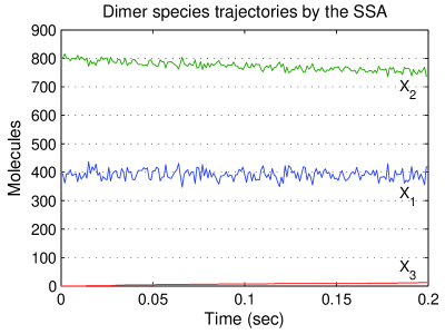
Figure 1: Time evolution of the numbers of molecules in the decaying-dimerizing problem (59). The simulation is carried out using Gillespie’s SSA method.

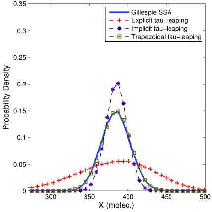
(a) Histograms obtained with Gillespie’s SSA, and with the traditional explicit, implicit, and trapezoidal tau-leaping methods.

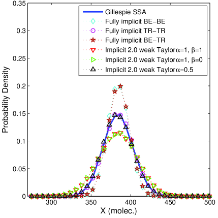
(b) Histograms obtained with Gillespie’s SSA, the new fully implicit methods, and the new implicit order two weak Taylor tau-leaping methods.

Figure 2: The histograms of the number of molecules $X_{1}$ at the final time for the decaying-dimerizing reaction system (59). All histograms are based on 100,000 runs of the corresponding methods with a fixed stepsize $\tau=2\times 10^{-4}$ seconds.

In order to compare the solutions given by different methods we consider histograms of $X_{1}$, the number of molecules of $S_{1}$, at the final time $T=0.2$ seconds. Specifically, an ensemble of simulation results is carried out for each method, and the final distribution of the numerical $X_{1}$ is plotted as a histogram from 100,000 independent simulations.

Figure 2(a) shows the histograms of $X_{1}$ for the decaying-dimerizing system (59) simulated with Gillespie’s SSA and with the traditional explicit tau-leaping, implicit tau-leaping, and trapezoidal tau-leaping methods. A fixed stepsize $\tau=2\times 10^{-4}$ seconds is used. Figure 2(b) also shows the histograms generated with Gillespie’s SSA, and with the methods proposed herein: fully implicit BE–BE, TR–TR, BE–TR, implicit order two weak Taylor with $\alpha=1.0$ and $\beta=1.0$, $\alpha=1.0$ and $\beta=0.0$, and $\alpha=0.5$. The same fixed stepsize $\tau=2\times 10^{-4}$ is used.

Figures 2 (a) and (b) reveal that the histograms of the trapezoidal tau-leaping method, fully implicit TR–TR method, and implicit order two weak Taylor method with $\alpha=0.5$ are closer to the reference (SSA) histogram than those of other methods, for the specific time step chosen.

The explicit method gives very unstable and varying results. Other implicit order two weak Taylor methods with $\alpha=1.0$ provoke a little wide varying results, but those escape the damping effect such as implicit tau-leaping method in Figure 2 (a). From the stability analysis, we have proved that the implicit order two weak Taylor methods with $\alpha=1.0$ are unstable for large stepsizes, and these experimental results confirm the conditional stability.

In order to numerically assess the accuracy of each method, we carry out simulations with different stepsizes, and obtain the corresponding histograms. For each method and step size the numerical errors are quantified by the difference between the numerical histograms and the reference (SSA) histogram. Two metrics of the difference are employed: the Kullback-Leibler (K-L) divergence [20] and the distance metric.

The K-L divergence is a non-commutative measure of the difference between two probability distributions $P$ and $Q$, typically $P$ representing the “true” distribution and $Q$ representing arbitrary probability distribution. Therefore we set $P$ to be the distribution obtained from SSA, and $Q$ the distribution obtained with one of the other formulae. The K-L divergence is defined to be

$$D_{KL}(P||Q)=\sum_{i}P(i)\log{P(i)\over Q(i)}$$ (60)

where $Q(i)\neq 0$, and the summation is taken over the histogram bins. Smaller values of K-L divergence represent more similar distributions. Because K-L divergence is not useful when there exists zeros for $Q$, we also use the distance metric, which measures the difference between two distributions by

$$Dist=\sum_{i}\Delta X\cdot|P(i)-Q(i)|\,.$$ (61)

Here $\Delta X$ is the bin size of the histogram.

Table 2: The mean, variance, K-L divergence, and distance for $X_{1}$ at $T=0.2$ based on 100,000 samples for different stepsizes of the decaying-dimerizing reaction system (59).

		Stepsize ($\tau$ in seconds)
Method	Metrics	$8\times 10^{-4}$	$4\times 10^{-4}$	$2\times 10^{-4}$	$1\times 10^{-4}$
Gillespie	Mean	387.19
SSA	Variance	349.87
Explicit	Mean	$\infty$	$\infty$	384.71	386.92
tau-leaping	Variance	$\infty$	$\infty$	2503.30	614.64
	K-L div.	$\infty$	$\infty$	0.740	0.092
	Distance	$\infty$	$\infty$	8.799	2.665
Implicit	Mean	387.95	387.86	387.92	387.81
tau-leaping	Variance	79.42	128.46	185.93	242.84
	K-L div.	0.329	0.176	0.080	0.030
	Distance	6.689	4.829	3.156	1.817
Trapezoidal	Mean	387.63	387.70	387.73	387.60
tau-leaping	Variance	351.29	346.61	346.38	347.24
	K-L div.	0.004	0.004	0.002	0.002
	Distance	0.617	0.584	0.444	0.370
Fully implicit	Mean	387.27	387.35	387.37	387.49
BE–BE	Variance	79.02	128.21	184.31	239.5
	K-L div.	0.329	0.174	0.080	0.031
	Distance	6.583	4.744	3.078	1.859
Fully implicit	Mean	387.26	387.43	387.51	387.61
TR–TR	Variance	348.09	343.71	344.10	346.91
	K-L div.	0.003	0.002	0.001	0.001
	Distance	0.413	0.312	0.296	0.276
Fully implicit	Mean	387.63	387.63	387.77	387.59
BE–TR	Variance	79.54	127.60	187.74	241.69
	K-L div.	0.326	0.177	0.077	0.030
	Distance	6.604	4.818	3.031	1.905
Implicit 2.0	Mean	$\infty$	$\infty$	386.49	387.12
weak Taylor	Variance	$\infty$	$\infty$	584.70	407.24
($\alpha=1,\beta=1$)	K-L div.	$\infty$	$\infty$	0.076	0.007
	Distance	$\infty$	$\infty$	2.426	0.672
Implicit 2.0	Mean	$\infty$	$\infty$	386.07	387.03
weak Taylor	Variance	$\infty$	$\infty$	591.80	409.78
($\alpha=1,\beta=0$)	K-L div.	$\infty$	$\infty$	0.080	0.007
	Distance	$\infty$	$\infty$	2.455	0.726
Implicit 2.0	Mean	387.29	387.26	386.44	386.25
weak Taylor	Variance	356.93	350.17	348.72	348.89
($\alpha=0.5$)	K-L div.	0.004	0.003	0.002	0.002
	Distance	0.625	0.421	0.386	0.318

Table 2 shows these metrics based on 100,000 samples generated by different methods for fixed stepsizes $\tau=(8/k)\times 10^{-4}$ where $k=1,2,4,8$. The results show that the mean is accurately computed by all accelerated methods. However, the variance and distance are different for each formula. For example, the explicit tau formula becomes very unstable for a stepsize of $4\times 10^{-4}$ seconds. The implicit tau-leaping, BE–BE, BE–TR are far superior to explicit tau, but those formulae produce smaller variances compared to the variance of the exact SSA that is called as damping effect.

Three methods (the trapezoidal-tau, the fully implicit TR–TR, and the implicit second order weak Taylor with $\alpha=0.5$) generate accurate variance results even with large stepsizes. The fully implicit TR–TR results are the most accurate among all methods for similar time steps, as demonstrated by the smaller distance to the reference histogram in Table 2. The implicit second order weak Taylor methods with $\alpha=1.0$ are accurate until they become unstable for large stepsizes.

Table 3: Elapsed CPU times (in seconds) for each method and time step for 100,000 simulations of the decaying-dimerizing reaction system (59).

CPU time (seconds)	Stepsize ($\tau$ in seconds)
Method	$8\times 10^{-4}$	$4\times 10^{-4}$	$2\times 10^{-4}$	$1\times 10^{-4}$
Gillespie SSA	16210.13
Explicit tau-leaping	27.32	46.91	130.55	260.24
Implicit tau-leaping	170.57	340.58	657.51	1389.29
Trapezoidal tau-leaping	180.42	350.66	688.98	1301.21
Fully implicit BE–BE	344.98	686.49	1395.1	2638.74
Fully implicit TR–TR	377.06	746.24	1400.96	2752.39
Fully implicit BE–TR	340.65	690.56	1373.31	2657.25
Implicit 2.0 weak Taylor ($\alpha=1,\beta=1$)	398.23	784.43	1587.69	3121.32
Implicit 2.0 weak Taylor ($\alpha=1,\beta=0$)	391.31	765.39	1532.98	3076.23
Implicit 2.0 weak Taylor ($\alpha=0.5$)	381.34	752.84	1425.83	2798.54

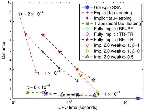
Figure 3: Relationship between solution accuracy (measured by the distance (61) between the accelerated method and the SSA produced histograms) and CPU time for different methods applied to the decaying-dimerizing reaction system (59).

The elapsed CPU times for each method are presented in Table 3. Figure 3 considers the relationship between accuracy and computation time for each of the accelerated methods. From the figure, the trapezoidal tau-leaping, the fully implicit TR–TR, and the implicit second order weak Taylor with $\alpha=0.5$ methods generate accurate solutions with a large step size ($\tau=8\times 10^{-4}$ seconds) and in a short CPU time. For comparison, 100,000 simulations using the SSA took 16,210 CPU seconds, while 100,000 simulations of the fully implicit TR–TR took only 377 seconds (2.3% of the SSA time) and provided an accurate solution (distance value is only 0.276). The implicit second order weak Taylor method of the $\alpha=0.5$ with $\tau=8\times 10^{-4}$ fixed step took 381 seconds and produced results of similar accuracy.

6.2 Schlögl Reaction Set

The Schlögl reaction model [15] is a simple but famous bistable system. The system contains four reactions

$$\begin{split}&B_{1}+2S\;\vbox{\offinterlineskip\hbox{$\displaystyle\buildrel c_{1}\over{\longrightarrow}$}\kern-1.0pt\hbox{$\displaystyle\mathrel{\mathop{\kern 0.0pt\longleftarrow}\limits_{c_{2}}}$}}\;3S,\\ &B_{2}\;\vbox{\offinterlineskip\hbox{$\displaystyle\buildrel c_{1}\over{\longrightarrow}$}\kern-1.0pt\hbox{$\displaystyle\mathrel{\mathop{\kern 0.0pt\longleftarrow}\limits_{c_{2}}}$}}\;S,\end{split}$$ (62)

where $B_{1}$ and $B_{2}$ are buffered species whose populations are assumed to remain constant over the time interval.

$$c_{1}=3\times 10^{-7},\quad c_{2}=10^{-4},\quad c_{3}=10^{-3},\quad c_{4}=3.5,N_{1}=1\times 10^{5},\quad N_{2}=2\times 10^{5}.$$

which will render the bistable system. Hence the propensity functions are given by

$$a_{1}=\frac{c_{1}}{2}N_{1}X(X-1),\quad a_{2}=\frac{c_{2}}{6}X(X-1)(X-2),\quad a_{3}=c_{3}N_{2},\quad a_{4}=c_{4}X$$

where $X$ denotes the number of molecules of species $S$. Initial condition $X(0)=250$ at $T=0$, and final time $T=4$ second.

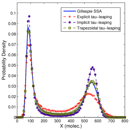
(a) Histograms obtained with Gillespie’s SSA, and with the traditional explicit, implicit, and trapezoidal tau-leaping methods.

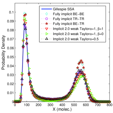
(b) Histograms obtained with Gillespie’s SSA, the new fully implicit methods, and the new implicit order two weak Taylor tau-leaping methods.

Figure 4: The histograms of the number of molecules $X$ at the final time for the Schlögl bistable system (62). All histograms are based on 100,000 runs of the corresponding methods with a fixed stepsize $\tau=0.4$ seconds.

The histograms generated from 100,000 independent samples of SSA, existing improved SSA methods, and proposed methods including fully implicit tau-leaping methods and implicit order two weak Taylor methods with fixed stepsize $\tau=0.4$ are shown in Figure 4. We notice that the histogram given by the trapezoidal tau-leaping method, fully implicit TR–TR method, and implicit order two weak Taylor method with $\alpha=0.5$ are very close to the exact SSA method than other methods for the specific time step as the histogram of the decaying-dimerizing system. The histograms produced by the fully implicit BE–BE and BE–TR exhibit damping effect (sharp peaks) while the histogram given by the implicit order two weak Taylor method with $\alpha=1.0$, $\beta=1.0$ and $\alpha=1.0$, $\beta=0.0$ methods provoke a little wide varying results (broad peaks).

Table 4: The mean, variance, distance, and elapsed CPU times (in seconds) for $X$ at $T=4$ based on 100,000 samples for different stepsizes of the Schlögl bistable system (62).

		Stepsize ($\tau$ in seconds)
Method	Metrics	$0.8$	$0.4$	$0.2$	$0.1$
Gillespie	Mean (Var)	305.2 (46465.9)
SSA	CPU time	682.96
Explicit	Mean (Var)	296.9 (40957.6)	306.2 (42915.6)	309.5 (44981.5)	308.5 (45929.9)
tau-leaping	Distance	5.680	3.155	2.057	1.860
	CPU time	1.41	2.1	3.43	6.21
Implicit	Mean (Var)	343.4 (52245.0)	326.3 (49876.8)	316.9 (48364.8)	315.1 (47644.7)
tau-leaping	Distance	4.464	2.877	2.136	1.936
	CPU time	4.41	7.03	12.24	22.4
Trapezoidal	Mean (Var)	324.6 (47837.6)	317.4 (47161.6)	312.6 (46727.0)	311.2 (46719.1)
tau-leaping	Distance	2.036	1.906	1.849	1.818
	CPU time	4.2	6.79	12.07	22.6
Fully implicit	Mean (Var)	316.4 (51137.7)	318.8 (49359.6)	313.5 (47919.2)	312.2 (47401.1)
BE–BE	Distance	4.360	2.808	2.158	1.956
	CPU time	8.64	13.6	23.74	43.86
Fully implicit	Mean (Var)	316.2 (47195.7)	312.4 (46743.9)	312.2 (46624.0)	309.9 (46601.9)
TR–TR	Distance	1.943	1.857	1.836	1.818
	CPU time	8.13	13.63	24.51	46.4
Fully implicit	Mean (Var)	335.5 (51920.4)	322.3 (49566.8)	315.9 (48011.9)	311.1 (47325.1)
BE–TR	Distance	4.417	2.761	2.147	1.917
	CPU time	8.80	13.38	24.98	46.76
Implicit 2.0	Mean (Var)	1122.4 (51112.5)	310.3 (49157.7)	310.2 (47332.8)	310.0 (46612.9)
weak Taylor	Distance	3.501	1.890	1.830	1.766
($\alpha=1,\beta=1$)	CPU time	12.53	18.72	30.98	55.08
Implicit 2.0	Mean (Var)	296.4 (50810.1)	306.2 (46870.6)	309.5 (46566.0)	309.7 (46498.5)
weak Taylor	Distance	2.475	1.869	1.842	1.839
($\alpha=1,\beta=0$)	CPU time	11.74	17.48	28.76	52.64
Implicit 2.0	Mean (Var)	313.2 (47441.4)	309.9 (46880.3)	309.7 (46494.3)	310.2 (46503.7)
weak Taylor	Distance	1.862	1.840	1.809	1.803
($\alpha=0.5$)	CPU time	10.71	16.34	26.47	50.23

Table 4 shows the mean, variance, distance, and elapsed CPU times based on 100,000 samples generated by different methods for fixed stepsizes. Four fixed stepsizes $\tau=0.8/k$ where $k=1,2,4,8$ were selected to evaluate accuracy for each time step. The variance for all methods are large for the bistability property of the system. Proposed fully implicit TR–TR, and the implicit second order weak Taylor with $\alpha=0.5$ produce accurate results even with large stepsize $\tau=0.8$.

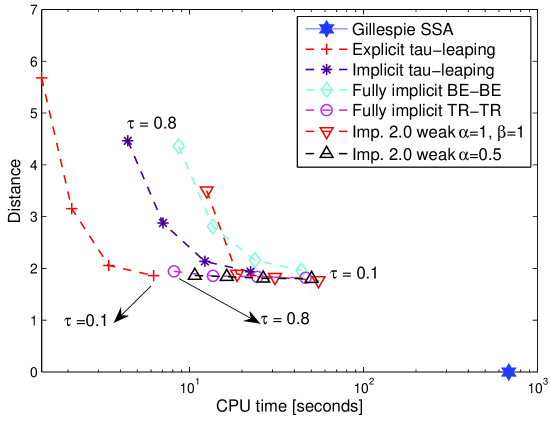
Figure 5: Relationship between solution accuracy measured by the distribution distance (61) and CPU time for different methods applied to the Schlögl bistable system (62).

Figure 5 shows the relationship between distance of two distributions (the SSA and each accelerated method distributions) and computation time for the different stepsizes of Schlögl bistable system. As the previous dimer reaction system, the fully implicit TR–TR and the implicit second order weak Taylor method with the $\alpha=0.5$ show small distance (good accuracy) compared to other accelerated methods with the big stepsize $\tau=0.8$. 100,000 simulations of the fully implicit TR–TR method with the $\tau=0.8$ took 8.13 seconds with accuracy. With the limited results investigated here, the explicit tau-leaping method is the most efficient for this system. 100,000 simulations of the explicit tau-leaping method for the small stepsize $\tau=0.1$ took 6.21 seconds with small distance as ones of fully implicit TR–TR results for the stepsize $\tau=0.4$. All accelerated methods show efficiency (at least 10 times faster) compared to the SSA that took 683 seconds for 100,000 simulations.

6.3 The ELF System

We now consider a more complex system containing 8 species and 12 reactions [21, 22, 13] to evaluate the accuracy of the proposed tau-leaping methods. We use the initial conditions and parameter values given in the literature [13]. The chemical reactions, propensity functions, and initial values are listed in Table 5.

Table 5: List of reactions and propensity functions for the ELF system.

	Reaction	Propensity	Rate constant		Species	Initial value
$R_{1}$	$E_{A}\rightarrow E_{A}+A$	$a_{1}=c_{1}[E_{A}]$	$c_{1}=15$	$X_{1}$	$A$	2000 molec.
$R_{2}$	$E_{B}\rightarrow E_{B}+B$	$a_{2}=c_{2}[E_{B}]$	$c_{2}=15$	$X_{2}$	$B$	1500 molec.
$R_{3}$	$E_{A}+B\rightarrow E_{A}B$	$a_{3}=c_{3}[E_{A}][B]$	$c_{3}=0.0001$	$X_{3}$	$E_{A}$	950 molec.
$R_{4}$	$E_{A}B\rightarrow E_{A}+B$	$a_{4}=c_{4}[E_{A}B]$	$c_{4}=0.6$	$X_{4}$	$E_{B}$	950 molec.
$R_{5}$	$E_{A}B+B\rightarrow E_{A}B_{2}$	$a_{5}=c_{5}[E_{A}B][B]$	$c_{5}=0.0001$	$X_{5}$	$E_{A}B$	200 molec.
$R_{6}$	$E_{A}B_{2}\rightarrow E_{A}B+B$	$a_{6}=c_{6}[E_{A}B_{2}]$	$c_{6}=0.6$	$X_{6}$	$E_{A}B_{2}$	50 molec.
$R_{7}$	$A\rightarrow 0$	$a_{7}=c_{7}[A]$	$c_{7}=0.5$	$X_{7}$	$E_{B}A$	200 molec.
$R_{8}$	$E_{B}+A\rightarrow E_{B}A$	$a_{8}=c_{8}[E_{B}][A]$	$c_{8}=0.0001$	$X_{8}$	$E_{B}A_{2}$	50 molec.
$R_{9}$	$E_{B}A\rightarrow E_{B}+A$	$a_{9}=c_{9}[E_{B}A]$	$c_{9}=0.6$
$R_{10}$	$E_{B}A+A\rightarrow E_{B}A_{2}$	$a_{1}0=c_{1}0[E_{B}A][A]$	$c_{1}0=0.0001$
$R_{11}$	$E_{B}A_{2}\rightarrow E_{B}A+A$	$a_{1}1=c_{1}1[E_{B}A_{2}]$	$c_{1}1=0.6$
$R_{12}$	$B\rightarrow 0$	$a_{1}2=c_{1}2[B]$	$c_{1}2=0.5$

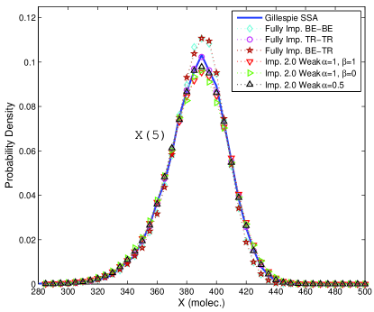
(a) $~{}~{}\tau=0.04$ sec.

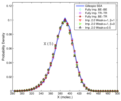
(b) $~{}~{}\tau=0.005$ sec.

Figure 6: The histograms of $X_{5}$ at the final time obtained with different, fixed stepsizes for the ELF system (Table 5). Each histogram uses 100,000 samples.

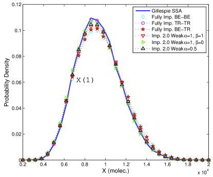
(a) $~{}~{}\tau=0.04$ sec.

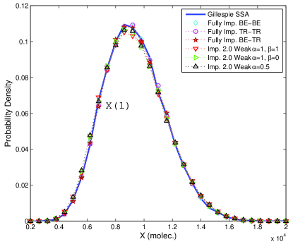
(b) $~{}~{}\tau=0.005$ sec.

Figure 7: The histograms of $X_{1}$ at the final time obtained with different, fixed stepsizes for the ELF system (Table 5). Each histogram uses 100,000 samples.

We consider the simulation time interval $[0,3]$ seconds, and perform 100,000 independent runs with the Gillespie SSA and with each one of the accelerated methods. The histograms of $X_{5}$ and $X_{1}$ concentrations at the final time are presented in Figures 6 and 7, respectively, for different fixed time steps between $\tau=0.04$ and $\tau=0.005$ seconds. Figure 6 shows a similar qualitative behavior as in the previous stiff examples. For a large stepsize $\tau=0.04$ seconds, the histograms produced by the fully implicit BE–BE and BE–TR methods exhibit a weak damping effect (small sharp peaks), while the histograms given by the implicit order two weak Taylor methods with $\alpha=1.0$ exhibit a dispersive effect (broader peaks). Figure 7 shows a different behavior. For a large stepsize $\tau=0.04$ seconds the BE–BE, the BE–TR, and the implicit order 2.0 weak Taylor with $\alpha=1.0$ methods show dispersive behavior (broad peaks). Therefore the errors in variance for the ELF system have a complex behavior when stepsizes are very large. In Figures 6 and 7, the histograms given by the fully implicit TR–TR method and implicit order two weak Taylor method with $\alpha=0.5$ are very similar to the exact SSA histogram. If the stepsize $\tau$ is decreased to $\tau=0.005$ seconds, all approximation methods show very good accuracy.

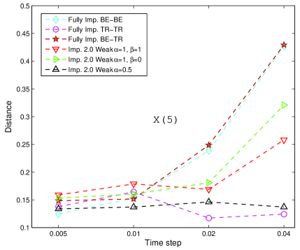
(a) Error in the distribution of $X_{5}$.

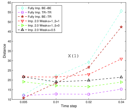
(b) Error in the distribution of $X_{1}$.

Figure 8: The relationship between the error in distribution (the distance (61) between SSA and each of the proposed methods’ histograms) and the different stepsizes for $X_{5}$ and $X_{1}$ for the ELF system.

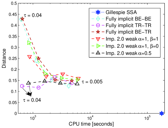
Figure 9: The relationship between accuracy and CPU time for $X_{5}$ of the ELF system

Figures 8 (a) and (b) show the error in distribution (the distance (61) between the SSA and each of the accelerated methods’ histograms) versus simulation stepsize for the ELF system. The y-scale in Figure 8 (b) is much larger than that of Figure 8 (a) because the number of molecules for $X_{1}$ is much larger than that of $X_{5}$ (see the Figures 6 and 7). The results indicate that, similar to the previous examples, the TR–TR and the implicit second order weak Taylor method with the $\alpha=0.5$ are the most accurate accelerated methods.

Figure 9 shows the relationship between accuracy and CPU time for the different stepsizes of the ELF system. The accuracy is measured by the distance (61) between the accelerated method and the SSA histograms for $X_{5}$, as in Figure 8 (a). 100,000 simulation of the SSA took 178,364 seconds (approximately 50 hours), while 100,000 simulations of the implicit order two weak Taylor method with $\alpha=1.0$ and $\beta=1.0$ for the smallest stepsize $\tau=0.005$ took 6,216 seconds (3.5% of the SSA time) and provided an accurate solution (distance value is only 0.15). For the largest fixed stepsize $\tau=0.04$ seconds, the fully implicit TR–TR and the implicit second order weak Taylor method with the $\alpha=0.5$ provide high accuracy and high efficiency (only 0.4% of the SSA time).

7 Conclusions

This paper develops new implicit tau-leaping-like algorithms for the solution of stochastic chemical kinetic systems. The fully implicit tau-leaping methods, “BE–BE”, “TR–TR”, and “BE–TR”, are motivated by the fact that existing implicit tau-leaping algorithms treat implicitly only the mean part of the Poisson process. The newly proposed methods treat implicitly the variance of the Poisson variables as well. The implicit second order weak Taylor tau-leaping methods are motivated by the theory of weakly convergent discretizations of stochastic differential equations, and by the fact that Poisson variables with large mean are well approximated by normal variables.

Theoretical stability and consistency analyses are carried out on a standard test problem – the reversible isomerization reaction. The fully implicit tau-leaping methods are unconditionally stable; the implicit second order weak Taylor tau-leaping methods with $\alpha=1.0$ are conditionally stable, and with $\alpha=0.5$ unconditionally stable. The asymptotic means of the solutions given by all proposed methods converge to the analytical mean of the test problem. The asymptotic variances of the proposed methods, however, converge to different values, as it is also the case for traditional tau-leaping methods.

Numerical experiments are carried out using the decaying-dimerizing system, the bistable Schlögl reaction system, and the ELF system to validate the theoretical results. The accuracy of the solutions is evaluated by comparing the probability densities obtained with the new methods and with Gillespie’s SSA. The numerical results verify that the prosed methods are accurate, with an efficiency comparable to that of the traditional implicit tau-leaping methods. The theoretical analyses and numerical experiments shows that the fully implicit TR–TR and the implicit second order weak Taylor tau-leaping methods with $\alpha=0.5$ are the most accurate methods for large stepsizes.

References

- [1] H. H. McAdams, A. Arkin, Stochastic mechanisms in gene expression, Proc. Natl. Acad. Sci. 94 (3) (1997) 814–819.
- [2] D. T. Gillespie, A rigorous derivation of the chemical master equation, Physica A 188 (1–3) (1992) 404–425.
- [3] N. G. van Kampen, Stochastic Processes in Physics and Chemistry, North Holland, North Holland, Netherlands.
- [4] D. T. Gillespie, Exact stochastic simulation of coupled chemical reactions, Journal of Physical Chemistry 81 (25) (1977) 2340–2361.
- [5] D. T. Gillespie, Approximate accelerated stochastic simulation of chemically reacting systems, Journal of Chemical Physics 115 (4) (2001) 1716–1733.
- [6] M. Rathinam, L. R. Petzold, Y. Cao, D. T. Gillespie, Stiffness in stochastic chemically reacting systems: The implicit tau-leaping method, Journal of Chemical Physics 119 (24) (2003) 12784–12794.
- [7] Y. Cao, L. Petzold, Trapezoidal tau-leaping formula for the stochastic simulation of biochemical systems, in: Proceedings of Foundations of Systems Biology in Engineering (FOSBE 2005), 2005, pp. 149–152.
- [8] Y. Cao, H. Li, L. Petzold, Efficient formulation of the stochastic simulation algorithm for chemically reacting systems, Journal of Chemical Physics 121 (9) (2004) 4059–4067.
- [9] D. T. Gillespie, L. R. Petzold, Improved leap-size selection for accelerated stochastic simulation, Journal of Chemical Physics 119 (16) (2003) 8229–8234.
- [10] M. Rathinam, L. R. Petzold, Y. Cao, D. T. Gillespie, Consistency and stability of tau leaping schemes for chemical reaction systems, SIAM Journal of Multiscale Modeling and Simulation 4 (3) (2005) 867–895.
- [11] T. Tian, K. Burrage, Implicit taylor methods for stiff stochastic differential equations, Applied Numerical Mathematics 38 (1-2) (2001) 167–185.
- [12] T. Li, Analysis of explicit tau-leaping schemes for simulating chemically reacting systems, Multiscale Modeling and Simulation 6 (2) (2007) 417–436.
- [13] Y. Hu, T. Li, B. Min, A weak second order tau-leaping method for chemical kinetic systems, Journal of Chemical Physics 135 (2) (2011) 024113.
- [14] P. E. Kloeden, E. Platen, Numerical Solution of Stochastic Differential Equations, Springer, New York, NY.
- [15] Y. Cao, L. R. Petzold, M. Rathinam, D. T. Gillespie, The numerical stability of leaping methods for stochastic simulation of chemically reacting systems, Journal of Chemical Physics 121 (24) (2004) 12169–12178.
- [16] T.-H. Ahn, A. Sandu, Fully implicit tau-leaping methods for the stochastic simulation of chemical kinetics, in: Proceedings of the 2011 Spring Simulation Multiconference, SpringSim ’11, Society for Computer Simulation International, Boston, MA, USA, 2011.
- [17] T.-H. Ahn, A. Sandu, Implicit second order weak taylor tau-leaping methods for the stochastic simulation of chemical kinetics, Vol. 4, 2011, pp. 2297 – 2306, proceedings of the International Conference on Computational Science, ICCS 2011.
- [18] I. I. Gikhman, A. V. Skorokhod, Stochastic Differential Equations, Springer, New York, NY, 1972.
- [19] S. M. Ross, Introduction to Probability Models, Ninth Edition, Academic Press, Inc., Orlando, FL, USA, 2006.
- [20] F. Emmert-Streib, M. Dehmer, Information Theory and Statistical Learning, Springer, New York, NY, 2008.
- [21] J. Elf, M. Ehrenberg, Spontaneous separation of bi-stable biochemical systems into spatial domains of opposite phases, Systems Biology, IEE Proceedings 1 (2) (2004) 230 – 236.
- [22] T. T. Marquez-Lago, K. Burrage, Binomial tau-leap spatial stochastic simulation algorithm for applications in chemical kinetics, Journal of Chemical Physics 127 (10) (2007) 104101.