Improving the precision of time-delay cosmography with observations of galaxies along the line of sight

Abstract

In order to use strong gravitational lens time delays to measure precise and accurate cosmological parameters the effects of mass along the line of sight must be taken into account. We present a method to achieve this by constraining the probability distribution function of the effective line of sight convergence $\kappa_{\rm ext}$. The method is based on matching the observed overdensity in the weighted number of galaxies to that found in mock catalogs with $\kappa_{\rm ext}$ obtained by ray-tracing through structure formation simulations. We explore weighting schemes based on projected distance, mass, luminosity, and redshift. This additional information reduces the uncertainty of $\kappa_{\rm ext}$ from $\sigma_{\kappa}\sim$0.06 to $\sim$0.04 for very overdense lines of sight like that of the system B1608$+$656. For more common lines of sight, $\sigma_{\kappa}$ is reduced to $\lesssim$0.03, corresponding to an uncertainty of $\lesssim 3$% on distance. This uncertainty has comparable effects on cosmological parameters to that arising from the mass model of the deflector and its immediate environment. Photometric redshifts based on g, r, i and K photometries are sufficient to constrain $\kappa_{\rm ext}$ almost as well as with spectroscopic redshifts. As an illustration, we apply our method to the system B1608$+$656. Our most reliable $\kappa_{\rm ext}$ estimator gives $\sigma_{\kappa}$=0.047 down from 0.065 using only galaxy counts. Although deeper multi-band observations of the field of B1608$+$656 are necessary to obtain a more precise estimate, we conclude that griK photometry, in addition to spectroscopy to characterize the immediate environment, is an effective way to increase the precision of time-delay cosmography.

1. INTRODUCTION

Strong gravitational lensing can be used to study a number of important astrophysical topics, ranging from the mass distribution within galaxies (e.g., Kochanek, 1991; Treu & Koopmans, 2002) and clusters of galaxies (e.g., Kneib et al., 1993; Limousin et al., 2007; Sand et al., 2008) to magnifying distant sources (e.g., Pettini et al., 2000; Ellis et al., 2001; Richard et al., 2008), to cosmography (e.g., Kochanek, 1996; Schechter et al., 1997; Oguri, 2007) (see recent reviews by Courbin et al., 2002; Meylan et al., 2006; Treu, 2010; Bartelmann, 2010; Kneib & Natarajan, 2011, for extensive references).

The power of lensing as a tool for astrophysics stems from its ability to measure mass independent of its dynamical state, as well as from its ability to magnify background sources. Detailed mass models of the deflector galaxies, groups, or clusters of galaxies can be determined by reproducing the strong lensing observables, i.e. multiple image time delays, positions, and fluxes (e.g., Keeton, 2010, and references therein). However, one of the main limitations of gravitational lensing is due to the so-called “mass-sheet degeneracy” (Falco et al., 1985; Schneider & Seitz, 1995; Saha, 2000; Wucknitz, 2002). This emerges from considering the solution to the lens equation, characterized by a certain surface mass density $\kappa$ for the deflector in units of the critical density $\Sigma_{\rm crit}$. By linear transformations, one finds that an infinite family of solutions can be obtained. The family of solutions results in a range of inferred properties both for the mass model of the main deflector as well as for the properties of the lensed source. One needs to break the mass-sheet degeneracy using physical arguments in order to fully exploit the power of gravitational lensing.

A number of strategies have been adopted to break this degeneracy both in the strong and weak lensing regimes (e.g., Broadhurst et al., 1995; Kneib et al., 2003; Bradač et al., 2004; Sonnenfeld et al., 2011). A common strategy is requiring the surface mass density of the main deflector to vanish at large distances from its center. This solution is physically equivalent to assuming that the distribution of mass along the line of sight (LOS), excluding the plane of the main deflector, is uniform and equal to the average of the Universe. This approximation is sufficient for many applications of gravitational lensing, resulting typically in uncertainties of only a few percent in the inferred mass distribution of the main deflector and in the luminosity and size of the lensed source (Seljak, 1994; Keeton et al., 1997; Koopmans et al., 2006; Treu et al., 2009; Hoekstra et al., 2011). For higher precision measurements however, one needs to determine the effects of the line of sight mass distribution. It is customary to condense these effects into an equivalent additional mass sheet at the redshift of the main deflector with uniform surface mass density $\kappa_{\rm ext}$, which can be positive or negative depending on whether the line of sight is over or underdense with respect to the average of the Universe (Schneider, 1997). In practice, mass-sheet degeneracy can be broken, i.e., the value of $\kappa_{\rm ext}$ can be inferred, by constraining in an independent way (1) the mass of the lens galaxy via stellar kinematics (e.g., Treu & Koopmans, 2002; Koopmans & Treu, 2003; Barnabè et al., 2009; Auger et al., 2010; Suyu et al., 2010; Sonnenfeld et al., 2012), and/or (2) the total mass of any intervening mass structures along the line of sight via imaging and spectroscopy of objects along the line of sight (e.g., Keeton & Zabludoff, 2004; Fassnacht et al., 2006; Momcheva et al., 2006; Suyu et al., 2010; Wong et al., 2011; Fassnacht et al., 2011).

Determining $\kappa_{\rm ext}$ is especially important for doing precision cosmography with gravitational lens time delays. Gravitational lens time delays are the difference in the arrival time of photons along the paths corresponding to multiple images arising from geometric and general relativistic effects. For variable sources, like active galactic nuclei, time delays can be measured via dedicated monitoring campaigns (e.g., Fassnacht et al., 2002; Fohlmeister et al., 2008; Paraficz et al., 2009; Courbin et al., 2011; Tewes et al., 2012). If the mass distribution in the plane of the deflector and along the line of sight is known, the measured time delays can be converted to the so-called time-delay distance $D_{\Delta t}$, a combination of three angular diameter distances (e.g., Treu, 2010). In turn, the time-delay distance contains information on cosmological parameters, primarily the Hubble constant $H_{0}$ (Refsdal, 1964), but also the curvature and other parameters (Coe & Moustakas, 2009; Suyu et al., 2010; Linder, 2011). To first approximation, time delays constrain cosmology in a similar way to baryon acoustic oscillation experiments and therefore are an excellent complement to other probes like the cosmic microwave background and type Ia Supernovae (Linder, 2011; Das & Linder, 2012). It has been shown that with current techniques and sufficient ancillary data a single gravitational lens measures the time-delay distance to approximately $5$-$6$% (Suyu et al., 2010, 2013).

In cases like B1608$+$656 where the time delays are known to $\sim$2% and the mass model of the main deflector and its immediate environment is exquisitely constrained by the data, the dominant source of uncertainty is the distribution of mass along the line of sight (e.g., Bar-Kana, 1996), i.e. effectively the external convergence $\kappa_{\rm ext}$. Specifically, $D_{\Delta t}\propto(1-\kappa_{\rm ext})^{-1}$. Thus, for small $\kappa_{\rm ext}$, the uncertainty $\sigma_{\kappa}$ translates directly into relative uncertainty in time-delay distance, currently dominating the overall error budget.

Suyu et al. (2010) constrained $\kappa_{\rm ext}$ by using the density of galaxies within $45^{\prime\prime}$ of B1608$+$656, which was measured to be twice that of an average field observed at the same depth by Fassnacht et al. (2011). Then, by selecting lines of sight with the same galaxy overdensity $\zeta_{\rm gal}$ in the Millennium ray-tracing simulations of Hilbert et al. (2009), they measured the conditional probability distribution function (PDF), $P(\kappa_{\rm ext}|\zeta_{\rm gal})$, which was then used as a prior in deriving cosmological information. Several efforts are underway to explore ways to further reduce this source of uncertainty. Those include spectroscopic and photometric surveys (Momcheva et al., 2006; Williams et al., 2008; Auger et al., 2007) as well as measurements of the external shear (Suyu et al., 2013)

In this paper we focus on refining and developing practical tools to estimate external convergence by comparing the output of cosmological numerical simulations with readily available observables such as those that can be derived from a galaxy photometric catalog. We define the relative overdensity $\zeta$ as the value of selected observables related to the stellar mass, the redshift, and the projected distance on the sky (angular distance) divided by the mean of the same observables over all lines of sight. Extending the work of Suyu et al. (2010) we consider a set of observables with relative overdensities $\zeta$ in addition to $\zeta_{\rm gal}$, the number of galaxies along a LOS divided by the average, seeking observables that minimize $\sigma_{\kappa}$. In a companion paper, Collett et al. (2013, submitted) a halo-model approach is used to perform a full reconstruction of the mass distribution along the line of sight, and thus provide a theoretical counterpart to the methods and weighting schemes developed here.

The main result of this paper is that using these statistics it is possible to reduce significantly $\sigma_{\kappa}$, using a multiband photometric catalog. The amount of gain depends on the specific line of sight, but for a system like B1608+656 it is possible to reduce it from 6 to 5% (even 4% in the best cases). We note that even reducing the uncertainty on a single lens from 5 to 4% is extremely useful given how rare these strong lenses are and how time-consuming it is to obtain ancillary data like time delays and high-resolution images. Oversimplifying for the purpose of illustration, assuming a target precision of 1% from a sample of lenses, only 16 systems would be needed if each were precise to 4%, as opposed to 25 systems at 5% precision each.

The paper is organized as follows. In Section 2 we briefly summarize the Millennium Simulation that forms the backbone of our study. In Section 3 we revisit the galaxy count statistic $\zeta_{\rm gal}$. In Section 4 we introduce other statistics involving stellar mass, luminosity, redshift, and distance. In Section 5 we test the influence of using photometric redshifts instead of spectroscopic redshifts in our method. In Section 6 we apply our method for several statistics to the gravitational lens B1608$+$656. Throughout the paper magnitudes are given on the Vega scale.

2. SUMMARY OF THE MILLENNIUM SIMULATION

Numerical simulations of large-scale structure provide a way to determine statistically the amount of external convergence for a lens system. By ray tracing through the Millennium Simulation (Springel et al., 2005), one can produce a simulated image of the sky populated with galaxies and a corresponding map of the external convergence, $\kappa_{\rm ext}$, for a given source redshift (Hilbert et al., 2007, 2008, 2009). The distribution of $\kappa_{\rm ext}$ values associated with lines of sight in the simulation that resemble the lens system of interest (e.g., in terms of the overdensity of galaxies around the lens system) provides a statistical estimate of the $\kappa_{\rm ext}$ for the lens system.

We use 64 simulated fields of $4\times 4$ deg² from the Millennium Simulation containing galaxies with positions, redshifts, magnitudes (in SDSS u,g,r,i,z and 2MASS J,H,K) and stellar masses from the semianalytic galaxy model of Guo et al. (2011). Each field has approximately 5 million galaxies with redshifts up to $\sim 3.2$ and an associated map of the external convergence on a $4096\times 4096$ grid for a source redshift of 1.4, typical of strong lensing systems like B1608$+$656. We use each position on the $\kappa_{\rm ext}$ map as a line of sight, and therefore have approximately $10^{9}$ lines of sight for the 64 fields. Hilbert et al. (2009) and Suyu et al. (2010) showed that the distribution of $\kappa_{\rm ext}$ from strong lens lines of sight are very similar to the distribution for all lines of sight. Therefore, we consider all lines of sight from the 64 fields in our analysis. These lines of sight provide the pool from which we select subsets that have observational properties (based on the galaxies) matching those of the lens system for determining the $\kappa_{\rm ext}$ of the lens.

3. GALAXY NUMBER COUNTS AS A PROBE OF $\kappa_{\rm ext}$

In this section we revisit the galaxy overdensity statistic introduced by Suyu et al. (2010). We recall that the use of relative overdensities – instead of absolute densities – in both the data and simulations is meant to minimize the impact of theoretical and observational systematic uncertainties. In particular this should reduce sensitivity to the choice of a specific reference simulation (Suyu et al., 2010).

In practice, we study $P(\kappa_{\rm ext}|\zeta_{\rm gal})$, where $\zeta_{\rm gal}$ is given by the number of galaxies within $45^{\prime\prime}$, $N_{\rm gal}$, in a specific line of sight, divided by the average value for all lines of sight, $\overline{N_{\rm gal}}$; i.e. $\zeta_{\rm gal}\equiv\frac{N_{\rm gal}}{\overline{N_{\rm gal}}}$. For the Millennium Simulation data, $\overline{N_{\rm gal}}$ is readily computed by multiplying the total number of galaxies by $\pi r^{2}/A$ where $r=45^{\prime\prime}$ and $A$ is the angular area of the entire field. However, in practice one must be careful of masked regions and edge effects. The choice of the radius is motivated by practical reasons. As discussed by Fassnacht et al. (2011), this is typically the maximum radius that can be surveyed for a target in middle of one of the two chips, i.e. the standard pointing of the Wide Field Camera of the Advanced Camera for Surveys (ACS) on board the Hubble Space Telescope (HST). We also impose restrictions similar to observations of B1608$+$656 such that all galaxies must have $0<z<z_{\rm source}$ (where $z_{\rm source}=1.394$ is the source redshift of B1608$+$656, Fassnacht et al., 1996), and following Fassnacht et al. (2011), have $18.5<{\rm mag_{i}}<24.5$. The results found by Suyu et al. (2010) used only the latter constraint. In Section 6, we revisit this field with redshift information. Once the PDFs of $\kappa_{\rm ext}$ are computed we define the width of the PDF $\sigma_{\kappa}$ as the semidifference of the 84 and 16 percentiles of $P(\kappa_{\rm ext}|\zeta_{\rm gal})$. We remind the reader that in this paper we use the convergence maps detailed in Section 2 to supply our $\kappa_{\rm ext}$ values.

The $\kappa_{\rm ext}$ PDF for a LOS with a known relative overdensity in galaxy count is readily computed by first counting $N_{\rm gal}$ for each line of sight on the convergence maps. The convergence maps are defined on a regular grid with resolution of $\sim$3.5^′′, and the grid points thus conveniently serve as locations of the lines of sight for our galaxy number counts. Then, it is sufficient to select lines of sight with overdensity close to the desired value $\zeta_{\rm gal}$. In practice, we select all lines of sight with

$$\left\lvert N_{\rm gal}-\zeta_{\rm gal}\overline{N_{\rm gal}}\right\rvert<E$$ (1)

where $E$, the interval width, is some integer value. As we increase $E$, the number of lines of sight satisfying Equation (1) also increases. As a general rule the parameter $E$ should be chosen to be as small as possible while still leaving sufficient lines of sight to generate the PDF. Note that sample variance noise is already introduced by the simulations so we expect that varying $E$ while keeping it smaller than $\sim\sqrt{N_{\rm gal}}$ should not affect our results.

A number of subtleties must be taken into account when constructing the $\kappa_{\rm ext}$ PDFs. As expected, the distributions are in general highly skewed. For example, fewer lines of sight become available at higher relative overdensities (and similarly at lower underdensities; for conciseness we shall discuss explicitly only the overdensities in our examples). Because the number of lines of sight $N_{\rm LOS}$ at a given galaxy count $N_{\rm gal}$ are always greater than that at $N_{\rm gal}+1$, simply constructing a PDF from all $\kappa_{\rm ext}$ whose corresponding $N_{\rm gal}$ satisfy Equation (1) would be biased towards lower $N_{\rm gal}$, and their respective $\kappa_{\rm ext}$ values. We define $\kappa_{\rm ext}^{\rm med}$ as the median $\kappa_{\rm ext}$ for a given PDF, and find that a good indicator of the bias in a sample is the change in $\kappa_{\rm ext}^{\rm med}$ as function of the interval width $E$. The narrowest interval $E=1$ gives the closest estimate to the true median. Since lower $N_{\rm gal}$ pull the entire PDF away from that with a galaxy count of $\zeta_{\rm gal}\overline{N_{\rm gal}}$, we expect that a notable change in $\kappa_{\rm ext}^{\rm med}$ will occur when we increase $E$. This is shown in the top panel of Figure 1. To circumvent this shift in $\kappa_{\rm ext}^{\rm med}$ that would lead to a bias in the time-delay distance determination, we weight each value of $\kappa_{\rm ext}$ by $\frac{1}{N_{\rm LOS}}$ for its respective $N_{\rm gal}$ – that is, we find $N_{\rm LOS}$ for the $N_{\rm gal}$ responsible for contributing a particular $\kappa_{\rm ext}$, and multiply by the inverse. Therefore each of the $2E$ $\kappa_{\rm ext}$ PDFs for a given $N_{\rm gal}$ within $\zeta_{\rm gal}\overline{N_{\rm gal}}\pm E$ carries equal weight, and $\kappa_{\rm ext}$ from higher $N_{\rm gal}$ offset those from lower, thus ensuring that our overall distribution remains relatively static. This is indeed the case, as the bottom panel of Figure 1 shows $\kappa_{\rm ext}^{\rm med}$ declines much more slowly as a function of uncertainty than in the upper panel.

However, maintaining a steady median has resulted in increasing the width of the distribution $\sigma_{\kappa}$. This is expected because PDFs on either side of $\zeta_{\rm gal}\overline{N_{\rm gal}}$ are centered slightly above or below our target. For this reason – and that of residual effects on the median – we see that lower galaxy interval widths ($E$) offer the best results, assuming they can encompass sufficient data to adequately reduce statistical uncertainty. For the purposes of this paper unless otherwise noted we set $E=2$.

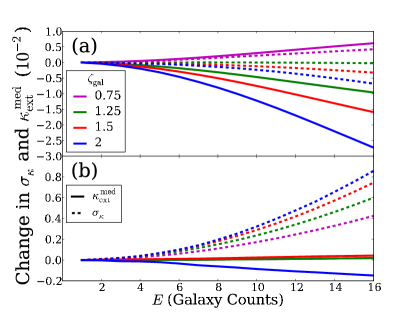
Figure 1.— Change in $\kappa_{\rm ext}^{\rm med}$ (solid) and $\sigma_{\kappa}$ (dashed) with $E$ for $\zeta_{\rm gal}=0.75,1.25,1.5$, and $2$ as measured from numerical simulations. The change is computed for both (a) unweighted and (b) weighted PDF combination, by subtracting $\kappa_{\rm ext}^{\rm med}$ and $\sigma_{\kappa}$ for the given distribution at $E$ by those at $E=1$. Unweighted refers to simply averaging $\kappa_{\rm ext}$ values for all LOS that satisfy (1), whereas weighted indicates weighting inversely by the number of LOS of a particular galaxy count. The $\kappa_{\rm ext}^{\rm med}$ line for $\zeta_{\rm gal}=0.75$ in panel (b) follows a nearly identical line to that of 1.25 and therefore is barely visible.

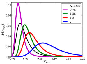
Figure 2.— PDFs for $\kappa_{\rm ext}$ constructed from lines of sight that satisfy Equation (1) for $\zeta_{\rm gal}=0.75,1.25,1.5$, and $2$ and $E=2$ as measured from numerical simulations.

As an illustration of our method, in this paper we investigate the underdense case $\zeta_{\rm gal}=0.75$ and the overdense cases $\zeta_{\rm gal}=1.25,1.5$, and $2$ (used in Figure 1), although our method carries over to any arbitrary value of $\zeta_{\rm gal}$. We show in Figure 2 the PDF of $\kappa_{\rm ext}$ for these $\zeta_{\rm gal}$ values. As expected, larger $\zeta_{\rm gal}$ produces a shift in the PDF along positive $\kappa_{\rm ext}$, however, it also increases $\sigma_{\kappa}$. In other words more overdense lines of sight have higher convergence but also a broader range of possible convergences. In the study of Fassnacht et al. (2011), B1608$+$656 possessed a relative overdensity of 2.18 without redshift cuts. We will thus look at the case of $\zeta_{\rm gal}=2$ with particular interest.

4. ALTERNATE CHARACTERISTICS AS WEIGHTS

Defining $\zeta_{\rm gal}=N_{\rm gal}/\overline{N_{\rm gal}}$ is useful for constructing PDFs of $\kappa_{\rm ext}$ for strong lenses. Counting $N_{\rm gal}$ for any line of sight is straightforward and requires only that each object within $45^{\prime\prime}$ have $z<z_{\rm source}$ and a flux greater than an observational limit. However, by using $N_{\rm gal}$ we neglect characteristics of an object that may play a significant role in gravitational lensing (i.e. mass, redshift, angular offset). By using quantities that are closely related to lensing we expect that we should be able to reduce the uncertainty on $\kappa_{\rm ext}$. For example, we do not suspect all LOS with $\zeta_{\rm gal}=2$ to have exactly the same physical characteristics as B1608$+$656, hence we can use relative overdensities in observable features besides $N_{\rm gal}$ to construct an even tighter - and perhaps more relevant - PDF.

4.1. Redefining $\zeta$ for New Characteristics

To identify LOS with overdensities with particular features, we need to design a weighting scheme such that all objects are not equivalent, but weighted by a feature relevant to lensing. By summing each object multiplied by its weight within $45^{\prime\prime}$ we define the weighted sum

$$W_{q}=\sum_{i=1}^{N_{\rm gal}}q_{i}$$ (2)

where $q_{i}$ is the weight for object $i$. Note that for our definition of $N_{\rm gal}$, $q_{i}=1$ for all $i$ and therefore the weighted number of galaxies $W_{\rm gal}$ simply corresponds to $N_{\rm gal}$. We next define $\zeta_{q}={W_{q}}/{\overline{W_{q}}}$ as before. In accordance with $\zeta_{\rm gal}$, we will set $\zeta_{q}=0.75,1.25,1.5$, and $2$ for the purpose of demonstrating our general method.

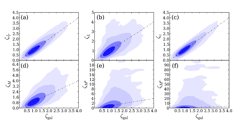
Figure 3.— Contour plots showing $\zeta_{\rm gal}$ vs. $\zeta_{q}$ for various weighting methods, as measured from numerical simulations. Dark to lighter shades refer to $1,2,3$, and $4\sigma$ regions, respectively. The dotted line marks $\zeta_{\rm gal}=\zeta_{q}$. We see that the different $\zeta_{q}$ are correlated, i.e. under/overdense LOSs in one metric are typically under/overdense in other metrics as well. However, they are not identical, implying that imposing multiple $\zeta_{q}$ conditions adds information and thus sharpens the PDF.

4.1.1 Weighting by Radius

The angular separation between the source and a nearby object is a significant factor in distorting, and thereby shaping, the path through which the source’s light passes. We expect then that each galaxy within $45^{\prime\prime}$ does not contribute equally, but that those nearer the optical axis of the lens are more influential than those farther away. In particular for isothermal total mass distributions (appropriate for massive galaxies or around the scale radius of halos, e.g., Gavazzi et al., 2007; Lagattuta et al., 2010), we expect the convergence to decline as the inverse projected distance from the deflector. This gives rise to our first weighting method of $1/r$. We will scale all objects that satisfy $10^{\prime\prime}<r\leq 45^{\prime\prime}$ by $1/r$. At $r\leq 10^{\prime\prime}$ weighting becomes sensitive to small changes in $r$. Thus for $r\leq 10^{\prime\prime}$ we allow each object to carry a weight of $1/10$, giving us a continuous weighting function. We note that in general objects that are very close to the main deflector are more likely to be physically associated with it and exert a stronger impact (e.g., Keeton & Zabludoff, 2004). Therefore it is prudent to model them explicitly, rather than considering them as part of the statistical lines of sight effect. This might require obtaining as much information as possible on them, including redshifts (Momcheva et al., 2006; Auger et al., 2007) and possibly stellar velocity dispersions, especially if they are consistent with massive galaxies.

4.1.2 Weighting by Redshift

Objects close to the source along the line of sight have minimal lensing effects from the scaled deflection of light rays. Likewise, those nearest to the observer are relatively insignificant. In order to approximately account for this, our next heuristic weighting method is quadratic in $z$ and defined as $z_{\rm source}\cdot z-z^{2}$ where $z_{\rm source}$ and $z$ are the redshifts of the source and the object along the LOS, respectively. For simplicity the notation of this weighting method is “$z$”.

4.1.3 Weighting by Stellar Mass

The most massive galaxies will produce detectable lensing effects over a larger area of the sky. Thus we choose one of the weighting methods to be $M^{n}$ where $M$ is the object’s stellar mass and $n$ is some positive integer. The rationale for this scaling is that at the high mass end of the galaxy stellar mass function, the relation between stellar mass and total mass is non-linear. According to, e.g., weak lensing, clustering, satellites, and abundance matching studies, the total mass increases with stellar mass faster than linear in for the most massive galaxies (Mandelbaum et al., 2006; Wake et al., 2011; Behroozi et al., 2010; Leauthaud et al., 2012; More et al., 2011). This is consistent with the fact that the central galaxies of massive clusters and poor groups do not typically differ in stellar mass by orders of magnitude even though their halos do. For $M^{n}$ with $n>1$ we will consider both $\sum_{i=1}^{N_{\rm gal}}M_{i}^{n}$ and $\sqrt[n]{\sum_{i=1}^{N_{\rm gal}}M_{i}^{n}}$. The former will be denoted as $W_{M^{n}}$ while the latter as the root sum of the squares $W_{M_{\rm rss}^{n}}$. In this paper we explore the cases of $n=1,2,$ and $3$. In this section we assume to know precisely the correct masses, as given by the Millennium catalog; in Section 5 we allow each mass to depend on its respective photometric redshift to assess the reliability of a $M^{n}$ weighting method.

4.1.4 Weighting by Luminosity

In practice, inferring the stellar mass of an object with limited observational data can be difficult, leading to large uncertainties. For this purpose we will also explore weighting by luminosity, $W_{L}$.

4.2. $\kappa_{\rm ext}$ PDF with New Statistics

We now proceed with the method outlined in Section 3, requiring that $\zeta_{q}=0.75,1.25,1.5$, or $2$ for all aforementioned $q$. Contour plots for $\zeta_{q}$ versus $\zeta_{\rm gal}$ given in Figure 3 show how the various relative overdensities are related. Because each weighting scheme differs in $\overline{W_{q}}$ from every other, we would like to ensure that keeping a consistent interval width $E$ does not affect our relative spread. Weighting schemes with low $\overline{W_{q}}$ would offer a higher percentage of total lines of sight than those with large $\overline{W_{q}}$. To normalize our spread we multiply each $W_{q}$ by $\frac{\overline{N_{\rm gal}}}{\overline{W_{q}}}$. Thus, we generalize Equation (1) to the following for new statistics:

$$\left\lvert\frac{\overline{N_{\rm gal}}}{\overline{W_{q}}}W_{q}-\zeta_{q}\overline{N_{\rm gal}}\right\rvert<E.$$ (3)

Furthermore, $W_{q}$ is no longer restricted to discrete integer values, but rather a continuum. Still, we expect $\frac{dN_{\rm LOS}}{dW_{q}}\neq 0$ at under- and overdense $\zeta_{q}$ so it is necessary to normalize by the inverse number of LOS. We allow $2E$ bins, each of length 1, from $\zeta_{q}\overline{N_{\rm gal}}-E$ to $\zeta_{q}\overline{N_{\rm gal}}+E$ (as previously done in Section 3 with discretely-valued $N_{\rm gal}$), and define $N_{\rm LOS}$ as the number of LOS within a particular bin. We then weight each $\kappa_{\rm ext}$ value by $\frac{1}{N_{\rm LOS}}$ of its respective bin when constructing the PDF.

The variables discussed in Section 4.1 are the principal contributors to gravitational lensing; however, using a single variable may be too basic of an approximation. We can expand our definition of Equation (2) to allow the weighted sum ($W_{q}$) to be the product of characteristics

$$W_{q}=\sum_{i=1}^{N_{\rm gal}}\prod_{j=1}^{n_{\rm var}}q_{ij}$$ (4)

where $n_{\rm var}$ is the number of variables. Figure 4 (the seven right-most set of bars) and Table 1 show that this leads to greater improvements in $\sigma_{\kappa}$ when combining $1/r$ with the established $q$, though in principle this can be done with any combination.

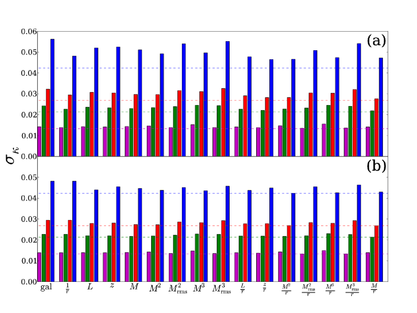
Figure 4.— Values for $\sigma_{\kappa}$ for various weighting schemes with (a) successive $\zeta_{\rm gal}$ and $\zeta_{q}$ conditions, and (b) successive $\zeta_{\rm gal}$, $\zeta_{q}$ and $\zeta_{\frac{1}{r}}$ conditions as measured from numerical simulations. As discussed in the text, note that cases where multiple conditions become equivalent (such as the leftmost bar in the top panel, corresponding to imposing two consecutive $\zeta_{\rm gal}$ conditions) amount to a redundancy and no new information is gained. The color scheme is the same as in previous plots: purple, green, red, and blue refer to $\zeta_{q}=0.75,1.25,1.5,$ and $2$, respectively. The horizontal dashed lines correspond to the lowest value of $\sigma_{\kappa}$ obtained through the weighting schemes considered. We find the uncertainty on $\kappa_{\rm ext}$ is reduced by imposing more conditions.

In addition to generalizing $W_{q}$, we can use Equation (3) to impose multiple $\zeta_{q}$ conditions. For example, we can require that LOS satisfy Equation (3) for both galaxy count and $1/r$ weighting. This is a more stringent demand, as LOS must now pass two separate cuts. Note that our respective $\zeta_{q}$ (in this example $\zeta_{\rm gal}$, $\zeta_{\frac{1}{r}}$) values need not be equivalent. However, for the sake of illustration in this paper we will assume they are. We refer to the number of applied conditions as $n_{\rm con}$. This imposes consecutive cuts that improve the quality of the $\kappa_{\rm ext}$ PDF, but reduce the number of LOS. As long as $n_{\rm con}$ is not chosen to be large enough to introduce statistical uncertainty, we expect a sharpening of the peak as remaining LOS will be more relevant to the lens of interest. We must, however, now expand our definition of $N_{\rm LOS}$ to incorporate combinations of every possible value between $\pm E$ for each of $n_{\rm con}$. Thus each LOS does not simply correspond to one of $2E$ values, but instead $\left(2E\right)^{n_{\rm con}}$.

We remind the reader that $\zeta_{q}$ refers to the relative overdensity of any of the aforementioned weights (e.g. galaxy counts, $1/r$, $z$, $L$, $M$). Using the prescribed method we measure $\sigma_{\kappa}$ for each weighting scheme. We do this by constructing the PDF from LOS that satisfy Equation (3) in three variations: (1) $\zeta_{q}$; (2) $\zeta_{q}$ and $\zeta_{\rm gal}$, and; (3) $\zeta_{q},\zeta_{\rm gal}$, and $\zeta_{\frac{1}{r}}$. It is worth noting that for case (2) this amounts to applying the same condition twice for $\zeta_{\rm gal}$, and in case (3) we have a similar redundancy for both $\zeta_{\rm gal}$ and $\zeta{\frac{1}{r}}$.

We expect that imposing more conditions, as in cases (2) and (3), would lead to a smaller width of the $\kappa_{\rm ext}$ PDF. Figure 4 shows $\sigma_{\kappa}$ for these latter two cases. There are several features here worth noting. First, changes in $\sigma_{\kappa}$ for $\zeta_{q}=0.75,1.25$, and $1.5$ are relatively small when compared with those for $\zeta_{q}=2$. Thus, it is most easy to detect any increase or decline in $\sigma_{\kappa}$ for $\zeta_{q}=2$. Second, if we assume that any change in $\sigma_{\kappa}$ for each $q$ at $\zeta_{q}=2$ is indicative of the change at lower $\zeta_{q}$ (albeit on a smaller scale), then we can restrict the analysis to $\zeta_{q}=2$ to determine which variables constrain $\kappa_{\rm ext}$ the most.

We also see that in all cases $\sigma_{\kappa}$ decreases when more conditions are imposed, as expected. Table 1 gives the values for the bars in Figure 4, along with $\zeta_{q}$ for case (1) as mentioned above. We note that for lenses with $\zeta_{q}\lesssim 1.5$ in multiple conditions, the uncertainty in $\kappa_{\rm ext}$ is reduced to $\lesssim 0.03$, a level that is comparable to or smaller than the strong lens mass modeling uncertainty in terms of its impact on the time-delay distance (e.g. Suyu et al., 2010, 2013). As current and future surveys are expected to discover at least hundreds of lenses (Oguri & Marshall, 2010), we expect an efficient sample for cosmographic studies to contain lenses with relative overdensities $\lesssim 1.5$. This will ensure that uncertainties due to the LOS structures are subdominant.

Table 1 Values of $\sigma_{\kappa}$ for $\zeta_{q}=2$ for various weighting methods and conditions.

$q$	$\zeta_{q}=2$	$\zeta_{\rm gal},\zeta_{q}=2$	$\zeta_{\rm gal},\zeta_{\frac{q}{r}}=2$	$\zeta_{\rm gal},\zeta_{q},\zeta_{\frac{1}{r}}=2$	$\zeta_{\rm gal},\zeta_{\frac{q}{r}},\zeta_{\frac{1}{r}}=2$
$\rm gal$	0.0562$\pm$0.0003	—	—	—	—
$\frac{1}{r}$	0.0534$\pm$0.0002	0.0481$\pm$0.0003	—	—	—
$L$	0.0464$\pm$0.0002	0.0520$\pm$0.0004	0.0478$\pm$0.0003	0.0440$\pm$0.0005	0.0437$\pm$0.0004
$z$	0.0507$\pm$0.0003	0.0525$\pm$0.0004	0.0464$\pm$0.0004	0.0455$\pm$0.0004	0.0449$\pm$0.0003
$M$	0.0382$\pm$0.0002	0.0511$\pm$0.0006	0.0472$\pm$0.0004	0.0447$\pm$0.0006	0.0430$\pm$0.0005
$M^{2}$	0.0319$\pm$0.0001	0.0492$\pm$0.0006	0.0466$\pm$0.0006	0.0438$\pm$0.0009	0.0423$\pm$0.0006
$M_{\rm rss}^{2}$	0.0449$\pm$0.0002	0.0540$\pm$0.0005	0.0508$\pm$0.0004	0.0451$\pm$0.0007	0.0454$\pm$0.0005
$M^{3}$	0.0319$\pm$0.0001	0.0496$\pm$0.0008	0.0474$\pm$0.0005	0.0436$\pm$0.0011	0.0425$\pm$0.0008
$M_{\rm rss}^{3}$	0.0417$\pm$0.0002	0.0551$\pm$0.0007	0.0541$\pm$0.0005	0.0458$\pm$0.0008	0.0464$\pm$0.0005

Notes. The $\sigma_{\kappa}$ measured from numerical simulations decrease with some of the unique condition $\zeta_{q}=2$ (second column) because they incorporate a large range of $\zeta_{\rm gal}$ values not necessarily correspondent to $\zeta_{\rm gal}=2$. This problem is fixed by always imposing initial condition $\zeta_{\rm gal}=2$ (columns 3–6).

The spread of $\kappa_{\rm ext}$ for $\zeta_{q}=2$ in Table 1 is easily explained by Figure 3. If we look at $\zeta_{q}=2$ for $\zeta_{q}\neq\zeta_{\rm gal}$ we see that a majority of its $\zeta_{\rm gal}$ values lie at $\zeta_{\rm gal}<2$. This causes a shift in the overall $\kappa_{\rm ext}$ distribution, lowering the median and shrinking $\sigma_{\kappa}$. Therefore, such a decrease is not the result of improving our method to find $\kappa_{\rm ext}$, but the inclusion of a large number of small $\kappa_{\rm ext}$ values with $\zeta_{\rm gal}<2$. This reiterates the effectiveness of imposing $\zeta_{\rm gal}$ and other $\zeta_{q}$ conditions, as in Figure 4 and the remaining columns of Table 1.

While all weighting methods lead to a decrease in $\sigma_{\kappa}$, the lowest values are for $W_{\frac{M^{n}}{r}}$. For the $\kappa_{\rm ext}$ PDFs that include the $\zeta_{\rm gal}$ constraint, the weighting scheme that leads to the tightest PDF is $\zeta_{\rm gal},\zeta_{\frac{M^{2}}{r}},\zeta_{\frac{1}{r}}=2$ with the corresponding PDF width as $\sigma_{\kappa}=0.0423\pm 0.0006$ (see columns 3 to 6 in Table 1). This is a substantial drop from our initial finding of $\sigma_{\kappa}=0.0562\pm 0.0003$ for $\zeta_{\rm gal}=2$, and $\sigma_{\kappa}\sim 0.065$ that was obtained by Suyu et al. (2010) for B1608 without applying the $z<1.4$ cut.

5. Testing the fidelity of $\kappa_{\rm ext}$ estimates based on photometric redshifts

Until this point our simulated galaxy catalogs from the Millennium Simulation have allowed us to neglect uncertainties in redshift and stellar mass that would normally arise from observations. However, getting spectroscopic redshifts for a large sample of objects – many at $z>1$ – is difficult and expensive. It is thus prudent to focus spectroscopic resources on the brighter objects and those closer to the main deflector, while using photometric redshifts for the remaining objects along the line of sight. Because a galaxy’s estimated stellar mass and luminosity are dependent on its redshift, their uncertainties are sensitive to errors in $z$. It is necessary then to estimate the uncertainties in $\kappa_{\rm ext}$ associated with obtaining redshifts photometrically.

5.1. Estimating photometric redshifts

The Millennium Simulation gives magnitudes for SDSS u, g, r, i, z and 2MASS J, H, K bands. We use the Bayesian Photometric Redshift (hereafter BPZ; Benítez, 2000; Coe et al., 2006) program to calculate the photometric redshift $z_{\rm phot}$, which is defined as the peak of the redshift PDF, for all objects. To evaluate how $\kappa_{\rm ext}$ is affected by the quality of $z_{\rm phot}$, we examine three different band combinations. First of all, we use ugrizJHK to compute what we may assume to be the best approximation to $z_{\rm spec}$. Secondly, we use g, r, i, and K bands, in an effort to strike a compromise between survey speed and wavelength coverage, as a measure of the effectiveness of our method when only a few bands are available. Lastly, we compute $z_{\rm phot}$ using just g, r, and i bands to evaluate how our method holds under the least number of bands from which a redshift might be computed. Typically, optical bands such as g, r, and i are the most readily available or do not require long integration times, which make them ideal for large-scale surveys.

5.2. Calculating $\kappa_{\rm ext}^{\rm med}$ based on galaxy number counts with photometric data

The errors associated with photometric redshifts are expected to decrease as wavelength coverage is increased. However, in practice obtaining ugrizJHK is observationally expensive. Thus this section serves primarily as a premise for the optimal strategies associated with photometrically determining $z$.

Table 2Values of the shifts $\Delta\kappa_{\rm ext}^{\rm med}$ and $\Delta\sigma_{\kappa}$ with $\zeta_{q}=2$ for $z_{\rm phot}$ computed using a variety of band combinations.

$q$	$\rm ugrizJHK$		$\rm griK$		$\rm gri$
	$\Delta\kappa_{\rm ext}^{\rm med}$	$\Delta\sigma_{\kappa}$	$\Delta\kappa_{\rm ext}^{\rm med}$	$\Delta\sigma_{\kappa}$	$\Delta\kappa_{\rm ext}^{\rm med}$	$\Delta\sigma_{\kappa}$
$\rm gal$	0.0060$\pm$0.0003	0.0023$\pm$0.0002	0.0066$\pm$0.0005	0.0026$\pm$0.0005	0.0155$\pm$0.0008	0.0063$\pm$0.0005
$\frac{1}{r}$	0.0075$\pm$0.0003	0.0034$\pm$0.0003	0.0079$\pm$0.0005	0.0025$\pm$0.0005	0.0151$\pm$0.0008	0.0051$\pm$0.0005
$L$	0.0071$\pm$0.0008	0.0041$\pm$0.0009	0.0075$\pm$0.0011	0.0038$\pm$0.0019	0.0145$\pm$0.0013	0.0060$\pm$0.0019
$z$	0.0063$\pm$0.0011	0.0039$\pm$0.0007	0.0127$\pm$0.0017	0.0086$\pm$0.0013	0.0219$\pm$0.0021	0.0116$\pm$0.0013
$M$	0.0054$\pm$0.0012	0.0022$\pm$0.0011	0.0025$\pm$0.0009	0.0020$\pm$0.0015	0.0168$\pm$0.0011	0.0065$\pm$0.0015
$M^{2}$	0.0067$\pm$0.0022	0.0029$\pm$0.0028	0.0050$\pm$0.0008	0.0028$\pm$0.0022	0.0142$\pm$0.0008	0.0042$\pm$0.0022
$M_{\rm rss}^{2}$	0.0103$\pm$0.0008	0.0047$\pm$0.0021	0.0105$\pm$0.0027	0.0052$\pm$0.0023	0.0202$\pm$0.0025	0.0076$\pm$0.0023
$M^{3}$	0.0047$\pm$0.0015	0.0041$\pm$0.0029	0.0159$\pm$0.0059	0.0085$\pm$0.0021	0.0148$\pm$0.0025	0.0068$\pm$0.0021
$M_{\rm rss}^{3}$	0.0080$\pm$0.0012	0.0064$\pm$0.0015	0.0124$\pm$0.0046	0.0033$\pm$0.0019	0.0190$\pm$0.0012	0.0085$\pm$0.0019
$\frac{L}{r}$	0.0077$\pm$0.0012	0.0041$\pm$0.0007	0.0077$\pm$0.0013	0.0029$\pm$0.0016	0.0115$\pm$0.0015	0.0032$\pm$0.0016
$\frac{z}{r}$	0.0025$\pm$0.0007	0.0017$\pm$0.0009	0.0047$\pm$0.0008	0.0026$\pm$0.0007	0.0143$\pm$0.0011	0.0045$\pm$0.0007
$\frac{M^{2}}{r}$	0.0061$\pm$0.0009	0.0028$\pm$0.0007	0.0077$\pm$0.0011	0.0021$\pm$0.0015	0.0122$\pm$0.0015	0.0043$\pm$0.0015
$\frac{M_{\rm rss}^{2}}{r}$	0.0116$\pm$0.0010	0.0049$\pm$0.0007	0.0121$\pm$0.0017	0.0049$\pm$0.0017	0.0203$\pm$0.0017	0.0072$\pm$0.0017
$\frac{M^{3}}{r}$	0.0085$\pm$0.0007	0.0047$\pm$0.0009	0.0264$\pm$0.0037	0.0131$\pm$0.0017	0.0128$\pm$0.0018	0.0036$\pm$0.0017
$\frac{M_{\rm rss}^{3}}{r}$	0.0109$\pm$0.0013	0.0053$\pm$0.0017	0.0100$\pm$0.0019	0.0071$\pm$0.0021	0.0136$\pm$0.0023	0.0051$\pm$0.0021
$\frac{M}{r}$	0.0056$\pm$0.0006	0.0015$\pm$0.0009	0.0017$\pm$0.0011	0.0006$\pm$0.0017	0.0194$\pm$0.0012	0.0051$\pm$0.0017

In Figure 5, we plot $\kappa_{\rm ext}$ PDFs for $N_{\rm gal}$ with the original requirement of Equation (1) for $\zeta_{\rm gal}=0.75,1.25,1.5$, and $2$ based on the spectroscopic redshifts (solid) and various photometric-redshift estimations (dashed, dot-dashed, dotted). With photometric-$z$ computed using all 8-bands, we recover the overall shape of the $\kappa_{\rm ext}$ PDF. The $\kappa_{\rm ext}$ PDF based on griK is shown only for $\zeta_{\rm gal}=2$, which is nearly indistinguishable from the one based on all bands. It is evident that fewer photometric bands causes a shift in $\kappa_{\rm ext}$ toward higher values. This is consistent with the fact that with only gri BPZ tends to produce photo-z with large uncertainties and slightly low bias. Thus, high redshift objects are incorrectly assigned $z<1.4$ and vice versa, but the net exchange favors an increase in objects with $z_{\rm phot}<1.4$. If we assume these underestimated high-$z$ objects are unlikely to be correlated with already overdense regions for $z_{\rm spec}<1.4$ (a reasonable assumption), then a uniform increment, $\delta N_{\rm gal}$, is accounted for along each LOS. Thus our LOS of previous relative overdensities go from $\zeta_{\rm gal}\overline{N_{\rm gal}}\rightarrow\zeta_{\rm gal}\overline{N_{\rm gal}}+\delta N_{\rm gal}$, while our new mean becomes $\overline{N_{\rm gal}^{\prime}}=\overline{N_{\rm gal}}+\delta N_{\rm gal}$. Multiplying $\zeta_{\rm gal}$ by $\overline{N_{\rm gal}^{\prime}}$, we find that our new count based on $z_{\rm phot}$ and satisfying (1) is $\zeta_{\rm gal}(\overline{N_{\rm gal}}+\delta N_{\rm gal})$, having $\delta N_{\rm gal}\left(\zeta_{\rm gal}-1\right)$ more galaxies than the previous selection criteria. Consequently, relative galaxy (over/under)densities based on photometric redshifts are associated with more (over/under)dense lines of sight compared to spectroscopy-based galaxy overdensities with the same nominal value. If one were to ignore the difference between photometric and spectroscopic redshifts, this would induce a bias in the estimation of $\kappa_{\rm ext}$. This bias is small when using ugrizJHK or even griK, but notable when only gri is available. It is possible, however, to further reduce such a bias by improving the photo-z to remove the small bias or by using exactly the same method of redshift determination in the actual observations and the simulations.

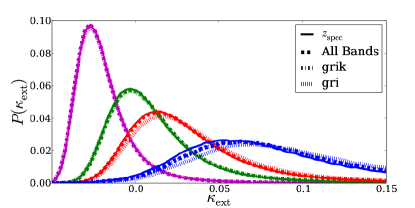
Figure 5.— $\kappa_{\rm ext}$ PDFs constructed from LOS satisfying Equation (1) for $\zeta_{\rm gal}=0.75$ (purple), $1.25$ (green), $1.5$ (red), and $2$ (blue) for spectroscopic (solid) and photometric redshifts as measured from numerical simulations. Photometric redshifts are computed using all available optical and infrared bands (dashed), griK bands (dot-dashed; shown for $\zeta_{\rm gal}=2$ only) and gri bands (dotted).

The accuracy of the $\kappa_{\rm ext}$ PDF should reflect the effectiveness of a band combination’s ability to estimate correctly an object’s redshift. To quantify this accuracy we define the change in PDF width $\Delta\sigma_{\kappa}\equiv\sigma_{\kappa}^{\rm phot}-\sigma_{\kappa}^{\rm true}$ where $\sigma_{\kappa}^{\rm phot}$ and $\sigma_{\kappa}^{\rm true}$ are the uncertainty in $\kappa_{\rm ext}$ for $z_{\rm phot}$ and $z_{\rm spec}$, respectively. Similarly, we define $\Delta\kappa_{\rm ext}^{\rm med}$ as the difference between the photometrically-determined $\kappa_{\rm ext}^{\rm med}$ and the spectroscopically-determined $\kappa_{\rm ext}^{\rm med}$. We expect these quantities to be the smallest for $z_{\rm phot}$ with all 8 bands, and to increase as fewer bands are used in constructing the redshift. The first row of Table 2 shows that with all 8 bands or with even only griK, the change in the $\kappa_{\rm ext}$ PDF is $<$0.007, corresponding to $<$0.7% impact on the time-delay distance. We thus conclude that the minimal set of filters necessary to achieve a 1% precision and accuracy on time-delay distance (see Suyu et al., 2012, for a summary of cosmological implications) is three optical filters plus K.

5.3. Impact of photometric redshifts on accuracy and precision of $\kappa_{\rm ext}$ estimates using multiple weights

Because Section 4 demonstrated that using characteristic features of galaxies provides a sharper PDF we need to explore how photometric redshifts affect these weights and their respective PDFs. Specifically, we would like to confirm our intuition that these weighted PDFs behave in the same manner as their spectroscopic counterparts, so that we may choose a universal optimal weighting method that is independent of how an object’s attributes are obtained.

We use our photometric redshifts for $W_{z}$ and rescale the Millennium Simulation masses and luminosities by $\left(\frac{d_{\rm L}\left(z_{\rm phot}\right)}{d_{\rm L}\left(z_{\rm spec}\right)}\right)^{2}$ where $d_{\rm L}\left(z\right)$ is the luminosity distance at redshift $z$. This is a reasonable approximation for stellar mass, as to first order it scales proportional to luminosity. Table 2 lists the changes in the median $\Delta\kappa_{\rm ext}^{\rm med}=\kappa_{\rm ext}^{\rm med,phot}-\kappa_{\rm ext}^{\rm med,spec}$ and spread $\Delta\sigma_{\kappa}=\sigma_{\kappa}^{\rm phot}-\sigma_{\kappa}^{\rm spec}$ of the convergence distributions. We find that for nearly all $q$, $\Delta\sigma_{\kappa}$ increases with fewer bands, which is consistent with our observations for $\zeta_{\rm gal}$. However, when using either all bands or griK, the changes are below $0.01$ for a majority of the $q$.

We thus conclude that, as in the previous section, one should use as much information as possible to infer $P(\kappa_{\rm ext})$ for the observed line of sight. As shown in Figure 3, observables like position, luminosity, redshift, and stellar mass add valuable information and can improve both the precision (by reducing $\sigma_{\kappa}$) and the accuracy (by shifting $\kappa_{\rm ext}^{\rm med}$ closer to the “true” value) of the inference. In case spectroscopic redshifts are not available, we recommend using at least three optical bands and one infrared band for the weighting schemes considered in this paper. For the current level of cosmological precision and accuracy, using griK is sufficient to constrain $\kappa_{\rm ext}$ almost as well as with spectroscopic redshifts.

6. ILLUSTRATING THE METHOD WITH THE CASE STUDY B1608+656

The previous sections outlined a new approach for determining $\kappa_{\rm ext}$ for an arbitrary lens given that sufficient characteristics are known to calculate the relevant $\zeta_{q}$. In this section we illustrate how the method works in practice using B1608$+$656 as a case study. The data on the B1608$+$656 field includes deep HST imaging in F555W and F814W (9 and 11 orbits, respectively; GO-10158, PI Fassnacht), as well as more shallow imaging in Gunn g, r, and i obtained with the Palomar 60-Inch Telescope (full details of the observations can be found in Fassnacht et al., 2006). This section should be taken as an illustration only, since the data in hand for B1608$+$656 are not sufficient to achieve the full potential of our method. Therefore we do not revisit the cosmological implications of B1608$+$656 in this work. Work is in progress to collect the necessary photometry and spectroscopy and future papers will present improved estimates of $\kappa_{\rm ext}$ and cosmological parameters for B1608$+$656 and other systems.

6.1. Field Preparation and $W_{q}$

As a reference, we use the central portion ($1.1\times 1.1$ deg²) of the COSMOS field (Cosmic Evolution Survey; Scoville et al., 2007) as a sample for measuring the average number of galaxies and also the average properties of the features for all lines of sight, i.e., $\overline{W_{q}}$. COSMOS data, like B1608$+$656 data, has ACS F814W photometry that is sufficiently deep to satisfy the upper limit of the $I$ magnitude cut. We use the 2006 ACS Catalog (Leauthaud et al., 2007) and match the galaxies to those in the 2006 Photometry Catalog (Capak et al., 2007) in order to obtain redshifts and stellar masses. We consider two objects in opposing catalogs to be identical if they have angular separation $\leq 0.5^{\prime\prime}$. Of the $\sim 124,000$ objects in the ACS databank with $18.5<m_{\rm F814}<24.5$, approximately $118,000$ or $95\%$ have photometric coordinate-matched counterparts. Only $\sim 60$ ACS objects are found to be $\leq 0.5^{\prime\prime}$ to two different objects from the photometry catalog. In these few cases of ambiguous identification, the stellar mass from the multiband photometric catalog (Ilbert et al., 2010) is assigned to objects in the ACS catalog proportional to their fractional contribution to the total flux.

Because a small subsample of the ACS catalog does not have matches in the photometric database, we expect our mean relative overdensity values for all but $\zeta_{\rm gal}$ and $\zeta_{1/r}$ to be slightly underestimated. As a solution, a correction factor $b=N_{\rm ACS}/N_{\rm phot}$ is applied where $N_{\rm ACS}$ and $N_{\rm phot}$ are the total and matched number of galaxies in the ACS catalog, respectively. Thus multiplying the average number of galaxies that are found in the Photometry Catalog by $b$ results in the true average. This is not so apparent with other weighting methods, as simply multiplying $\overline{W_{q}}$ by the inverse fraction of galaxies detected with ground-based photometry assumes the missing subset is representative of the entire ACS catalog. Nonetheless, given that the $N_{\rm ACS}$ and $N_{\rm phot}$ only differ at the $5\%$ level, we expect the effects of such an assumption to be small.

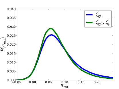
Figure 6.— $\kappa_{\rm ext}$ PDFs for $\zeta_{\rm gal}$ and $\zeta_{\frac{1}{r}}$ values as measured from B1608$+$656.

Table 3 Statistics of B1608$+$656 relative to COSMOS

$q$	$\overline{W_{q}}$	$W_{q}$	$\zeta_{q}$	$\kappa_{\rm ext}^{\rm med}$	$\sigma_{\kappa}$	$N_{\rm LOS}$
	(COSMOS)	(B1608$+$656)
$\rm gal$	41.6	83	1.997	0.0808	0.0562	2123167
$\frac{1}{r}$	3.1799	6.2928	1.979	0.0741	0.0471	527734
$z$	15.6181	30.6207	1.961	0.0784	0.0534	328798
$\frac{z}{r}$	1.1947	2.3658	1.980	0.0695	0.0464	314931

Notes. Column 1 lists the statistic, Column 2 are the average weights from lines of sight in COSMOS, Column 3 are the weights for B1608$+$656, and Column 4 are the relative overdensities (the ratio of Column 3 to Column 2). Columns 5 and 6 are, respectively, $\kappa_{\rm ext}$ and $\sigma_{\kappa}$ values found with all Millennium Simulation LOS that satisfy Equation (3) for both $\zeta_{\rm gal}$ and $\zeta_{q}$ conditions imposed. The number of LOS found from the Millennium data is also provided in Column 7 to indicate the reliability of the data.

To determine $W_{q}$ for B1608$+$656, we identify objects in the field of B1608$+$656 using SExtractor (Bertin & Arnouts, 1996). To ensure a fair comparison with COSMOS, we use only a single HST orbit of imaging (so that the COSMOS and B1608$+$656 images have similar depths), and follow the reduction steps outlined in Leauthaud et al. (2007), with the exception of masking out asteroid trails, oversaturated stars, etc. since these are not present within $45^{\prime\prime}$ of B1608$+$656. Once a catalog of all objects with $r<45^{\prime\prime}$ and $18.5<m_{\rm F814}<24.5$ has been created, the objects are coordinate-matched with a deeper catalog, constructed from the full 11 HST orbits of imaging. This second catalog serves two purposes: (1) to exclude fake detections from the single orbit SExtractor data set, and (2) to produce more reliable redshifts and stellar masses necessary to find $\zeta_{q}$ for the detected objects in the single-orbit catalog. A limited number of objects ($\sim 15$) have spectroscopic redshifts, or Gunn g, r, and i bands from ground-based imaging. Most, however, have just F814W and F606W photometries that make it difficult to obtain accurate stellar masses and photometric redshifts.

6.2. Finding $\zeta_{q}$ for B1608

We impose $z<1.4$ for COSMOS and B1608$+$656. We find that the observed average number of galaxies in COSMOS is $\overline{N_{\rm gal}}=41.6$ while B1608$+$656 has $83$ galaxies within $45^{\prime\prime}$, giving $\zeta_{\rm gal}=1.99$. This is close to $\zeta_{\rm gal}=2.18$ as found by Fassnacht et al. (2011) by comparing the galaxy counts to those in pure-parallel fields. The slight difference in $\zeta_{\rm gal}$ could be due to (1) our imposed redshift restriction $z<z_{\rm source}$ that was not applied by Fassnacht et al. (2011), and (2) the COSMOS field being slightly overdense. However, it is not clear how much COSMOS is overdense when the redshift condition is imposed. For simplicity, we neglect this correction, though in the future this will need to be measured before applying it to time-delay systems for cosmological inferences. In a method analogous to Section 4 we compute $\zeta_{q}$ for each characteristic, the results of which can be seen in Table 3 for characteristics that are computed with a higher degree of accuracy (e.g., $1/r$). Unfortunately the present data are not sufficient to estimate reliable stellar masses, luminosities, or accurate photometric redshifts. Deeper optical and NIR imaging of the field are necessary to obtain more accurate redshifts (see Table 2), luminosities, and stellar masses for computing $\zeta_{q}$.

Next we select from the Millennium Simulation lines of sight with the new $\zeta_{q}$ values to find $\kappa_{\rm ext}$. In keeping with Section 4 we impose Equation (3) for both $\zeta_{\rm gal}$ and $\zeta_{q}$ and find $\kappa_{\rm ext}$ and $\sigma_{\kappa}$ for the resulting distribution. These, along with the number of lines of sight, are given in the last three columns of Table 3. Distributions with $\zeta_{\rm gal}\sim\zeta_{q}$ are closely correlated and therefore have large $N_{\rm LOS}$. In Figure 6, we show the $\kappa_{\rm ext}$ PDF for B1608$+$656 with (1) only $\zeta_{\rm gal}$ imposed, and (2) both $\zeta_{\rm gal}$ and $\zeta_{1/r}$ conditions imposed. The additional $\zeta_{1/r}$ condition sharpens the PDF, leading to a decrease in $\sigma_{\kappa}$ from 0.056 by $\sim 0.01$. In this specific case of B1608$+$656, the new $\kappa_{\rm ext}$ PDF does not decrease the uncertainty on the final time-delay distance measurement appreciably since the stellar kinematics of the lens galaxy provides substantial constraints on $\kappa_{\rm ext}$ already, similar to the level that is achieved with the multiple $\zeta_{q}$ conditions. Nonetheless, the PDF of the time-delay distance is shifted to lower values by $1-2\%$ due to the lower $\kappa_{\rm ext}^{\rm med}$. We thus conclude that even though these effects are smaller than current uncertainties for a single lens, they will become important for reaching the ultimate goal of 1% precision and accuracy.

To generalize, without the velocity dispersion as a constraint, the new $\kappa_{\rm ext}$ would have decreased the uncertainty on the resulting $H_{0}$ from B1608$+$656 for various uniform cosmological priors by $\sim 1\,\rm{km\,s^{-1}\,Mpc^{-1}}$ from $\sim 4\,\rm{km\,s^{-1}\,Mpc^{-1}}$. Therefore, for lens systems in which the lens velocity dispersion is difficult to obtain (due to, e.g., bright lensed images that are near the lens galaxies), or for very large samples for which stellar velocity dispersions might not be practical, our techniques for tightening $\kappa_{\rm ext}$ are especially valuable since the reduction in the uncertainty on $\kappa_{\rm ext}$ would then translate directly to that on the time-delay distance (e.g., $0.01$ in $\kappa_{\rm ext}$ is approximately 1% on the time-delay distance).

7. SUMMARY AND CONCLUSIONS

With the goal of finding ways to measure the effects of the distribution of mass along the line of sight to gravitational lensing time delays, we have performed a comprehensive analysis of simulated lines of sight catalogs. These lines of sight catalogs are based on the Millennium Simulation, used to compute the external convergence $\kappa_{\rm ext}$ via ray-tracing, as well as on semianalytic models of galaxy formation, used to assign observable properties to halos along the line of sight.

Our main results can be summarized as follows

1. The observed relative abundance of galaxies within a given aperture $\zeta_{\rm gal}$ provides an estimate of $\kappa_{\rm ext}$ that is accurate to a few percent, depending on the actual under/overdensity of the observed line of sight. This is consistent with previous work (Suyu et al., 2010).

2. Adding information from other observables like stellar mass, luminosity, redshift, position of the galaxies in the vicinity of the main deflector, reduces significantly the uncertainty in $\kappa_{\rm ext}$. The most significant drop in uncertainty is obtained by weighting each galaxy with the inverse of the projected distance to the main deflector, followed by powers of the stellar mass. With this kind of information the uncertainty on time-delay distance arising from $\kappa_{\rm ext}$ can be reduced to $\sim 4$% from $\sim 6$% using only galaxy counts for a very overdense line of sight and to $\sim 3$% for typical lines of sight.

3. Even though spectroscopic redshifts are valuable, especially for the galaxies most closely associated with the main deflector, photometry in three optical bands (e.g., gri) and the near infrared (K) are sufficient for obtaining photometric redshifts such that the median and width of the $\kappa_{\rm ext}$ change by $<0.007$, i.e., $<0.7\%$ on the time-delay distance.

4. As a practical illustration, we apply this method to the field of B1608$+$656 and show that some gain can be made even with existing data. Better multiband photometry is needed to fully realize the gains promised by our method.

From these results, we conclude that with sufficient imaging and spectroscopy data the effects of the mass distribution along the line of sight on gravitational time-delay distances can be accounted for and the associated uncertainties reduced for all lines of sight. These improvements – in combination with recent advances in the derivation of gravitational time delays (Tewes et al., 2012) and in the modeling of the mass distribution of the main deflector and objects in close proximity to it (Suyu et al., 2013) – bring us closer to the goal of 1% precision in cosmological distances, necessary to address fundamental issues such as the nature of dark energy (Suyu et al., 2012).

In the next decade, upcoming surveys are expected to deliver thousands of gravitationally lensed quasars (Oguri & Marshall, 2010), a number more than sufficient to meet the 1% goal provided effort is made to keep systematic uncertainties under control. This will have to include theoretical uncertainties related to the choice of numerical simulations and associated semianalytic models. Our choice of using overdensities with respect to random fields, as opposed to absolute densities, minimizes the impact of the choice of this specific model. However, as the number of lenses with measured time delays increases thus reducing the observational errors toward the 1% level, it will be important to repeat and extend this study with independent cosmological simulations and galaxy formation models. This is left for future work.

From an observational point of view, the future abundance of targets will change dramatically the situation with respect to the present time when the precision of time-delay cosmology is limited by the number of known strongly lensed quasars, and allow us to choose the targets that give more cosmological information at fixed observational resources. This work suggests that focusing follow-up efforts on specific lines of sight – those that are not too overdense with respect to the average of the universe – should result in substantial gains in efficiency.

References

- Auger et al. (2007) Auger, M. W., Fassnacht, C. D., Abrahamse, A. L., Lubin, L. M., & Squires, G. K. 2007, AJ, 134, 668
- Auger et al. (2010) Auger, M. W., Treu, T., Bolton, A. S., et al. 2010, ApJ, 724, 511
- Bar-Kana (1996) Bar-Kana, R. 1996, ApJ, 468, 17
- Barnabè et al. (2009) Barnabè, M., Czoske, O., Koopmans, L. V. E., et al. 2009, MNRAS, 399, 21
- Bartelmann (2010) Bartelmann, M. 2010, Classical and Quantum Gravity, 27, 233001
- Behroozi et al. (2010) Behroozi, P. S., Conroy, C., & Wechsler, R. H. 2010, ApJ, 717, 379
- Benítez (2000) Benítez, N. 2000, ApJ, 536, 571
- Bertin & Arnouts (1996) Bertin, E. & Arnouts, S. 1996, A&AS, 117, 393
- Bradač et al. (2004) Bradač, M., Lombardi, M., & Schneider, P. 2004, A&A, 424, 13
- Broadhurst et al. (1995) Broadhurst, T. J., Taylor, A. N., & Peacock, J. A. 1995, ApJ, 438, 49
- Capak et al. (2007) Capak, P., Aussel, H., Ajiki, M., McCracken, H. J., Mobasher, B., Scoville, N., Shopbell, P., Taniguchi, Y., Thompson, D., Tribiano, S., Sasaki, S., Blain, A. W., Brusa, M., Carilli, C., Comastri, A., Carollo, C. M., Cassata, P., Colbert, J., Ellis, R. S., Elvis, M., Giavalisco, M., Green, W., Guzzo, L., Hasinger, G., Ilbert, O., Impey, C., Jahnke, K., Kartaltepe, J., Kneib, J.-P., Koda, J., Koekemoer, A., Komiyama, Y., Leauthaud, A., Le Fevre, O., Lilly, S., Liu, C., Massey, R., Miyazaki, S., Murayama, T., Nagao, T., Peacock, J. A., Pickles, A., Porciani, C., Renzini, A., Rhodes, J., Rich, M., Salvato, M., Sanders, D. B., Scarlata, C., Schiminovich, D., Schinnerer, E., Scodeggio, M., Sheth, K., Shioya, Y., Tasca, L. A. M., Taylor, J. E., Yan, L., & Zamorani, G. 2007, ApJS, 172, 99
- Coe et al. (2006) Coe, D., Benítez, N., Sánchez, S. F., Jee, M., Bouwens, R., & Ford, H. 2006, AJ, 132, 926
- Coe & Moustakas (2009) Coe, D. & Moustakas, L. A. 2009, ApJ, 706, 45
- Courbin et al. (2011) Courbin, F., Chantry, V., Revaz, Y., Sluse, D., Faure, C., Tewes, M., Eulaers, E., Koleva, M., Asfandiyarov, I., Dye, S., Magain, P., van Winckel, H., Coles, J., Saha, P., Ibrahimov, M., & Meylan, G. 2011, A&A, 536, A53
- Courbin et al. (2002) Courbin, F., Saha, P., & Schechter, P. L. 2002, in Lecture Notes in Physics, Berlin Springer Verlag, Vol. 608, Gravitational Lensing: An Astrophysical Tool, ed. F. Courbin & D. Minniti, 1
- Das & Linder (2012) Das, S. & Linder, E. V. 2012, ArXiv e-prints (1207.1105)
- Dobke et al. (2009) Dobke, B. M., King, L. J., Fassnacht, C. D., & Auger, M. W. 2009, MNRAS, 397, 311
- Ellis et al. (2001) Ellis, R., Santos, M. R., Kneib, J.-P., & Kuijken, K. 2001, ApJ, 560, L119
- Falco et al. (1985) Falco, E. E., Gorenstein, M. V., & Shapiro, I. I. 1985, ApJ, 289, L1
- Fassnacht et al. (2006) Fassnacht, C. D., Gal, R. R., Lubin, L. M., McKean, J. P., Squires, G. K., & Readhead, A. C. S. 2006, ApJ, 642, 30
- Fassnacht et al. (2011) Fassnacht, C. D., Koopmans, L. V. E., & Wong, K. C. 2011, MNRAS, 410, 2167
- Fassnacht et al. (1996) Fassnacht, C. D., Womble, D. S., Neugebauer, G., Browne, I. W. A., Readhead, A. C. S., Matthews, K., & Pearson, T. J. 1996, ApJ, 460, L103+
- Fassnacht et al. (2002) Fassnacht, C. D., Xanthopoulos, E., Koopmans, L. V. E., & Rusin, D. 2002, ApJ, 581, 823
- Fohlmeister et al. (2008) Fohlmeister, J., Kochanek, C. S., Falco, E. E., Morgan, C. W., & Wambsganss, J. 2008, ApJ, 676, 761
- Gavazzi et al. (2007) Gavazzi, R., Treu, T., Rhodes, J. D., Koopmans, L. V. E., Bolton, A. S., Burles, S., Massey, R. J., & Moustakas, L. A. 2007, ApJ, 667, 176
- Guo et al. (2011) Guo, Q., White, S., Boylan-Kolchin, M., De Lucia, G., Kauffmann, G., Lemson, G., Li, C., Springel, V., & Weinmann, S. 2011, MNRAS, 413, 101
- Hilbert et al. (2009) Hilbert, S., Hartlap, J., White, S. D. M., & Schneider, P. 2009, A&A, 499, 31
- Hilbert et al. (2007) Hilbert, S., White, S. D. M., Hartlap, J., & Schneider, P. 2007, MNRAS, 382, 121
- Hilbert et al. (2008) —. 2008, MNRAS, 386, 1845
- Hoekstra et al. (2011) Hoekstra, H., Hartlap, J., Hilbert, S., & van Uitert, E. 2011, MNRAS, 412, 2095
- Ilbert et al. (2010) Ilbert, O., Salvato, M., Le Floc’h, E., Aussel, H., Capak, P., McCracken, H. J., Mobasher, B., Kartaltepe, J., Scoville, N., Sanders, D. B., Arnouts, S., Bundy, K., Cassata, P., Kneib, J.-P., Koekemoer, A., Le Fèvre, O., Lilly, S., Surace, J., Taniguchi, Y., Tasca, L., Thompson, D., Tresse, L., Zamojski, M., Zamorani, G., & Zucca, E. 2010, ApJ, 709, 644
- Keeton (2010) Keeton, C. R. 2010, General Relativity and Gravitation, 42, 2151
- Keeton et al. (1997) Keeton, C. R., Kochanek, C. S., & Seljak, U. 1997, ApJ, 482, 604
- Keeton & Zabludoff (2004) Keeton, C. R. & Zabludoff, A. I. 2004, ApJ, 612, 660
- Kneib et al. (1993) Kneib, J. P., Mellier, Y., Fort, B., & Mathez, G. 1993, A&A, 273, 367
- Kneib et al. (2003) Kneib, J.-P. et al. 2003, ApJ, 598, 804
- Kneib & Natarajan (2011) Kneib, J.-P. & Natarajan, P. 2011, A&A Rev., 19, 47
- Kochanek (1991) Kochanek, C. S. 1991, ApJ, 373, 354
- Kochanek (1996) —. 1996, ApJ, 466, 638
- Koopmans et al. (2006) Koopmans, L. V. E., Treu, T., Bolton, A. S., Burles, S., & Moustakas, L. A. 2006, ApJ, 649, 599
- Koopmans & Treu (2003) Koopmans, L. V. E., & Treu, T. 2003, ApJ, 583, 606
- Lagattuta et al. (2010) Lagattuta, D. J., Fassnacht, C. D., Auger, M. W., Marshall, P. J., Bradač, M., Treu, T., Gavazzi, R., Schrabback, T., Faure, C., & Anguita, T. 2010, ApJ, 716, 1579
- Leauthaud et al. (2007) Leauthaud, A., Massey, R., Kneib, J.-P., Rhodes, J., Johnston, D. E., Capak, P., Heymans, C., Ellis, R. S., Koekemoer, A. M., Le Fèvre, O., Mellier, Y., Réfrégier, A., Robin, A. C., Scoville, N., Tasca, L., Taylor, J. E., & Van Waerbeke, L. 2007, ApJS, 172, 219
- Leauthaud et al. (2012) Leauthaud, A., Tinker, J., Bundy, K., Behroozi, P. S., Massey, R., Rhodes, J., George, M. R., Kneib, J.-P., Benson, A., Wechsler, R. H., Busha, M. T., Capak, P., Cortês, M., Ilbert, O., Koekemoer, A. M., Le Fèvre, O., Lilly, S., McCracken, H. J., Salvato, M., Schrabback, T., Scoville, N., Smith, T., & Taylor, J. E. 2012, ApJ, 744, 159
- Lemson & Virgo Consortium (2006) Lemson, G. & Virgo Consortium, t. 2006, ArXiv Astrophysics e-prints
- Limousin et al. (2007) Limousin, M., Richard, J., Jullo, E., Kneib, J.-P., Fort, B., Soucail, G., Elíasdóttir, Á., Natarajan, P., Ellis, R. S., Smail, I., Czoske, O., Smith, G. P., Hudelot, P., Bardeau, S., Ebeling, H., Egami, E., & Knudsen, K. K. 2007, ApJ, 668, 643
- Linder (2011) Linder, E. V. 2011, Phys. Rev. D, 84, 123529
- Mandelbaum et al. (2006) Mandelbaum, R., Seljak, U., Kauffmann, G., Hirata, C. M., & Brinkmann, J. 2006, MNRAS, 368, 715
- Meylan et al. (2006) Meylan, G., Jetzer, P., North, P., Schneider, P., Kochanek, C. S., & Wambsganss, J., eds. 2006, Gravitational Lensing: Strong, Weak and Micro
- Momcheva et al. (2006) Momcheva, I., Williams, K., Keeton, C., & Zabludoff, A. 2006, ApJ, 641, 169
- More et al. (2011) More, S., van den Bosch, F. C., Cacciato, M., Skibba, R., Mo, H. J., & Yang, X. 2011, MNRAS, 410, 210
- Oguri (2007) Oguri, M. 2007, ApJ, 660, 1
- Oguri & Marshall (2010) Oguri, M. & Marshall, P. J. 2010, MNRAS, 405, 2579
- Paraficz et al. (2009) Paraficz, D., Hjorth, J., & Elíasdóttir, Á. 2009, A&A, 499, 395
- Pettini et al. (2000) Pettini, M., Steidel, C. C., Adelberger, K. L., Dickinson, M., & Giavalisco, M. 2000, ApJ, 528, 96
- Richard et al. (2008) Richard, J., Stark, D. P., Ellis, R. S., George, M. R., Egami, E., Kneib, J.-P., & Smith, G. P. 2008, ApJ, 685, 705
- Refsdal (1964) Refsdal, S. 1964, MNRAS, 128, 307
- Saha (2000) Saha, P. 2000, AJ, 120, 1654
- Sand et al. (2008) Sand, D. J., Treu, T., Ellis, R. S., Smith, G. P., & Kneib, J.-P. 2008, ApJ, 674, 711
- Schechter et al. (1997) Schechter, P. L., Bailyn, C. D., Barr, R., et al. 1997, ApJ, 475, L85
- Schneider (1997) Schneider, P. 1997, MNRAS, 292, 673
- Schneider & Seitz (1995) Schneider, P. & Seitz, C. 1995, A&A, 294, 411
- Scoville et al. (2007) Scoville, N., Aussel, H., Brusa, M., Capak, P., Carollo, C. M., Elvis, M., Giavalisco, M., Guzzo, L., Hasinger, G., Impey, C., Kneib, J.-P., LeFevre, O., Lilly, S. J., Mobasher, B., Renzini, A., Rich, R. M., Sanders, D. B., Schinnerer, E., Schminovich, D., Shopbell, P., Taniguchi, Y., & Tyson, N. D. 2007, ApJS, 172, 1
- Seljak (1994) Seljak, U. 1994, ApJ, 436, 509
- Springel et al. (2005) Springel, V., White, S. D. M., Jenkins, A., Frenk, C. S., Yoshida, N., Gao, L., Navarro, J., Thacker, R., Croton, D., Helly, J., Peacock, J. A., Cole, S., Thomas, P., Couchman, H., Evrard, A., Colberg, J., & Pearce, F. 2005, Nature, 435, 629
- Sonnenfeld et al. (2011) Sonnenfeld, A., Bertin, G., & Lombardi, M. 2011, A&A, 532, A37
- Sonnenfeld et al. (2012) Sonnenfeld, A., Treu, T., Gavazzi, R., et al. 2012, ApJ, 752, 163
- Suyu et al. (2013) Suyu, S. H., Auger, M. W., Hilbert, S., Marshall, P. J., Tewes, M., Treu, T., Fassnacht, C. D., Koopmans, L. V. E., Sluse, D., Blandford, R. D., Courbin, F., & Meylan, G. 2013, ApJ, 766, 70
- Suyu et al. (2010) Suyu, S. H., Marshall, P. J., Auger, M. W., Hilbert, S., Blandford, R. D., Koopmans, L. V. E., Fassnacht, C. D., & Treu, T. 2010, ApJ, 711, 201
- Suyu et al. (2012) Suyu, S. H., Treu, T., Blandford, R. D., Freedman, W. L., Hilbert, S., Blake, C., Braatz, J., Courbin, F., Dunkley, J., Greenhill, L., Humphreys, E., Jha, S., Kirshner, R., Lo, K. Y., Macri, L., Madore, B. F., Marshall, P. J., Meylan, G., Mould, J., Reid, B., Reid, M., Riess, A., Schlegel, D., Scowcroft, V., & Verde, L. 2012, ArXiv e-prints (1202.4459)
- Tewes et al. (2012) Tewes, M., Courbin, F., Meylan, G., Kochanek, C. S., Eulaers, E., Cantale, N., Mosquera, A. M., Magain, P., Van Winckel, H., Sluse, D., Cataldi, G., Voros, D., & Dye, S. 2012, ArXiv e-prints (1208.6009)
- Treu (2010) Treu, T. 2010, ARA&A, 48, 87
- Treu et al. (2009) Treu, T., Gavazzi, R., Gorecki, A., Marshall, P. J., Koopmans, L. V. E., Bolton, A. S., Moustakas, L. A., & Burles, S. 2009, ApJ, 690, 670
- Treu & Koopmans (2002) Treu, T., & Koopmans, L. V. E. 2002, MNRAS, 337, L6
- Treu & Koopmans (2002) Treu, T. & Koopmans, L. V. E. 2002, ApJ, 575, 87
- Wake et al. (2011) Wake, D. A., Whitaker, K. E., Labbé, I., van Dokkum, P. G., Franx, M., Quadri, R., Brammer, G., Kriek, M., Lundgren, B. F., Marchesini, D., & Muzzin, A. 2011, ApJ, 728, 46
- Williams et al. (2008) Williams, K. A., Momcheva, I., Keeton, C. R., Zabludoff, A. I., & Lehár, J. 2008, ApJ, 672, 733
- Wong et al. (2011) Wong, K. C., Keeton, C. R., Williams, K. A., Momcheva, I. G., & Zabludoff, A. I. 2011, ApJ, 726, 84
- Wucknitz (2002) Wucknitz, O. 2002, MNRAS, 332, 951