CERN-PH-TH/2013-052
The universal Higgs fit
Pier Paolo Giardinoa,b, Kristjan Kannikec,d,
Isabella Masinae,f,
Martti Raidald,g
and Alessandro Strumiaa,d
(a) Dipartimento di Fisica, Università di Pisa and INFN, Italy
(b) CERN, Theory Division, CH-1211 Geneva 23, Switzerland
(c) Scuola Normale Superiore and INFN, Piazza dei Cavalieri 7, 56126 Pisa, Italy
(d) National Institute of Chemical Physics and Biophysics, Rävala 10, Tallinn, Estonia
(e) Dipartimento di Fisica e Scienze della Terra dell’Università di Ferrara and INFN, Italy
(f) CP3-Origins and DIAS, Southern Denmark University, Denmark
(g) Institute of Physics, University of Tartu, Estonia
Abstract
We perform a state-of-the-art global fit to all Higgs data. We synthesise them into a ‘universal’ form, which allows to easily test any desired model. We apply the proposed methodology to extract from data the Higgs branching ratios, production cross sections, couplings and to analyse composite Higgs models, models with extra Higgs doublets, supersymmetry, extra particles in the loops, anomalous top couplings, and invisible Higgs decays into Dark Matter. Best fit regions lie around the Standard Model predictions and are well approximated by our ‘universal’ fit. Latest data exclude the dilaton as an alternative to the Higgs, and disfavour fits with negative Yukawa couplings. We derive for the first time the SM Higgs boson mass from the measured rates, rather than from the peak positions, obtaining .
1 Introduction
After the discovery of a new particle around 125.5 GeV announced by the ATLAS [1] and CMS [2] LHC collaborations during 2012, all LHC and Tevatron collaborations presented at the Moriond 2013 conference their new results based on the full collected data. These include the most important and channels as well as updates to the fermionic channels. Such results will stay with us for next two years until LHC with full energy starts operating. Therefore it is the right moment to analyse their implications.
We want to know if the new particle is the long-waited Standard Model (SM) Higgs boson [3, 4, 5, 6]. On one side, the experimental collaborations are measuring its discrete quantum numbers to check if it is a scalar. On the other side, various theoretical groups [7] started to approximatively reconstruct from data its production cross section and its decay modes and consequently its couplings to check if they agree with the SM predictions or with other models beyond the SM. Clearly, this is a more significant test that can be precisely done only by the experimental collaborations, which indeed started to present analyses along these lines. However these experimental fits, presented in the form of likelihood plots within a few specific beyond-the-SM models, are of little use to theorists who are interested in different models.
We here propose how experimental collaborations could report their results in a model-independent and useful way, such that these results would be readily and reliably used by theorists who want to test any desired model. The new ingredient that we introduce and that allows for this simplification is the assumption that new physics can be approximated as a first-order perturbation with respect to the SM predictions. We find that this assumption is increasingly supported by measurements, that agree with the SM with precisions around the 20% level.
Such results, obtained after two years of LHC operation and with only 25/fb data per experiment, implies severe constraints on models where the Higgs boson is a portal to new physics. We analyse several models and rule out alternative scenarios to the Higgs boson.
The paper is organised as follows. In section 2 we present the data and our fitting procedure. In section 3 we derive the first measurement of the Higgs mass from the rates, rather than from the position of the peaks in the and invariant mass distributions. In section 4 we present the ‘universal’ format for data mentioned above. Next, in section 5 we present fits in various specific models, updating our previous results [8, 9] and comparing the full fit to the simplified ‘universal’ fit to verify that it is a good approximation. We fit Higgs cross sections in section 5.1, Higgs couplings in 5.2, composite Higgs models in 5.3, new physics in loops in 5.4, two Higgs doublet models in 5.5, the MSSM in 5.6, the dilaton in 5.7, the Higgs invisible width in 5.8 and models where DM couples to the Higgs in 5.9. In section 6 we summarise the results and draw our conclusions.
2 The data
Searches for the SM Higgs boson have been carried out in proton-proton collisions at (2011 data) and TeV (2012 data) with about 25/fb of total integrated luminosity at the LHC and in proton-antiproton collisions at TeV at the Tevatron.
There are four main production modes for Higgs boson from collisions. The gluon-gluon fusion production mode has the largest cross section, followed in turn by vector boson fusion (VBF), associated and production, and production in association with top quarks, . The cross sections for the Higgs boson production modes and the decay branching fractions, together with their uncertainties, are taken from [10].
Our updated analysis uses the new data presented at the Moriond 2013 conference by the CMS, ATLAS and Tevatron collaborations [11, 12, 13, 14] in the following five decay modes: [15], (followed by decays to ) [16], (followed by decays to ) [17, 12], (followed by leptonic and hadronic decays of the -leptons) [18] (we include the CMS results updated at the end of 2013 [19]) and [14, 20] (the ATLAS result was updated at the EPS HEP 2013 [21]), and the first tentative measurements in the [22], [23] and [24] channels, as well as their combination [25]. We also include the rate presented by ATLAS at the Moriond 2014 conference [26]. Our latest analysis includes the ATLAS [27], [28], [29] and [30] and CMS [31], [32], [33], and [34] results presented at the ICHEP 2014 conference and at a seminar at CERN in July 2014 [35]. Here and throughout, stands for electrons or muons and for quarks.
For a given Higgs boson mass, the search sensitivity depends on the production cross section of the Higgs boson, its decay branching fraction into the chosen final state, the signal selection efficiency, the mass resolution, and the level of standard model backgrounds in the same or a similar final state. For low values of the Higgs boson mass, the and channels play a special role due to the excellent mass resolution for the reconstructed diphoton and four-lepton final states, respectively. The channel provides high sensitivity but has relatively poor mass resolution due to the presence of neutrinos in the final state. The sensitivity in the and decay modes is reduced due to the large backgrounds and poor mass resolutions.
We include in our data-set all exclusive and sub-categories described by the experimental collaborations by telling how much each Higgs production channel in the SM contributes to the various rates. Such information is fully included in our analysis. We adopt the latest data MultiVariate Analysis (MVA) from CMS. The two CMS analyses (cut-based and MVA) show different signal rates (compatible within ), and the latter one is closer to the SM. We combine all experiments finding an average rate very close to the SM prediction. Consequently our results differ from previous analyses [7] performed without including the latest CMS data.
This is an important issue because, while most of the presented LHC results are consistent with the SM predictions within experimental errors, there are a few unexpected new developments that warrant additional discussion. The most important of them is the discrepancy between the ATLAS and CMS results in the channels. With full integrated luminosity datasets, ATLAS finds an overall rate of and CMS finds . Finally, the two Higgs boson mass determinations in ATLAS, from the peaks in the and channels, differ by . Both experiments have cross checked their analyses and reached conclusions that these deviations appear to be due to statistical fluctuations of both signal and background. This conclusion implies that: combining all data in a global fit is meaningful and increases the precision; selecting instead any single measurement, for example the ATLAS excess in , is not justified and would introduce a bias in the data.
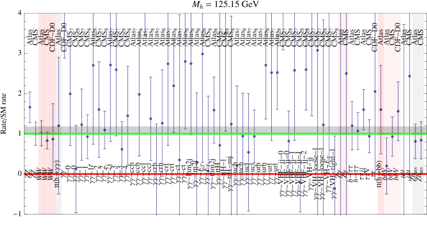 |
The experimental collaborations report Higgs boson rates in units of the central value of the SM prediction. Their results could be fully encoded in a likelihood , but only a limited amount of information is reported by the experiments. Often the experimental collaborations report the measured rates as : we use the results in this form whenever available. Sometimes collaborations only report the upper bounds on rates at 95% C.L., , and the expected upper bound at C.L. in absence of a Higgs boson signal, , as function of the Higgs boson mass . Assuming that the has a Gaussian form in , these two experimental informations allow one to extract the mean and the standard deviation as and , where arises because confidence level corresponds to about 2 standard deviations [8].111A similar procedure was described by Azatov et al. in [7]. The is approximated as
| (1) |
where the sum runs over all measured Higgs boson rates .
The theoretical uncertainties on the Higgs production cross sections start to be non-negligible and affect the observed rates in a correlated way.222 Note that the size of the theory uncertainty depends on the applied cuts, and that the scaling of the production cross section to yield the best-fit value relative to the theoretical central value may be different for very different sets of selection cuts (due to the QCD and PDF uncertainties). We take into account such correlations in the following way. We subtract from the total uncertainty the theoretical component due to the uncertainty in the production cross sections, obtaining the purely experimental uncertainty, . The theoretical error is reinserted by defining a which depends on the production cross sections ,
| (2) |
and marginalising it with respect to the free parameters , constrained to have a central value and an uncertainty given e.g. at by [10]
| (3) |
See also [38]. We neglect the relatively small uncertainties on the SM theoretical predictions for Higgs branching ratios, dominated by a uncertainty on the width.
We summarise all data in fig. 1 together with their error-bars. The grey band shows the range for the naive weighted average of all rates: . It lies along the SM prediction of 1 (horizontal green line) and, performing a naive average with Gaussian errors, it is almost 10 away from 0 (the horizontal red line is the background-only rate expected in the absence of a Higgs boson).
3 Reconstructing the Higgs mass
The CMS and ATLAS collaborations reported measurements of the pole Higgs mass obtained as the position of the peaks observed in the invariant mass of the and distributions. Averaging the results summarised in table 1 we find
| (4) |
The measurements are mutually compatible, and the uncertainty is small enough that in the subsequent fits to rates we can fix to its combined best-fit value. We combined all uncertainties in quadrature, using the standard Gaussian error propagation and neglecting correlations among systematic uncertainties. The averages within each experiment agree with those reported by the experiments.
We here discuss how the Higgs mass can be independently measured, with a larger uncertainty, by requiring that the measured rates agree with their SM predictions within their uncertainties. Such predictions have a dependence on the Higgs mass that, around 125 GeV, can be approximated as
| (5) |
In table 2 we list the values of the coefficients and of the measured rates for the various processes averaging all experiments, as well as the Higgs mass indirectly derived from such rates. We see that the single best indirect determination of comes from the rates, that presently have no sensitivity to if one wants to measure it from a mass peak. We see that best indirect determinations of comes from the rates (which presently have no sensitivity to if one wants to measure it from a mass peak) and from . On the other hand, the signal that offers the best peak measurement of has very little indirect sensitivity to , because the rate happens to have a weak dependence on . Averaging over all channels we find
| (6) |
which is compatible with the determination of the pole Higgs mass obtained in a model-independent way from the positions of the peaks.
4 The universal Higgs fit
We perform the most generic fit in terms of a particle with couplings to pairs of equal to in units of the SM Higgs coupling.
This means, for example, that the coupling to the top is given by , where in the SM and (from the measurement of the Fermi constant [42]) is the Higgs vacuum expectation value. Similarly, the coupling is assumed to be times its SM prediction. In the SM this couplings first arises at one loop level. Experiments are starting to probe also the and the effective couplings, so that also the corresponding and parameters will start to be measured. This discussion can be summarized by the following effective Lagrangian:
| (7) | |||||
The various SM loop coefficients are summarised in appendix A. This Lagrangian is often written in a less intuitive but practically equivalent form by either using -invariant effective operators, or assuming that the Higgs is the pseudo-Goldstone boson of a spontaneously broken global symmetry and writing its chiral effective theory [7]. We do not consider a modified Higgs coupling to charm quarks, given that decays at LHC are hidden by the QCD background. While we cannot exclude that new physics affects much more than all other Higgs properties, for simplicity we proceed by discarding this possibility.
Furthermore, we take into account the possibility of Higgs decays into invisible particles , such as Dark Matter or neutrinos [43], with branching ratio . In almost all measured rates (with the exception of the last data-point in fig. 1: the direct measurement of the invisible Higgs width) is equivalent to a common reduction of all the other Higgs couplings, , such that is indirectly probed by data [8]. The only observable that directly probes an invisible Higgs width is the rate measured by ATLAS [44] and CMS [45], which implies
| (8) |
Any possible new-physics model can be described as specific values of the parameters. Several examples are provided in section 5.
Following the procedure described in the previous section, we approximatively extract from data the function
| (9) |
which describes all the information contained in Higgs data. We find at the best fit (69 data points, 10 free parameters), marginally better than the SM fit, (no free parameters).
 |
4.1 Universal fit to small new physics effects
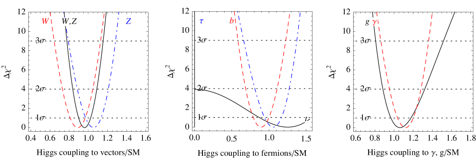
The universal of eq. (9) has a too complicated form to be reported analytically, and depends on too many variables to be reported in numerical form, such as plots or tables. For these reasons, previous analyses [7, 8, 9] focused on particular BSM models with a reduced number of parameters. For example, fig. 2 shows the fit as function of each , setting all others to their SM values of unity: we see that the are approximately parabolic.
We here observe that Higgs data are converging towards the SM predictions with small errors, thereby it is time to start making the approximation
| (10) |
and BR. The observable rates are computed at first order in , and consequently the is expanded up to second order in . As well known, this Gaussian approximation is a great simplification; for example marginalisations over nuisance parameters just becomes minimisation, which preserves the Gaussian form. Fig. 2 suggests that this approximation already seems reasonably good, particularly in the range of 1 or 2 standard deviations form the central value.
For LHC at the main observables are approximated as
| (11) |
where these expressions have been obtained by performing a first-order Taylor expansion in all the parameters of the full non-linear expressions. For all observables but the last one, we have assumed the total Higgs production cross section. When fitting the many real observables, we take into account the relative contribution of each production cross section, as determined by experimental cuts. For we here considered the gluon fusion production channel, and this makes the coefficients of somehow different from the other channels. The full can now be reported in a simple form. Indeed the is a quadratic function of the , and it is usually written as
| (12) |
in terms of the mean values of each parameter , of its error and in terms of the correlation matrix . We believe that this is the most useful form in which experimental collaborations could report their results. From our approximated analysis of LHC and Tevatron [14] data we obtain:
| (13) |
We have not reported the central value of , of and of because they presently are known only up to uncertainties much larger than 1. Future searches for production, for and for will improve the situation.
In many models the Higgs couplings to vectors satisfy , because of invariance. Furthermore, in many models LEP precision data force and to be very close to 0. This restriction can of course be implemented by just setting these parameters to be equal or vanishing in the quadratic .
Since the uncertainties on the parameters are now smaller then 1, the universal approximation starts to be accurate. In the next sections, where we analyze several specific models, we will systematically compare our full numerical fit (plotting best fit regions in yellow with continuous contours at the 90 and 99% C.L.) with the universal approximation (best fit ellipsoidal regions in gray with dotted contours, at the same confidence levels).
5 Model-dependent Higgs fits
|
5.1 Higgs production cross sections
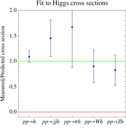
Assuming the SM predictions for Higgs decay fractions, we extract from the data the Higgs production cross sections. Given that measured rates of various exclusive and inclusive Higgs channels agree with their SM predictions, we find that production cross sections also agree with SM predictions, as shown in the left panel of fig. 3. As expected, the most precisely probed cross section is the dominant one, . At the opposite extremum is still largely unknown. The uncertainties on the reconstructed cross sections are correlated, although we do not report the correlation matrix.
|
5.2 Higgs couplings
We here extract from data the Higgs boson couplings to vectors and fermions, assuming that only the SM particles contribute to the loops. This amounts to restricting the universal fit in terms of the parameters by setting the parameters for loop couplings to
| (14) |
These numerical expressions are obtained by rescaling the expressions for the SM loops summarised in appendix A. In particular, the loop (rescaled by ) and the top loop (rescaled by ) contribute to with a negative interference.
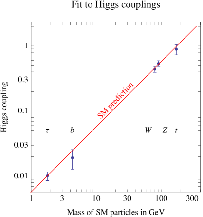
Under this assumption the top coupling of the Higgs, , becomes indirectly probed via the loop effects. The fit to the couplings is shown in fig. 3b and agrees with the SM predictions (diagonal line), signalling that the new boson really is the Higgs. The correlation matrix can be immediately obtained by inserting eq. (14) into the universal of eq. (12).
We allow the SM prediction to vary in position and slope by assuming that the Higgs couplings to particles with mass are given by . Taking into account all correlations, we find that data imply parameters and close to the SM prediction of (diagonal line in fig. 3b):
| (15) |
with a correlation.
5.3 Composite Higgs models
Models where the Higgs is composite often assume the further restriction, in addition to eq. (14), of a common rescaling with respect to their SM values of the Higgs boson couplings to the bosons and a common rescaling of the Higgs boson couplings to all fermions. These rescalings are usually denoted as and , respectively:
| (16) |
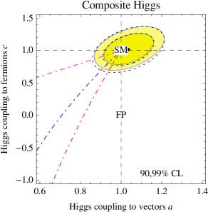
The resulting fit is shown in the left panel of fig. 4. We see that our approximated universal fit (dotted contours) reproduces very well our full fit (continuous contours). The best fit converged towards the SM; in particular data now disfavour the solution with which appeared in previous fits. Similar fits by the ATLAS and CMS collaborations are given in [46]. The CMS result is similar to ours, while ATLAS has , due to their larger rates, which is compatible with our result at level.
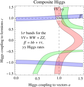
The reason is visualised in the middle panel of fig. 4, where we show the bands favoured by the overall rates for Higgs decay into heavy vectors ( and , that get affected in the same way within the model assumptions), into fermions ( and , that get affected in the same way within the model assumptions) and into . We see that these bands only cross around the SM point, . The full fit to all exclusive rates contains more information than this simplified fit.
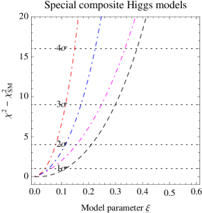
In the right panel of fig. 4 we show the full restricted along the trajectories in the plane (plotted in the left panel) predicted by simple composite pseudo-Goldstone Higgs models in terms of the parameter , where is the scale of global symmetry breaking [47], MeV.
|
|
 |
 |
 |
5.4 New physics only in the loop processes
We assume here that only the loop processes are modified with respect to the SM predictions, summarized in appendix A. This amounts to restricting our universal fit settings
| (17) |
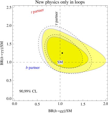
with BR and . The latter assumption is at present justified because of the large experimental error in the rate, even though in general new physics in the loop processes would induce deviation from unity in both and . The result is shown in the left panel of fig. 5, in the form of a fit to the ratios of and with respect to the SM. One can see that the SM is well within the contour. The analogous ATLAS result [46] is instead barely compatible with the SM at level because they only fit ATLAS data, where rates have a central value above the SM. The universal fit approximates the full fit reasonably well. The dashed trajectories show the loop effect due to extra scalar particles with the same quantum numbers of the top (red), of the bottom (blue), of the tau (vertical black line). The explicit expressions for the contribution of scalar, fermion and vector particles running in the loop can be found in appendix A. Note that any additional colorless but electrically charged particle would lead to the same trajectory obtained for the scalar partner of the .
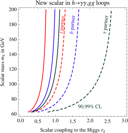
To better investigate the constraints on a possible new scalar , in the right panel of fig. 5 we show the upper bound, as function of the scalar mass , on the scalar coupling to the Higgs boson, defined by the coupling
| (18) |
The resulting loop effects are summarised in appendix A. The solid and dashed curves in fig. 5b are respectively the upper bounds at (solid) and (dashed) C.L. More stringent limits are obtained on the top and bottom partners than on the partner.
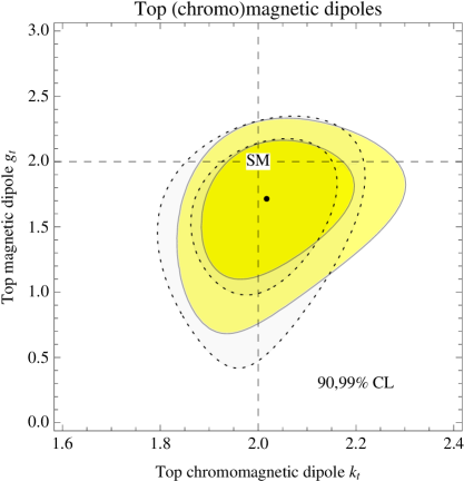
One can also use the universal fit with the assumption of eq. (17) to derive indirect constraints on the top quark magnetic () and chromomagnetic () dipole moments [48, 49], which in the SM are expected to be respectively and . Allowing and to vary freely, the and amplitudes are modified with respect to the SM as:
| (19) |
where the quantities and are defined in eq. (35) of the Appendix. Numerically we have and . Fig. 6 shows the and C.L. allowed regions for and . The uncertainty on is comparable to the one from its direct measurements at the LHC and the Tevatron as combined in [50], while the one for is even smaller. The conversion from the results of [50] is done in [48] for , giving , and in [49] for , giving at C.L.
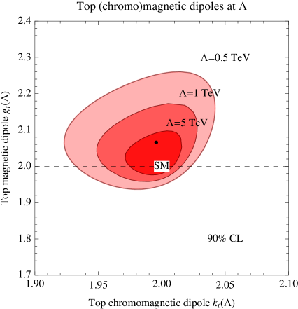
Eq. (19) was computed by [48, 49] at the weak scale, in the phase with broken electroweak symmetry. An analogous computation was performed in [51], promoting the dipoles to full -invariant effective operators with a non-renormalizable dimension , suppressed by a factor , being the cutoff of the theory. The result [51] is that the dipole operators before electroweak symmetry breaking contribute, via RGE mixing, to other one-loop suppressed operators affecting the and decay rates [52]. Finite parts are not computed. Because of the RGE running from down to , the effect is proportional to , differently from eq. (19). Using the operator mixing result of [51] and parametrizing the dipole operators at via quantities analogous to and but defined at , the decay rates [52] can be written as
| (20) |
where the quantity is defined in eq. (35) of the Appendix. Numerically . Repeating our fit, we obtain similar constraints as illustrated in the right panel of fig. 6, for representative values of the cutoff.
5.5 Models with two Higgs doublets
There are four types of two Higgs doublets models (2HDM) where tree-level flavour-changing neutral currents (FCNCs) are forbidden by a symmetry [53] and both doublets and get a vacuum expectation value:
- •
- •
-
•
type X (lepton-specific or leptophilic) where couples only to quarks and couples only to leptons;
-
•
type Y (flipped) [57], where couples to up-type quarks and to down-type quarks, and (contrary to the type II HDM) leptons couple to .
For an extensive review see [58] and for some previous fits see [59]. The modification to Yukawa couplings to up-type and down-type quarks and leptons in the four 2HDMs are:
| Type I | Type II | Type X (lepton-specific) | Type Y (flipped) | |
|---|---|---|---|---|
As usual, is the ratio of the VEVs of the two doublets and is the mixing angle of the CP-even mass eigenstates. The SM limit corresponds to . In all of the models the vector couplings are also modified as
| (21) |
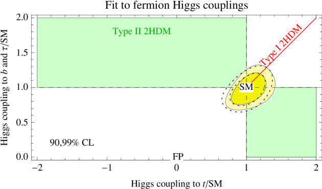
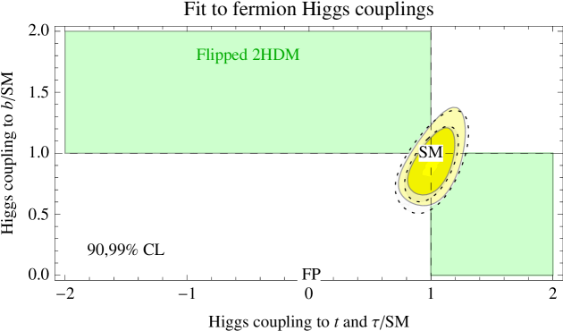
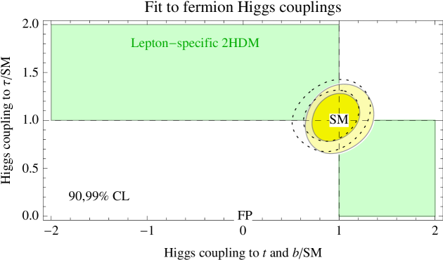
The results of our fits are presented in fig. 7 in terms of the fermion couplings , restricted by the 2HDM models to lie within the green regions. (We do not show the region for which is allowed since the measurements have no sensitivity to the signs of these couplings.) We find that in each case, it is that dominates the fit and the bottom contributions to gluon fusion and are negligible.The effect of the charged Higgs boson in the loop is neglected.
The type II 2HDM (upper panel) allows for independent modification of the coupling , and for a common modification of the and couplings, . The former is predicted be reduced and the latter enhanced by the model. The modification of eq. (21) of the vector couplings can be equivalently written as , showing that it is a small second order effect. In this model a negative Yukawa coupling is still allowed at slightly more than 99% CL. The red line in the same panel shows the parameter space allowed by type I 2HDM, where all the couplings scale uniformly.
In the flipped 2HDM (middle panel) the Yukawa coupling changes in the same way as the coupling and the region with negative coupling is disfavoured by data. Finally, in the leptophilic 2HDM (lower panel) the and couplings vary in the same way, while the coupling is independent.
The universal fit provides a reasonable approximation to the full fit in all 2HD models.
5.6 Supersymmetry
Supersymmetry can affect Higgs physics in many different ways, such that it is difficult to make general statements. We here focus on the two most plausible effects:
-
•
The stop squark loop affect the rates. Given that the stop has the same gauge quantum numbers of the top, such effects are correlated and equivalent to a modification of the Higgs coupling to the top (as long as it is not directly measured via the production cross section) by an amount given by
(22) in the limit of heavy stop masses, . Notice that can be enhanced or reduced with respect to one, depending on the latter mixing term.
-
•
The type II 2HDM structure of supersymmetric models modifies at tree-level the Higgs couplings, as already discussed in section 5.5.
All of this amounts to specialise the universal inserting the following values of its parameters
| (23) |
Furthermore, the parameters relative to loop processes are fixed as in eq. (14). We trade the parameter (mass mixing between Higgses) for the pseudo-scalar Higgs mass using
| (24) |
Finally, we assume a large , as motivated by the observed value of the Higgs mass (a large amplifies the stop contribution to the Higgs mass). The left panel of fig. 8 shows the resulting fit. Once again, the universal fit is an adequate approximation of the full fit. Of course, supersymmetry can manifest in extra ways not considered here, e.g. very light staus or charginos could enhance [60].
 
|
5.7 Data prefer the Higgs to the dilaton
As another example of a model where both the tree-level and the loop level Higgs couplings are modified, we consider the dilaton. The dilaton is an hypothetical particle , that, like the Higgs, couples to SM particles with strength proportional to their masses [61]. More precisely the dilaton has a coupling to the trace of the energy-momentum tensor , suppressed by some unknown scale :
| (25) |
The dilaton couplings to and differ from the corresponding Higgs boson couplings, because eq. (25) contains the latter two quantum terms, that are present in because scale invariance is anomalous and broken at quantum level by the running of the couplings. Indeed and are the -function coefficients of the strong and electromagnetic gauge couplings. In the SM they have the explicit values and : we call ‘pure dilaton’ this special model, which gives a significant enhancement of .
Models where a dilaton arises usually often contain also new light particles, such that and can differ from their SM values. Thereby we perform a generic fit where and are free parameters in addition to . Then, our universal fit is adapted to the case of the generic dilaton by setting
| (26) |
where .
In our previous analyses [8, 9], the dilaton gave fits of comparable quality to the SM Higgs, despite the significantly different predictions of the dilaton: enhanced rates and reduced vector boson fusion rates. The first feature is no longer favoured by data, and the second feature is now disfavoured: so we find that present data prefer the Higgs to the ‘pure dilaton’ at about level. We then consider the generic dilaton, showing in fig. 8b that the allowed part of its parameters space is the one where it mimics the Higgs, possibly up to a sign difference in and/or . The linear couplings of the dilaton in eq. (25) become identical to those of the SM Higgs in the limit and . This situation is not easily realisable in models, given that adding extra charged particles increases rather than reducing it; one needs to subtract particles by e.g. assuming that that 3rd generation particles are composite [64].
The universal approximation works reasonably well, although it cannot reproduce these disjoint solutions.
|
5.8 Higgs boson invisible width
Next, we allow for a Higgs boson invisible width, for example into Dark Matter (this does not comprise undetectable decays into known physics, such as Higgs to light jets).444 Note that such decays are only undetectable at hadron colliders due to large QCD backgrounds and trigger problems, but could be detected at an collider in the production mode. We perform two fits.
-
1.
In the first fit, the invisible Higgs width is the only new physics. We find (blue curves in fig. 9a) that present data imply . The one-sided upper bound, computed restricting to , is
(27) -
2.
In addition to the invisible width we also allow for non-standard values of and , finding a weaker constraint on BRinv (red curves in fig. 9a)
(28) The reason is that an enhanced production rate can partially compensate for an invisible Higgs width, but a full compensation would be possible only by enhancing all production rates by the same amount. The Higgs coupling to vectors is independently measured to agree with SM predictions from electroweak precision data.
Notice that the main constraint for BRinv does not come from the direct search for (included in our data-set) but from the global fit [8, 62].
5.9 Dark Matter models
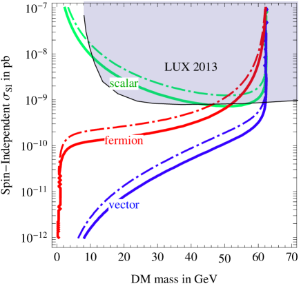
The invisible Higgs boson decay width [62] constrains Dark Matter (DM) candidates with mass below . The Higgs sector of the SM allows for a direct coupling to particles of a hidden sector. If the latter are stable and interact weakly with the SM sector, they could represent viable Dark Matter (DM) candidates. If DM particles have mass below , the Higgs boson can thus decay into a pair of DM particles, which would escape detection. Invisible Higgs decays are constrained by the fact that the ATLAS and CMS Higgs rates are compatible with the predictions of the SM Higgs boson. The experimental bound on BRinv can be used to constrain the DM mass and its elastic cross section on nucleons probed in direct detection experiments, as illustrated for instance in [63], where DM is assumed to be either a scalar , or a Majorana fermion or a vector coupled to the Higgs as
| (29) |
The partial Higgs decay width into dark matter and the spin-independent -proton elastic cross section can be calculated in terms of the parameters of the above Lagrangian. Both are proportional to the square of the DM-Higgs coupling, so that the ratio depends only on the the unknown DM mass and on the known masses and couplings of the relevant SM particles (see for instance the expressions provided in [63]).
This allows us to relate the invisible Higgs branching fraction to the DM direct detection cross section:
| (30) |
where is the total Higgs decay width into all SM particles, that we fix to its SM prediction. For a given DM mass, an upper bound on the Higgs invisible branching fraction implies an upper bound on the DM scattering cross section on nucleons. The relation between the invisible branching fraction and the direct detection cross section strongly depends on the spinorial nature of the DM particle, in particular, the strongest (weakest) bound is derived in the vectorial (scalar) case.
Imposing the upper bounds on BRinv derived in section 5.8, fig. 9 shows the corresponding upper limits on the spin-independent DM cross section on nucleons as a function of the DM mass, in the case of scalar (green), Majorana fermion (red) and vector (blue) DM candidates.
In all cases, the derived bounds are stronger than the direct one from LUX2013 as long as the mass of is lighter than . This conclusion does not rely on the assumption that DM is a thermal relic that reproduces the observed cosmological DM abundance. The limit on crucially depends on the assumption that DM directly couples to the Higgs. Larger values of remain possible in different models, where DM couples to the or directly to nucleons via loops of supersymmetric or other particles.
6 Discussion and Conclusions
The LHC experiments reported their measurements of Higgs boson properties at the Moriond 2013 conferences, based on the full collected luminosity during 2011 and 2012. At the same time, Tevatron reported their final Higgs results. With the crucial inclusion of the full CMS data (missing in previous analyses), at this stage all main Higgs results from Tevatron and from the first phase of LHC have been basically presented. Those results will drive our understanding of particle physics, until new 13 TeV LHC data will be available.
Motivated by these results, we have performed a state-of-the-art global fit to Higgs boson data, including all sub-categories studied by the experimental collaborations, for a total of 56 experimental inputs, as summarised in fig. 1. We found that the average Higgs rate is in SM units, supporting the SM Higgs boson hypothesis. The Higgs boson mass is usually determined from the peaks in the invariant mass distribution of and . We performed the first measurement of the Higgs boson mass from the rates, finding that the two determinations are compatible:
| (31) |
The LHC physics program has been successful: with only /fb of data per experiment the Higgs boson has been discovered and several of its properties determined within precision. We are now entering into the era of precision Higgs physics — deviations from the SM due to new physics no longer can dominate the data. This observation allowed us to propose a ‘universal’ form in which experiments could report their results allowing theorists to easily test any desired model. The new assumption that makes possible this significant simplification is that new physics is a small correction to the SM. While we used all publicly available data to present our own global combination in ‘universal’ form in eq. (13), we stress that only the experimental collaborations can perform a fully precise analysis, for example including the correlations among experimental uncertainties.
We studied several new physics scenarios beyond the SM. We determined from data the production cross sections (assuming standard Higgs decays) and the Higgs decays widths (assuming standard productions), finding that they lie along the SM predictions. In a more general context, we allowed all possible Higgs boson couplings to any SM particle to deviate from its SM value, finding that couplings to the must lie around their SM predictions up to uncertainties of about (see fig. 3b). In particular, non-standard Higgs boson couplings to vectors, predicted by composite Higgs models, are most stringently constrained. The scenario of negative Higgs coupling to fermions (‘dysfermiophilia’) that gave the best fit with early LHC data is now disfavoured at more than .
We considered various specific new physics models: new scalars, 2HDM, supersymmetry, dilaton, composite Higgs, invisible Higgs decays, possibly into Dark Matter particles, anomalous couplings of the top, etc. The results of those fits are presented in numerous figures throughout the paper. Qualitatively, all reach the same conclusions:
-
i)
best fit regions lie along SM predictions, imposing constraints on new physics;
-
ii)
our simple universal fit is a reasonable approximation to the full fit.
In particular we find that, with the latest data, the dilaton alternative to the Higgs is now excluded at , with the exception of the special non-minimal dilaton tuned to exactly reproduce the Higgs (section 5.7).
We will update this paper when future results become available.
Acknowledgement
This work was supported by the ESF grants 8943, MTT8, MTT59, MTT60, MJD140 by the recurrent financing SF0690030s09 project and by the European Union through the European Regional Development Fund. The work of P. P. G. has been partially funded by the “Fondazione A. della Riccia”. This work was supported in part by the European Programme PITN-GA-2009-23792 (UNILHC).
Appendix A New physics contributions to loop processes
The coefficients in the second line of eq. (7) arise at one-loop. They are obtained by summing the contributions of all scalars () fermions () and vectors () that couple to the Higgs as in eq. (29). The explicit expressions for the loop effects are [66]:
| (32) | |||
where for each particle , , is the number of colors, is the Casimir of the color representation (Tr), and the loop functions are
| (33) | |||||
| (34) |
with such that in the limit (heavy -particle).
In particular, in the SM, the coupling is dominated by the top loop, and the coupling arise from the sum of the top and boson loops:
| (35) |
Beyond the SM (BSM) physics affects the parameters and as
| (36) |
For example, additional scalar particles with the same quantum numbers of a stop, sbottom and stau respectively contribute to and to as:
| (37) |
References
- [1] ATLAS Collaboration, Phys. Lett. B 716 (2012) 1 [arXiv:1207.7214].
- [2] CMS Collaboration, Phys. Lett. B 716 (2012) 30 [arXiv:1207.7235].
- [3] F. Englert and R. Brout, Phys. Rev. Lett. 13, 321 (1964).
- [4] P. W. Higgs, Phys. Lett. 12 (1964) 132.
- [5] P. W. Higgs, Phys. Rev. Lett. 13, 508 (1964).
- [6] G. S. Guralnik, C. R. Hagen and T. W. B. Kibble, Phys. Rev. Lett. 13, 585 (1964).
- [7] D. Carmi, A. Falkowski, E. Kuflik and T. Volansky, JHEP 1207 (2012) 136, arXiv:1202.3144. A. Azatov, R. Contino and J. Galloway, JHEP 1204 (2012) 127, arXiv:1202.3415. J. R. Espinosa, C. Grojean, M. Muhlleitner and M. Trott, JHEP 1205 (2012) 097, arXiv:1202.3697. T. Li, X. Wan, Y. Wang and S. Zhu, JHEP 1209 (2012) 086, arXiv:1203.5083. J. Ellis and T. You, JHEP 1206 (2012) 140, arXiv:1204.0464. A. Azatov, R. Contino, D. Del Re, J. Galloway, M. Grassi and S. Rahatlou, JHEP 1206 (2012) 134, [arXiv:1204.4817]. M. Klute, R. Lafaye, T. Plehn, M. Rauch and D. Zerwas, Phys. Rev. Lett. 109 (2012) 101801, arXiv:1205.2699; A. Azatov, S. Chang, N. Craig and J. Galloway, Phys. Rev. D 86 (2012) 075033 [arXiv:1206.1058]. I. Low, J. Lykken and G. Shaughnessy, Phys. Rev. D 86 (2012) 093012 [arXiv:1207.1093]. T. Corbett, O. J. P. Eboli, J. Gonzalez-Fraile and M. C. Gonzalez-Garcia, Phys. Rev. D 86 (2012) 075013 [arXiv:1207.1344]. M. R. Buckley and D. Hooper, Phys. Rev. D 86 (2012) 075008 [arXiv:1207.1445]. M. Montull and F. Riva, JHEP 1211 (2012) 018 [arXiv:1207.1716]. J. R. Espinosa, C. Grojean, M. Muhlleitner and M. Trott, JHEP 1212 (2012) 045, arXiv:1207.1717. D. Carmi, A. Falkowski, E. Kuflik, T. Volansky and J. Zupan, JHEP 1210 (2012) 196, [arXiv:1207.1718]. S. Banerjee, S. Mukhopadhyay and B. Mukhopadhyaya, JHEP 1210 (2012) 062, [arXiv:1207.3588]. D. Bertolini and M. McCullough, JHEP 1212 (2012) 118, [arXiv:1207.4209]. F. Bonnet, T. Ota, M. Rauch and W. Winter, Phys. Rev. D 86 (2012) 093014, [arXiv:1207.4599]. T. Plehn and M. Rauch, Europhys. Lett. 100 (2012) 11002, [arXiv:1207.6108]. J. R. Espinosa, C. Grojean, V. Sanz and M. Trott, JHEP 1212 (2012) 077, arXiv:1207.7355. A. Djouadi, Eur. Phys. J. C73 (2013) 2498, arXiv:1208.3436. L. Maiani, A. D. Polosa, V. Riquer, Phys. Lett. B718 (2012) 465-468, arXiv:1209.4816. G. Cacciapaglia, A. Deandrea, G. D. La Rochelle and J. -B. Flament, JHEP 1303 (2013) 029, arXiv:1210.8120. G. Moreau, Phys. Rev. D87 (2013) 015027, arXiv:1210.3977. G. Belanger, B. Dumont, U. Ellwanger, J. F. Gunion and S. Kraml, JHEP 1302 (2013) 053 E. Masso and V. Sanz, arXiv:1211.1320. T. Corbett, O. J. P. Eboli, J. Gonzalez-Fraile and M. C. Gonzalez-Garcia, Phys. Rev. D 87 (2013) 015022 [ arXiv:1211.4580]. [arXiv:1212.5244]. C. Cheung, S. D. McDermott and K. M. Zurek, JHEP 1304 (2013) 074, arXiv:1302.0314. K. Cheung, J. S. Lee and P. -Y. Tseng, JHEP 1305 (2013) 134, arXiv:1302.3794. A. Falkowski, F. Riva and A. Urbano, JHEP 1311 (2013) 111, arXiv:1303.1812.
- [8] P. P. Giardino, K. Kannike, M. Raidal and A. Strumia, JHEP 1206 (2012) 117 [arXiv:1203.4254].
- [9] P. P. Giardino, K. Kannike, M. Raidal and A. Strumia, Phys. Lett. B718 (2012) 469-474 [arXiv:1207.1347].
- [10] LHC Higgs Cross Section Working Group, arXiv:1101.0593 (Recommended values on SM Higgs XS at 7 TeV and SM Higgs production cross sections at TeV (2012 update)), arXiv:1201.3084, arXiv:1307.1347. (Branching Ratios and Partial-Decay Widths).
- [11] Guillelmo Gomez-Ceballos, CMS Collaboration, Talk at the Moriond 2013 EW session.
- [12] Fabrice Hubaut, ATLAS Collaboration, Talk at the Moriond 2013 EW session. Eleni Mountricha, ATLAS Collaboration, Talk at the Moriond 2013 QCD session.
- [13] Valentina Dutta, CMS Collaboration, Talk at the Moriond 2013 EW session. Victoria Martin, ATLAS Collaboration, Talk at the Moriond 2013 EW session.
- [14] T. Aaltonen et al. [CDF and D0 Collaborations], Phys. Rev. D 88 (2013) 052014 [arXiv:1303.6346 [hep-ex]].
- [15] CMS Collaboration, CMS-PAS-HIG-13-001. ATLAS Collaboration, ATLAS-CONF-2013-012.
- [16] S. Chatrchyan et al. [CMS Collaboration], [arXiv:1312.5353 [hep-ex] ]. G. Aad et al. [ATLAS Collaboration], Phys. Lett. B 726 (2013) 88 [arXiv:1307.1427 [hep-ex]].
- [17] CMS Collaboration, CMS-PAS-HIG-13-003. S. Chatrchyan et al. [CMS Collaboration], arXiv:1312.1129 [hep-ex]. ATLAS Collaboration, ATLAS-CONF-2013-030.
- [18] CMS Collaboration, CMS-PAS-HIG-13-004. ATLAS Collaboration, ATLAS-CONF-2013-108.
- [19] Mónica Vázquez Acosta, CMS Collaboration, Talk given at CERN.
- [20] S. Chatrchyan et al. [CMS Collaboration], arXiv:1310.3687 [hep-ex]. ATLAS Collaboration, ATLAS-CONF-2013-079.
- [21] David Lopez Mateos, ATLAS Collaboration, talk given at the EPS HEP 2013 conference.
- [22] ATLAS Collaboration, ATLAS-CONF-2013-010.
- [23] S. Chatrchyan et al. [CMS Collaboration], Phys. Lett. B 726 (2013) 587 [arXiv:1307.5515]. ATLAS Collaboration, ATLAS-CONF-2013-009.
- [24] CMS Collaboration, CMS-PAS-HIG-13-009.
- [25] Mingshui Shen, CMS Collaboration, Talk at the Moriond 2013 EW session. Bruno Mansoulie, CMS Collaboration, Talk at the Moriond 2013 EW session. ATLAS Collaboration, ATLAS-CONF-2013-014.
- [26] Eve Le Menedeu, ATLAS Collaboration, Talk at the Moriond 2013 EW session.
- [27] Sandrine Laplace, ATLAS Collaboration, Talk at the ICHEP 2014.
- [28] Gabriella Sciolla, ATLAS Collaboration, Talk at the ICHEP 2014.
- [29] G. Aad et al. [ ATLAS Collaboration], arXiv:1406.7663 [hep-ex].
- [30] Elizaveta Shabalina, ATLAS Collaboration, Talk at the ICHEP 2014. ATLAS Collaboration, ATLAS-CONF-2014-043.
- [31] Matthew Kenzie, CMS Collaboration, Talk at the ICHEP 2014. CMS Collaboration, arXiv:1407.0558.
- [32] Adish Vartak, CMS Collaboration, Talk at the ICHEP 2014.
- [33] Pietro Govoni, CMS Collaboration, Talk at the ICHEP 2014.
- [34] Jan Steggemann, CMS Collaboration, Talk at the ICHEP 2014.
- [35] Michail Bachtis, CMS Collaboration, Talk given at CERN in July 2014.
- [36] Sani Matteo, CMS Collaboration, Talk at the ICHEP 2014.
- [37] Robert Harrington, ATLAS Collaboration, Talk at the ICHEP 2014.
- [38] M. Duhrssen, S. Heinemeyer, H. Logan, D. Rainwater, G. Weiglein and D. Zeppenfeld, Phys. Rev. D 70 (2004) 113009 [hep-ph/0406323].
- [39] ATLAS Collaboration, ATLAS-CONF-2013-014.
- [40] CMS Collaboration, CMS-PAS-HIG-13-005.
- [41] LHC Higgs Cross Section Working Group Collaboration, arXiv:1209.0040.
- [42] MuLan Collaboration, Phys. Rev. D 87 (2013) 5, 052003 [arXiv:1211.0960].
- [43] K. Belotsky, D. Fargion, M. Khlopov, R. Konoplich and K. Shibaev, Phys. Rev. D 68 (2003) 054027 [arXiv:hep-ph/0210153].
- [44] ATLAS Collaboration, ATLAS-CONF-2013-011 See also A. Djouadi, A. Falkowski, Y. Mambrini and J. Quevillon, arXiv:1205.3169.
- [45] CMS Collaboration, CMS-PAS-HIG-13-018.
- [46] ATLAS Collaboration, ATLAS-CONF-2013-034. CMS Collaboration, CMS-PAS-HIG-13-005.
- [47] G. F. Giudice, C. Grojean, A. Pomarol and R. Rattazzi, JHEP 0706 (2007) 045 [arXiv:hep-ph/0703164]. A. Pomarol and F. Riva, JHEP 1208 (2012) 135 [arXiv:1205.6434].
- [48] L. Labun and J. Rafelski, arXiv:1209.1046.
- [49] L. Labun and J. Rafelski, arXiv:1210.3150.
- [50] J. F. Kamenik, M. Papucci and A. Weiler, Phys. Rev. D 85 (2012) 071501 [arXiv:1107.3143].
- [51] J. Elias-Miro, J. R. Espinosa, E. Masso, A. Pomarol and , arXiv:1302.5661. See also: C. Degrande, J. M. Gerard, C. Grojean, F. Maltoni, G. Servant and , JHEP 1207 (2012) 036 [Erratum-ibid. 1303 (2013) 032] [arXiv:1205.1065]. R. Contino, M. Ghezzi, C. Grojean, M. Muhlleitner and M. Spira, arXiv:1303.3876.
- [52] A. V. Manohar and M. B. Wise, Phys. Lett. B 636 (2006) 107 [arXiv:hep-ph/0601212].
- [53] S. L. Glashow and S. Weinberg, Phys. Rev. D 15 (1977) 1958.
- [54] H. E. Haber, G. L. Kane and T. Sterling, Nucl. Phys. B 161 (1979) 493.
- [55] L. J. Hall and M. B. Wise, Nucl. Phys. B 187 (1981) 397.
- [56] J. F. Donoghue and L. F. Li, Phys. Rev. D 19 (1979) 945.
- [57] V. D. Barger, J. L. Hewett and R. J. N. Phillips, Phys. Rev. D 41 (1990) 3421. Y. Grossman, Nucl. Phys. B 426 (1994) 355 [hep-ph/9401311]. A. G. Akeroyd and W. J. Stirling, Nucl. Phys. B 447 (1995) 3. A. G. Akeroyd, Phys. Lett. B 377 (1996) 95 [hep-ph/9603445]. A. G. Akeroyd, J. Phys. G 24 (1998) 1983 [J. Phys. G G 24 (1998) 1983] [hep-ph/9803324]. M. Aoki, S. Kanemura, K. Tsumura and K. Yagyu, Phys. Rev. D 80 (2009) 015017 [arXiv:0902.4665].
- [58] G. C. Branco, P. M. Ferreira, L. Lavoura, M. N. Rebelo, M. Sher and J. P. Silva, Phys. Rept. 516 (2012) 1 [arXiv:1106.0034].
- [59] R. T. D’Agnolo, E. Kuflik and M. Zanetti, arXiv:1212.1165. A. Celis, V. Ilisie and A. Pich, arXiv:1302.4022.
- [60] M. Carena, I. Low and C. E. M. Wagner, arXiv:1206.1082. L. Wang and X. -F. Han, arXiv:1206.1673. W. -F. Chang, J. N. Ng and J. M. S. Wu, arXiv:1206.5047. N. Bonne and G. Moreau, arXiv:1206.3360. B. Bellazzini, C. Petersson and R. Torre, arXiv:1207.0803. J. Baglio, A. Djouadi and R. M. Godbole, arXiv:1207.1451. G. F. Giudice, P. Paradisi, A. Strumia and A. Strumia, JHEP 1210 (2012) 186 [arXiv:1207.6393].
- [61] L. Randall and R. Sundrum, Phys. Rev. Lett. 83 (1999) 3370. Y. Eshel, S. J. Lee, G. Perez and Y. Soreq, JHEP 1110 (2011) 015 [arXiv:1106.6218]; V. Barger and M. Ishida, arXiv:1110.6452. K. Cheung and T. -C. Yuan, Phys. Rev. Lett. 108 (2012) 141602 [arXiv:1112.4146].
- [62] J. R. Espinosa, M. Muhlleitner, C. Grojean and M. Trott, arXiv:1205.6790. G. Belanger, B. Dumont, U. Ellwanger, J. F. Gunion and S. Kraml, arXiv:1302.5694.
- [63] A. Djouadi, A. Falkowski, Y. Mambrini and J. Quevillon, arXiv:1205.3169.
- [64] B. Bellazzini et al., arXiv:1209.3299.
- [65] LUX Collaboration, arXiv:1310.8214.
- [66] For a recent review see A. Djouadi, Phys. Rept. 457 (2008) 1 [hep-ph/0503172].