Variation of the Diameter of the Sun as Measured by the Solar Disk Sextant (SDS)

Abstract

The balloon-borne Solar Disk Sextant (SDS) experiment has measured the angular size of the Sun on seven occasions spanning the years 1992 to 2011. The solar half-diameter – observed in a 100-nm wide passband centred at 615 nm – is found to vary over that period by up to 200 mas, while the typical estimated uncertainty of each measure is 20 mas. The diameter variation is not in phase with the solar activity cycle; thus, the measured diameter variation cannot be explained as an observational artefact of surface activity. Other possible instrument-related explanations for the observed variation are considered but found unlikely, leading us to conclude that the variation is real. The SDS is described here in detail, as is the complete analysis procedure necessary to calibrate the instrument and allow comparison of diameter measures across decades.

1 Introduction

Measuring the solar diameter (and its variations) has a long and controversial history with results highly inconsistent with each other, not only in absolute values, but also in trends with time. Detailed reviews of these efforts are presented in Djafer et al. (2008) and Thuillier et al. (2005, 2006) and will not be repeated here. More specifically, here we will only address direct measurements, as opposed to values derived from the analysis of historical data (e.g. duration of solar eclipses, timings of transits of Mercury, etc.). A summary compilation of radius measurements from 1660 to the present era (Pap et al. 2001) shows differences in excess of 2 arcsec, which persist to recent simultaneous measurements. See for instance Table 1 of Djafer et al. (2008), which summarizes such direct measurements, showing that they exhibit differences of up to 0.8 arcsec while claiming internal accuracy of a few tens of milli-arcseconds. The main conclusion of the paper by Djafer et al. was that measuring the solar diameter is a very difficult undertaking, and that the principal causes of the inconsistent results are the effects of the Earth’s atmosphere, differences in the definition of the limb edge, the spectral range of the measurements, and instrumental differences that cannot be independently calibrated with a precision higher than the expected variations.

On the more specific issue of variability, the results are even more extreme (Thuillier et al. 2005), varying from 1000 mas amplitude and in phase with solar activity (Noël 2004), to 200 mas and out of phase (Delmas & Laclare 2002, Egidi et al. 2006), to no significant change (Brown & Christensen-Dalsgaard 1998, Wittmann 2003, Penna et al. 2002, Kuhn et al. 2004).

Whereas differences of the results between the different diameter determinations can arise from the various edge definition algorithms, and the range of wavelength of measurements, the extreme differences in trends can only arise from atmospheric effects, and/or from the large instrumental effects produced by the extreme environment of Sun-pointing telescopes that do not have a system for internal scale calibration.

This is best illustrated by Noël (2004) where it is shown that concurrent measurements made with the same type of instrument (Danjon astrolabes) located at Calern, (France), Santiago, (Chile), and Rio de Janeiro (Brazil) not only show differences of up to $0.4^{\prime\prime}$, but also differ in trend with time. The Calern data exhibit an anticorrelation with the solar activity cycle, while the South American data show a positive correlation.

If we confine our discussion to space borne (or space-like) measurements, the atmospheric effects are removed, or greatly reduced, and what remains are the instrumental effects. This selection leaves only 5 experiments for which diameter measurements have been attempted: the MDI on SOHO, the HMI on SDO, RHESSI, the SODISM experiment on PICARD, and the SDS. Of those, only the SDS and SODISM have internal calibration capability. Because of the absence of such calibration, the RHESSI results only presented determinations of the solar oblateness, but not of the diameter (Fivian et al. 2008). This was based on the reasonable assumption that the instrumental scale would not change significantly during the short interval in which an instrumental rotation is performed. Angular diameter determinations with SOHO/MDI (Bush et al. 2010) find no discernible variation, although without an internal angular calibration these measurements must rely on other means of correcting significant long-term changes in the instrument. As with RHESSI, SDO/HMI has made observations sufficient to measure the solar oblateness (Fivian et al. 2012), although results of these measures have yet to appear. SDO has not been operating long enough to address the issue of long-term solar diameter variation. PICARD/SODISM (Thuillier et al. 2011, Assus et al. 2008) is still in a validation phase, and no results have been published to date. As a consequence, the only currently available results from instruments in a space-like environment and with internal calibration, are the SDS results presented here.

Because the SDS is balloon-borne, it can only be flown during periods when the high-velocity stratospheric winds change direction (twice per year) at which time, and for a few days, their velocity is low (the so called turnaround period). During turnaround we can have day-long flights and still remain within the range of control of the NASA/Columbia Scientific Balloon Facility (CSBF), the organization that operates these flights. Moreover, at the location of the CSBF base in Fort Sumner, New Mexico, turnaround occurs in early May and late September. At the spring turnaround, the Sun is too high in the sky, so that for several hours around local noon the Sun would be behind the balloon, and hours of observation would be lost. As a consequence, flights are not recommended at that time. Hence, only fall flights are desirable. More precisely, since the SDS in the current gondola cannot tilt above 53^∘, those flights have to take place on September 25 or later.

Although we have flown the SDS eleven times, starting in the late 1980s, the instrumental configuration required to reach a precision of tens of milliarc sec (to be explained in Section 2) was only achieved starting with Flight 6, in 1992. As a consequence, this paper only presents the results of the seven flights since and including Flight 6.

We describe the SDS instrument and its operation in Sections 2 and 3, respectively. Section 4 details the data-analysis procedures and pipeline. Section 5 presents the diameter results and Section 6 discusses them, while Section 7 provides a concluding summary.

2 SDS Instrument

The current version of the SDS balloon borne instrument is a package that has been successfully flown several times on 12 - 29 Mcf (million cubic ft) balloons. The basic principle of the SDS instrument is the use of a mechanically and optically stable beam splitting wedge (BSW) as an angle reference to form a double image of the Sun separated by slightly more than its angular diameter. The constancy of the angle of the BSW is achieved by utilizing molecular contact fabrication techniques. It can be shown that by measuring the small distance between images, $d$, one can achieve the necessary accuracy much more easily than if one attempts to measure the full diameter directly. The level of dimensional stability required within the focal plane is relaxed as $d/D$, where $D$ is the distance between the centre of two solar images; in our case $d\sim 6$ mm and $D\sim 200$ mm. Figure 1 illustrates the measurement concept and the layout of the detectors in the SDS focal plane.

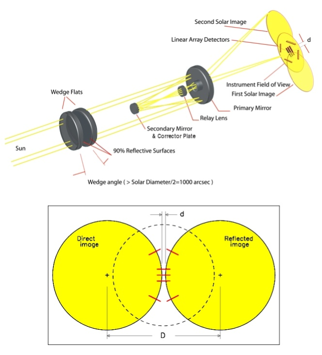
Figure 1: Upper: Optical layout of the SDS. The SDS is built around a ruggedized Questar telescope supplemented with a beam splitting wedge and a Barlow relay lens to increase the focal length. The beam splitting wedge produces a direct image and a reflected image that is offset by slightly more than the Sun’s diameter. The solar limb is measured along ten radials by seven linear-array CCDs mounted in the focal plane. Insert: Detail of the detector plane. The red line segments indicate the location of the CCDs; the dotted circle shows the approximate field of view. The solar diameter is determined by precise measurement of the disks’ separation, $D$, and gap, $d$.

This method also allows one to monitor and correct for instrument changes (e.g. focal length changes, etc.) in a straightforward way. Changes in any of the optical components downstream of the wedge will affect both images and can be calibrated out. The instrument consists of three basic items, the optical system, the assembly of linear-array detectors, and the electronics package mounted separately from the telescope. The accuracy of the SDS derives from the system design, which uses a single optical train to transfer the split solar images to the detectors.

In the current instrument, $F$ = 20.5 m, and $2W=1978.94^{\prime\prime}$. Further details of the instrumental properties are given in Sofia et al. (1991) and summarized in Table 1.

Table 1: SDS characteristics

focal length :	20.5 m
aperture :	12.7 cm
passband :	$\lambda_{o}$ = 615 nm, $\delta\lambda\sim$ 100 nm
pixel scale :	0.13 arcsec/pixel
wedge angle $\times$2 :	1978.94 arcsec

2.1 Optical system

The stability of the optics needed by this instrument is of the level commonly used in optical interferometry. For this reason, the balloon flight version currently utilizes similar techniques (molecular bonding) and materials (quartz and Zerodur). Thus, the optical system consists of the following components:

1. beam splitting wedge (BSW),

2. Cassegrain telescope,

3. relay lens, to achieve the required focal length, and

4. detector support.

2.1.1 Beam splitting wedge (BSW)

Because the wedge is the most critical element in the optical system, great care is taken with its design and manufacture. The wedge consists of two fused silica flats separated by an annular silica ring polished to an angle of about 1000 arcsec. Molecular contact bonding is used to hold the assembly in alignment. The surfaces are flat to 1/50 wave at 630 nm and have dielectric coatings to define the bandpass and reduce the solar transmission to an acceptable level. The mirrored surfaces have a high reflectivity ($>0.9$) so that the intensities of the two images are approximately in the ratio of 5:4. The passband transmitted by the series of coatings on the wedge surfaces is centred at approximately 615 nm and is roughly 100 nm wide.

2.1.2 Telescope

The 17.8 cm aperture ruggedized Questar telescope is used with a reduced aperture of 12.7 cm to accommodate the effective wedge aperture, and has a nominal focal length of 2.5 m. This instrument has optical elements made of fused silica and Zerodur, and a main body and mounting parts made of Invar to minimize thermal effects.

2.1.3 Relay lens

In order to provide the appropriate plate scale to match the resolution of available Charge Coupled Device (CCD) detector elements, a magnification of the image is required. A magnification by a factor of 8, to an effective focal length of 20.5 m, is provided by a multi-element Barlow lens.

2.1.4 Detectors

The linear-array CCDs are mounted on a ceramic printed circuit board having a low thermal coefficient of expansion near that of the CCD cases and a high thermal conductivity. This provides uniformity of expansion for the entire assembly during temperature excursions, with the amplitude of the excursions being both small and well characterized. The positions of the endpoints of the CCD elements are determined by measurement on the Yale University microdensitometer to a precision of 2 microns. This assembly of detectors is held in the focal plane of the instrument. Detection of the solar images is achieved by use of seven such CCD arrays. The central detectors are used to measure the gap, while the outer detectors are used, in conjunction with those in the centre, to define the centres of the images and thus the plate scale. The linear arrays are Texas Instrument virtual phase 1728 element devices having pixel dimensions of 12.7 x 12.7 microns and packaged in a narrow, windowed carrier. The CCD array is calibrated in the laboratory using an integrating sphere as a uniform light source. A bandpass filter provides the proper wavelength of light to match the solar input. A geometry representative of that in the flight optical system with regard to source diameter, angle subtended, etc. is used. A zero-level offset and linear and quadratic sensitivity factors are determined for each of the pixels in the seven CCDs. This calibration procedure has produced an effective pixel uniformity of better than 1/4%, which is easily adequate for our present data analysis procedures. In order to further improve the calibration, during flight we stop Sun pointing at a given time, and let the pointing drift over the solar disk.

2.2 Pointing System

The analog pointing system, which utilizes both a LISS (Lockheed Intermediate Sun Sensor) and real-time feedback from the detectors, achieves an operational stability equal to or less than 12 arcsec over the entire flight (10-12 hours).

2.3 Analog data system

The function of the SDS analog data system is to control data transfer from the CCDs to buffers that can be read by the digital data system. Sample/Hold buffers are used to freeze the pixel signal and to set the base level equal to the black reference level for 12 bit analog to digital conversion. Each of the CCDs has its own system and they are read in parallel to freeze the image. These conversions are performed at the (commandable) exposure rate with the digitized values serially shifted to the 7 memory buffers in the onboard computer at up to 4 Mbits/sec/channel. The analog data system is mounted near the detectors to minimize noise.

2.4 Digital data system

The digital data system is based on a 66 MHz 32-bit Intel 486 processor together with 4 Mbytes of main memory. It uses a pair of 4 Gbyte disk drives for data and program storage, and 7 - 64Kbyte data RAM buffers. Seven channels of serial data at up to 4Mbits/sec/channel are used to fill the 7 - 64Kbyte buffers. A CCD clock pulse is generated at 4 times the pixel rate which is command programmable for a rate of 4 to 20 microsec/pixel. Detector power and control signals are supplied by the computer. Functions of the computer are as follows:

1. provide a command link between the SIP (Standard Instrument Package) and the SDS instrument,

2. provide a data link to the ground via the SIP,

3. provide a commandable CCD pixel clock,

4. receive 7 channels of serial pixel data along with a bit and frame sync,

5. store 18 digitized data frames for each of 7 CCDs, (which we refer to as a data cycle),

6. calculate edge data and supply computed pointing position corrections to the onboard computer for fine pointing,

7. when pointing accuracy is satisfied, calibrate the data sets and compute solar edge positions,

8. periodically obtain a set of data from the 7 CCDs for transmission to the ground.

Steps 6) and 7) refer to in-flight determinations of the solar edges for the purpose of fine tuning the pointing. Section 4 describes the much more thorough edge-determination analysis performed on the data after the flight.

3 Observations

Table 2 lists the dates of the seven SDS balloon flights that have yielded useful measurements of the solar diameter. All flights were conducted by the CSBF from their station in Fort Sumner, New Mexico. The table lists peak altitude for each flight, which is near the float altitude at which the observations are made.

Table 2: SDS flights

Flt.	Date	Alt.	Comments
#		(km)
6	1992-09-30	30.7	First flight using contact-bonded wedge
7	1994-09-26	31.6	First flight with fixed focus
8	1995-10-01	31.5
9	1996-10-10	32.0
10	2001-10-04	31.6	Onboard memory failure; $<1$% of data retrieved
11	2009-10-17	33.3	Anomalous excursion in image quality
12	2011-10-15	31.0

Flight 6 was the first to be made with the contact-bonded wedge. A spring mechanism had been used in previous flights to try to maintain the geometry of the wedge but this proved to be totally inadequate, thus rendering data from the earlier flights unusable. Between Flights 6 and 7, the SDS was sent to the White Sands Missile Range optical instrumentation laboratory for a thorough refurbishment; this included making structural changes to the primary mirror mount and locking the previously adjustable focus in place following a careful benchtop alignment. A failure of the onboard hard drive during Flight 10 meant that only a small fraction of the in-flight data was recorded, as part of the telemetry stream sent to the ground station. Still, there is a sufficient amount of data from Flight 10 to allow for a worthwhile radius measurement to be made.

Flight 11 employed a substantially larger balloon than the other flights, (29 Mcf versus 12 Mcf), accounting for its somewhat higher peak altitude. An examination of the width of the solar limb edge (as determined using the procedure described in Sect 4) over the course of the flight indicates an anomalous behavior. Figure 2 shows the time variation of the limb width measured on the central detector (CCD#3), for both the direct and reflected limb images, during all seven flights. The initial steep portion seen in most flights is during ascent, before thermal equilibrium is attained. During Flight 11, in 2009, the direct-image limb widened drastically during the float portion of the flight, while the reflected-image limb remained steady. The cause of this behavior is unknown; a thermally-induced bending of one or more of the BSW surfaces might be to blame, although it would require a strange coincidence of surface deformations to adversely affect the direct image and yet leave the reflected image intact. While this flight employed a larger balloon, the thermal environment for the observations should not have differed substantially from that of the other flights. Regardless, because of the FWHM behavior of Flight 11, only observations near the beginning and end of the flight will be used in our analysis. Also, in general, it is evident that the limb-width profiles of the last four flights are less well-behaved than the corresponding profiles of Flights 6, 7, and 8. Possibly the instrument’s optical alignment and/or rigidity were altered after Flight 8. It should be noted that on-board accelerometers indicate that Flight 8 was one of several that ended with particularly hard landings, in excess of 25 Gs. Typically, after each flight the detector assembly is removed for photometric calibration. This also gives access to the instrument’s optical components, which are visually inspected, although no intentional adjustments have been made in the optical alignment since the post-Flight 6 refurbishment at White Sands. While the properties of the instrument are subject to change over time, the relative angles of the surfaces in the optically bonded beam splitting wedge are expected to remain constant.

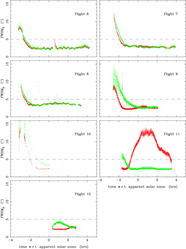
Figure 2: Limb edge width as a function of time (relative to apparent solar noon) throughout the seven successful SDS flights. The FWHM of the Gaussian fit to the derivative of the smoothed profile is shown for the direct image (red) and the reflected image (green) on the central CCD. The sparse data for Flight 10 is the result of an onboard recorder failure. The unusual behavior of the direct-image limb width during Flight 11 is also noteworthy. Solar diameter determinations are based only on those portions of each flight in which the FWHM of the direct and reflected images is relatively well-behaved. One such criterion is that the direct-image FWHM is below 5^′′, as shown by the dashed line. See Section 4.14 for a complete description of the data trimming criteria.

4 Data Analysis

An SDS flight typically consists of hundreds of thousands of individual exposures, each exposure imaging the Sun’s limb at ten different position angles, in total, across the seven CCDs (seen in Figure 1). The $7$-$\mu$sec duration exposures are grouped into “cycles” consisting of 18 exposures per cycle. The 18 exposures are completed within 0.22 sec and the time between successive cycles ranges from roughly 1 to 3 sec, depending on the flight. Pixel data from each cycle (7 CCDs times 18 exposures) are stored together in a single file, along with housekeeping data for the instrument at the time of observation. The post-flight processing pipeline treats a cycle’s worth of data at a time, although each exposure within a cycle is, for the most part, processed independently. Only in the final step (a correction based on the difference in width of opposite limbs of the Sun and its variation throughout the flight) does information from one cycle affect the analysis of another.

The sequence of steps in the processing pipeline is listed below and a detailed description of each step is given in the subsections that follow:

1. adjust photometrically, i.e., flatfield
2. remove “spike” artefacts
3. perform preliminary edge detection for all ten limbs
4. subtract background level and “ghost” image
5. make final edge determinations for the limbs using the cleaned profiles
6. correct for bias due to instrumental broadening of the limbs
7. transform CCD edge coordinates into focal-plane $(x,y)$
8. correct $(x,y)$ positions for optical distortion
9. correct $(x,y)$ positions for atmospheric refraction
10. fit direct and reflected image measures to two circular arcs
11. determine the minimum “gap” between direct and reflected limbs
12. calculate $R_{sun}$ in terms of the BSW angle
13. correct for Earth/Sun distance
14. detrend $R_{sun}$ as a function of delta limb width for the entire flight

4.1 Photometric adjustment

Prior to most flights, the response of the seven TC101 linear-array CCD detectors is calibrated from a series of benchtop observations of a reference sphere. A sequence of exposures of varying duration sample the full dynamic range of the detectors. From these measures, a quadratic function is fit to the CCD reading as a function of exposure time, on a per pixel basis. This is essentially a photometric bias plus nonlinear flatfield correction for each detector. Such calibration coefficients were determined prior to flights 6, 7, 8, 9 and 11. In some cases, all coefficients were determined in full (Flights 6 and 8) while in other cases only the constant (Flights 7 and 8) or constant and linear terms were redetermined (Flight 11) from the benchtop measurements.

In the data processing pipeline, each flight’s data are reduced using the corresponding pre-flight coefficient sets, with the exception of flights 10 and 11; the processing of these two flights makes use of the pre-flight 8 coefficients.

Subsequent to the application of these second-order coefficients, an additional photometric correction is needed. The TC101 detectors incorporate two amplifiers per detector, controlling separately the odd- and even-numbered pixels. The benchtop calibration sequences cannot account for differences in the bias levels between the two amplifiers as these change every time the electronics are powered. Thus, a scalar adjustment is calculated based on the empirical differences between neighboring even and odd pixel values, effectively putting all pixels on the photometric system of the odd pixels. The seven scalar corrections, one per detector, are calculated separately for each exposure within the flight. Figure 3 presents a sample profile of the central detector, before (red points) and after (blue points) the photometric adjustments are made. What appears to be two curves in the raw data is simply the result of the odd/even pixel offset.

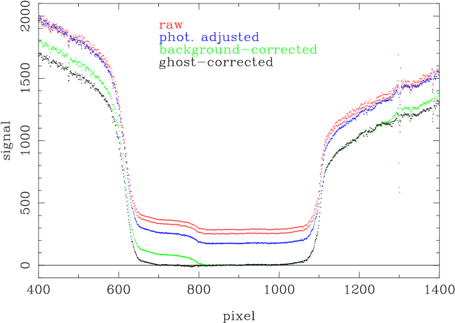
Figure 3: A sample SDS limb profile, obtained with the central CCD, at various stages of the reduction pipeline. The figure shows the raw profile (red); after photometric adjustment (blue); after background-level correction (green); and after the “ghost” image is subtracted (black). See the text for a description of the different correction steps.

4.2 Spike removal

Following the flatfield and bias corrections, the observed image profiles contain noise in the form of spikes that are one to several pixels wide and of relatively large amplitude. These spikes can fool the subsequent edge-detection algorithm, which relies on searching the numerical first derivative of the profile. For this reason, the profiles are filtered by examining the difference in value between each pixel and the average value of the pixels that fall 4 pixels to either side. Any pixel $i$ whose value differs by more than 120 counts has its value replaced by the $(i+4,i-4)$ pixels’ average. Note that the CCD gain is$\sim$8 e-/count and the 120-count spike threshold is 3 to 4 times the standard deviation of the signal for the portion of the CCDs containing the sun’s image. In practice, 0.1 % of the pixels are tagged as belonging to a spike. The spike-removal procedure effectively eliminates the problem of false edge detections.

4.3 Preliminary edge detection

We adopt as the conceptual limb edge the inflection point of the profile. This is determined by finding the maximum (or minimum, depending on whether the edge is a rising or falling one) in the first derivative of the profile. Unfortunately, the numerical derivative is noisy, creating local maxima and minima that confuse the edge detection routine. Thus, in practice, the profile is smoothed before differentiation. We use 20 repeated applications of a 3-pt smoothing. This necessary smoothing will unavoidably broaden the limb and, in doing so, will shift the inflection point. The shift, or bias, is a consequence of the difference in profile shape just before and after the inflection point. This bias will be corrected in a subsequent reduction step. Note that even absent the artificial smoothing introduced at this step in the reduction, other factors (primarily the instrument response) have already broadened the limb significantly. No matter the cause of the broadening, it will result in a bias in the measured inflection point position. The correction is calibrated as a function of the overall broadening and thus will correct for the overall bias, i.e., both the unavoidable component due to the instrument and that due to the 3-pt smoothing.

Once smoothed, a simple numerical derivative is obtained, $f^{\prime}_{i}=(f_{i+1}-f_{i-1})/2$. The index of the maximum value of $f^{\prime}_{i}$ is identified, and all adjacent points for which $f^{\prime}$ is greater than 0.5 times the maximum value are used to better refine the inflection point location. This refinement is by way of a Gaussian fit to the extracted points. The centre of the Gaussian is taken as the inflection point position. The FWHM of the best-fitting Gaussian is also stored. See Figure 4 for an illustration of the edge-fitting procedure. In this manner, preliminary positions for the ten limb edges are found, in terms of pixel position along the seven linear-array detectors.

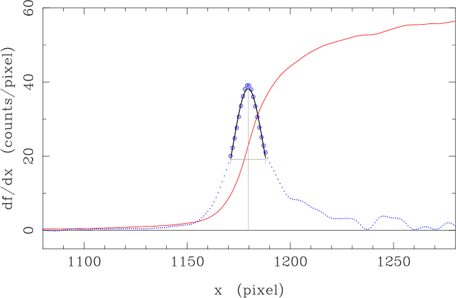
Figure 4: Illustration of the technique used to determine the inflection point position, $IPP$. The red curve is the smoothed limb profile. Shown in blue is the numerical first derivative of the profile. The heavy blue symbols indicate those points used in the least-squares Gaussian fit, which is shown by the black curve. The centre and FWHM of the fitted Gaussian are indicated by the gray line segments.

4.4 Background and ghost image subtraction

A careful examination of Figure 3 reveals the presence of a low-amplitude “ghost” of the main falling limb, lying in the valley between the falling (direct) and rising (reflected) limb images and offset from the main image by about 174 pixels. This image is due to a pair of internal reflections within a single element of the BSW. (The front and back surfaces of the two “flats” from which the BSW is composed are slightly non-parallel, to avoid fringing.) It is important to subtract this ghost image from the observed profile since its presence can affect the inflection point position, ($IPP$); primarily that of the falling limb because of the direction of the ghost-image offset. A ray-tracing model of the as-designed SDS optics predicts an offset of 178 pixels for the ghost image. Empirically, it is found to lie at an offset of 174 pixels. Its amplitude is a less predictable function of the coatings on the relevant surfaces of the BSW; coatings that deteriorate over time. For this reason, the relative amplitude of the ghost image is determined for each exposure, while the offset - which depends only on the assumed invariant geometry of the wedge - is set at 174 pixels.

Note that the rising-limb profile also has a contamination from its ghost, although it is difficult to detect as the direction of the offset causes it to fall entirely within the high-signal portion of that limb. Still, for the sake of consistency, this limb should also have the ghost profile removed.

In order to subtract the ghost-image profile properly, the relative amplitude of the direct and reflected limbs must be determined, as well as the relative amplitude of the ghost and main images. This is accomplished by measuring the amplitude of the central detector’s observed profile at key points with respect to the preliminary inflection point positions of the main limb edges, $IPP_{D}$ and $IPP_{R}$, as derived in the previous step.

The observed profiles in all of the SDS detectors are elevated by a background “sky” level that is a combination of true scattered light and uncorrected electronic bias, (presumably dominated by the latter). The background level is taken to be the minimum value of an 11-pixel-wide moving average within a conservatively limited range of pixels presumed to be free of either (direct or reflected) solar limb and their ghost images. The pixel ranges are based on the preliminary edge positions, the preliminary FWHM limb edge width, the 174-pixel ghost offset, and an additional cushion of 30 pixels. Thus, for detectors 6 and 7, which contain only the direct image limb on the low-pixel end of the detector, the signal-free pixel range is from the preliminary inflection point position $(IPP_{D})$ plus the FWHM plus the cushion up to 1728 minus the cushion. For detectors 1 and 5, which contain only the reflected image limb on the high-pixel end of the detector, the relevant range is from the cushion value up to the preliminary $IPP_{R}$ minus the FWHM minus the cushion. Finally, for detectors 2, 3 and 4, which contain both direct and reflected image limbs, the signal-free pixel range is from the preliminary $IPP_{D}$ plus the 174-pixel ghost offset plus the cushion and extending up to the preliminary $IPP_{R}$ minus the FWHM minus the cushion. Figure 3 shows a sample profile from detector #3 after subtraction of the background level calculated in this manner.

Having subtracted the background level, it is now possible to calculate the relative amplitudes of the various limb images - reflected relative to direct and ghost relative to main. This is accomplished by measuring the height of the profile in the central detector #3 at four key positions, i.e., just above the “knee” relative to the main direct and main reflected limb edges, and at similar pixel offsets relative to the projected positions of their respective ghosts. See Figure 5 for a schematic representation of these four key points. A simplified geometry for the underlying instrumental limb is shown for the sake of clarity, but the strategy is valid for the actual observed limb.

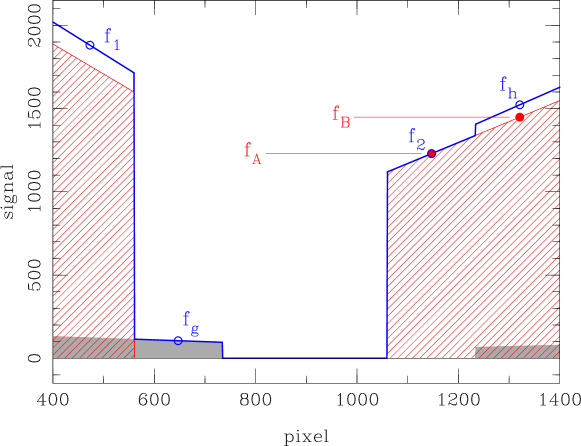
Figure 5: An idealized representation of the direct and reflected solar-limb profiles, as seen by the central detector, and their decomposition into “main-” and “ghost-”image contributions. The main images are shown in red-hatch shading; the direct-image limb to the left and the reflected-image limb to the right. Shaded in gray is the ghost image of the main image, which is caused by internal reflection within a single element of the beam splitting wedge. The ghost image is offset from the main image by 174 pixels and is greatly reduced in intensity. The main and ghost images combine to produce the observed total profile, represented by the heavy blue curve. By measuring the amplitude of the observed profile at key points relative to the direct- and reflected-limb edges (located at $\sim$560 and $\sim$1060, respectively, in the example shown), it is possible to deduce the relative intensity of the direct image to that of the reflected image, and the relative intensity of the ghost image to that of the main image.

The offset from the $IPP$ of a limb edge and what is meant by “just above the knee” is largely arbitrary; we take its value to be one half the ghost image offset, or $\Delta_{knee}$=87 pixels. Thus, the needed profile amplitudes are

$f_{1}\equiv f(x_{1})$ where $x_{1}=IPP_{D}-\Delta_{knee}$
$f_{g}\equiv f(x_{g})$ where $x_{g}=IPP_{D}+\Delta_{ghost}-\Delta_{knee}$
$f_{2}\equiv f(x_{2})$ where $x_{2}=IPP_{R}+\Delta_{knee}$
$f_{h}\equiv f(x_{h})$ where $x_{h}=IPP_{R}+\Delta_{ghost}+\Delta_{knee}$

Determination of the various $f_{i}$ is made by a linear fit to the observed profile at the pixel nearest $x_{i}$ along with its three neighbors on either side, and then evaluation of the fit at $x_{i}$. With $f_{1},f_{g},f_{2},$ and $f_{h}$ in hand, the relative amplitudes are derived in the following manner.

Assume the relative amplitude of the reflected and direct images is $\Gamma$, and the amplitude of the ghost profile relative to the main profile is $\gamma$. The observed, central-detector profile can be thought of as being built up from an intrinsic instrumental solar limb profile that has added to it a reflected, offset and scaled copy of itself, and then this combination having added to it a ghost copy of itself, with a separate offset and scaling factor. (In reality, there are second- and higher-order ghost images also present, but each of these is successively diminished by the factor $\gamma$ and in practice only the first-order ghost need be considered.)

For convenience, our formulation actually uses the main reflected image as the base template from which the overall profile is to be constructed. Adopting this, there are two points in the template profile that are useful to the formulation; call these $f_{A}$ and $f_{B}$, as shown in Figure 5. The four points measured in the observed profile can be written in terms of these two points’ amplitudes and the relative scale factors,

$$\begin{array}[]{l}f_{1}=f_{A}/\Gamma+\gamma f_{B}/\Gamma\\ f_{g}=\gamma f_{A}/\Gamma\\ f_{2}=f_{A}\\ f_{h}=f_{B}+\gamma f_{A}\end{array}$$ (1)

These can be combined to isolate the reflected-to-direct relative scale, $\Gamma$,

$$0=(f_{g}f_{g}/f_{2})\Gamma^{2}+(f_{1}-f_{g}f_{h}/f_{2})\Gamma-f_{2}.$$ (2)

Having found $\Gamma$, the ghost-to-main image relative scale, $\gamma$, can be determined,

$$\gamma=(f_{g}/f_{2})\Gamma.$$ (3)

Typical values of $\Gamma$ and $\gamma$ for the SDS flight data are approximately 0.7 and 0.06, respectively. These vary somewhat from flight to flight, as shown in Figure 6; presumably, this is due to aging of the surface coatings of the beam splitting wedge. This is discussed more thoroughly in Section 6.

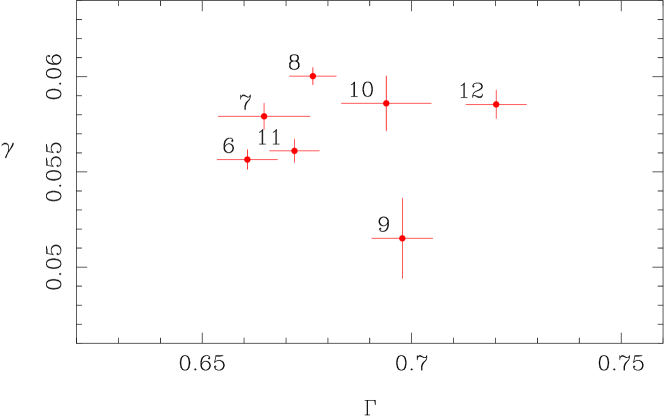
Figure 6: Ratio of the ghost-image amplitude to that of the main image ($\gamma$) versus the ratio of the reflected-image amplitude to that of the direct image ($\Gamma$). The data points are labelled by flight number. The “error” bars show the rms of the estimated ratios within each flight.

From the ghost scale factor, $\gamma$, and the assumed $\Delta_{ghost}=174$ pixel, it is possible to build a ghost-free template from the reflected-image portion of CCD#3’s profile. Our pipeline constructs one template per cycle from the average of the 18 exposures, interpolated and stored at a super-resolution of 0.1 pixels. Knowing the relative scale factors, ($\Gamma$ and $\gamma$), the preliminary main edge positions, ($IPP_{D}$ and $IPP_{R}$), and adopting a ghost-image offset of $\Delta_{ghost}=174$ pixels along CCD#3, the template can be used to subtract the ghost image from all the detectors’ profiles. Note that the ghost-image offset for the outer detectors, in pixels, is larger by a factor of $1/\cos(\theta)$, where $\theta=27.1^{\circ}$ is the angle between the outer detectors and the axis of deflection of the beam splitting wedge, which is approximately aligned with the inner detectors. Additionally, a pixel scale factor must also be applied to the template when used on the outer detectors to account for the slight misalignment of a radial for the main image and that of the ghost image. The misalignment is roughly $\phi=1.3^{\circ}$, and the correction factor is $\cos(\phi)$.

Using the above procedure, the ghost image can be subtracted from the observed profile in each of the seven detectors. The result for our sample CCD#3 profile is shown in Figure 3.

4.5 Final edge determination

With all pre-processing completed, including the subtraction of the ghost images, the inflection point positions ($IPP$s) are once again determined. This is done as before, using the Gaussian fit to the numerical first derivative procedure outlined in Section 4.3. The result is ten $IPP$s per exposure, along with accompanying FWHM measures.

4.6 Limb-broadening bias

The shape of the limb edge is asymmetrical about the inflection point. For this reason, any mechanism that broadens the limb will impart unequal amounts of influence from either side of the $IPP$ and, thus, will shift it. One expects (and finds) a one-to-one correspondence between limb width and the net amount of shift or bias. A calibration of this broadening bias can be made using a sufficiently accurate synthetic limb profile. The Code for Solar Irradiance (COSI, Haberreiter et al. 2008; Shapiro et al. 2010) calculates the solar spectral irradiance and has been used to calculate the intrinsic solar limb profile for the passband of the SDS. The profile provided by COSI was of sufficient resolution near the limb edge, but lacking toward the interior of the solar disk. For this reason, we have mated the COSI profile to the analytical solar limb prescription given by Hestroffer & Magnan (1998). The resulting synthetic profile is shown in Figure 7, scaled to nominal SDS pixels.

Applying the method of Section 4.3 (that of Gaussian fitting of the first derivative of the profile) provides the $IPP$ and FWHM for the intrinsic limb. The synthetic profile can then be broadened by a specified amount and the fitting procedure repeated, noting the shift in $IPP$ from that of the unbroadened profile. The $IPP$ shifts are plotted versus measured limb broadening in the inset panel of Figure 7. Two different forms of broadening were explored – multiple applications of simple three-point smoothing, and convolution with a Gaussian kernel. The resulting $IPP$-shift curve was practically identical for the two forms of broadening, being characterized only by the FWHM measure of the broadened limb. A best-fitting polynomial description of this calibration curve is incorporated into the SDS processing pipeline. The correction is calculated as the difference between the value of the calibration curve at FWHM=0.32 arcsec (the width of the unbroadened COSI profile) and its value at the measured FWHM of the limb edge being corrected. A FWHM-based bias correction is applied to the $IPP$ values of every limb-edge determination.

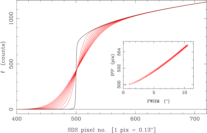
Figure 7: Calibration of the limb-broadening bias correction. The black curve displays the synthetic limb constructed from the COSI model mated to a Hestroffer & Magnan type profile, arbitrarily positioned at an SDS pixel value of 500. The red curves indicate the effect of successive smoothing (broadening) of the original profile. Using the method described in the text to determine the inflection point position ($IPP$), i.e., Gaussian fit to the profile’s first derivative, the shift in $IPP$ is a monotonic function of the limb width, as shown in the inset panel.

4.7 Transformation to Cartesian coordinates

The $IPP$s of the ten limb edges are each a one-dimensional measure of position along a linear-array CCD. These positions are transformed into focal-plane cartesian coordinates to facilitate circle-fitting of the direct and reflected disk images. The CCDs are soldered onto a ceramic mounting block, defining their orientations in the focal plane. The endpoints of the seven CCDs, i.e., the midlength points of the outer edges of the first and last active pixels, were measured in 1988 using the Yale PDS microdensitometer in opaque light-source mode. The repeatability of the endpoint measures was found to be $\sim 2$ microns. (The Yale PDS is a submicron-accuracy machine; difficulty in defining the low-contrast edges of the active areas of the SDS detectors was responsible for the 2-micron precision.)

Note that while 2 microns in the SDS focal plane corresponds to 20 mas, the geometric arrangement of the detectors - primarily the fact that the “gap” between direct and reflected image edges is measured within individual detectors - lessens the sensitivity of the derived solar radius to uncertainties in the detector positions. Monte-Carlo type tests in which the detectors were randomly offset and rotated by amounts consistent with the 2-micron uncertainty in their endpoint positions yielded just 3.5-mas variation (rms) in the resulting radius determinations. This amount, in quadrature, has little influence on what will be shown to be an overall 20-mas systematic error estimate for the SDS radius measures.

Concerned that numerous hard landings after balloon flights might have jarred the detector enough to shift the relative positions of the CCDs, the detector assembly was again measured in early 2012 using an OGP Avant 600 measuring machine also at Yale. The agreement between the 1988 PDS measures and the 2012 OGP ones is at an rms level of 4 microns, the expected accuracy of the OGP. Thus, it is reasonable to assume that the physical locations of the CCDs have remained stable over the course of the SDS balloon flights. The 1988 PDS endpoint measures are adopted for our analysis.

A simple linear interpolation of the $IPP$, in pixels, and the known $(x,y)$ positions of the CCDs’ endpoints provides the necessary transformation. Note that the detector assembly is typically unmounted and remounted between flights and an effort is made to align the central CCD with the wedge angle plane, such that the direction of offset of the reflected image coincides with CCD#3, the central detector. In practice, the alignment is not perfect and the circle-fitting procedure described in Section 4.10 allows us to determine the slight misalignment. The actual alignment is taken into consideration when determining the separation and minimum gap of the two fitted circles.

4.8 Optical distortion

Optical distortion of the as-designed SDS instrument has been determined independently using two different ray tracing programs. These agree in their finding that the maximum distortion occurs approximately 40 mm from the centre of the focal plane, with an amplitude of 0.018 mm. As discussed in the description of Step 10, the apparent radius of the direct disk image can differ from that of the reflected disk image, in general. One possible explanation for this asymmetry is an optical field-angle distortion (OFAD) that is not radially symmetric with respect to the centre of the detector plane. We have explored this possibility in two separate ways; by adopting the design OFAD but having it offset from the centre of the detector plane, and by using a ray tracing program to calculate the OFAD under the assumption that the Barlow lens is tilted by up to several degrees.

The first approach allows a reconciliation of the direct and reflected radii for Flights 6 through 8, given OFAD centre offsets of tens of mm. The ratio of radii is more deviant in Flights 9 through 12, ($R_{sunD}/R_{sunR}$=0.992); no amount of centre shift can bring the ratio to unity. However, the second approach, that of introducing a tilt in the Barlow lens, does allow the ratio to be forced to unity for all flights, using three different values of tilt, although the tilt angle exceeds $10^{\circ}$ for the later flights, an unrealistically large value. Still, it is informative that even under such extreme conditions of tilt and OFAD centre shifts, the effect on the resulting $R_{sun}$ values is slight.

A series of reductions of the SDS flight data have been made, using a large range of OFAD models and corrections. These sets of reductions are used to estimate the possible systematic errors in the final $R_{sun}$ values.

4.9 Atmospheric refraction

Even at the SDS float altitude (atmospheric pressure of 3 - 5 mbar), the instrument observes through some residual atmosphere and correction must be made for the effect of differential refraction over an angle corresponding to the size of the Sun. The formulation adopted is based on that of Smart (1979) and is described in detail by Sofia et al. (1994). In practice, the correction ranges from about 5 to 25 mas in the vertical direction and remains less than 5 mas in the horizontal direction.

4.10 Circle fitting

Having been corrected for distortion and refraction, the limb shape is taken to be circular; the solar oblateness being ignored at this point. The $IPP$s from a single exposure provide five points along the limb of the direct image and another five points along the limb of the reflected image. For each of the two disk images the points span an arc of about $54^{\circ}$, sufficient to define the circles. Each circle, uniquely specified by its radius and the $(x,y)$ location of its centre, is overdetermined by the five measures. The “geometric” best fitting circle to a set of points minimizes the sum of the squares of the distances of the points from the circle. This is a nonlinear least-squares problem, in general, but a numerically adequate and computationally fast approximate solution is available to us, given the particular layout of the SDS measures. The location of the two outer points, at roughly $\pm 27^{\circ}$ relative to the central concentration of three CCDs, naturally give the outer points a more prominent role in constraining the best-fitting circle. We adopt as an approximation to the geometric best-fit circle, the mean of the three distinct circles that are defined by the two outer points and each of the three inner points, in turn. This procedure assigns a slightly higher weight than deserved to the outer points, but, in practice, the random error introduced by this expedient approximation is negligible. In this manner, each SDS exposure yields radius and centre measures for both the direct and reflected disk images. The separation of the two centres determines the instantaneous pixel scale for the exposure. The two radii provide a helpful diagnostic and constraint on the form of the distortion correction, but these do not directly enter into the determination of $R_{sun}$. Instead, this derives from Equation 4 (in Section 4.12) and the measurement of the minimum gap between the two disk images.

4.11 Minimum gap determination

The minimum gap between the direct and reflected images is found from two separate quadratic functions describing $x$ as a function of $y$ for the three direct-image limb positions and the three reflected-image limb positions measured by the central CCDs. The gap is first measured in the coordinate system defined by CCD#3 and then corrected for the slight angle between this detector and the direction of displacement of the BSW, (as measured by the relative displacement of the direct and reflected disk image centres).

4.12 Calculation of $R_{sun}$

Referring to Figure 1, the angular half-diameter of the solar disk is

$$R_{sun}=W(1-d/D)$$ (4)

where $W$ is the wedge angle, nominally taken to be 989.47 arcsec, and $d$ and $D$ represent the gap and separation.

4.13 Correction for Earth/Sun distance

The SDS flights are made during northern-hemisphere fall, at which time the Earth/Sun distance is changing rapidly. It is a simple matter to correct the $R_{sun}$ measures within any flight to their corresponding values at 1 AU based on the well-known ephemeris of the Earth’s orbit. The distance at time of observation, in AU, functions as a simple scaling factor for the measured $R_{sun}$ values.

4.14 Dependence on direct/reflected limb-width difference

Despite the use of low-thermal expansion materials in the telescope assembly, the reliance on the stability of the BSW reference angle, and the correction of the $IPP$s for the in-flight variation of the measured limb widths, the resultant $R_{sun}$ measures tend to vary significantly throughout the cruise portions of the SDS flights. The cause of this variation is the differential behavior of the direct and reflected images throughout the flights, which is discussed further in Section 6. The SDS operating concept is based on the direct and reflected disk images differing only by their being offset by the BSW angle. And yet, the direct and reflected images’ observed properties do differ as witnessed by the measured widths of their respective limb images, (see Figure 2). Thus, a final, crucial correction must be made for the difference in the two image systems, one parametrized by the difference in limb widths. Figure 8 shows the strong correlation between measured $R_{sun}$ value and $\Delta$FWHM₃, the difference in measured FWHM of the direct and reflected limbs in the central CCD#3. The measures to be trusted are those in which the instrument performs as designed, with the direct and reflected images being similar in their properties, i.e., at $\Delta$FWHM${}_{3}=0$. In practice, instead of limiting ourselves to the relatively small number of exposures for which this holds absolutely true, we limit the exposures to those with $-2^{\prime\prime}<\Delta$FWHM${}_{3}<2^{\prime\prime}$ and adjust for the well-determined trends. Additionally, only data from each flight in which the central-CCD direct image FWHM $<$ 5 arcsec are used to calculate the solar diameter. This effectively discards from the analysis observations during the initial portion of each flight, prior to thermal equilibrium being reached, and the anomalous portion of Flight 11.

A suspected mechanism for the observed correlation with limb-width difference is asymmetry of the derivative profile, beyond that of the intrinsic solar limb profile. This has been explored, as detailed in Appendix A. While a portion of the in-flight variation can be explained as being due to instrument-induced skew in the derivative profiles, there is a significant portion of the variation that does not correlate with skew. Empirically, the measured diameter variation correlates best with $\Delta$FWHM and it is this correlation that we use to make the necessary correction.

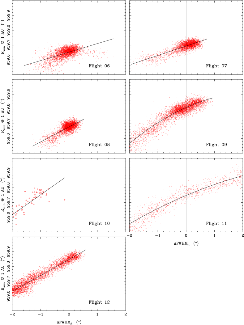
Figure 8: Measured solar half-diameter (corrected to 1 AU) as a function of difference in width of the direct- and reflected-image limb profiles on the central CCD detector. The linear or quadratic fits shown are applied to the flight data as a correction for the observed trend. Only data within the fitted range ($-2^{\prime\prime}<\Delta$FWHM $<2^{\prime\prime}$) are valid for correction; data outside this range are discarded. This results in the rejection of a large portion of Flight 11 data, as can be inferred from Figure 2.

Correcting for the trends seen in Figure 8 with a simple linear or quadratic fit (the results are largely insensitive to the form), the final measures of $R_{sun}$ throughout the seven flights are derived. Figure 9 shows the in-flight variation $R_{sun}$ prior to making the final $\Delta$FWHM correction. Figure 10 shows the post-correction values.

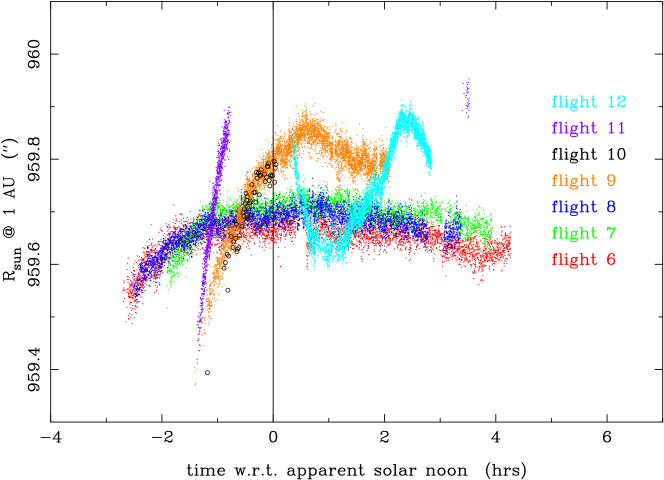
Figure 9: Solar half-diameter (corrected to 1 AU) as a function of time, relative to apparent noon, for the seven SDS flights presented here. The flights are color-coded as indicated in the legend. Only those portions of each flight that qualify for the determination of $R_{sun}$ are shown, i.e., direct-image FWHM $<5^{\prime\prime}$ and $-2^{\prime\prime}<\Delta$FWHM $<2^{\prime\prime}$. For the sake clarity, only one in every 25 such qualifying exposures is plotted, with the exception of Flight 10 for which all such exposures are shown.

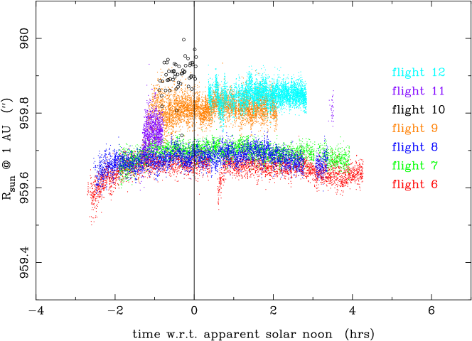
Figure 10: Same as Figure 9 but after having corrected for the dependence on limb-width difference, $\Delta$FWHM.

5 Solar-radius results

The final SDS measures of the solar half-diameter, after making all necessary corrections and adjustments described in the previous section, are listed in Table  3. Dates of observation are expressed in fractional years and the half-diameter measures are given in arcsec. The uncertainties listed are $1\sigma$ estimates of the combined random and time-dependent systematic errors. In all cases but one, (that one being Flight 10), the systematic component is dominant. We estimate the systematic uncertainties from the variation of $R_{sun}$ values resulting from limiting cases of assumptions related to the corrections listed in Section 4, primarily the treatment of optical distortion. That is, reductions were made in which the assumed optical distortion was as designed and with perfect alignment, as well as with distortion fields assumed to be offcentre and/or with a Barlow-lens misalignment chosen to force the ratio of direct- and reflected-image radii to unity. The standard deviation of the $R_{sun}$ value differences was 20 mas and we adopt this as the systematic component of the uncertainties. In the case of Flight 10, the small number of recoverable exposures taken at float altitude resulted in a formal random uncertainty of up to 20 mas, depending on specifics of the data trimming. We have chosen, conservatively, to add the random and systematic error contributions for Flight 11 directly, instead of in quadrature, resulting in a total estimated uncertainty of 40 mas for this measure. The majority of the data from Flight 11 also had to be discarded because of the anomalous behavior of the limb-width during much of the flight, but even with these data removed, the formal random error was insignificant relative to the estimated 20-mas systematic component. To be specific, the formal random error for Flight 10 is 20 mas; for Flight 11, it is 0.3 mas; and for the remaining flights it is less than 0.1 mas. The systematic component of the total uncertainties listed in Table 3 is assumed to be the same for each flight and is estimated to be 20 mas.

Table 3: SDS Solar-radius results

Flt.	Epoch	$R_{sun}@$ 1 AU $(^{\prime\prime})$
6	1992.82	959.638 $\pm$ 0.020
7	1994.81	959.675 $\pm$ 0.020
8	1995.82	959.681 $\pm$ 0.020
9	1996.85	959.818 $\pm$ 0.020
10	2001.83	959.882 $\pm$ 0.040
11	2009.87	959.750 $\pm$ 0.020
12	2011.86	959.856 $\pm$ 0.020

Note that the present results supersede all previous analyses and presentations of SDS solar-diameter measures. Those previous studies included only a portion of the components of the present analysis; most importantly, they lacked the final adjustment based on the difference between direct- and reflected-image limb widths. Another difference of the current analysis is that besides addressing the known optical processes that affect the results, we have explicitly considered the uncertainties corresponding to our treatment such processes.

6 Discussion

The $R_{sun}$ values from Table 3 are plotted in the top panel of Figure 11. Based on the estimated precision and stability of the SDS, a significant variation of the photospheric solar radius with time is apparent. Are there alternative explanations for the measured variation, apart from an intrinsic change in the Sun’s size?

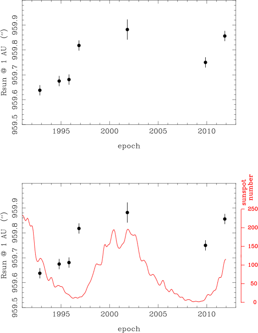
Figure 11: Final values of the SDS-measured solar half-diameter (corrected to 1 AU) as a function of time. The error bars indicate $1\sigma$ estimates of the combined random and systematic uncertainties. For comparison, in the lower panel, the SDS results are plotted along with NOAA-tabulated monthly sunspot numbers for the same period.

The most obvious explanation is that the SDS internal calibration is failing, in some way, from flight to flight. As we have emphasized, the stability of the wedge – critically, that of the angle between the second and third surfaces responsible for the reflected image – is the basis of our astrometric calibration. SDS construction uses fused silica and Zerodur optical components and structural supports made of Invar to minimize thermally induced flexure during its Sun-pointed observing runs. Still, as indicated by the variations in the limb-edge widths shown in Figure 2, the SDS optical properties are seen to vary throughout each flight, particularly so during the last four flights. To the extent that the direct and reflected image paths vary in unison, the width-bias correction and pixel-scale adjustment of Section 4 compensate for the expected effect on the limb edge positions, provided the limb-width excursions are not overwhelming. For this reason we discard frames in which the FWHM of the direct image on the central detector exceeds 5 arcsec.

More troubling are the portions of flights in which the direct and reflected image properties vary substantially from one another, the bulk of Flight 11 being the most egregious example of this behavior, (see Figure 2). A temperature-sensitive ray tracing model of the SDS was explored in an attempt to understand how the reflected-image limb width might maintain nominal behavior while the direct-image limb width performed such a wild excursion. (The inverse behavior would be more readily understood, as a perturbation associated with the two extra reflections experienced by the reflected beam.) We found that the mid-Flight-11 widths could be modeled by a specific combination of thermal gradients in the first element of the BSW; a 1$-^{\circ}$C radial gradient (edge to center), and a 5$-^{\circ}$C axial gradient (front to back surface). The former induces a negative power in the first BSW element, affecting both the direct and reflected images. This is a result of both a physical deformation of the fused silica element (coefficient of thermal expansion, $\alpha_{TE}=5.2\times 10^{-7}/^{\circ}$C) and of the temperature dependence of its index of refraction ($dn/dT=1.0\times 10^{-5}/^{\circ}$C). The axial gradient, via thermal expansion, also induces a shape change of the reflecting back surface of the first BSW element, which, if “tuned,” can cancel the refractive effect of the radial gradient and bring the reflected beam back into focus while the direct beam remains out of focus. Yet, this explanation also predicts that the effective focal lengths of the direct and reflected channels would differ by 11% while in this state. Such a large scale difference would be readily seen in the ratio of derived disc radii for the direct and reflected images and nothing anywhere near this level is observed. Also, while these balancing thermal gradients could account for the mid-flight widths, it is highly improbable that the onset and eventual dissipation of the gradients, as evidenced by the normal width behavior at the start and end of the flight, would maintain such a tricky balance, i.e., the reflected-image width behavior never deviates far from that seen in other flights. Thus, we feel this model does not, specifically, explain the extreme behavior during the middle of Flight 11. However, qualitatively, thermally induced shape and/or refractive perturbations of the BSW from its equilibrium configuration are a likely explanation for the observed differences in the limb-width behavior of the direct and reflected images throughout each flight. If so, one would expect a deviation from the BSW’s equilibrium shape to produce a deviation in the resulting solar diameter measure. For small perturbations, the correlation should be linear, exactly as we find empirically in the limb-width difference adjustment of Section 4.14 and Figure 8. The critical issue, as far using the BSW as a calibration for SDS, is if its equilibrium shape varies from flight to flight.

The high-altitude environment and thermal load associated with pointing at the Sun should be relatively consistent for the SDS, from flight to flight. On the other hand, one can expect a slow deterioration of the reflective coatings on the BSW surfaces with time, thus, possibly affecting the instrument’s in-flight equilibrium state under similar thermal stress. The deterioration of a subset of the surface coatings can be monitored by examining the relative heights of the reflected and direct solar images, $\Gamma$, from Equation 2. Using the same portions of each flight that were used to determine the mean solar diameter estimates, i.e., filtering by direct-image width and difference in reflected and direct image widths on the central detector, we list the mean relative heights in Table 4. The rms variation of $\Gamma$ within each flight is typically $\sim$0.01. Overall, there is a gradual trend with time; a slightly larger fraction of light makes it into the reflected image. To see if this results in a detectable flight-to-flight change in the equilibrium shape of the wedge, we examine the offset of the ghost image limb edge from that of the main image, (see Figure 5 and the discussion in Section 4.4). Recall that the ghost image is due to an extra internal reflection within an element of the BSW; the front and back surfaces were purposefully made non-parallel to avoid fringing. Again restricting ourselves to the useful portion of each flight, the mean values of $\Delta_{ghost}$ are included in Table 4. The values are in arcseconds, having been adjusted using simultaneous measures of the pixel scale based on the separation of the solar disc centres. The rms within each flight is roughly 0.2 arcsec. To the extent that a radial thermal gradient changes the shape of the front BSW element, the ghost image offset should vary by a proportional amount. In fact, the mean ghost offset is remarkably stable over the final five flights. What variation is observed, does not correlate with the variation in the measured solar half-diameter values. We repeat the mean half-diameter estimates in the table for comparison.

Table 4: BSW diagnostics by flight

Flt.	Epoch	$\Gamma$	$\Delta_{ghost}(^{\prime\prime})$	$R_{sun}(^{\prime\prime})$
6	1992.82	0.661	22.80	959.638
7	1994.81	0.665	23.15	959.675
8	1995.82	0.676	22.97	959.681
9	1996.85	0.698	22.97	959.818
10	2001.83	0.692	23.02	959.882
11	2009.87	0.672	22.97	959.750
12	2011.86	0.720	22.97	959.856

From this, we find no direct evidence that the BSW geometry, and thus the SDS calibration angle, is changing from flight to flight. On the other hand, the underlying cause of the variation in the direct- and reflected-image limb widths throughout each flight remains not fully understood. A comprehensive structural/thermal/optical analysis might shed further light, but at this point resources for an accurate modelling of the as-built SDS are not available. Such an model could not be relied upon to make quantitative, “open-loop” corrections to the instrument scale and distortion, for instance, but it might provide a theoretical basis for the empirical adjustments that we employ in our reduction procedure.

In the above analysis, $\Gamma$ is sensitive to changes in the reflection/transmission properties of the coatings on the second and third BSW surfaces while $\gamma$ is associated with internal reflections from potentially both BSW elements. All four surface coatings combine to define the passband, roughly 100 nm wide and centred around 600 nm. It is conceivable that with a deterioration of the surface coatings the passband could change. Judging from its roughly constant signal level, the throughput of the instrument has not changed drastically over the seven flights, although this has not been measured precisely. Considering the relatively wide passband of the SDS, the effective depth of the Sun’s atmosphere being observed will not be strongly wavelength dependent. Thus, it is unlikely that evolution of the instrument’s passband is responsible for the observed half-diameter changes. Besides, one would expect deterioration to yield a monotonic change in the passband while the observed half diameter is seen to fluctuate.

Even if the BSW-based calibration of the SDS is reliable, there is another possible explanation for the apparent variation in the solar diameter worth addressing. The variation might be caused by measurement error associated with solar surface activity, should a surface feature at the Sun’s limb fall on one or more of the SDS detectors. Of course, the frequency and density of such features will fluctuate throughout the solar cycle, possibly giving rise to a false diameter change signature. This explanation is disproved by the fact that the diameter variations are not in-phase with the activity cycle, as shown by the lower panel in Figure 11. Here the measured half-diameter values are plotted alongside a tracing of the NOAA-tabulated sunspot counts over the same period.

Additionally, the SDS is stepped through rotations during each flight, such that the diameter measures are made at different solar latitudes. Measurements at all latitudes are included here, thus lessening any possible dependence on low-latitude activity. (It is in the determination of oblateness, the subject of a future study, that an effect due to activity is likely to be seen, if at all.) By averaging the SDS measures over large fractions of each flight, the mean radius over a range of solar latitude is actually what is determined. For most of the SDS flights the effective mean solar colatitude measured, $\overline{\theta_{l}}$, is extremely consistent. The exceptions to this are Flight 10 (loss of most data due to a recorder failure), Flight 11 (rejection of anomalous limb profile data), and Flight 12 (restricted rotation sampling due to reduced telescope control). The expected flight-to-flight variation in measured radius due to this effect, assuming an elliptical limb shape, is $\delta cos(2\overline{\theta_{l}})$, where $\delta$ is the actual difference in equatorial and polar radius. In Flights 6 through 9 the geometric factor, $cos(2\overline{\theta_{l}})$, is less than 0.1. Assuming a nominal solar oblateness of 8 mas would induce a systematic variation from flight to flight that is negligible. Even in Flights 10 through 12, the factor is at most 0.4, leading to a maximum systematic offset of 3 mas from the uneven sampling in solar latitude. This is still insignificant relative to the estimated 20 mas systematic uncertainty of each flight’s radius determination. No discernible variation in measured radius as a function of SDS telescope rotation angle (or in solar latitude observed) is seen beyond the expected $\sim$10 mas variation associated with true oblateness. Thus, we conclude that neither solar activity or solar oblateness – nor, more directly, instrument observing angle – can account for the flight-to-flight diameter variation observed.

In summary, we find it reasonable to conclude that what the SDS has detected are real changes (both increases and decreases) of the solar radius. These are too small to be confirmed by ground-based telescopes, and too few to ascertain its time behavior. Our results contrast with the only alternative space-borne radius values published to date (Kuhn et al. 2004), which indicate no radius changes over nearly two decades. However, they were obtained with the MDI experiment on SOHO, which does not have on-board calibration.

We note that f modes of the Sun can also be used to find a measure of the solar radius. Frequencies of solar f modes bear a very simple relationship to stellar structure. They are most sensitive to the total mass and radius of the Sun and not to the details of solar structure. Solar models constructed with the conventional value of the solar radius usually have f-mode frequencies that do not match the Sun. This gave rise to the concept of the “seismic” radius of the Sun (Schou et al. 1997, Antia, 1998). The seismic radius basically defines where the kinetic energy of the modes is the maximum. The seismic radius of the Sun appears to be somewhat smaller than the photospheric radius. More interestingly, helioseismic data show that the Sun’s seismic radius varies with changes in solar activity (Antia et al. 2000); in the sense that the seismic radius decreases with increase in solar activity. By comparison, the photospheric radius variations (i.e., those presented here, as determined from limb position) are much larger and not in phase with the activity cycle. This can be understood by the fact that the radius variations are not homologous (Sofia et al. 2005; Lefebvre et al. 2007), with different mass shells expanding by different amounts.

Simultaneous measurements of the photospheric and seismic radii are of great interest since they will allow us to calibrate solar models better. Differences and similarities of the temporal behavior of these radii should contain information on how and where magnetic fields linked to activity change solar structure (Sofia & Li 2001, Li et al. 2003).

7 Conclusions

Accurate, long-term measurement of the diameter of the Sun is an admittedly difficult undertaking, fraught with issues of instrument stability and calibration. The SDS design overcomes these challenges by relying on a beam splitting wedge, constructed using optical contact bonding, to provide side-by-side images of the Sun separated by a stable reference angle. The dual images transform the relatively large angular measure into a small displacement in the instrument’s focal plane, and also provide a number of diagnostic parameters that can be used to monitor and internally calibrate the diameter measurements throughout each SDS flight. The SDS data-analysis procedure, presented here in detail, allows direct comparison of results over the decades-long program.

The balloon-borne SDS experiment has measured the angular size of the Sun seven times over the period 1992 to 2011. The half-diameter is found to change over that time by up to 200 mas, whereas the estimated uncertainties of the measures, random plus systematic, are typically 20 mas. The variation is not in phase with the solar activity. Thus, the measured variation is not an artefact of observational contamination by surface activity. While the SDS measures span 19 years, they are sparse, making it impossible to say with any certainty that the observed variation is cyclic.

The temporal behavior of the Sun’s photospheric radius provides a key constraint on models of solar structure, particularly with regard to the location, geometry, and evolution of subsurface magnetic fields. Because radius variations might have significant implications regarding the effects of solar variability on climate change (Sofia & Li 2001), it is necessary to make further efforts to confirm or refute the changes reported in this paper, to further refine its magnitude, and to establish its time behavior. This requires a long series of observations which are well calibrated and made from space, or a space-like environment.

An experiment that has spanned nearly three decades is only possible with the support and collaboration of many people and institutions. Beyond the co-authors of this paper, we would first like to thank the people who assisted in its conception and design; this includes E. Maier, K. Schatten, P. Minott, H-Y. Chiu, and A. Endal. The fabrication of the SDS payload could not have been accomplished without D. Silbert. Flight operations were helped by many people including D. Pesnell, and W. Hoegy. We are, of course, grateful for the substantial financial support provided by a series of grants from NASA and the NSF, and more recently, from the G. Unger Vetlesen Foundation, and the Brinson Foundation. CNES (France) and CNRS (France), which support the PICARD/SODISM mission, also provided financial support for the most recent SDS flight and we thank these institutes for their contribution. Understanding of the SDS instrument response was greatly assisted by the COSI model provided by A. Shapiro and optical modelling by L. Ramos-Izquierdo as well as modelling and other contributions by W. van Altena, R. Mendez and D. Casetti. Our work benefited from previous versions of the SDS analysis pipeline constructed by J. Zhang, A. Egidi, B. Caccin, and D. Djafer. Also, insightful comments from an anonymous referee led to significant improvements in the manuscript. Finally, we want to acknowledge the outstanding flight support provided by the personnel of the NASA/Columbia Scientific Balloon Facility over the years.

Appendix A Profile skew and $IPP$ shift

As discussed in Section 4.6, broadening of the limb edge profile by a symmetric kernel function results in a shift of the $IPP$ because of an asymmetry in the underlying, intrinsic limb profile. This shift is characterized by the measured FWHM as shown in Figure 7. Additional $IPP$ shift or bias will be incurred if the broadening mechanism itself imparts an asymmetry, i.e., if the instrument point spread function is asymmetric.

Such asymmetry, beyond that expected from the intrinsic limb profile, is seen in the SDS observations when the FWHM rises above its nominal 2 to 3 arcsec value. Figure 12 illustrates this for an exposure during Flight 12. Numerical derivatives of the smoothed limbs, measured on the central detector, are shown for a case where the direct and reflected images yield FWHM values of 2.1 and 4.1 arcsec, respectively. There is significant skew in the broader, reflected-image profile. The local inflection point differs from the Gaussian-fit center ($x$=0 in the figure) by 2 to 3 pixels, while the expected shift using the calibration curve of Figure 7 is only 1 pixel. The instrument (in this case, its reflected-image channel) must be responsible for the additional asymmetry.

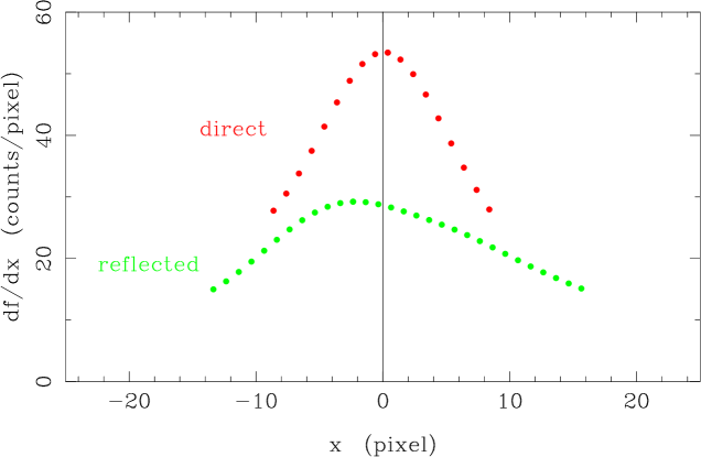
Figure 12: Sample limb-edge profile pair in which the reflected-image limb shows skew while the direct-image limb does not. The numerical derivative of the smoothed profile is from a single exposure on the central detector, midway through Flight 12. $x$=0 corresponds to the Gaussian-fit center for each limb, while the FWHM is 2.1 and 4.1 for the direct and reflected images, respectively.

A better fit to such a profile can be made by employing an asymmetric fitting function. Alternatively, a symmetric fitting function can still be used provided the range of data points to be included in the fit is sufficiently limited. Recall that the portion of the profile to be fit was somewhat arbitrarily chosen to be those data points contiguous to the maximum point and with values greater than half the maximum. As a test, we choose the second approach, adopting the quadratic defined by the maximum point in each profile and its neighboring two points. While the use of just three points per profile will make for noisy $IPP$ determinations, it is systematic effects we wish to explore here.

We apply this $IPP$-determination method to Flights 07 and 12, and plot the resulting half-diameters in Figure 13, (red points). For comparison, we also plot the half diameters resulting from the standard (Gaussian fit) pipeline, before (black points) and after (blue points) the final $\Delta$FWHM correction of Section 4.14. An artificial offset of +/-0.3 arcec has been added to separate the three sets for clarity.

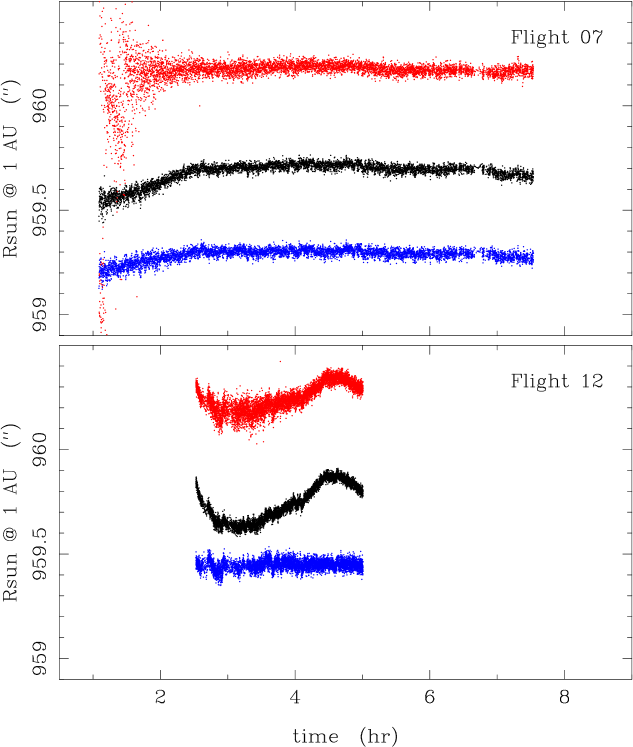
Figure 13: Comparison of $IPP$-fitting methods for Flight 07 (upper panel) and Flight 12 (lower panel). Solar half diameter, corrected to 1 AU, is shown as a function of the raw in-flight time, which has an arbitrary zero point. In each panel, the central (black) points show the $R_{sun}$ measures based on the standard pipeline but before the final $\Delta$FWHM correction, while the lower (blue) points show the same data after the $\Delta$FWHM correction. Using the alternative, three-point quadratic-fit $IPP$ method results in the half diameter measures shown by the upper (red) set of points. The latter sets of points are artificially displaced by +/-0.3 arcsec for the sake of clarity.

Assuming the Sun’s true angular diameter is constant throughout each flight, it appears the three-point quadratic $IPP$ method does an equally good job of flattening the flight curve as does the $\Delta$FWHM-correction method. In fact, in terms of systematics, if not random noise, it is superior during the initial ascent phase of the flight. Although, during this stage the FWHM value exceeds 5 arcsec and, thus, the standard pipeline would have rejected these data for the purpose of diameter determination.

For Flight 12, the conclusion is different; the three-point quadratic $IPP$ method does not yield a constant half diameter while the standard pipeline, with the $\Delta$FWHM correction, does. Note that during Flight 07 the direct and reflected limb widths track one another well, while during Flight 12 they do not, (see Figure 8).

References

- (1)
- (2) Antia, H. M. 1998, A&A 330, 336
- (3)
- (4) Antia, H. M., Basu, S., Pintar, J., Pohl, B. 2000, SoPh 192, 459
- (5)
- (6) Assus, P., Irbah, A., Bourget, P., Corbard, T., & the PICARD Team 2008, Astron. Nach. 329, 517
- (7)
- (8) Brown, T. M. & Christensen-Dalsgaard, J. 1998, ApJ 500, 195
- (9)
- (10) Bush, R. I., Emilio, M., Kuhn, J. R. 2010, ApJ 716, 1381
- (11)
- (12) Delmas, C. & Laclare, F. 2002, SoPh 209, 391
- (13)
- (14) Djafer, D., Thuillier, G., Sofia, S. 2008, ApJ 676, 651
- (15)
- (16) Egidi, A., Caccin, B., Sofia, S., Heaps, W., Hoegy, W., Twigg, L. 2006 SoPh 235, 407
- (17)
- (18) Fivian, M. D., Hudson, H. S., Lin, R. P., Zahid, H. J. 2008, Science 322, 560
- (19)
- (20) Fivian, M., Hudson, H. S., Lin, R. P., Bush, R. I., Emilio, M., Kuhn, J. R., Scholl, I. F. 2012, AAS Meeting #220, #205.11
- (21)
- (22) Haberreiter, M., Schmutz, W., Kosovichev, A. G. 2008, ApJ 675, 53
- (23)
- (24) Hestroffer, D. and Magnan, C. 1998, A&A 333, 338
- (25)
- (26) Kuhn,J. R., Bush, R. I., Emilio, M., Scherrer, P. H. 2004, ApJ 613, 1241
- (27)
- (28) Lefebvre, S., Kosovichev, A. G., Rozelot, J. P. 2007, ApJ 658, 135
- (29)
- (30) Li, L. H., Basu, S., Sofia, S., Robinson, F. J., Demarque, P., Guenther, D. B. 2003, ApJ 591, 1267
- (31)
- (32) Noël, F. 2004, A&A 413, 725
- (33)
- (34) Pap, J., Rozelot, J. P., Godier, S., Varadi, F. 2001, A&A 372, 1005
- (35)
- (36) Penna, J. L., Jilinski, E. G., Andrei, A. H., Puliaev, S. P., Reis Neto, E. 2002, A&A 384, 650
- (37)
- (38) Schou, J., Kosovichev, A. G., Goode, P. R., Dziembowski, W. A. 1997, ApJ 489, 197
- (39)
- (40) Shapiro, A. I., Schmutz, W., Schoell, M., Haberreiter, M., Rozanov, E. 2010, A&A 517, 48
- (41)
- (42) Smart, W. M. 1979, “Spherical Astronomy” (6th ed.; New York, Cambridge University Press), p 72
- (43)
- (44) Sofia, S., Maier, E., Twigg, L. W. 1991, Adv. Space Res. Vol 11, No. 4, 123
- (45)
- (46) Sofia, S., Heaps, W., Twigg, L. W. 1994, ApJ 427, 1048
- (47)
- (48) Sofia, S. & Li, L. H. 2001, J. Geophys. Res. 106, 12969
- (49)
- (50) Sofia, S., Basu, S., Demarque, P., Li, L., Thuillier, G. 2005, ApJ 632, 147
- (51)
- (52) Thuillier, G., Dewitte, S., Schmutz, W., & the PICARD Team 2006, Adv. Space Res. Vol 38, No. 8, 1792
- (53)
- (54) Thuillier, G., Sofia, S., Haberreiter, M. 2005, Adv. Space Res. Vol 35, No. 3, 329
- (55)
- (56) Thuillier, G., Dewitte, S., Schmutz, W., & the PICARD Team 2011, in IAGA Special Sopron Book Series, Vol. 4: “The Sun, the Solar Wind, and the Heliosphere”, Proc. of the conf. held 23-30 August, 2009 in Sopron, Hungary, eds. M. P. Miralles and J. Sánchez Almeida, (Berlin: Springer), p 365
- (57)
- (58) Wittmann, A. D. 2003, Astron. Nachr. 324 No. 4, p 378
- (59)