redMaPPer I: Algorithm and SDSS DR8 Catalog

Abstract

We describe redMaPPer, a new red-sequence cluster finder specifically designed to make optimal use of ongoing and near-future large photometric surveys. The algorithm has multiple attractive features: (1) It can iteratively self-train the red-sequence model based on a minimal spectroscopic training sample, an important feature for high redshift surveys; (2) It can handle complex masks with varying depth; (3) It produces cluster-appropriate random points to enable large-scale structure studies; (4) All clusters are assigned a full redshift probability distribution $P(z)$; (5) Similarly, clusters can have multiple candidate central galaxies, each with corresponding centering probabilities; (6) The algorithm is parallel and numerically efficient: it can run a Dark Energy Survey-like catalog in $\sim$ 500 CPU hours; (7) The algorithm exhibits excellent photometric redshift performance, the richness estimates are tightly correlated with external mass proxies, and the completeness and purity of the corresponding catalogs is superb. We apply the redMaPPer algorithm to $\sim 10,000\,\mathrm{deg}^{2}$ of SDSS DR8 data, and present the resulting catalog of $\sim$ 25,000 clusters over the redshift range $z\in[0.08,0.55]$. The redMaPPer photometric redshifts are nearly Gaussian, with a scatter $\sigma_{z}\approx 0.006$ at $z\approx 0.1$, increasing to $\sigma_{z}\approx 0.02$ at $z\approx 0.5$ due to increased photometric noise near the survey limit. The median value for $|\Delta z|/(1+z)$ for the full sample is $0.006$. The incidence of projection effects is low ($\leq 5\%$). Detailed performance comparisons of the redMaPPer DR8 cluster catalog to X-ray and SZ catalogs are presented in a companion paper.

1. Introduction

Over the past several years, galaxy clusters have been recognized as powerful cosmological probes (e.g., Henry et al. 2009; Vikhlinin et al. 2009; Mantz et al. 2010; Rozo et al. 2010; Clerc et al. 2012; Benson et al. 2013; Hasselfield et al. 2013). Galaxy clusters are one of the key probes of Dark Energy for ongoing and upcoming photometric surveys such as the Dark Energy Survey (DES: The DES Collaboration 2005), Pan-STARRS (Kaiser et al. 2002), the Hyper-Suprime Camera (HSC), and the Large Synoptic Survey Telescope (LSST: LSST Dark Energy Science Collaboration 2012).

Because galaxies are obviously clustered on the sky, rich galaxy clusters have been detected as far back as the 1800’s (Biviano 2000), with the first large catalogs generated from galaxy overdensities on photographic plates created 50 years ago (e.g., Abell 1958; Zwicky et al. 1968; Abell et al. 1989). More recently, the advent of multi-band data has led to a proliferation of optical cluster finding algorithms. These algorithms use various techniques for measuring clustering in angular position plus color/redshift space, ranging from simple matched-filters to more complicated Voronoi tesselations. These cluster finders can be divided into roughly two classes, those based on photometric redshifts (e.g., Kepner et al. 1999; van Breukelen & Clewley 2009; Milkeraitis et al. 2010; Durret et al. 2011; Szabo et al. 2011; Soares-Santos et al. 2011; Wen et al. 2012), and those utilizing the cluster red-sequence (e.g., Annis et al. 1999; Gladders & Yee 2000; Koester et al. 2007a; Gladders et al. 2007; Gal et al. 2009; Thanjavur et al. 2009; Hao et al. 2010; Murphy et al. 2012). However, relatively few of these optical catalogs have been utilized for cosmological parameter constraints (e.g., Rozo et al. 2007, 2010; Mana et al. 2013).

Given the above landscape, it is a fair question to ask whether the world really needs yet another photometric cluster finding algorithm. As we describe below, we believe that the answer to this question is yes. In particular, there are a variety of important features that any reasonable optical cluster finder must have in order to properly exploit the photometric data that will become available with ongoing or near-future photometric surveys such as the DES or LSST.

What must we require of current photometric cluster finders? The key features are as follows.

1. The algorithm must be able to smoothly detect galaxy clusters in a consistent way across a braod redshift range. This can be a challenge for photometric redshift (“photo-$z$”) and red-sequence based algorithms alike. For photometric redshift based algorithms, one must be cautious because biases and scatter in reported photo-$z$s increase at fainter magnitudes where spectroscopic training and validation samples can be highly incomplete. For red-sequence based cluster finders, one must confront the fact that the $4000\,\mathrm{\AA}$ break characteristic of the early-type galaxy spectra moves across filters. While $g-r$ is an ideal color for cluster detection at low redshift, one should rely primarily on $r-i$ at itermediate redshifts, and $i-z$ at higher redshifts (and we note that this will also affect photo-$z$-based finders). By $z\approx 1$, near-infrared (NIR) photometry is required. Being able to smoothly transition from one color to the next — or better yet, to always use all available photometric data — is paramount.

2. To the extent possible, the algorithm should self-train to the available data. For instance, algorithms reliant on a priori parameterizations of the red sequence could easily result in systematic biases if the a priori parameterization differs from reality. Note that this also impacts photo-$z$-based cluster finders, since there can be unknown and difficult to calibrate biases in the photometric redshifts of cluster galaxies.

3. The algorithm should be numerically efficient, capable of running on extremely arge data sets within reasonable timeframes with modest computational resources.

4. The algorithm must be able to properly account for complex survey masks, including varying depth.

5. The algorithm must allow the construction of proper cluster-random points that adequately characterize the effective survey volume for cluster detection in order to enable large scale structure studies. In particular, it is worth emphasizing that because galaxy clusters are extended objects on the sky, the galaxy mask used to construct the cluster catalog is not the appropriate mask characterizing the angular and redshift selection of galaxy clusters for any particular cluster finder.

6. The algorithm should produce a full $P(z)$ distribution for every cluster. Similarly, given that the center of a galaxy cluster can be observationally uncertain, there should be a corresponding centering distribution in the plane of the sky $P(\bm{\hat{n}})$. Note that if one adopts the prior that a galaxy resides at the center of a galaxy cluster, then the probability $P(\bm{\hat{n}})$ collapses to the probability that any given cluster galaxy is the correct cluster center. Our expectation is that just as $P(z)$ allows one to adequately recover the redshift distribution of galaxy clusters in a statistical sense, so too will centering probabilities for cluster galaxies allow one to statistically recover the angular distribution of clusters in the sky, a point that is of critical importance for large-scale structure studies.

7. In order to maximize the cosmological utility of the derived cluster samples, the richness estimators should be fully optimized for the purpose of minimizing the scatter in the richness–mass relation.

The red-sequence Matched-filter Probabilistic Percolation (redMaPPer) cluster finding algorithm is our solution to the above list of must-haves. Concerning the last point in particular, over the past several years we have empirically explored what works and what does not work in estimating cluster richness (Rozo et al. 2009, 2011; Rykoff et al. 2012, henceforth R12). For instance, we have demonstrated that estimating membership probabilities for every galaxy is very effective, while using hard color cuts to derive cluster membership can lead to large biases. We have fully optimized the optical detection radii, as well as the luminosity cuts employed when counting galaxies. We have also investigated whether total galaxy counts or total cluster luminosity is a better mass proxy, and whether or not trying to add blue galaxies into richness estimates results in improvements. All of these lessons have gone into the creation of the redMaPPer cluster finder.

There, is however, one feature of redMaPPer that represents more of a personal bias as opposed to an empirically driven choice, namely, the fact that redMaPPer is a red-sequence cluster finder. Indeed, operationally, redMaPPer can be easily adapted to work in photo-$z$-space rather than working directly in color-space. However, we are wary of reliance on photometric redshifts, which become increasingly difficult to characterize for faint galaxies due to a lack of spectroscopic training and validation samples. Furthermore, cluster galaxies are a very particular population, and photo-$z$ estimates tailored for clusters should be derived separately from the total galaxy population. Though there have been some studies comparing different cluster finders (e.g., Goto et al. 2002; Bahcall et al. 2003; Lopes et al. 2004, Paper II), we have not seen any conclusive evidence for photo-$z$-based algorithms outperforming red-sequence methods or vice-versa. Here, we have opted to rely on a red-sequence method when developing redMaPPer. Of course, at high enough redshift, as the red-sequence begins to disappear, it is obvious that photometric redshift methods must necessarily perform better (e.g., Eisenhardt et al. 2008; Brodwin et al. 2011). We do not, however, expect this to be a problem for near-future large photometric surveys. Note that while it is true that redMaPPer also relies on spectroscopic training samples, an important advantage of our novel red-sequence modeling alogirhtm is that we do not require a locally representative training sample: our spectroscopic training galaxies can be the brightest cluster galaxies at all redshifts, with no degradation in the performance of our photometric redshift estimates.

The redMaPPer algorithm is designed to handle an arbitrary photometric galaxy catalog, with an arbitrary number of photometric bands ($\geq 3$), and will perform well provided the photometric bands span the $4000\,\mathrm{\AA}$ break over the redshift range of interest. It is thus well suited to current surveys such as the Sloan Digital Sky Survey (SDSS: York et al. 2000) for low and moderate redshift clusters ($z\in[0.05,0.55]$), as well as upcoming surveys such as DES for low and high redshift clusters ($z<1$). As a case study, in this paper we present the redMaPPer catalog as run on $10,400\,\mathrm{deg}^{2}$ of photometric data from the Eighth Data Release (DR8: Aihara et al. 2011) of the SDSS. We will make the full DR8 redMaPPer catalog available after this paper is accepted for publication.

The layout of this paper is as follows. In Section 2, we describe the SDSS data used for this work, followed in Section 3 with an overall outline of the redMaPPer cluster finder. In Section 4 we describe the multi-color richness estimator $\lambda$, which is an update of the single-color richness estimator used in R12. In Section 5 we describe our strategy for dealing with stellar masks and regions of limited depth in the survey. In Section 6, we describe the self-training of the red sequence parametrization used to detect clusters, as well as measure their photometric redshifts, which is described in Section 7. In Section 8 we describe our new probabilistic cluster centering algorithm. Finally, in Section 9 we put all these pieces together into the redMaPPer cluster finder. The resulting SDSS DR8 redMaPPer cluster catalog is described in Section 10. Next, in Section 11, we describe a new, more accurate method of using the survey data to estimate the purity and completeness of the cluster catalog, and in Section 12 we describe how these methods can be applied to generate a cluster detection mask over the full sky. A summary is presented in Section 13. In the appendices we present several systematic checks, including Appendix B which contains an estimate of the minimum number of training spectra required for an accurate red-sequence calibration. A full detailed comparison of redMaPPer and other large photometric survey catalogs to X-ray cluster catalogs is presented in a companion paper (Paper II: Rozo & Rykoff 2014). When necessary, distances are estimated assuming a flat $\Lambda$CDM model with $\Omega_{m}=0.27$, and $h=1.0\ \mbox{Mpc}$, i.e., all quoted distances are in $h^{-1}\,\mathrm{Mpc}$.

2. Data

As discussed above, the redMaPPer algorithm is designed to handle an arbitrary photometric galaxy catalog, with an arbitrary number of photometric bands ($\geq 3$). Of course, the quality of the output depends on the quality of the photometry. As a case study, in this paper we run redMaPPer on SDSS DR8 data, due to its large area and uniform coverage.

2.1. SDSS DR8 Photometry

The input galaxy catalog for this work is derived from SDSS DR8 data (Aihara et al. 2011). This data release includes more than $14,000\,\mathrm{deg}^{2}$ of drift-scan imaging in the Northern and Southern Galactic caps. The survey edge used is the same as that used for Baryon Acoustic Oscillation Survey (BOSS) target selection (Dawson et al. 2013), which reduces the total area to $\approx 10,500\ \deg^{2}$ with high-quality observations and a well-defined contiguous footprint. Similarly, bad field and bright star masks are based on those used for BOSS.

The BOSS bright star mask is based on the Tycho catalog (Høg et al. 2000). However, this catalog is incomplete at the bright end. Cross-matching Tycho to the Yale Bright Star Catalog (Hoffleit & Jaschek 1991), covering 9000 of the brightest stars in the sky (mostly visible to the naked eye), we have found an extra 70 stars — including very bright stars such as Arcturus and Regulus — that obviously impacted galaxy photometry and detection. We have also found that very large, bright galaxies such as M33 cause significant problems for photometry in the area, including many spurious sources marked as galaxies. To handle these issues, we have visually inspected and masked obviously bad regions around 63 objects brighter than $V<10$ from the New General Catalogue (NGC: Sinnott 1988) that are in the DR8 footprint, as well as the bright stars mentioned above. In total, an additional $36\,\mathrm{deg}^{2}$ ($\sim 0.3\%$ of the total area) is removed by our combined bright star and galaxy mask. After accounting for all the masked regions, the input galaxy catalog covers $10,400\,\mathrm{deg}^{2}$.

As discussed in R12, the careful selection of a clean input galaxy catalog is required for proper cluster finding and richness estimation. Our input catalog cuts are similar to those from Sheldon et al. (2012) used for BOSS target selection, with some modifications. First, we select galaxies as classified by the default SDSS star/galaxy separator. We further limit our catalog to $i<21.0$, approximately the $10\sigma$ limiting magnitude for the survey. We then filter all objects with any of the following flags set in the $g$, $r$, or $i$ bands: SATUR_CENTER, BRIGHT, TOO_MANY_PEAKS, and (NOT BLENDED OR NODEBLEND). Unlike the BOSS target selection, we have chosen to keep objects flagged with SATURATED, NOTCHECKED, and PEAKCENTER.

Particular care has to be made in avoiding over-aggressive flag cuts because of the way that the SDSS photo pipeline handles dense regions such as cluster cores. In these cases, the central galaxy and many satellites may be originally blended into one object and then deblended. However, if there is a problem with one part of the parent object — such as a cosmic ray hit that is not properly interpolated — then this bad flag is propagated to all the children. We have found that removing objects marked with SATURATED, NOTCHECKED, and PEAKCENTER often mask out cluster centers, while truly saturated objects such as improperly classified stars are also rejected via the SATUR_CENTER flag cut. Overall, by including these objects we increase the number of galaxies in the input catalog by less than $2\%$, and our tests have shown no significant effect on the richness measurements except for a few clusters for which the cores were inadvertently masked out when galaxies with the above flags were removed. In total, there are 56.5 million galaxies in the input catalog.

In this work, we use CMODEL_MAG as our total magnitude in the $i$ band, and MODEL_MAG for $u$, $g$, $r$, $i$, and $z$ when computing colors. We limit our input catalog to galaxies that have $m_{i}<21.0$, approximately the $10\sigma$ limit for galaxy detection such that the characteristic magnitude error for our faintest objects is $\sim 0.1$. The DR8 übercalibration procedure yields magnitude uniformity on the order of 1% in $griz$ and 2% in $u$. The resulting color scatter introduced by the photometry is significantly narrower than the width of the cluster red sequence. All magnitudes and colors are corrected for Galactic extinction using the dust maps and reddening law of Schlegel et al. (SFD: 1998).

2.2. Spectroscopic Catalog

Although our cluster finder uses only photometric data, we require spectroscopic data to calibrate the red sequence and to validate our photometric redshifts. For this purpose we use the SDSS DR9 spectroscopic catalog (Ahn et al. 2012). This spectroscopic catalog has over 1.3 million galaxy spectra, including over 500,000 Luminous Red Galaxies (LRGs) at $z\sim 0.5$ from the CMASS sample. As detailed below, we only use $\approx 20\%$ of the available data in our training, and use the remaining data set to validate our photometric redshifts.

3. Outline of the Cluster Finder

The redMaPPer algorithm finds optical clusters via the red sequence technique. More specifically, it is built around the optimized richness estimator $\lambda$ developed in R09 and R12. The algorithm is divided into two stages: a calibration stage, where we empirically calibrate the properties of the red sequence as a function of redshift; and a cluster-finding stage, where we utilize our calibrated model to identify galaxy clusters and measure their richness. The algorithm is iterative. First, an initial rough color calibration is used to identify clusters. These clusters are then used to better calibrate the red sequence, which enables a new cluster finding run (see also Blackburne & Kochanek 2012, for a similar approach within the context of cluster finding with spectroscopic data sets). These two calibration/cluster finding stages are iterated several times before a final cluster finding run is made.

The calibration itself is also an iterative procedure described in detail in Section 6. We start with a set of “training clusters” that have a red central galaxy with a spectroscopic redshift to calibrate the red sequence model. As we show in Appendix B, our minimal training requirements for unbiased cluster richness and photometric redshift estimation are $\approx 40$ clusters per redshift bin of width $\pm 0.025$. In the case of SDSS DR8, the spectroscopic availability greatly surpasses this requirement by many orders of magnitude. However, for upcoming surveys such as DES probing much higher redshifts, this will no longer be the case, and we have developed redMaPPer with these limitations in mind.

For the present work on DR8, we construct our sample of training clusters from red spectroscopic galaxies. These red galaxies are used as “seeds” to look for significant overdensities of galaxies of the same color. The significant overdensities thus become our training clusters that are used to fit a full linear red-sequence model (including zero-point, tilt, and scatter) to the sample of all high-probability cluster members with a luminosity $L\geq 0.2L_{*}$. This luminosity threshold is optimal for richness measurements (R12). In this way we effectively transfer the “seed” spectroscopic redshift to all high probability cluster members, which enables a much more accurate measurement of the red sequence. This is especially true for fainter magnitudes where there is very limited spectroscopic coverage. Note that because the algorithm utilizes all colors simultaneously, the “scatter” is characterized not by a single number but by a covariance matrix.

Given a red-sequence model, the cluster finding proceeds as follows (see Section 9 for details). First, we consider all photometric galaxies as candidate cluster centers (thereby assuming the center of a cluster is located at a galaxy position). We use our red-sequence model to calculate a photometric redshift for each galaxy ($z_{\mathrm{red}}$; see Section 7.1), and evaluate the goodness of fit of our red galaxy template. Galaxies that are not a reasonable fit to the red galaxy template at any redshift are not considered as possible central galaxies for the purpose of cluster ranking. We note that as long as a cluster has at least one galaxy that is a reasonable fit to the template, that cluster will be considered in the first step of the cluster-finding stage. We then use the $z_{\mathrm{red}}$ value of the candidate central galaxy as an initial guess for the cluster redshift. Based on this redshift, we compute the cluster richness $\lambda$ and its corresponding likelihood using a multi-color generalization of the method of R12 (see Section 4). When a significant number of red-sequence galaxies ($\geq 3$) is detected within a $500\,h^{-1}\,\mathrm{kpc}$ aperture, we re-estimate the cluster redshift by performing a simultaneous fit of all the high probability cluster members to the red sequence model. This procedure is iterated until convergence is achieved between member selection and cluster photometric redshift ($z_{\lambda}$; see Section 7.2). The resulting list of candidate cluster centers is then rank-ordered according to likelihood. Starting with the highest ranked cluster we measure the richness and membership probabilities. These probabilities are then used to mask out member galaxies for lower-ranked clusters in a process we term “percolation” (see Section 9.3). In this way we prevent double-counting of galaxy clusters.

4. Richness Estimator $\lambda$

The redMaPPer richness estimator, $\lambda$, is a multi-color extension of the richness estimator developed in R09 and R12, which we now denote $\lambda_{\mathrm{col}}$ to indicate that it is a single-color richness. Here we review how we calculate $\lambda$ and highlight the differences relative to R12.

Let $\bm{x}$ be a vector describing the observable properties of a galaxy (e.g., multiple galaxy colors, $i$-band magnitude, and position). We model the projected distribution within and around clusters as a sum $S(\bm{x})=\lambda u(\bm{x}|\lambda)+b(\bm{x})$ where $\lambda$ is the number of cluster galaxies, $u(\bm{x}|\lambda)$ is the density profile of the cluster normalized to unity, and $b(\bm{x})$ is the density of background (i.e., non-member) galaxies. The probability that a galaxy found near a cluster is actually a cluster member is simply

$$p_{\mathrm{mem}}=p(\bm{x})=\frac{\lambda u(\bm{x}|\lambda)}{\lambda u(\bm{x}|\lambda)+b(\bm{x})}.$$ (1)

We note that in Section 9.3, the definition of the membership probability will be modified to allow for proper percolation of the cluster finder. This modification will only impact clusters that are close to each other along the line of sight and at comparable redshifts. Regardless, the total number of cluster galaxies $\lambda$ must satisfy the constraint equation

$$\lambda=\sum p(\bm{x}|\lambda)=\sum_{R<R_{c}(\lambda)}\frac{\lambda u(\bm{x}|\lambda)}{\lambda u(\bm{x}|\lambda)+b(\bm{x})}.$$ (2)

The corresponding statistical uncertainty in $\lambda$ is given by

$$\mbox{Var}(\lambda)=\sum p(\bm{x}|\lambda)\left[1-p(\bm{x}|\lambda)\right].$$ (3)

In principle, these sums should extend over all galaxies. In practice, one needs to define a cutoff radius $R_{c}$ and a luminosity cut $L_{\mathrm{cut}}$. In R12 and Rozo et al. (2011) we showed that the scatter in the mass–richness relation is expected to be minimized when $L_{\mathrm{cut}}=0.2L_{*}$, while the optical radial cut scales with richness via

$$R_{c}(\lambda)=R_{0}(\lambda/100.0)^{\beta}.$$ (4)

where $R_{0}=1.0\,h^{-1}\,\mathrm{Mpc}$ and $\beta=0.2$. We adopt these parameters in redMaPPer.

To determine the cluster richness of a galaxy cluster, note that $\lambda$ is the only unknown in Eqns. 2 and 4. Therefore, we can numerically solve Eqn. 2 for $\lambda$ using a zero-finding algorithm. The solution to Eqn. 2 defines $\lambda$, and naturally produces a cluster radius estimate $R_{c}$ via Eqn. 4. We emphasize this cluster radius is not a proxy for any sort of standard overdensity radius such as $R_{500c}$ or $R_{200m}$.

As in R12, we consider three observable properties of galaxies for our filter function $u(\bm{x})$: $R$, the projected distance from the cluster center; $m_{i}$, the galaxy $i$-band magnitude, and a color variable. Ideally, our color variable would be the full color vector (e.g., $\mathbf{c}=\{u-g,g-r,r-i,i-z\}$ in the case of SDSS data). However, practical considerations forced us to reduce this information to a single $\chi^{2}$ value which gives the goodness of fit of our red-sequence template. In doing so, we effectively compress the information contained in the multi-dimensional color vector into a single number that measures the “distance” in color space between the galaxy of interest and our red sequence model. This is described in more detail below.

We adopt a separable filter function

$$u(\bm{x})=[2\pi R\Sigma(R)]\phi(m_{i})\rho_{\nu}(\chi^{2}),$$ (5)

where $\Sigma(R)$ is the two dimensional cluster galaxy density profile, $\phi(m)$ is the cluster luminosity function (expressed in apparent magnitudes), and $\rho_{\nu}(\chi^{2})$ is the $\chi^{2}$ distribution with $\nu$ degrees of freedom. The pre-factor $2\pi R$ in front of $\Sigma(R)$ accounts for the fact that given $\Sigma(R)$, the radial probability density distribution is $2\pi R\Sigma(R)$. We summarize below the filters used in redMaPPer.

4.1. The $\chi^{2}$ Filter

Assume we have a multicolor red sequence model for which we have $\left<\mathbf{c}|z,m_{i}\right>$, the mean color of the red sequence galaxies for any given redshift $z$ and $i$-band magnitude $m_{i}$. Furthermore, assume we have a corresponding covariance matrix $\mathbf{C}_{\mathrm{int}}(z)$ to describe the intrinsic scatter and correlations of galaxy colors about the mean.

When comparing a given galaxy with color vector $\mathbf{c}$ to the model color, with the assumption of Gaussian errors the distribution of galaxies will be represented by a $\chi^{2}$ distribution:

$$\chi^{2}(z)=\left(\mathbf{c}-\left<\mathbf{c}|z,m_{i}\right>\right)\left(\mathbf{C}_{\mathrm{int}}(z)+\mathbf{C}_{\mathrm{err}}\right)^{-1}\left(\mathbf{c}-\left<\mathbf{c}|z,m_{i}\right>\right)$$ (6)

where $\mathbf{c}$ is the color vector of the galaxy under consideration, $m_{i}$ is the observed galaxy magnitude, $\left<\mathbf{c}|z,m_{i}\right>$ is the model color, and $\mathbf{C}_{\mathrm{int}}(z)$ is the corresponding covariance matrix, which itself depends on redshift. The matrix $\mathbf{C}_{\mathrm{err}}$ describes the photometric error of the galaxy under consideration.

For red sequence cluster members, $\chi^{2}$ will be distributed according to the $\chi^{2}$ distribution with $\nu$ degrees of freedom,

$$\rho_{\nu}(\chi^{2})=\frac{(\chi^{2})^{(\nu/2-1)}e^{-\chi^{2}/2}}{2^{\nu/2}\Gamma(\nu/2)},$$ (7)

where $\nu$ is the number of colors employed when estimating $\chi^{2}$. Note that for $\nu=1$ the $\chi^{2}$ filter does not reduce to the single color filter of R12. This is because our distance measurement $\chi^{2}$ does not distinguish between galaxies that are too red from galaxies that are too blue, so there is some loss of information when moving from color-space to $\chi^{2}$. While a full $\nu$-dimensional Gaussian color filter would work better than our $\chi^{2}$ filter — and would exactly reduce to the single color $\lambda_{\mathrm{col}}$ from R12 when $\nu=1$ — the problem of background estimation for such a filter is much more difficult. In particular, in the case of DR8, it requires one to estimate the galaxy density in a five dimensional space: $\{m_{i},u-g,g-r,r-i,i-z\}$. We found these background estimates to be very noisy, so we compressed the color information to a single variable $\chi^{2}$. In this way, at any given redshift the background depends only on $m_{i}$ and $\chi^{2}$.

4.2. The Radial and Luminosity Filters

For the radial filter, we follow R09 and R12 and adopt a projected NFW profile (Navarro et al. 1995), which is a good description of the dark matter profile in N-body simulations. In addition, it has been found to be a good description of the radial distribution of cluster galaxies (Lin & Mohr 2004; Hansen et al. 2005; Popesso et al. 2007). In R12 it was shown that in order to minimize the scatter in the mass–richness relation the NFW filter works as well or better than other possible radial profiles. Therefore, we refer readers to Section 3.1 of R12 for details on the form of the radial filter.

For the luminosity filter, we similarly follow R09 and R12 and adopt a Schechter function (e.g., Hansen et al. 2009), written as

$$\phi(m_{i})\propto 10^{-0.4(m_{i}-m_{*})(\alpha+1)}\exp\left(-10^{-0.4(m_{i}-m_{*})}\right).$$ (8)

In an update from R12, we have set $\alpha=1.0$ independent of redshift, which provides a better description of the data. The characteristic magnitude, $m_{*}$, is the same as used in R12, calculated for a k-corrected passively evolving stellar population (Koester et al. 2007b). In the redshift range $0.05<z<0.7$, appropriate for DR8, $m_{*}(z)$ is well approximated ($\delta<0.02\,\mathrm{mag}$) by the following polynomials:

$$m_{*}(z)=\begin{cases}22.44+3.36\ln(z)+0.273\ln(z)^{2}&\text{if $z\leq 0.5$,}\\ \,\,-0.0618\ln(z)^{3}-0.0227\ln(z)^{4}&\\ 22.94+3.08\ln(z)-11.22\ln(z)^{2}&\text{if $z>0.5$.}\\ \,\,-27.11\ln(z)^{3}-18.02\ln(z)^{4}\end{cases}$$

For each cluster, $m_{*}$ is taken at the appropriate redshift and the luminosity filter is normalized to unity at the appropriate magnitude cutoff. As with R12, this is taken to be $0.2L_{*}$, or $m_{*}+1.75\,\mathrm{mag}$. Although in the current version of redMaPPer both $\alpha$ and $m_{*}$ are fixed as described above, in future releases we will replace these parameters with those directly measured from calibration clusters. We emphasize, however, that modest changes to the shape of the luminosity filter result in insignificant changes to the recovered richness. Of course, changes to the magnitude limit above which one counts galaxies has an obvious systematic impact on the richness as one moves up and down the luminosity function, although we have found these modest shifts no not signifcantly impact the mass–richness scatter (see R12).

4.3. Background Estimation

As in R12, we assume that the background density is uniform, such that $b(\bm{x}|z)=2\pi R\bar{\Sigma}_{g}(m_{i},\chi^{2}|z)$ where $\bar{\Sigma}_{g}(m_{i},\chi^{2}|z)$ is the galaxy density as a function of galaxy $i$-band magnitude and $\chi^{2}$, where $\chi^{2}$ is evaluated using the red sequence model at redshift $z$. In this way, the effective background for every cluster is different and depends on the cluster redshift. Note that since clusters reside in overdense regions, this mean background is likely an underestimate of the true background, but the incurred bias is small (see R12 and Rozo et al. 2011), and is irrelevant for cosmological purposes, as it is completely degenerate with the amplitude of the richness–mass relation. Variability of the background (which is expected) is more problematic, and can lead to catastrophic projections. These are expected to be small (Rozo et al. 2011), and will be addressed in a future paper (Rozo et al., in preparation).

To calculate the mean galaxy density, we first calculate the $\chi^{2}$ value for all galaxies in a grid of redshifts with spacing 0.02. For computation purposes, we only calculate the $\chi^{2}$ for galaxies that are brighter than $0.1L_{*}$ at a given redshift bin. This implies that the magnitude range being sampled is different for each redshift bin. At each redshift we bin the full galaxy catalog in $\chi^{2}$ and magnitude using a cloud-in-cells (CIC) algorithm (e.g., Hockney & Eastwood 1981), and divide by the survey area. For our cells, we use $\chi^{2}\in[0,20]$ with a bin size of 0.5, and $i\in[12,m_{\mathrm{lim}}]$ with a bin size of 0.2. The $\chi^{2}<20$ cut can be justified by the fact that the sum total of cluster membership probability in the redMaPPer catalog for galaxies with $\chi^{2}\in[15,20]$ is only $0.7\%$. That is, our $\chi^{2}<20$ cut impacts our results at well below the $1\%$ level. The final galaxy number density is normalized by the width of each color and magnitude bin. To evaluate the background at an arbitrary redshift, we linearly interpolate between the backgrounds computed along our redshift grid. As noted in R12, because the background is measured per square degree, the average number of background galaxies as a function of $\chi^{2}$, magnitude, and redshift is automatically accounted for as the angular size of the clusters changes with redshift.

5. Handling Masked Regions and Limited Depth

In an ideal world, our survey would have uniform depth, be deep enough to reach $0.2L_{*}$ at all redshifts of interest, and there would be no missing and/or masked regions, e.g., due to bright stars. Most previous optical cluster finders make this simple assumption. Here, we describe how we can properly correct for these effects. Our approach is conceptually straightforward. Given a cluster model and a geometric and magnitude mask, we can effectively calculate the fraction of cluster galaxies that we expect to be masked out. This correction factor is then applied to the “raw” richness to compensate for the masked region. In practice, this correction can be self-consistently incorporated into the richness estimation, as described below. Our method is simple to implement with any geometric mask, including those that describe variations in depth. However, we do not take into account masks that contain one or more missing bands.

5.1. The Correction Term

Looking back at Eqn. 2, we have:

$$1=\sum_{i}\frac{u(\bm{x}_{i})}{\lambda u(\bm{x}_{i})+b(\bm{x}_{i})},$$ (9)

where $\bm{x}_{i}$ describes the radial position, color (via $\chi^{2}$), and luminosity (via $m_{i}$) of each galaxy. This formulation works if we can see all galaxies, but in reality we cannot. Let us then pixelize all observable space $\bm{x}$ into infinitesimal pixels, and let $N_{i}$ be the number of galaxies in pixel $i$. Most pixels have $N_{i}=0$, but a few have $N_{i}=1$. Thus, the sum over all galaxies can be re-written in terms of a sum over all pixels via:

$$1=\sum_{i}N_{i}\frac{u(\bm{x}_{i})}{\lambda u(\bm{x}_{i})+b(\bm{x}_{i})}.$$ (10)

In the case of masking, we can only observe the galaxies that are inside the mask, so we can split this sum into:

$$1=\sum_{\mathrm{in}}N_{i}\frac{u(\bm{x}_{i})}{\lambda u(\bm{x}_{i})+b(\bm{x}_{i})}+\sum_{\mathrm{out}}N_{i}\frac{u(\bm{x}_{i})}{\lambda u(\bm{x}_{i})+b(\bm{x}_{i})}.$$ (11)

The “in” term is the raw $\lambda$ that we usually compute, and can be replaced by the standard sum over all observed galaxies. The “out” term is now a correction to the standard expression, call it $C$,

$$C=\sum_{\mathrm{out}}N_{i}\frac{u(\bm{x}_{i})}{\lambda u(\bm{x}_{i})+b(\bm{x}_{i})}.$$ (12)

In terms of $C$, Eqn. 2 can be rewritten as

$$1-C=\sum_{\mathrm{gals}}\frac{u(\bm{x})}{\lambda u(\bm{x})+b(\bm{x})}.$$ (13)

Now, while $C$ is unknown (we cannot see the masked region), we can compute its expected value for a cluster of richness $\lambda$. Using the fact that

$$\left<N_{i}\right>=[\lambda u(\bm{x}_{i})+b(\bm{x}_{i})]\Delta\bm{x}_{i},$$ (14)

we see that the expectation value of $C$ is given by

$$\left<C|\lambda\right>=\int_{\mathrm{out}}d\bm{x}\ u(\bm{x}).$$ (15)

In the above equation, we have made explicit the fact that $C$ depends on $\lambda$, both via the cutoff radius used in the sum over galaxies, and because the radial filter depends on $\lambda$. Thus, in the presence of missing data, our richness estimate is given by the solution to

$$1-\left\langle C|\lambda\right\rangle=\sum_{\mathrm{gals}}\frac{u(\bm{x})}{\lambda u(\bm{x})+b(\bm{x})}.$$ (16)

Note, however, that because $C$ is a unknown, there must also be additional measurement error associated with this unknown correction. To calculate the variance of $C$, we note that $\mathrm{Var}(N_{i})=\left<N_{i}\right>$. To compute $\mathrm{Cov}(N_{i},N_{j})=\left<N_{i}N_{j}\right>-\left<N_{i}\right>\left<N_{j}\right>$, we first compute $\left<N_{i}N_{j}\right>$. For infinitesimal pixels, $N_{i}N_{j}=1$ implies that either both pixels $i$ and $j$ contain cluster galaxies, or that one pixel contains a cluster galaxy while the other pixel contains a background galaxy, or that both pixels contain a background galaxy. Consequently,

$$P(N_{i}N_{j}=1)=\Delta\bm{x}^{2}[\lambda(\lambda-1)u_{i}u_{j}+\lambda(u_{i}b_{j}+u_{j}b_{i})+b_{i}b_{j}].$$ (17)

Since $\left<N_{i}N_{j}\right>=P(N_{i}N_{j}=1)$, subtracting off $\left<N_{i}\right>\left<N_{j}\right>$ we arrive at

$$\mathrm{Cov}(N_{i},N_{j})=-\Delta\bm{x}^{2}u_{i}u_{j}$$ (18)

for $i\neq j$. Putting it all together, we arrive at

$$\mathrm{Var}(C) = \sum_{i}\left\langle N_{i}\right\rangle p_{i}-\sum_{i}\sum_{j\neq i}\mathrm{Cov}(N_{i},N_{j})p_{i}p_{j}$$ (19)

$$= \int_{\mathrm{out}}d\bm{x}\ u(\bm{x})p(\bm{x})-\left[\int_{\mathrm{out}}d\bm{x}\ u(\bm{x})p(\bm{x})\right]^{2}.$$ (20)

To propagate the error in $C$ into the error in $\lambda$, we set

$$\sigma_{\lambda}=\frac{d\lambda}{dC}\bigg{|}_{\lambda(\left<C\right>)}\sigma_{C},$$ (21)

where $\sigma_{C}=[\mathrm{Var}(C)]^{1/2}$. The derivative of $\lambda$ with respect to $C$ is evaluated numerically about the expectation value of $\left\langle C|\lambda\right\rangle$, where $\lambda$ is the solution to Eqn. 16.

For future reference, it will be useful to define the “scale factor”

$$S(z)=\frac{1}{1-\left\langle C|z\right\rangle}$$ (22)

for the case in which the only source of masking is due to limited depth. With this definition, a cluster with richness $\lambda$ has a total of $\lambda/S(z)$ galaxies above the limiting magnitude of the survey.

In addition, it is useful to calculate the fraction of the effective cluster area that is masked solely by geometrical factors such as bright stars, bad fields, and survey edges. This is complementary to $S(z)$ defined above in that it contains all the masking except the magnitude limit. The cluster mask fraction is then

$$f_{\mathrm{mask}}=\frac{\int_{\mathrm{out}}dx\ u(x)}{\int dx\ u(x)}.$$ (23)

This quantity is very useful because clusters that are strongly affected by edges are more likely to be catastrophically miscentered, and to have poor richness estimates. Consequently, when defining our cluster catalog we will apply a cut in $f_{\mathrm{mask}}$.

5.2. Evaluating the Mask Correction

Evaluation of the mask correction and its associated error on $\lambda$ can be difficult. Fortunately, this problem is well suited to Monte Carlo integration. First, define the selection function ${\cal S}(\bm{x})$, so that ${\cal S}(\bm{x})=1$ if the galaxy is in a region where it is detected, and ${\cal S}(\bm{x})=0$ if the position $\bm{x}$ is masked out. Then, for any function $f(x)$,

$$\int_{\mathrm{out}}d\bm{x}\ f(\bm{x})=\int_{\mathrm{cluster}}[1-{\cal S}(\bm{x})]f(\bm{x})d\bm{x},$$ (24)

where the integral on the right hand side is over the full cluster region, i.e., $R\in[0,R(\lambda)]$, $L\geq L_{\mathrm{min}}$, and over all colors.

Applying this to Eqn. 15 we find

$$\left<C\right>=\int_{\mathrm{cluster}}[1-{\cal S}(\bm{x})]u(\bm{x})d\bm{x}.$$ (25)

Since $u(\bm{x})$ is the probability distribution for $\bm{x}$, we can evaluate the above integral using Monte Carlo integration by randomly sampling $N$ sets of model galaxy parameters from the $u(\bm{x})$ filter function, and then computing the sample mean of the function $1-{\cal S}(\bm{x})$. That is, $\left\langle C\right\rangle$ is simply the fraction of random draws that fall in the masked region. Similarly, we can evaluate the integrals defining $\mathrm{Var}(C)$ via

$$\begin{split}\mathrm{Var}(C)=\frac{1}{\lambda}\frac{1}{N}\sum_{\mathrm{out}}p(\bm{x}_{i})-\left[\frac{1}{\lambda}\frac{1}{N}\sum_{\mathrm{out}}p(\bm{x}_{i})\right]^{2},\end{split}$$ (26)

where $N$ is again the total number of random draws. For simplicity, we have replaced the $1-{\cal S}(\bm{x})$ terms with a summation over all galaxies that are outside the detectable region due to the mask, as these are the only galaxies that contribute to the summand.

One of the slowest part of this process is drawing random realizations of $\bm{x}_{i}$. However, these random draws do not need to be independent from cluster to cluster. In practice, we generate a template distribution of 5000 galaxies, and scale the radius and magnitude to the appropriate values for each galaxy cluster. We find that this number of galaxies gives accurate results for the recovered richnesses and richness errors, except for galaxy clusters that are largely masked out. Consequently, our final cluster selection criteria includes the requirement that the cluster mask fraction, $f_{\mathrm{mask}}$, is less than 20%. In Appendix E we demonstrate with DR8 data that given our filter function this formalism accurately corrects for masked regions and limited depth.

6. Calibration of the Red Sequence

6.1. Outline

Suppose we have a complete sample of red galaxies with spectroscopic redshifts down to the limiting magnitude of the survey. One can then directly fit a red-sequence model to these galaxies to calibrate the color as a function of redshift for these galaxies. The question then becomes: how does one get a sample of red spectroscopic galaxies? Note that in order to calibrate the tilt of the red sequence, it is important to include a significant number of less luminous galaxies, which are more difficult to come by.

Our solution is to simply use the cluster members themselves. If we know the spectroscopic redshift of a cluster, then all the cluster members can be tagged with the spectroscopic redshift of their central galaxy, leveraging one spectroscopic redshift into many. Of course, from photometric data one can only identify likely cluster members, so the fit of the red-sequence model must account for contamination by non-cluster members.

In order to fit the red-sequence model, all that is required is a sample of galaxy clusters with known spectroscopic redshifts. As discussed in Section 3, we only require a limited set of these training clusters. These training clusters can be derived from external X-ray and SZ catalogs, or from spectroscopic follow-up of likely centrals in dense regions by running redMaPPer with an ad-hoc red-sequence model.

In the specific case of SDSS DR8, we construct this training cluster sample based on existing spectroscopic galaxy samples. Each spectroscopic galaxy is used as a “seed” around which we look for galaxy clusters by identifying nearby overdensities of galaxies with the same color as the seed galaxy. The details of these steps are described below. We emphasize that our calibration is performed using only $2,000\,\mathrm{deg}^{2}$ of SDSS data. As we show in Appendix B, we show that while we have the full wealth of SDSS spectroscopic data at our disposal, an equivalent red-sequence model may be derived from only 400 central galaxies from $z\in[0.05,0.6]$.

6.2. Selecting Seed Galaxies and the Initial Color Model

The initial calibration of the red sequence relies on spectroscopic “seed” galaxies. This may simply be a set of training clusters with spectroscopy (see Appendix B), or in the case of DR8, a broad spectroscopic sample that contains a sufficient number of red galaxies in galaxy clusters. For SDSS spectroscopy, the first step is to identify the subsample of spectroscopic galaxies that are red. This is achieved by using a single color that samples the $4000\mathrm{\AA}$ break for early type galaxies. With SDSS data, we use $g-r$ for $z<0.35$, and $r-i$ for $z>0.35$. Because we wish to have a relatively clean selection of red-sequence galaxies as our seeds, we approach the problem of selecting these galaxies in several steps. We emphasize that some of these steps are only necessary for cutting the full list of SDSS spectra to an appropriate red galaxy sample.

Step 1: Perform an approximate red galaxy selection. To make this selection, we bin the galaxies in redshift bins of width $\pm 0.025$. We then use the error-corrected Gaussian Mixture Method (Hao et al. 2009) to estimate the mean and intrinsic width $\sigma_{\mathrm{int}}(z)$ of the red-sequence galaxies. Those galaxies within $2\sigma$ of the expected mean for red galaxies are considered approximately red.

Step 2: Use this approximate red galaxy selection to measure the mean color of the red galaxies as a function of redshift. Given our approximate red galaxy sample, we refine our initial estimate of the mean color–redshift relation by minimizing the function

$$s=\sum_{i}|c_{i}-\widetilde{c}(z_{i})|$$ (27)

where $\widetilde{c}(z)$ is our model for the color as a function of redshift. The function $\widetilde{c}(z)$ is defined via spline interpolation, and the value of the spline nodes are the parameters with respect to which $s$ is minimized. The spline nodes are placed on a redshift grid with spacing of 0.1. Our use of $\widetilde{c}(z)$ indicates that this is our early calibration model, which is distinct from the full model color $\left\langle c|z\right\rangle$ that is derived at the end of the calibration procedure. In defining the function $s$, we rely on the sum of absolute values rather than the sum of the squares to make the resulting minimization more robust to gross outliers. The function $s$ is minimized using the downhill-simplex method of Nelder & Mead (1965) as implemented in the IDL AMOEBA function.

Step 3: Use the mean color–redshift relation to estimate the width of the color–redshift relation. We can now improve upon our initial estimate of the width of the color–redshift relation by minimizing the function

$$s=\sum_{i}\left||c_{i}-\widetilde{c}(z_{i})|-MAD\right|,$$ (28)

where $\widetilde{\sigma}_{\mathrm{int}}(z)=1.4826\times MAD$, where $MAD$ is the median absolute deviation of the sample about the median, and the factor of $1.4826$ relates the $MAD$ to the standard deviation for a Gaussian distribution. The value $MAD$ is again defined via spline interpolation, with the free parameters being the values of the function at the nodes.

Step 4: Generate a final sample of seed galaxies. Finally, with the full red spectroscopic galaxy model in hand ($\widetilde{c}(z)$, $\widetilde{\sigma}_{\mathrm{int}}(z)$), we can cleanly select our seed sample. We select all galaxies within $2\widetilde{\sigma}_{\mathrm{int}}(z)$ of the model color at the spectroscopic redshift of the galaxy, using $g-r$ at $z<0.35$ and $r-i$ at $z>0.35$.

In Figure 1 we show the final seed spectroscopic galaxy selection for the $g-r$ and $r-i$ colors. The large red points show the median colors at the node positions, and the dashed red lines show the cubic spline interpolation. Note that the single-color selection leaves a small number of outliers in the complementary color. In addition to the seed galaxies, we will make use of our red spectroscopic galaxy color model in the following section.

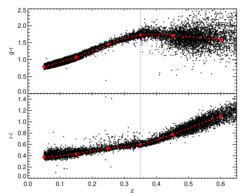
Figure 1.— Sample of red spectroscopic galaxies selected for training in 2000 $\mathrm{deg}^{2}$ of DR8. Top panel shows $g-r$ color and bottom panel $r-i$ color. The red galaxy selection is done in $g-r$ ($r-i$) at $z<0.35$ ($z>0.35$), selecting all galaxies within $2\widetilde{\sigma}_{\mathrm{int}}(z)$ of the spectroscopic redshift of the galaxy. Note that this selection leaves a small number of outliers in the complementary color, as well as a small number of large outliers with anomalously large photometric errors.

6.3. Single Color Member Selection

Having selected our seed galaxies and calibrated a rough initial color–redshift relation, we now proceed to find likely cluster members around each of our seed galaxies. For this first iteration we rely on single-color based membership. Specifically, in R12 we demonstrated that for moderately rich ($\lambda\gtrsim 20$) clusters, one can reliably estimate the red sequence directly from the data as follows. First, we select all galaxies within a color window around the seed galaxy. Next, we fit for the amplitude and tilt of the red-sequence of that galaxy cluster directly from the galaxy data. However, in extending this algorithm to high redshift, we found that large photometric errors can introduce an unacceptable amount of noise in the initial color-box selection of galaxies. Therefore, rather than drawing a color box around the color of the central galaxy for the initial fit, we draw the color box around the model color $\widetilde{c}(z)$ calibrated in the previous section. In detail, we:

1. Take a red galaxy of known spectroscopic redshift (the “seed”).

2. Select all galaxies within $500\,h^{-1}\,\mathrm{kpc}$ of the spectroscopic galaxy, as well as $2\sigma$ of the model color determined in Section 6.2. For the model color, we use $g-r$ at $z\leq 0.35$ and $r-i$ at $z\geq 0.35$. The width $\sigma$ of the color box is set to $0.05$ and $0.03$ respectively, which we expect to be the approximate red sequence width (e.g., R12).

3. Fit the red sequence (slope and intercept) of these galaxies.

4. Measure the single-color $\lambda_{\mathrm{col}}$ using the method of R12 and a fixed aperture of $500\,h^{-1}\,\mathrm{kpc}$.

5. For all overdensities with $\lambda_{\mathrm{col}}>10$, take the galaxies with non-zero $p_{\mathrm{mem}}$ and assign them the spectroscopic redshift of the initial seed galaxy. In practice, we limit our analysis to those galaxies with $p_{\mathrm{mem}}>0.7$.

At this point, we have leveraged the spectroscopic seed galaxies to generate a set of red galaxies as faint as $0.2L_{*}$ over the redshift range of interest. Although not all of these galaxies are true cluster members, we have an estimate $p_{\mathrm{mem}}$ of the probability that each such galaxy is indeed a red sequence cluster member, as in Eqn. 1. Consequently, we can model the contamination of non-red-sequence galaxies in our sample, as shown below.

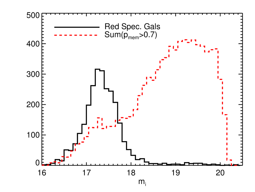
Figure 2.— Magnitude distribution of the red spectroscopic seed galaxies (black histogram) and photometrically selected cluster galaxies with $p_{\mathrm{mem}}>0.7$ (red dashed histogram) in the redshift slice $z\in[0.24,0.26]$. The “cluster member” histogram weights each galaxy by its membership probability. The gain in the training sample of faint red-sequence galaxies through our photometric selection is of critical importance for an accurate calibration of the red-sequence as a function of redshift, particularly at the faint end.

We emphasize that it is essential that we leverage our spectroscopic redshifts to fainter magnitudes to properly model the red sequence. In the case of DR8, our initial seed galaxy sample is comprised of $42,000$ galaxies associated with $\lambda>5$ clusters, almost all of which are preferentially bright. By contrast, our final calibration sample (see Section 6.5) is comprised of over $600,000$ red-sequence galaxies that extend to much fainter magnitudes. This is illustrated in Figure 2. The magnitude distribution of our seed galaxies in the redshift slice $z\in[0.24,0.26]$ (solid black histogram) is contrasted with the membership-weighted magnitude distribution of our final photometrically selected training sample (red dashed histogram). We see that the gain in the effective number of red sequence training galaxies is enormous, allowing for an accurate calibration of the red-sequence (amplitude, tilt, and scatter) as a function of redshift. We have explicitly verified that modest changes to the cuts applied in this section do not impact our final calibration of the red-sequence resulting from the subsequent analysis described in the next section.

6.4. Modeling The Red Sequence

Given a list of galaxies with multidimensional color ($\mathbf{c}$), redshift ($z$, taken to be the cluster redshift), and membership probability ($p_{\mathrm{mem}}$), we can now proceed to calibrate the full red sequence model. Our model is well motivated by observations of galaxy clusters, in that the red sequence at any given redshift in a given color can be described by a simple linear relation between color and $i$-band magnitude $m_{i}$ with intrinsic scatter $\sigma_{\mathrm{int}}$. For example, Figure 3 shows the composite red sequence at $z=0.25$ for both $g-r$ and $r-i$ colors, for all galaxies selected in the final calibration iteration with $p_{\mathrm{mem}}>0.9$.

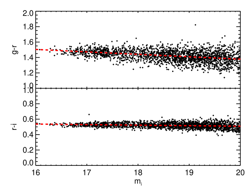
Figure 3.— Composite red sequence at $0.25<z<0.26$ for color-selected galaxies with $p_{\mathrm{mem}}>0.9$. A linear model (red dashed line) with roughly constant intrinsic scatter is a good representation of the red sequence in both $g-r$ and $r-i$. We note that the $p_{\mathrm{mem}}>0.9$ cut is employed for illustration purposes only.

Our red-sequence model we is defined in terms of smoothly evolving functions of redshift characterizing the amplitude and slope of the mean color–redshift relation, and the corresponding covariance matrices. We have opted to use a cubic spline interpolation to parameterize these functions. Given the large number of colors (four for SDSS), and broad redshift range, our model necessarily contains a large number of free parameters. For instance, in our SDSS DR8 implementation, we required a total of 118 parameters to fully characterize the red-sequence model. In principle, we would like to fit the full red sequence model simultaneously. However, to make the problem more tractable we fit the red sequence parameters governing the mean relation and the diagonal elements of the covariance matrix one color at a time. Once these terms are in place, we fit the off-diagonal terms of the covariance matrix. We are also cautious that our model does not have too many free parameters given the training data such that over-fitting becomes possible. As shown in Appendix B, this can be a problem in the case of very sparse training data.

An additional complication comes from the fact that our selection of red sequence galaxies is not entirely clean. Our fit of the red sequence must take into account the background density of non-member galaxies, as described below. In addition, we also have to contend with blue cluster galaxies that are not taken into account by a global background term. These blue galaxies will tend to have two effects. First, as the blue fraction increases at lower luminosities, they will tend to steepen the apparent red sequence tilt. Second, the blend of red and blue galaxies will tend to broaden the apparent intrinsic width of the red sequence.

In order to deal with both of these effects of blue cluster galaxies, we have taken a pragmatic approach. When fitting the red sequence for a given color, we first perform a sharp color cut to concentrate on the core of the red galaxy distribution. Naively, this cut would introduce biases in the recovered red-sequence model, leading to under-estimates of the scatter. We avoid this difficulty by explicitly modeling such a color cut into our likelihood function. All that remains is to specify the color cut. Here, we apply a color cut of $1.5\sigma$ about the median color of the high probability member galaxies, where $\sigma$ is the median absolute deviation of the color about the median.

6.4.1 Measuring the Model Mean and Color Scatter

As noted above, we begin by measuring the model color $\left\langle c|m_{i},z\right\rangle$ as a function of galaxy magnitude $m_{i}$ and cluster redshift $z$ for each color, one at a time. The first step in this process is to define the pivot point $\widetilde{m_{i}}(z)$ used to calibrate the amplitude and tilt of the mean red sequence relation at redshift $z$. We write

$$\left<c|z,m_{i}\right>=\bar{c}(z)+\bar{s}(z)[m_{i}-\widetilde{m_{i}}(z)],$$ (29)

We wish to select a pivot point that is characteristic of most cluster members. To do so, starting from our full members list, we apply a $p_{\mathrm{mem}}>0.7$ cut. Using this sub-sample, we minimize the cost function $E$ where

$$E=\sum|m_{i}-\widetilde{m_{i}}(z)|$$ (30)

where $\widetilde{m_{i}}(z)$ is defined via spline interpolation, and the model parameters are the value of $\widetilde{m_{i}}(z)$ at the nodes.

Having defined our pivot point as a function of redshift, we turn to calibrating the amplitude and slope of the mean relation, i.e., $\bar{c}(z)$ and $\bar{s}(z)$ in Eqn. 29. As a first step, we do a rough estimate of the amplitude and scatter, which we will use to isolate the core of the color distribution of member galaxies. These rough estimates for the amplitude and scatter are denoted $\widetilde{c}(z)$ and $\widetilde{\sigma}(z)$, and are obtained by selecting galaxies with $p_{\mathrm{mem}}>0.7$, and then fitting for these functions as was done in Section 6.2. Specifically, the functions are spline interpolated, with model parameters being the value of these functions at the nodes. The best fit parameters are found by minimizing Eqn. 27, and $\widetilde{\sigma}(z)$ is defined by minimizing Eqn. 28. The primary difference between these new color estimates and scatter relative to those derived in Section 6.2 is that these parameters are now appropriate to the full red sequence rather than simply the (brightest) spectroscopic galaxies.

We now turn to measuring the actual model parameters defining the amplitude $\bar{c}(z)$, slope $\bar{s}(z)$, and scatter $C_{ii}^{\mathrm{int}}(z)$. As before, we use a cubic spline interpolation to parameterize these smoothly evolving functions of redshift. For DR8, we have chosen to use a node spacing of $0.05$ for $\bar{c}(z)$, $0.1$ for $\bar{s}(z)$, and $0.15$ for $C_{jj}^{\mathrm{int}}(z)$. We have found that a relatively tight spacing is required for $\bar{c}(z)$, as this function can change relatively rapidly at filter transitions. Fortunately, $\bar{c}(z)$ is the most robust parameter, and thus is amenable to smaller node spacings. The slope and scatter are not expected to vary as rapidly, and are also noisier to estimate, so we have chosen wider node spacings. Overall, the calibration is not very sensitive to the node spacings chosen provided there are sufficient calibration galaxies (though see Appendix B).

Starting from the photometrically selected galaxy training set from the previous section, we first apply a color cut $|c-\widetilde{c}(z)|<1.5\widetilde{\sigma}(z)$, which ensures that the red-sequence parameters are based on the core of the red galaxy distribution, and are therefore less likely to be biased by blue galaxies. In our model, the probability that a red-sequence cluster galaxy has a color $c$ is given by a truncated Gaussian distribution,

$$G(c)=\frac{\frac{1}{\sqrt{2\pi}\sigma}e^{-(c-\left<c|z,m_{i}\right>)^{2}/2\sigma^{2}}}{\mbox{erf}\left(\frac{1.5\widetilde{\sigma}(z)}{\sqrt{2}\sigma}\right)},$$ (31)

where the expectation value $\left\langle c|m_{i},z\right\rangle$ is defined in terms of our model functions $\bar{c}(z)$ and $\bar{s}(z)$ as per Eqn. 29, and the scatter $\sigma$ is the sum in quadrature of the intrinsic scatter and the photometric error of the galaxy,

$$\sigma=\sqrt{\sigma^{2}+\sigma_{\mathrm{int}}^{2}(z)},$$ (32)

where $\sigma_{\mathrm{int}}(z)=\sqrt{C_{jj}^{\mathrm{int}}}$ is the intrinsic scatter of the red sequence. The ‘erf’ term in the denominator accounts for the fact that $G(c)$ is truncated at $\widetilde{c}(z)\pm\widetilde{\sigma}(z)$, under the approximation $\bar{c}(z)=\widetilde{c}(z)$. This approximation is only used in the overall normalization of the distribution.

The total probability distribution for all of our calibration galaxies must account for the fact that some of our galaxies are in fact background galaxies, so the full color distribution is given by

$$P(c)=p_{\mathrm{mem}}G(c)+(1-p_{\mathrm{mem}})b(c,m_{i}),$$ (33)

where $b(c,m_{i})$ is the distribution in color and magnitude of galaxies about random points. The shape of the background function is obtained by binning all galaxies in color and magnitude bins and using a CIC algorithm as in Section 4.3.

In the end, our task is to calculate the set of $\bar{c}(z)$, $\bar{s}(z)$, and $C_{jj}^{\mathrm{int}}(z)$ values at the given cubic spline nodes that maximizes the total likelihood given by

$$\ln{\cal{L}}=\sum_{i}\ln P_{i}.$$ (34)

As above, we accomplish this maximization by making use of the downhill-simplex method. The maximum likelihood point defines the model functions $\bar{c}(z)$, $\bar{s}(z)$, and $C_{jj}^{\mathrm{int}}(z)$. We emphasize that the likelihood is explicitly truncated as the data is, so that the recovered scatter is unbiased relative to the full population of cluster member galaxies, as we have confirmed with simple mock red sequences and blue clouds.

In Figure 4 we show the color evolution of red sequence galaxies with $p_{\mathrm{mem}}>0.9$ for the $g-r$ and $r-i$ colors in DR8. The red points indicate the $\bar{c}(z)$ values at the spline node positions, and the long-dashed lines are the smooth interpolation. The short-dashed lines indicate the $3\sigma_{\mathrm{int}}$ range. Note that the colors in the figure are not corrected for red sequence tilt. We caution that the intrinsic width of the red sequence can be wider than naively indicated by the $p_{\mathrm{mem}}>0.9$ galaxies, since high probability galaxies must reside closer to the average red-sequence model.

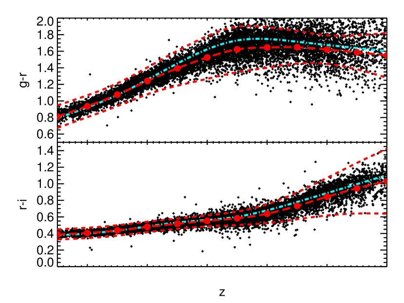
Figure 4.— Color as a function of redshift for the sample of red-sequence galaxies with $p_{\mathrm{mem}}>0.9$. The red points indicate the $\bar{c}(z)$ values at the spline node positions, and the long-dashed lines are the spline interpolation. The short-dashed red lines indicate the $3\sigma_{\mathrm{int}}$ range. Note that the colors in the figure are not corrected for red sequence tilt. The cyan dash-dotted line shows the color model for the bright spectroscopic sample from Figure 1, which tend to be brighter and redder than the full population. We caution that the intrinsic width of the red sequence can be wider than the $p_{\mathrm{mem}}>0.9$ sub-population of galaxies in this illustration suggests, since high probability membership requires the galaxy to fall close to the expected average color. Conversely, the larger number of outliers in $g-r$ above reflects the fact that the photometric errors in $g-r$ at high redshift are larger than the intrinsic width of the red sequence.

6.4.2 Measuring $C_{jk}^{\mathrm{int}}(z)$

With the intercept and slope of the red sequence in hand, as well as the diagonal elements of the covariance matrix, we now estimate the off-diagonal elements of the covariance matrix, $C_{jk}^{\mathrm{int}}(z)$. Once again, we use a cubic spline interpolation, with the same $0.15$ node spacing as used for $C_{jj}^{\mathrm{int}}(z)$.

In order to make the calculation tractable, to constrain the off-diagonal elements of the covariance matrix we consider the problem piecewise, tackling two colors at a time. Each individual piece of the covariance matrix constrained in this way will be positive-definite and thus a valid covariance matrix. Unfortunately, due to noise in the estimation of the parameters, this method does not guarantee that the total covariance matrix, $\mathbf{C}_{\mathrm{int}}(z)$, will also be positive-definite.

To ensure that $\mathbf{C}_{\mathrm{int}}(z)$ is positive-definite, we constrain the parameters for pairs of colors in a specific priority order, ensuring that the best constrained colors have precedence. In the case of DR8 data in the redshift range $z\in[0.05,0.6]$, these are $g-r$ and $r-i$. Then, at each step in the downhill-simplex estimation described below we do not allow any terms in $C_{jk}^{\mathrm{int}}(z)$ that result in a minimum eigenvalue in the total covariance matrix $\mathbf{C}_{\mathrm{int}}(z)$ that is less than $0.01^{2}$. In this way, the first color pair to be constrained ($g-r$,$r-i$) is essentially free, while the final (and noisiest) color pair to be constrained ($u-g$,$i-z$) will not result in a non-invertable covariance matrix $\mathbf{C}_{\mathrm{int}}(z)$.

To perform the pairwise constraints on the off-diagonal elements, let us consider the residuals in two colors $x_{j}$ and $x_{k}$. We start with Eqn. 29,

$$x=c-\left\langle c|m_{i},z\right\rangle=(\bar{c}(z)+\bar{s}(z)[m_{i}-\widetilde{m_{i}}(z)]).$$ (35)

The probability distribution function is again a Gaussian, though this time we explicitly leave the covariance matrix in the equation:

$$G(\mathbf{x})=\frac{1}{\sqrt{2\pi}|\mathbf{C}|^{1/2}}\exp\left[-\frac{1}{2}\mathbf{x}\mathbf{C}^{-1}\mathbf{x}\right],$$ (36)

where $\mathbf{x}=\{x_{j},x_{k}\}$ is the vector of residuals, and the total covariance matrix $\mathbf{C}$ is

$$\mathbf{C}=\mathbf{C}_{\mathrm{int}}(z)+\mathbf{C}_{\mathrm{err}}(z).$$ (37)

Here $\mathbf{C}_{\mathrm{int}}(z)$ and $\mathbf{C}_{\mathrm{err}}(z)$ are the covariance matrices characterizing the intrinsic scatter and photometric error respectively. The intrinsic scatter is simply

$$\mathbf{C}_{\mathrm{int}}=\left(\begin{array}[]{cc}\sigma_{\mathrm{int},j}^{2}&r\sigma_{\mathrm{int},j}\sigma_{\mathrm{int},k}\\ r\sigma_{\mathrm{int},j}\sigma_{\mathrm{int},k}&\sigma_{\mathrm{int},k}^{2}\\ \end{array}\right),$$ (38)

where $\sigma_{j}$ and $\sigma_{k}$ are known from the previous section, and $r$ is the only unknown. The covariance matrix $\mathbf{C}_{\mathrm{err}}(z)$ is derived from the photometric error in each band. Given two colors $c_{j}=m_{\alpha}-m_{\beta}$ and $c_{k}=m_{\gamma}-m_{\delta}$, the covariance matrix characterizing the photometric error is given by

$$\mathbf{C}_{\mathrm{err}}(z)=\left(\begin{array}[]{cc}\sigma_{\alpha}^{2}+\sigma_{\beta}^{2}&\eta\\ \eta&\sigma_{\gamma}^{2}+\sigma_{\delta}^{2}\\ \end{array}\right),$$ (39)

and

$$\eta=\begin{cases}-\sigma_{\beta}^{2}&\text{if $\gamma=\beta$}\\ 0&\text{otherwise}.\end{cases}$$ (40)

Here, we are assuming that neighboring colors are of the form $c_{\alpha\beta}$ and $c_{\gamma\delta}$, i.e., that the “shared” magnitude is $m_{\beta}=m_{\gamma}$. The covariance between photometric errors arises precisely because, for example, the neighboring colors $g-r$ and $r-i$ are both derived from the same $r$-band magnitude.

The color distribution function of the full galaxy population is again given by Eqn. 33, noting that now the background term $b(c_{j},c_{k},m_{i})$ is given by a three dimensional binning in two colors and $i$-band magnitude. In addition, we implement a prior on $r$ with $0$ mean and width $0.45$ for each of the nodes. We find that this prior reduces the noise in the parameter constraints, which is especially important at high redshift where the photometric errors dominate and the covariance matrix is largely unconstrained. At the same time, this prior allows high correlations ($r\sim 0.9$) if strongly favored by the data. Our total likelihood is now given by:

$$\ln{\cal{L}}=\sum_{i}\ln P_{i}-\sum_{n}\frac{(r_{n}/0.45)^{2}}{2},$$ (41)

where $\sum_{n}$ is a sum over all the nodes, and $r_{n}$ is the correlation coefficient at that node. That is, the prior is placed at each of the nodes. Maximization of the likelihood function defines the final values for the correlation coefficients that characterize the intrinsic scatter covariance matrix.

6.5. Iterating The Red-Sequence Model

We emphasize that the estimation of the red sequence parameters in the previous section depends on the membership probabilities ($p_{\mathrm{mem}}$) of the red sequence galaxies. Of course, the membership probabilities themselves depend on the red sequence model. In order to obtain a red sequence model that is consistent with the membership probabilities, we take an iterative approach.

After we calibrate the red sequence parameters based on single color membership probabilities, we run the cluster finder on the training data, as described in Section 9. During these calibration runs we restrict ourselves to finding clusters associated with our seed galaxies so that we can affirmatively associate a spectroscopic redshift with each cluster. We note that our cluster finder starts with the photometric redshift estimate ($z_{\mathrm{red}}$) of each cluster galaxy, so spectroscopic galaxies whose colors are incompatible with the red-sequence at the spectroscopic redshift never result in galaxy clusters. Thus, our training sample at this point results in robust clusters with spectroscopic redshifts. Further, failures in the photoz of the galaxies for red-sequence galaxies are rare (see Figure 7), so any such failures simply slightly reduce the sample of training clusters, without otherwise adversely affecting our training sample. The resulting cluster catalog includes cluster member lists and new membership probability estimates $p_{\mathrm{mem}}$ based on the full color model. With these in hand we can re-estimate the red sequence model as described in Section 6.4.

As we iterate, the largest shifts in the model occur between the first and second iteration, reflecting the shift from estimating membership probabilities based on a single color, and estimating membership probabilities with the full multi-color data. Figure 5 shows the red sequence parameters ($\bar{c}(z)$, $\bar{s}(z)$, and $\sigma_{j}^{\mathrm{int}}$) for each of the first 3 iterations of our red sequence calibration. For illustration, only the figures for the $g-r$ color are shown. The color at the reference magnitude $\widetilde{m_{i}}(z)$ and slopes characterizing the average color of red sequence galaxies converge quickly, and is generally well measured, except for $u-g$ at high redshift, where the large photometric errors in $u$ make our model estimates noisy. The scatter model, on the other hand, converges slowly, particularly at high redshift, where the intrinsic scatter is often sub-dominant to photometric errors. As we now show, however, by the third iteration our model is well converged.

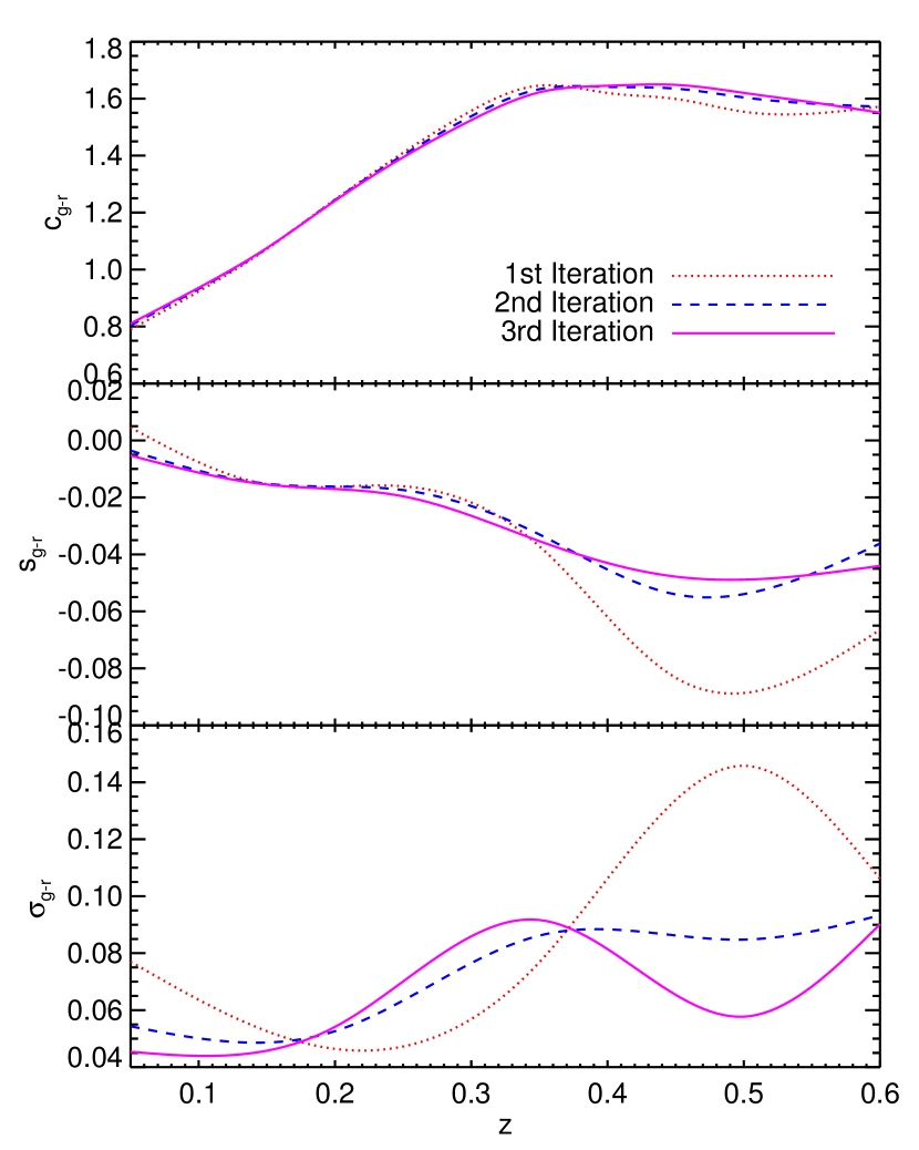
Figure 5.— Top: Average color, $\bar{c}(z)$ for $g-r$, at the pivot magnitude $\widetilde{m_{i}}(z)$, for the first (red dotted line), second (blue dashed line), and third (magenta solid line) iterations of the calibration as a function of redshift. Middle: As for top, with red sequence slope $\bar{s}(z)$. Bottom: As for top, with intrinsic scatter $\sigma_{j}^{\mathrm{int}}=\sqrt{C_{jj}^{\mathrm{int}}}$.

We define convergence of the red sequence model in terms of the relevant quantity for our purposes, i.e., the cluster richness $\lambda$. That is, we require that cluster richness estimates be insensitive to further iterations. To this end, we have run the calibration through ten iterations. Given the red sequence model for each of these ten iterations, we estimate the photometric redshift and cluster richness of a standard set of galaxy clusters while fixing the central galaxy of these systems. Let then $\lambda_{i}$ and $z_{i}$ denote the richness and redshift estimates from iteration $i$. We bin the clusters in narrow redshift slices ($\pm 0.01$), and we calculate: 1- the median ratio $\lambda_{i}/\lambda_{3}$, and 2- the median offset $(\lambda_{i}-\lambda_{3})/\sigma_{3}$, where $\sigma_{3}$ is the error estimate in the richness as estimated from iteration $3$.

In Figure 6 we show the results of these iteration checks for the first 6 iterations in the DR8 training region. Even for the first iteration, for which $p_{\mathrm{mem}}$ was estimated using a single color, the bias is always $<10\%$ (though at the lowest redshift that shift is $\sim 1\sigma$). However, after the third iteration, the biases are always $<1\%$ at low redshift and $<5\%$ at high redshift. The bottom panel shows that after the third iteration the biases are $<0.1\sigma$. Thus, we rely on the output of our third iteration for our final cluster catalog.

Figure 6.— Top: Average richness bias as a function of redshift for the first six iterations of the red-sequence model for the DR8 training region, as compared to $\lambda_{3}$, the richness computed in the third iteration. Even for the first iteration, the bias is $<10\%$ at all redshifts. After the third iteration, the biases are always $<1\%$ at low redshift and $<5\%$ at high redshift. Bottom: Error normalized average deviation relative to the baseline. After the third iteration the bias is always $<0.1\sigma$.

7. Photometric Redshift Estimation

At the end of our calibration we have a complete red sequence model as a function of redshift. Note, however, that in order to estimate the richness of a photometric cluster we need to know the cluster redshift. If we have some initial, reasonably accurate redshift guess $z_{\mathrm{init}}$ for each cluster, we can estimate the cluster richness and determine the high probability cluster members. We then simultaneously fit our red sequence model to all high probability cluster members to derive an improved redshift estimate, and iterate this procedure through convergence. We now describe this full procedure in detail, including the construction of our initial cluster redshift guess $z_{\mathrm{init}}$.

7.1. Redshift Initialization: $z_{\mathrm{red}}$

For the full SDSS DR8 survey, we have multiple photometric redshifts based on large training sets (e.g., Csabai et al. 2007; Sheldon et al. 2012). However, these methods have certain limitations. First, they require training sets that span a broad range of magnitudes, which although abundant at $z\lesssim 0.5$ for SDSS data, will be much sparser at higher redshifts for large surveys such as DES. Second, these methods — in particular $p(z)$ methods such as that of Sheldon et al. (2012) — are very good at estimating the ensemble of redshifts for a broad class of galaxies. However, our needs are much more specific: we wish to have a good initial single-value estimate of the redshift of the central galaxy of galaxy clusters to initialize our cluster photometric redshift estimation procedure. To that end, we have developed our own photometric redshift estimator $z_{\mathrm{red}}$ which is specifically designed to work on red sequence galaxies.

Given a red-sequence galaxy at redshift $z$ with $i$-band magnitude $m_{i}$, color vector $\mathbf{c}$, and photometric error $\mathbf{C}_{\mathrm{err}}(z)$, the probability distribution of its color is simply

$$P(\mathbf{c})\propto\exp\left(-\frac{1}{2}\chi^{2}\right)$$ (42)

where $\chi^{2}$ is given by Eqn. 6, i.e.,

$$\chi^{2}=\left(\mathbf{c}-\left<\mathbf{c}|z,m_{i}\right>\right)\left(\mathbf{C}_{\mathrm{int}}(z)+\mathbf{C}_{\mathrm{err}}(z)\right)^{-1}\left(\mathbf{c}-\left<\mathbf{c}|z,m_{i}\right>\right).$$ (43)

The corresponding log-likelihood is therefore simply $\ln{\cal{L}}=-0.5\chi^{2}$. In practice, we also include an additional volume prior that accounts for the fact that there is more volume at higher redshifts. Assuming that the luminosity function does not evolve over the redshift uncertainties, the probability that a galaxy of a given luminosity is at redshift $z$ is

$$P_{0}(z)\propto\frac{dV}{dz}=(1+z)^{2}D_{A}^{2}(z)cH^{-1}(z),$$ (44)

which leads us to the likelihood

$$\ln{\cal{L}}_{\mathrm{red}}=-\frac{\chi^{2}}{2}+\ln\left|\frac{dV}{dz}\right|.$$ (45)

The redshift estimator $z_{\mathrm{red}}$ is that which maximizes the above likelihood. We use the “red” subscript to indicate that the redshift estimator assumes a red sequence galaxy model. We maximize the likelihood along a redshift grid with $\delta z=0.005$, and then use parabolic interpolation to find the correct maximum. This search is restricted to galaxies with $m_{i}<m_{*}(z)+2.5$, since galaxies fainter than this fall well below the luminosity threshold used to define cluster richness (recall $m_{*}(z)$ is defined in Sec. 4.2). The error estimate for $z_{\mathrm{red}}$ is estimated as the standard deviation of the redshift over its posterior, i.e.

$$\sigma_{z_{\mathrm{red}}}^{2}=\left\langle z^{2}\right\rangle-\left\langle z\right\rangle^{2}$$ (46)

where

$$\left\langle z^{n}\right\rangle=\frac{\int dz\ {\cal{L}}_{\mathrm{red}}(z)z^{n}}{\int dz\ {\cal{L}}_{\mathrm{red}}(z)}.$$ (47)

We could, of course, store the posterior of the redshift distribution, but we have chosen not to do so since the only use of $z_{\mathrm{red}}$ in the redMaPPer algorithm is that of providing an initial redshift estimates for galaxy clusters.

The top-left panel of Figure 7 shows $z_{\mathrm{red}}$ for DR8 cluster training galaxies with $p_{\mathrm{mem}}\geq 0.9$ versus the spectroscopic redshift of the corresponding central galaxy $z_{\mathrm{CG}}$. We see that $z_{\mathrm{red}}$ performs very well, with low bias and scatter, and very few gross outliers. The “flare-up” of the points around $z_{\mathrm{CG}}\sim 0.35$ is due to the $4000\,\mathrm{\AA}$ break moving from the $g-r$ to the $r-i$ color.

The performance of $z_{\mathrm{red}}$ is better illustrated in the bottom-left panel of the same figure. The black triangles show the mean offset $z_{\mathrm{red}}-z_{\mathrm{CG}}$ in redshift bins, the blue dashed line shows the average error in $z_{\mathrm{red}}$ as estimated above, while the red-dashed line shows the observed rms of the redshift offset in each of the redshift bins. The magenta dotted line shows the fraction of $4\sigma$ outliers. It is clear from the figure that our errors are somewhat overestimated, and that there is a small redshift bias in $z_{\mathrm{red}}$.

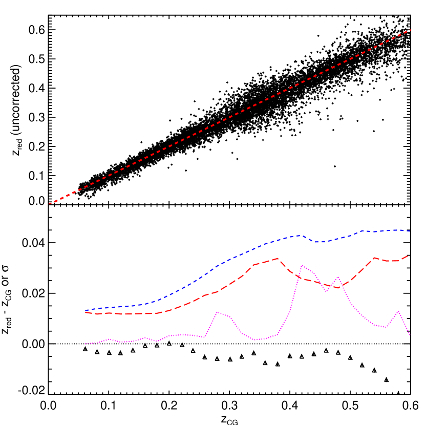
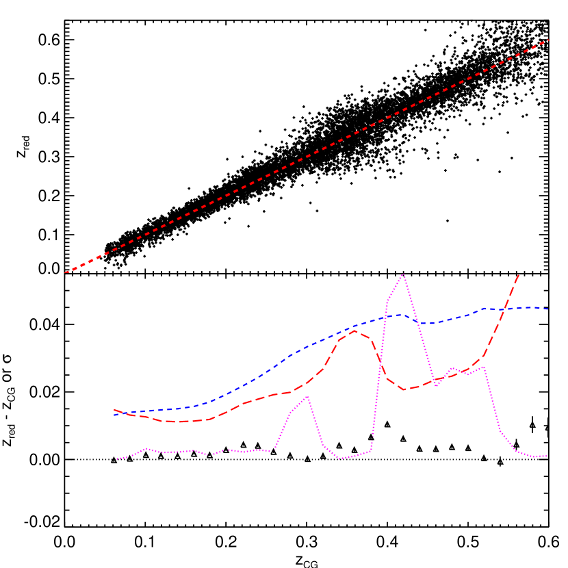
Figure 7.— Left, top: Uncorrected photometric redshift $z_{\mathrm{red}}$ for cluster member galaxies in DR8 with $p_{\mathrm{mem}}>0.9$, as a function of the central galaxy spectroscopic redshift $z_{\mathrm{CG}}$. Left, bottom: The black triangles show the mean redshift offset $z_{\mathrm{red}}-z_{\mathrm{CG}}$ in several redshift bins. The red long-dash line is the rms of these offsets, while the blue short-dash line is the average estimated redshift error. The dotted magenta line is the fraction of $4\sigma$ outliers as a function of redshift. Right, top: Corrected photometric redshift $z_{\mathrm{red}}$, using 49, for cluster member galaxies in DR8, as in left panel. Right, bottom: Bias, scatter, and outlier fraction, as in left panel, now for the corrected redshift.

We correct for the deficiencies revealed in the left panel of Figure 7 by applying an afterburner. Specifically, for the above cluster sample we define the mean redshift offset as a function of redshift,

$$dz(z)=\left\langle(z_{\mathrm{red}}^{0}-z_{\mathrm{CG}})|z_{\mathrm{CG}}\right\rangle$$ (48)

where $z_{\mathrm{red}}^{0}$ is the original, uncorrected redshift estimate defined above. That is, $dz(z)$ is the curve traced by the black triangles in the bottom-left panel of Fig. 7. We define a corrected $z_{\mathrm{red}}$ redshift, as the solution to the equation

$$z_{\mathrm{red}}=z_{\mathrm{red}}^{0}+dz(z_{\mathrm{red}})$$ (49)

In practice, the above treatment is slightly simplified, since our correction afterburner allows for the redshift bias to be a function of magnitude. For details, we refer the reader to Appendix A.1.

In the right panel of Figure 7 we show the corrected value of $z_{\mathrm{red}}$ as a function of $z_{\mathrm{CG}}$ after applying our afterburner, again for a sample of galaxies with $p_{\mathrm{mem}}>0.9$. The notation is the same as for the left panel. The biases are improved at high redshift, although there are still some residual issues at $z\sim 0.4$ where $z_{\mathrm{red}}$ is biased by $\sim 0.3\sigma$. The reason the biases are not completely removed is due to the asymmetric and non-Gaussian nature of the scatter at the filter transition. We also note that the afterburner removes residual biases observed as a function of $m_{i}$ (not shown). The overall small bias and scatter in $z_{\mathrm{red}}$ allows us to use this photometric redshift estimate as a good initial guess with which to initialize our photometric cluster redshift estimator.

7.2. Cluster Redshift Estimation: $z_{\lambda}$

Our approach to computing the cluster photometric redshift $z_{\lambda}$ is essentially an iterative extension of $z_{\mathrm{red}}$. Specifically, given a central galaxy candidate, we:

1. Start with a cluster redshift $z_{\lambda,i}$, where $i$ indexes the iteration. In the first iteration, we set $z_{\lambda,0}=z_{\mathrm{red}}$.

2. Calculate the richness $\lambda$ around the candidate central galaxy setting $z_{\mathrm{cluster}}=z_{\lambda,i}$, and get the associated set of membership probabilities $p_{\mathrm{mem}}$.

3. Select high membership-probability galaxies to estimate a new redshift $z_{\lambda,i+1}$ by maximizing the likelihood function given by Eqn. 51 below.

4. Repeat from step 2 until convergence, such that $|z_{\lambda,i+1}-z_{\lambda,i}|<0.0002$.

All that remains then is the definition of a suitable likelihood function. To begin with, let us assume that we have a sample of known cluster member galaxies. Then, the log-likelihood of the observed colors for these galaxies would be

$$\ln{\cal{L}}=\sum-\frac{\chi^{2}_{i}}{2}-\frac{\ln|{\bf C}|}{2}.$$ (50)

In Eqn. 43 we take into account the log of the determinant of the covariance matrix, $\ln|{\bf C}|$. We have found that, unlike the case of $z_{\mathrm{red}}$, including this term improves the performance of $z_{\lambda}$ when the intrinsic scatter is varying rapidly. This makes sense, given that when utilizing multiple galaxies, one can directly probe the scatter in the red sequence, which is an observable that is inaccessible when estimating single-galaxy photo-$z$s.

Of course, in practice, we do not have a list of known members, but rather a list of likely members with membership probabilities. One might be inclined to adopt a sharp cut $p_{\mathrm{mem}}\geq p_{\mathrm{min}}$ in order to define a likelihood that can be used to estimate the cluster redshift. However, we find that a sharp cut in $p_{\mathrm{mem}}$ leads to numerical instabilities in the iterative process because galaxies can scatter in and out of the sample in the course of the iteration.

To overcome this problem, we adopt instead a soft cut, and define a new likelihood

$$\ln{\cal{L}}=\sum-\frac{w\left[\chi^{2}+\ln|{\bf C}|\right]}{2},$$ (51)

where each galaxy contributes a weight $w$ that smoothly varies from $w=1$ at $p_{\mathrm{mem}}=1$ to $w=0$ at $p_{\mathrm{mem}}=0$.

The assignment of these weights is somewhat ad-hoc. We assume $w(p_{\mathrm{mem}})$ follows a Fermi-Dirac distribution. The transition from $w=0$ to $w=1$ occurs at $p_{70}$, which is the probability threshold that accounts for $70\%$ of the total richness, i.e.,

$$0.7\lambda=\sum_{p_{\mathrm{mem}}\geq p_{70}}p_{\mathrm{mem}}.$$ (52)

The advantage of defining the probability threshold in this way — as opposed to a redshift independent threshold $p_{\mathrm{cut}}$ — is that $p_{70}$ varies with cluster redshift in such a way that one always uses the same fraction of cluster galaxies when estimating redshifts. Were we to take a constant $p_{\mathrm{mem}}$ cut, the number of galaxies contribution to $z_{\lambda}$ would decrease with increasing redshifts, since galaxy $p_{\mathrm{mem}}$ values decrease as the photometry becomes noisier. The width of the distribution is set to $0.04$, which we found is sufficient to regularize the iterative process. Thus, our galaxy weights are defined via

$$w(p_{\mathrm{mem}})=\frac{1}{\exp\left[(p_{70}-p_{\mathrm{mem}})/0.04\right]+1}.$$ (53)

In Figure 8 we illustrate how the iterative process in our redshift estimate works. Fundamentally, each loop in the iteration takes a $z_{\mathrm{in}}$ value for the redshift, and produces a redshift $z_{\mathrm{out}}$, and we wish to find the stable point where $z_{\mathrm{out}}=z_{\mathrm{in}}$. In the figure, we show $z_{\mathrm{out}}(z_{\mathrm{in}})$ for three sample clusters. For the two typical clusters denoted with red short-dashed lines, this function is well behaved, and we quickly achieve convergence. However, there are also $\sim 1\%-2\%$ of clusters that have convergence curves like the blue long-dashed line. These appear to be projection effects between multiple nearby structures. As detailed in Section 9.3, redMaPPer often fragments these clusters along the line-of-sight, as it should. However, which cluster is “dominant” and which is a satellite depends on the initial photometric redshift estimate ($z_{\lambda,0}$).

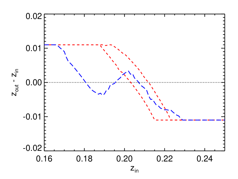
Figure 8.— The redshift difference $z_{\mathrm{out}}-z_{\mathrm{in}}$ for one loop of our iterative photometric redshift estimator, as a function of the input redshift $z_{\mathrm{in}}$. Two typical, well behaved clusters are shown with red short-dashed lines. However, $\sim 1-2\%$ of clusters have convergence curves like the blue long-dashed line. These appear to be projection effects between multiple nearby structures.

Given an estimate for $z_{\lambda}$, we can also map out the posterior $P(z_{\mathrm{true}}|z_{\lambda})$. Defining $\chi^{2}_{\mathrm{norm}}$ via

$$\chi^{2}_{\mathrm{norm}}=\sum w[\chi^{2}+\ln|{\bf C}|]-\mathrm{min}\left(\sum w[\chi^{2}+\ln|{\bf C}|]\right),$$ (54)

we adopt the posterior

$$P(z_{\mathrm{true}}|z_{\lambda})=\frac{\exp(-\chi^{2}_{\mathrm{norm}}/2)\left|dV/dz\right|}{\int d\chi^{2}_{\mathrm{norm}}\exp(-\chi^{2}_{\mathrm{norm}}/2)\left|dV/dz\right|}$$ (55)

where $dV/dz$ is the comoving volume per unit redshift. The above expression defines our estimate of the redshift probability distribution of each cluster. In addition, we fit this distribution with a Gaussian to estimate the redshift error $\sigma_{z_{\lambda}}$.

Finally, in order to ensure that $z_{\lambda}$ is unbiased, we apply an afterburner correction, much in the same way as was done for $z_{\mathrm{red}}$, only now we demand that the redshift be unbiased in the sense that $\left\langle z_{\mathrm{true}}|z_{\lambda}\right\rangle=z_{\lambda}$. We relegate the details to Appendix A.2.

In the top panel in Figure 9 we compare our photometric redshift estimates to the spectroscopic redshift of the central galaxy (where available) for all clusters in DR8 with $\lambda/S(z)>20$ (i.e., every cluster must have 20 galaxy detections). The bottom panel shows the residuals (red triangles), as well as the rms of the distribution (red long-dashed line) and average estimated error $\sigma_{z_{\lambda}}$ (blue short-dashed line). There are small biases that are nevertheless detected with high confidence. We do not yet fully understand the origin of these biases, but intend to return to this problem in a future paper. We see too that there is a feature at $0.35\lesssim z\lesssim 0.45$, both in the bias and scatter, reflecting the additional difficulties introduced by the fact that the $4000\mathrm{\AA}$ break goes from being sampled by $g-r$ to $r-i$. This is also the redshift range where we start running into the limit of the DR8 photometry, which further aggravates these failures. Indeed, these features are greatly reduced when redMaPPer is run on deeper data (e.g., SDSS Stripe 82 coadds, Annis et al. 2011, not shown).

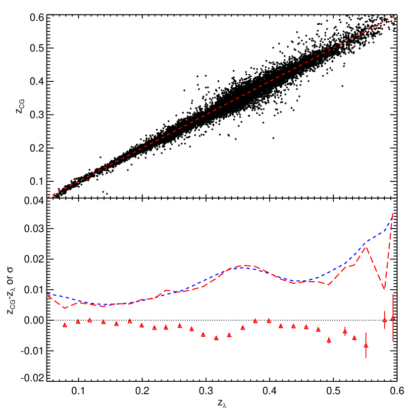
Figure 9.— Top: $z_{\lambda}$ vs. spectroscopic redshift of the assigned cluster central galaxy (CG) for redMaPPer clusters in DR8 with $\lambda/S(z)>20$. Bottom: Red triangles show the mean offset $z_{\lambda}-z_{\mathrm{CG}}$ in various redshift bins. The blue short-dashed line shows the average redshift error on $z_{\lambda}$, while the red long-dashed line shows the measured rms of the redshift offset distribution. The vast majority of outliers are due to errors in cluster centering, i.e., the offset $z_{\lambda}-z_{\mathrm{CG}}$ is large not because $z_{\lambda}$ is incorrect, but rather because the chosen central galaxy is not actually a cluster member.

One interesting thing to note about the top panel in Figure 9 is that the “large” ($\Delta z\sim 0.1$) redshift offsets in this plot do not reflect errors in the cluster redshift estimates, but rather cluster miscentering. That is, when we compare $z_{\lambda}$ to the redshift of the central galaxy, large offsets are primarily due to our selection of a central galaxy that is not, in fact, a cluster member. To demonstrate this, we have created a “clean” sample of clusters where we demand that there be at least two spectroscopic cluster members with $p_{\mathrm{mem}}>0.8$ within $1000\,\mathrm{km}\,\mathrm{s}^{-1}$ of the spectroscopic redshift of central galaxy, thereby ensuring that the central galaxy is in fact a cluster member. Of the $13,178$ redMaPPer clusters in DR8 with spectroscopic redshifts, $1,829$ (or $14\%$) meet this criterion. The corresponding comparison of $z_{\lambda}$ to $z_{\mathrm{CG}}$ in this case is shown in Figure 10. We see that this photometric redshift plot is very clean. The few outliers left ($\lesssim 0.2\%$) are likely multiple systems in projection. In particular, the obvious outlier cluster at $z_{\lambda}\approx 0.22$ correpsonds to the cluster represented by the blue long-dashed line shown in Figure 8.

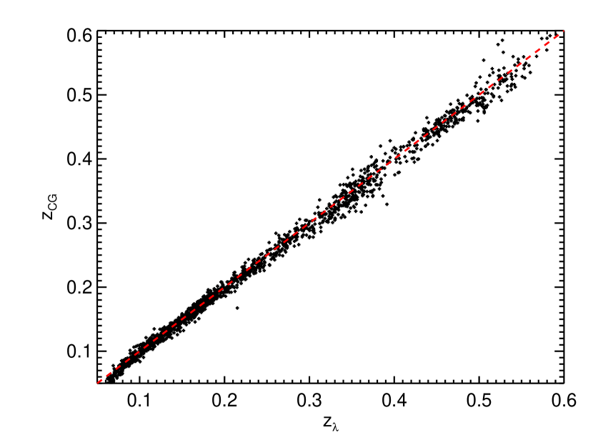
Figure 10.— $z_{\mathrm{CG}}$ vs. $z_{\lambda}$ as in Figure 9, but demanding that the cluster contain at least two cluster members with $p_{\mathrm{mem}}\geq 0.8$ with spectroscopic redshifts within $1000\ \mbox{km/s}$ of the redshift of the assigned central galaxy. This removes clusters centered on non-cluster-member galaxies. Of the $13,178$ redMaPPer clusters in DR8 with spectroscopic redshifts, $1,829$ (or $14\%$) meet this criterion. The few remaining outliers ($\lesssim 0.2\%$) appear to be redshifts failures from multiple systems in projection.

We can get a better sense of the fraction of gross redshift outliers from Figure 11, where we show the fraction of $3\sigma$, $4\sigma$, and $5\sigma$ outliers. A cluster is considered an $N\sigma$ outlier if $|z_{\lambda}-z_{\mathrm{CG}}|\geq N\sigma_{z_{\lambda}}$. To estimate the fraction of outliers as a function of redshift, for each redshift $z$ we collect all clusters with redshift $z_{\lambda}\in[z-0.025,z+0.025]$, and directly measure the fraction of $N\sigma$ outliers. By moving the window $[z-0.025,z+0.025]$ we recover the outlier fraction as a function of redshift. We see that $\approx 1\%$ of our galaxy clusters are $4\sigma$ redshift outliers. We note that the outlier fraction is considerably larger than expected if the errors were simply Gaussian. We emphasize that this fraction is measured using the full cluster sample, not the cleaned version used to produce Figure 10.

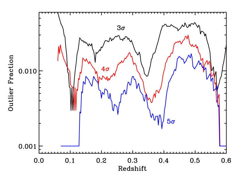
Figure 11.— Fraction of redshift outliers, as a function of photometric cluster redshift. A cluster is said to be an $N\sigma$ outlier if $|z_{\lambda}-z_{\mathrm{CG}}|\geq N\sigma_{z_{\lambda}}$. We show the fraction of $3\sigma$, $4\sigma$, and $5\sigma$ outliers, as labelled. These are computed using the full redMaPPer cluster sample, with no additional spectroscopic requirements on member galaxies (unlike in Fig. 10).

Finally, in Figure 12 we test whether the redMaPPer estimates for the cluster redshift probability distributions $P(z_{\mathrm{true}}|z_{\lambda})$ are accurate. First, we select all clusters with spectroscopic central galaxies to create a “true” $N(z_{\mathrm{CG}})$, shown with a black solid histogram. We note that this is not representative of the full cluster population due to uneven spectroscopic sampling. We compare this to two estimates of $N(z)$ using the same set of clusters. First, we bin clusters using the central values of $z_{\lambda}$, shown with the red-dashed histogram. Second, we integrate $\sum P(z_{\mathrm{true}}|z_{\lambda})$ over the appropriate redshift bins, shown with a yellow band (including the expected measurement errors and Poisson sampling, $\pm 1\sigma$). The red-dashed histrogram is obviously not a good fit to the spectroscopic redshift distribution. In particular, there is an artificial peak near the filter transition at $z=0.35$. This is properly smoothed out by our probability distribution estimate (yellow band), which is a good fit to the spectroscopic data ($\chi^{2}/dof=45.0/40$).

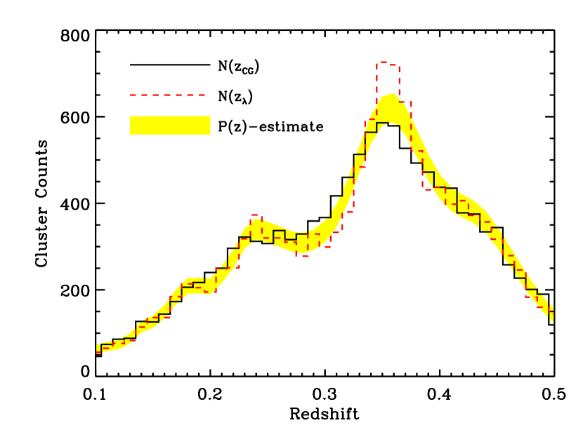
Figure 12.— Comparison of the true and predicted $N(z)$ distribution for redMaPPer DR8 clusters with central galaxies with spectroscopic redshifts and $\lambda/S>20$. We note that this is not representative of the full cluster population due to uneven spectroscopic sampling. The black solid histogram shows the “true” $N(z_{\mathrm{CG}})$. The red-dashed histogram shows the results of binning the central values of $z_{\lambda}$ for the same clusters, leading to obvious biases. The yellow band ($\pm 1\sigma$ errors) shows the results of summing the cluster $P(z)$ values, and provides a good fit to the data.

8. Cluster Centering

The issue of galaxy cluster centering is very important for constraining cosmology with photometric surveys. In particular, miscentered clusters are a leading source of systematic error in stacked weak-lensing mass estimates (e.g., Johnston et al. 2007; Mandelbaum et al. 2008; Rozo et al. 2010), as well as mean velocity dispersions (e.g., Becker et al. 2007). In addition, the cluster richness estimates themselves depend on the choice of center (Lopes et al. 2006). Thus, a well-characterized centering model is essential for precision cosmology.

We assume every galaxy cluster halo has a bright, dominant galaxy residing at its center (e.g., Matthews et al. 1964; Oemler 1976; Schombert 1986; von der Linden et al. 2007, 2012; Menanteau et al. 2013; Mahdavi et al. 2013; Song et al. 2012b; Stott et al. 2012, see also paper II). In our current implementation, we also assume that the central galaxy is red, which is the case for the vast majority of massive clusters. The exceptions are strong cool-core clusters such as Abell 1835 (Allen 1995), where there is enough star formation for the broadband color of the central galaxy to no longer be consistent with that of a red sequence galaxy (e.g., McNamara et al. 2006). Although blue central galaxies are more common (although still rare) at the group scale (e.g., George et al. 2011; More et al. 2011; George et al. 2012; Tinker et al. 2012), the redMaPPer clusters are much more massive than the scale at which this is an issue.

Miscentering of galaxy clusters wherein the central galaxy is undergoing strong star formation is a known failure of the redMaPPer centering algorithm (see Section 8.4 and Paper II). Simply removing the requirement that central galaxies be consistent with the red sequence — i.e. relying solely on luminosity and proximity — can fix some of these clusters, but at the expense of miscentering $\sim 10\%$ of the clusters on foreground galaxies. Likewise, our tests have shown that both galaxy centroids and luminosity weighted galaxy centroids result in worse centering properties than the algorithm currently implemented below (e.g., see also George et al. 2012). Thus, centering on red galaxies is, as far as we can tell, the “least bad” option. In its current implementation, the centering success rate is $\approx 85\%$ (see Paper II). We intend to continue working on improving our centering model for future data releases, as this is currently the dominant source of systematic failures in the redMaPPer cluster catalog.

8.1. Basic Framework

We introduce a fundamentally new way of thinking about identifying the central galaxy of a cluster: rather than specifying a unique cluster center, redMaPPer estimates the probability that a given galaxy is the central galaxy of the cluster. Some clusters have well defined cluster centers, exhibiting a single galaxy with a centering probability $P_{\mathrm{cen}}\approx 1$, whereas others can have two or more reasonable central candidates, with the most likely center having $P_{\mathrm{cen}}\approx 50\%$. We note that these centering probabilities are the angular-position equivalent of the standard photo-$z$ distributions $P(z)$. That is, just as a cluster has an uncertain redshift position characterized by a redshift probability distribution, so too does the cluster have an uncertain angular position on the sky, characterized by the probability of any given galaxy of being the correct cluster center. The importance of this new way of treating cluster centering is that it opens up the possibility of a statistical treatment of cluster centering akin to the statistical treatment of photometric redshifts, allowing us to improve our estimates of the cluster richness functions and cluster correlation functions. A detailed description of this framework will be presented and tested in a future work.

The key insight that allows us to estimate centering probabilities is that there are three different types of galaxies in a cluster: a central galaxy (“CG”), satellite galaxies, and unassociated foreground and background galaxies. Let $\bm{x}$ be an observable vector for a galaxy, e.g., color (via $z_{\mathrm{red}}$), luminosity ($m_{i}$), and position of each galaxy. We define $u_{\mathrm{cen}}$, $u_{\mathrm{sat}}$, and $u_{\mathrm{fg}}$ as the distribution of $\bm{x}$ for central, satellite, and background galaxies respectively. The $u_{\mathrm{cen}}$ and $u_{\mathrm{sat}}$ filters are assumed to depend on cluster redshift and richness, while $u_{\mathrm{fg}}$ depends only on cluster redshift (via $z_{\mathrm{red}}$). We use the subscript “fg” as we expect foreground galaxies will be more likely to be misidentified as CGs. Given a galaxy with observable $\bm{x}$, the probability that it is the central galaxy of a cluster is

$$p_{\mathrm{cen}}(\bm{x}|\lambda,z_{\lambda})=p_{\mathrm{free}}\frac{u_{\mathrm{cen}}}{u_{\mathrm{cen}}+\lambda_{\mathrm{sat}}u_{\mathrm{sat}}+u_{\mathrm{fg}}},$$ (56)

where $p_{\mathrm{free}}$ is the probability that a galaxy has not been partially masked by a higher ranked cluster (as described in Section 9.3; typically $p_{\mathrm{free}}\approx 1$), and $\lambda_{\mathrm{sat}}=\lambda-1$ is the total number of satellite galaxies. This formula can be thought of as the simple definition of probabilities, or it can be interpreted as a Bayesian classification algorithm.

Note, however, that the probability $p_{\mathrm{cen}}$ is not the same thing as the probability $P_{\mathrm{cen}}$ that the galaxy is the unique central galaxy of the cluster. By assumption, there can be only one central galaxy, so if galaxy $i$ is the central galaxy, then every other galaxy $j\neq i$ must not be a central. Consequently, the probability that galaxy $i$ be the central galaxy of a cluster is

$$P_{\mathrm{cen}}\propto p_{\mathrm{cen}}(\bm{x}_{i})\prod_{j\neq i}(1-p_{\mathrm{cen}}(\bm{x}_{j})).$$ (57)

The proportionality constant is set by the condition that there is just one central galaxy in the cluster,

$$1=\sum_{i}P_{\mathrm{cen}}(\bm{x}_{i}).$$ (58)

In addition to the central galaxy probability, we can also calculate the probability that a cluster is centered on a satellite galaxy, given by

$$P_{\mathrm{sat}}=(1-P_{\mathrm{cen}})\frac{\lambda_{\mathrm{sat}}u_{\mathrm{sat}}}{\lambda_{\mathrm{sat}}u_{\mathrm{sat}}+u_{\mathrm{fg}}}$$ (59)

All that remains for us to be able to estimate centering probabilities is the definition of the filters $u_{\mathrm{cen}}$, $u_{\mathrm{sat}}$, and $u_{\mathrm{fg}}$.

8.2. Centering Filters

With the basic formalism laid out, we need to specify the observable $\bm{x}$ and the corresponding filters. There are three observables that we use to select the CG: the galaxy $i$-band magnitude $m_{i}$; the red-sequence photometric redshift $z_{\mathrm{red}}$ of the galaxy; and a weight $w$ that characterizes the local cluster galaxy density around the proposed central galaxy. We also explored replacing our photometric redshift $z_{\mathrm{red}}$ with $\chi^{2}$, the “distance” in color space to the red sequence. However, we have found empirically that $z_{\mathrm{red}}$ works better for estimating central probabilities, in that small amounts of star formation and/or small color errors due to deblending have a much smaller impact on $z_{\mathrm{red}}$ than they do on $\chi^{2}$. We consider each of the filters in turn.

8.2.1 Luminosity Filter: $\phi_{\mathrm{cen}}$

The magnitude of the CG is correlated with both richness and redshift, so we define the CG magnitude filter

$$\phi_{\mathrm{cen}}(m_{i}|\bar{m}_{i},\sigma_{m})=\frac{1}{\sqrt{2\pi}\sigma_{m}}\exp\left(-\frac{(m_{i}-\bar{m}_{i})^{2}}{2\sigma_{m}^{2}}\right),$$ (60)

where in principle both $\bar{m}_{i}$ and $\sigma_{m}$ depend on richness and redshift. In practice, we expect $\sigma_{m}$ to be roughly redshift independent, whereas $\bar{m}_{i}$ obviously depends on redshift. We assume that $\bar{m}_{i}$ traces $m_{*}(z)$, so that the full richness and redshift dependent parameterization of $\bar{m}_{i}$ is

$$\bar{m}_{i}(z_{\lambda},\lambda)=m_{*}(z_{\lambda})+\Delta_{0}+\Delta_{1}\ln\left[\frac{\lambda}{\lambda_{p}}\right],$$ (61)

where $\Delta_{0}$ and $\Delta_{1}$ are redshift independent constants, and $\lambda_{p}$ is the median richness of the sample. Our algorithm for fitting for $\Delta_{0}$ and $\Delta_{1}$ is detailed below.

8.2.2 Photometric Redshift Filter: $G_{\mathrm{cen}}(z_{\mathrm{red}})$

For the photometric redshift filter, we use the red-sequence photometric redshift $z_{\mathrm{red}}$ for each galaxy in the field. We model this as a Gaussian function, with the form:

$$G_{\mathrm{cen}}(z_{\mathrm{red}}|z_{\lambda})=\frac{1}{\sqrt{2\pi}\sigma_{z_{\mathrm{red}}}}\exp\left(\frac{-(z_{\mathrm{red}}-z_{\lambda})^{2}}{2\sigma_{z_{\mathrm{red}}}^{2}}\right).$$ (62)

As the error in the single galaxy photometric redshift dominates that from the cluster photometric redshift, we have set the scatter in $G_{\mathrm{cen}}(z_{\mathrm{red}})$ to that of the individual galaxy. In addition to the photometric redshift filter, we employ a hard cut such $\chi^{2}(z_{\mathrm{red}})<100$ (with 4 degrees of freedom). Investigations of DR8 spectroscopic galaxies have shown that galaxies with $\chi^{2}>100$ are all catastrophic outliers in $z_{\mathrm{red}}$, which is not surprising considering the bad fit to the red-sequence template. By allowing galaxies with $\chi^{2}<100$, we allow some flexibility for galaxies that have slightly offset colors to still be considered as central galaxies. This is especially an issue for SDSS DR8 for bright, nearby central galaxies that may have color shifts caused by deblending problems.

8.2.3 Local Galaxy Density Filter: $f_{\mathrm{cen}}(w)$

The motivation behind the local galaxy density filter is to define an observable $w$ that is a pseudo-gravitational potential connecting each galaxy to every other cluster member. The weight $w$ assigned to a given central candidate is

$$w=\ln\left[\frac{\sum(p_{\mathrm{mem}}(\bm{x}_{i})L_{i}[r_{i}^{2}+r_{c}^{2}]^{-1/2})}{R_{c}(\lambda)^{-1}\sum(p_{\mathrm{mem}}(\bm{x}_{i})L_{i})}\right],$$ (63)

where the sum is over all galaxies within the scale radius $R_{c}(\lambda)$ around the candidate central, $r_{c}=50\,h^{-1}\mathrm{kpc}$ is a core radius used to soften the $1/r$ dependence, $L_{i}$ is each galaxy’s $i$-band luminosity, and $p_{\mathrm{mem}}$ are the usual $\lambda$ membership probabilities. The denominator is chosen to make the argument of the natural log dimensionless, and to remove the obvious dependence of the numerator of $w$ on the total number of terms in the sum. Normalized in this fashion, we expect that $w$ does not scale with cluster richness nor redshift.

We assume that for central galaxies, $w$ follows a log-normal distribution $f_{\mathrm{cen}}(w)$,

$$f_{\mathrm{cen}}(w)=\frac{1}{\sqrt{2\pi}\sigma_{w}}\exp\left[-\frac{(\ln(w)-\bar{w}_{\mathrm{cen}})^{2}}{2\sigma_{w}^{2}}\right].$$ (64)

As noted above, we expect $\bar{w}_{\mathrm{cen}}$ to be richness and redshift independent. On the other hand, $\sigma_{w}$ will certainly depend on richness. The noise in $w$ should scale with raw galaxy counts $(\lambda/S)^{1/2}$, where $S(z)$ is the redshift-dependent factor that relates the raw-galaxy counts to a richness estimate when the survey is not sufficiently deep to reach $0.2L_{*}$ at the redshift of the cluster (see Eqn. 22). For Poisson noise, we set

$$\sigma_{w}=\sigma_{w,\mathrm{cen}}\left(\frac{\lambda}{S\lambda_{p}}\right)^{-1/2}$$ (65)

where $\sigma_{w,\mathrm{cen}}$ is a constant that we fit for. As above, the pivot point $\lambda_{p}$ should be chosen to match the median richness of the sample.

With these definitions, the product

$$u_{\mathrm{cen}}=\phi_{\mathrm{cen}}(m_{i}|z_{\lambda},\lambda)G_{\mathrm{cen}}(z_{\mathrm{red}})f_{\mathrm{cen}}(w|z_{\lambda},\lambda)$$ (66)

is the filter characterizing the distribution of central galaxies.

8.2.4 Satellite Filter: $u_{\mathrm{sat}}$

Satellite galaxies on the red sequence can be described by a filter function analogous to Eqn. 66. Therefore, we have

$$u_{\mathrm{sat}}=\phi_{\mathrm{sat}}(m_{i}|\lambda,m_{*})G_{\mathrm{sat}}(z_{\mathrm{red}})f_{\mathrm{sat}}(w|z_{\lambda},\lambda),$$ (67)

where $f_{\mathrm{sat}}(w)$ is defined in the same way as Eqn. 64, except with parameters appropriate for the satellite galaxies, $\bar{w}_{\mathrm{sat}}$ and $\sigma_{w,\mathrm{sat}}$. The satellite luminosity function, $\phi_{\mathrm{sat}}$, is a Schechter function as described in Eqn. 8. The redshift filter $G_{\mathrm{sat}}(z_{\mathrm{red}})$ is identical to $G_{\mathrm{cen}}(z_{\mathrm{red}})$.

8.2.5 Foreground Filter: $u_{\mathrm{fg}}$

The foreground filter is defined as the expected number of unassociated galaxies within the cluster radius $R_{c}(\lambda)$,

$$u_{\mathrm{fg}}=\bar{\Sigma}_{g,z}(m_{i},z_{\mathrm{red}})f_{\mathrm{fg}}(w)\frac{\pi R_{c}^{2}}{d_{A}^{2}},$$ (68)

where $\bar{\Sigma}_{g,z}$ is the background density per $\mathrm{deg}^{2}$ per $m_{i}$ per $z_{\mathrm{red}}$, calculated in a similar fashion as the red sequence background described in Section 4.3. In addition, the area subtended by the cluster in $\mathrm{Mpc}^{2}$ must be converted to $\mathrm{deg}^{2}$ via the angular diameter distance $d_{A}$, with $d_{A}$ measured in $\mbox{Mpc}/\deg$. Finally, the $f_{\mathrm{fg}}$ filter describes the local galaxy density filter from Eqn. 64, with parameters appropriate for random points ($\bar{w}_{\mathrm{fg}}$ and $\sigma_{w,\mathrm{fg}}$) as described below.

8.3. Implementation

Implementing this formalism requires that we calculate the parameters that describe the filters for central galaxies, satellite galaxies, and foreground/background galaxies. Of course, calibrating these parameters depends on having a training sample to start with. As usual, we approach this problem in an iterative fashion, where the centering model is constrained at the same time as the redMaPPer red-sequence model. In the first iteration, we generate a catalog with roughly correct centering, and use this to provide an initial calibration of the filters. In subsequent iterations we make use of the centering filters and use the output to recalibrate. This procedure is iterated until convergence.

8.3.1 First Iteration and Initial Filter Calibration

First, we implement a rough centering algorithm: for every cluster, we simply select the brightest high probability ($p_{\mathrm{mem}}>0.8$) member galaxy as the central galaxy of the cluster. In this fashion, we obtain a full training catalog with a set of central galaxies that should be roughly correct.

We now use this first iteration of a central galaxy (CG) catalog to determine the filter parameters that we will use in subsequent iterations. Note that because the initial CG catalog contains some miscenterings, when calibrating the CG filters it is important to account for this contamination.

If a cluster is improperly centered on a satellite galaxy, it is most often centered on the brightest satellite. Consequently, the luminosity distribution of satellites which are mistaken as central is not simply a Schechter function ($\phi_{\mathrm{sat}}$). Rather, the luminosity distribution of satellite galaxies in the CG catalog is given by $\phi_{1}(m_{i}|\lambda,m_{*})$, the magnitude distribution of the brightest satellite in clusters of richness $\lambda$. The expected magnitude and $z_{\mathrm{red}}$ distribution of the galaxies in our CG catalog is

$$\begin{split}\rho(m_{i},z_{\mathrm{red}}|z)=&P_{\mathrm{cen}}\phi_{\mathrm{cen}}(m_{i})G(z_{\mathrm{red}}|z)\\ &+P_{\mathrm{sat}}\phi_{1}(m_{i})G(z_{\mathrm{red}}|z)\\ &+(1-P_{\mathrm{cen}}-P_{\mathrm{sat}})\bar{\Sigma}_{g,z}\frac{\pi R_{c}^{2}}{d_{A}^{2}},\end{split}$$ (69)

where $P_{\mathrm{cen}}$ is the probability that the galaxy in question is the central galaxy, as in Eqn. 57, and $P_{\mathrm{sat}}$ is the probability that the cluster is centered on the brightest satellite galaxy. The redshift, $z$, is the spectroscopic redshift of the “seed” galaxy used in the training step.

Our primary goal is to constrain the parameters $\Delta_{0}$, $\Delta_{1}$, and $\sigma_{m}$. However, we also have the parameters $P_{\mathrm{cen}}$ and $P_{\mathrm{sat}}$, which are unknown in the first iteration. For these parameters, we have found that setting them in the first iteration at any reasonable initial estimate ($P_{\mathrm{cen}}\in[0.7,0.9]$; $P_{\mathrm{sat}}\in[0.05,0.2]$) has no marked effect on the final calibration of the filter parameters. Therefore, for simplicity we set $P_{\mathrm{cen}}=0.9$ and $P_{\mathrm{sat}}=0.05$ for each individual cluster in this first iteration.

Before we can continue, we must estimate the parameters for $\phi_{1}(m_{i}|\lambda,m_{*})$. This is modeled as a Gaussian distribution with central value

$$\bar{m}_{\mathrm{sat}}=m_{*}(z)+c_{\phi_{1}}+s_{\phi_{1}}\ln(\lambda/\lambda_{p}),$$ (70)

where $m_{*}(z)$ is obtained from Eqn. 4.2 and $\lambda_{p}$ is the median richness of the sample. The width of the distribution is similarly modeled as

$$\sigma_{\mathrm{sat}}=c_{\sigma,\phi_{1}}+s_{\sigma,\phi_{1}}\ln(\lambda/\lambda_{p}).$$ (71)

The central value must scale with richness because as we sample more galaxies from the luminosity function, we are more likely to find a very bright galaxy. In order to obtain these parameters, we run a simple Monte Carlo with the luminosity function parameters from Section 4.2. For $\alpha=-1.0$ with $\lambda_{p}=30$, we find that $c_{\phi_{i}}=-0.95$, $s_{\phi_{i}}=-0.32$, $c_{\sigma,\phi_{1}}=0.40$, and $s_{\sigma,\phi_{1}}=-0.09$. We note that these parameters depend only on $\alpha$ and $\lambda_{p}$, and thus do not need to be updated in subsequent iterations.

Finally, in order to constrain the parameters $\Delta_{0}$, $\Delta_{1}$, and $\sigma_{m}$, we define our likelihood based on Eqn. 69

$$\ln{\cal{L}}=\sum_{i}\ln\rho(m_{i},z_{\mathrm{red}}|z).$$ (72)

By maximizing this likelihood with respect to $\Delta_{0}$ and $\Delta_{1}$ we can use our training clusters to estimate the $u_{\mathrm{cen}}$ filter parameters.

8.3.2 Calibrating the $w$ Filters

We now turn to calibrating the $w$ filters. We begin by calibrating the foreground and satellite filters, $f_{\mathrm{fg}}(w)$ and $f_{\mathrm{sat}}(w)$. For these purposes we assume that all satellites follow the same spatial profile independent of brightness. Both $f_{\mathrm{fg}}(w)$ and $f_{\mathrm{sat}}(w)$ can be calibrated in a Monte Carlo fashion. We note that foreground galaxies will uniformly sample the cluster area $\pi R_{c}^{2}(\lambda)$, and thus to evaluate $f_{\mathrm{fg}}(w)$ we draw random points uniformly within the disc of every training cluster, and compute the corresponding $f_{\mathrm{fg}}(w)$ parameters, $\bar{w}_{\mathrm{fg}}$ and $\sigma_{w,\mathrm{fg}}$.

The satellite filter $f_{\mathrm{sat}}(w)$ is computed in a similar fashion. First, for every training cluster we randomly select a cluster member with a probability $p$ that is proportional to the membership probability. For this randomly selected member we compute $w$ at the location of that satellite. After computing $w$ for all the training clusters, we compute the corresponding $f_{\mathrm{sat}}(w)$ parameters, $\bar{w}_{\mathrm{sat}}$ and $\sigma_{w,\mathrm{sat}}$.

We can now turn our attention to the distribution $f_{\mathrm{cen}}(w)$. Consider now the distribution $f(w)$ for all central galaxies. This total distribution is then

$$f(w)=P_{\mathrm{cen}}f_{\mathrm{cen}}(w)+P_{\mathrm{sat}}f_{\mathrm{sat}}(w)+(1-P_{\mathrm{cen}}-P_{\mathrm{sat}})f_{\mathrm{fg}}(w).$$ (73)

The only unknowns in this equation are the mean $\bar{w}_{\mathrm{cen}}$ and rms $\sigma_{w,\mathrm{cen}}$ for the central filter, so we write the likelihood

$$\ln{\cal{L}}(\bar{w}_{\mathrm{cen}},\sigma_{w,\mathrm{cen}})=\sum_{i}\ln f(w),$$ (74)

where the sum is over all training clusters. We then maximize this likelihood to find $\bar{w}_{\mathrm{cen}}$ and rms $\sigma_{w,\mathrm{cen}}$.

In Figure 13 we show the central, satellite, and foreground $f(w)$ filters for the final training iteration. It is clear that there is some power here to differentiate between central galaxies and satellites and foregrounds, but it is far from perfect. In particular, satellites are only slightly less well connected than central galaxies.

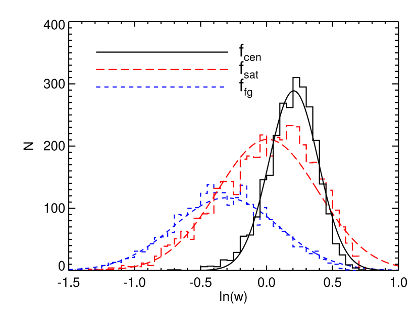
Figure 13.— Histograms of $w$ parameter for central (black solid), satellite (red long-dashed), and foreground/random (blue short-dashed) galaxies. It is clear that there is some power here to differentiate between central galaxies and satellites and foregrounds, but it is not perfect. However, there is some advantage in being able to reject a bright galaxy with a low local density as a likely interloper that does not fit the central galaxy model.

8.3.3 Subsequent Iterations

As noted above, in our first iteration our catalog of CG galaxies is constructed using a simple centering algorithm: i.e., select the brightest high-probability member as the cluster center. In subsequent iterations of the cluster finder calibration we use the probabilistic centering algorithm described in Section 8.1. After application of our centering algorithm we have the important advantage that each cluster now comes tagged with $P_{\mathrm{cen}}$ and $P_{\mathrm{sat}}$. Therefore, we can now repeat the calibrations from Sections 8.3.1 and 8.3.2 while using the correct $P_{\mathrm{cen}}$ and $P_{\mathrm{sat}}$ for each individual galaxy. In this way we continuously improve our centering model with multiple iterations of the cluster finding algorithm.

8.4. A Note on Blue Central Galaxies

At the beginning of this section, we noted that central galaxies undergoing strong star formation pose a particular problem for the redMaPPer centering algorithm. In Figure 14 we show an SDSS image of Abell 1835, a well-known strong cool-core cluster with star formation in the central galaxy. The true center is denoted with a red circle, while the top two candidate redMaPPer centers are circled in blue. As expected, when the color of the central galaxy is far from the red sequence, our centering algorithm instead chooses one of the bright red satellites as a possible center. However, we emphasize that the cluster will not be missing, it will simply be miscentered.

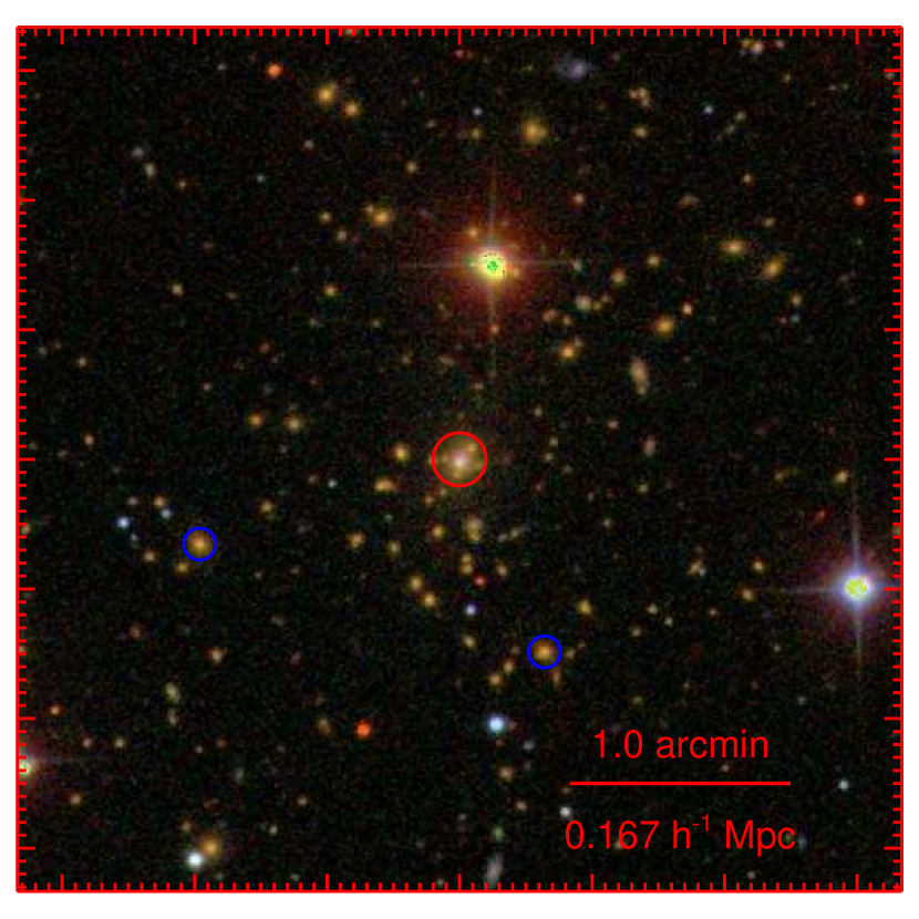
Figure 14.— SDSS image of Abell 1835, a well-known cool-core cluster with strong star formation in the central galaxy (marked with red circle). The two candidate redMaPPer centers are denoted with blue circles, and the true center is missed due to its strong deviation from the red sequence.

We have also made use of SDSS spectra to get an initial estimate on the rate of bad centers due to galaxies that do not agree with our color model (both very blue and very red). We have taken every cluster with a spectroscopic central, and a second brighter spectroscopic galaxy that is within $r<R_{\lambda}$ and $|z_{\mathrm{CG}}-z_{\mathrm{spec}}|<1.5\sigma_{v}$, where $\sigma_{v}$ is the expected velocity dispersion based on the cluster richness (Rozo et al., in prep). If this galaxy is not in the top 5 members list for the cluster, it is considered a possible catastrophic center. In all, $4.6\%$ of the clusters fit this category. Visual inspection of the richest clusters shows that the majority of these galaxies are in the outskirts of the cluster and are not centrals, confirming that the redMaPPer centering algorithm is not simply taking the brightest member as the center. Alternatively, we can look at the subset of these galaxies that are not in the members list and thus were not considered as candidate centrals at all. Only $0.7\%$ of clusters contain such galaxies. From these estimates, we expect the rate of miscentering due to galaxies that are too blue to be selected as central galaxies is $\lesssim 2\%$,

9. The Cluster Finder

We have now described in detail all the ingredients that go into the redMaPPer cluster finder. Here, we focus on how these ingredients are blended within the context of the cluster finder to produce a catalog. In particular, we discuss how clusters are ultimately defined and percolated to ensure that every cluster is found once and only once. From a practical perspective, the cluster finding is broken into three stages. First, we look for overdensities around each individual galaxy using $z_{\mathrm{red}}$ as an estimate of the cluster redshift. Second, we calculate the cluster likelihoods for each of the galaxies that have a sufficient overdensity. Third, after sorting by cluster likelihood, we percolate through the full catalog while probabilistically masking out cluster members. A process flow-chart for reference in this section is shown in Figure 15.

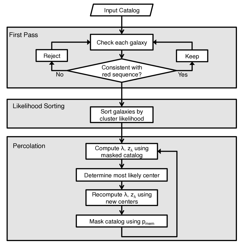
Figure 15.— Process flowchart for the redMaPPer cluster finder, as described in this Section

9.1. First Pass

In the first pass we wish to identify galaxies that are credible centers of galaxy clusters. This task involves a lot of data handling, and so we wish to make it as efficient as possible.

We begin by taking every galaxy in the input catalog with $\chi^{2}(z_{\mathrm{red}})<20$ and brighter than $0.2L_{*}$ at the red-sequence photometric redshift $z_{\mathrm{red}}$. These are very generous cuts, yet they reduce the input DR8 catalog from 56 million galaxies to 23 million possible cluster centers in the redshift region $0.05<z_{\mathrm{red}}<0.6$. Next, we take all galaxies within $0.5h^{-1}\,\mathrm{Mpc}$ of a candidate center and measure $\lambda$, setting the cluster redshift to $z_{\mathrm{red}}$. Candidate centers with $\lambda/S<3$ are rejected. The scale value $S=1/(1-C)$ (from Section 5.1) is used to ensure that we have detected at least three red galaxies above the magnitude limit. This cut rejects a further $\sim 60\%$ of the catalog of candidate centrals. Finally, for all centers that pass these cuts we calculate $z_{\lambda}$ as described in Section 7.2 to better refine the redshift of the possible cluster.

9.2. Likelihood Sorting

Given our list of possible clusters from the first pass, we now calculate the cluster likelihood for each of these clusters. The total likelihood is a combination of the $\lambda$ likelihood and the centering likelihood. To calculate the $\lambda$ likelihood, we first calculate the richness $\lambda$ using the optimized radial scale parameters with $R_{0}=1.0\,h^{-1}\,\mathrm{Mpc}$ and $\beta=0.2$ as described in Section 4. The $\lambda$ likelihood is then given by

$$\ln{\cal{L}}_{\lambda}=-\frac{\lambda}{S}-\sum\ln(1-p_{\mathrm{mem}}),$$ (75)

where $\lambda$ is evaluated at the cluster photometric redshift $z_{\lambda}$.

Next, following Section 8 and Eqn. 66, the centering likelihood is given by

$$\ln{\cal{L}}_{\mathrm{cen}}=\ln[\phi_{\mathrm{cen}}(m_{i}|z_{\lambda},\lambda)G_{\mathrm{cen}}(z_{\mathrm{red}})f_{\mathrm{cen}}(w|z_{\lambda},\lambda)],$$ (76)

where we combine the luminosity, $z_{\mathrm{red}}$, and local galaxy density $w$ of each galaxy. The total likelihood used in the ranking of possible cluster centers is

$$\ln{\cal{L}}=\ln{\cal{L}}_{\lambda}+\ln{\cal{L}}_{\mathrm{cen}}.$$ (77)

Note that the amplitude of the $\lambda$ likelihood function is typically much larger than that of the centering likelihood. Thus, to zeroth order, clusters are first ranked by $\lambda$ likelihood. Two candidate centrals with similar $\lambda$ likelihoods are then ranked according to the central likelihood. As will be described below, we refine the choice of cluster center in the percolation step, so the initial centering likelihood is not especially influential in determining the final cluster center.

9.3. Percolation

Having rank-ordered the cluster candidates according to likelihood, we now need to percolate the list to assign galaxies to clusters and ensure that no cluster is counted multiple times. The basic outline of the percolation proceeds as follows.

1. Given cluster number $i$ in the list, recompute $\lambda$ and $z_{\lambda}$ based on the percolated galaxy catalog. At the beginning of the percolation, the percolated galaxy catalog is simply the input galaxy catalog.

2. Determine the cluster center and centering probability via the method outlined in Section 8.

3. Perform a final calculation of $\lambda$ and $z_{\lambda}$ with respect to the new central galaxy.

4. Update the percolated galaxy catalog by masking out galaxies based on their membership probabilities.

5. Remove all lower-ranked possible centers that have a membership probability $p_{\mathrm{mem}}>0.5$ of being a member of cluster $i$. Note these galaxies are still allowed to provide membership weight to lower-ranked clusters as part of the percolated galaxy catalog.

6. Repeat Step 1 for the next cluster galaxy in the ranked list.

9.3.1 Masking Galaxies

Masking galaxies based on their membership probabilities is the “probabilistic percolation” step of the redMaPPer algorithm. To perform this step, we keep track of the “total probability” that a galaxy belongs to a cluster, which we call $p_{\mathrm{taken}}$. The probability $p_{\mathrm{free}}=1-p_{\mathrm{taken}}$ is the probability that the galaxy does not belong to any cluster. Initially, one has $p_{\mathrm{taken}}=0$ and $p_{\mathrm{free}}=1$ for all galaxies. Upon finding a galaxy cluster, the entire galaxy catalog is percolated by updating the probability $p_{\mathrm{taken}}$ via

$$p_{\mathrm{taken},i+1}=p_{\mathrm{taken},i}+p_{\mathrm{free},i}p_{\mathrm{mem}}$$ (78)

where $p_{\mathrm{mem}}$ is given by Eqn. 1.

Now, when we re-estimate the richness of cluster $i+1$, we must take into account the fact that some of the galaxies have a non-zero probability of belonging to a cluster $j<i+1$. We do so by modifying the richness calculation from Eqn. 2 via

$$\lambda=\sum p_{\mathrm{free}}p_{\mathrm{mem}}(\bm{x}|\lambda).$$ (79)

The first factor above is simply the probability that a galaxy is “free” to belong to the new cluster, and $p_{\mathrm{mem}}$ is the standard membership probability from Eqn. 1. For instance, suppose a galaxy has a probability $p_{\mathrm{mem}}=0.3$ of belonging to the first cluster in the rank-ordered list. In this case, the galaxy still has $70\%$ of its probability to give to a cluster lower in the list. In practice, when quoting cluster membership probabilities $p_{\mathrm{mem}}$ we report not the raw $p_{\mathrm{mem}}$ value as given by Eqn. 1, but rather the product $p_{\mathrm{free}}p_{\mathrm{mem}}$ for that galaxy–cluster pair. That is, the reported value is the correct probability that the given galaxy belongs to the cluster under consideration. For galaxy clusters that are sparse in the sky (e.g., at high richness) these corrections are negligible.

9.3.2 Extent of Clusters and Percolation Radius

As noted above, cluster richness is measured within a radius $R_{c}(\lambda)$ that optimizes the signal-to-noise ratio of the richness measurements (R12), but is not in any way chosen to be related to standard definitions of the extent of a halo, say $R_{200c}$. For cosmological purposes, it is useful to differentiate between the radius $R_{c}(\lambda)$ which defines the richness measurement, and the percolation radius that is used to mask out cluster members and blend or deblend nearby systems. In particular, ideally one selects the percolation radius so that it matches as best as possible the percolation radii employed in the halo definition used to calibrate the corresponding halo mass function.

In the appendix of R12 we used maxBCG clusters to obtain an approximate scaling of mass to $\lambda$ richness. We found that the slope of the mass–$\lambda$ relation is consistent with 1, and that $R_{200c}\approx 1.5R_{c}(\lambda)$. Consequently, we have adopted $1.5R_{c}(\lambda)$ as our default percolation radius. That is, galaxies are masked out to this radius. We note that while galaxies outside the $R_{c}(\lambda)$ radius are not used in the summand in Eqn. 2, we can still estimate $p_{\mathrm{mem}}$ in exactly the same way as we do with all other galaxies out to an arbitrary radius, which is how we implement the large percolation radius above.

In practice, for the $\lambda/S>20$ richness threshold we have employed, changing the mask radius by $\pm 50\%$ has a very small impact on the resulting cluster catalog. Only a small number of clusters ($\sim 5\%$) – primarily satellites of the richest $\lambda>100$ clusters – are affected at all by making this change. We expect to return to the question of what the optimal masking radius is in future work, particularly within the context of cosmological constraints from galaxy clusters.

9.4. A Sample Cluster

At this point, it would be useful to investigate a sample rich cluster to explore the distribution of cluster members. We have selected RM J164019.8+464241.5 (Abell 2219), one of the richest clusters in SDSS, at a redshift of $z=0.23$. In Figure 16 we show four aspects of this cluster. In the top-left panel, we show the SDSS image of the cluster. In the top-right panel, we show the distribution of cluster members with $p_{\mathrm{mem}}>0.05$, with the symbol size proportional to the membership probability. As can be seen in the histogram of $p_{\mathrm{mem}}$ in the bottom-right panel, this distribution is strongly peaked near $p_{\mathrm{mem}}>0.9$. We note that we do not show another, larger peak at $p_{\mathrm{mem}}=0$, for the vast majority of galaxies in the field that are not red-sequence cluster members. Finally, in the bottom-left panel we show the distribution of cluster members as a function of radius. The dashed red line shows the expected distribution of galaxies for an NFW profile with $r_{s}=0.5\,h^{-1}\,\mathrm{Mpc}$, thus showing that the radial distribution of cluster galaxies is broadly consistent with the NFW model.

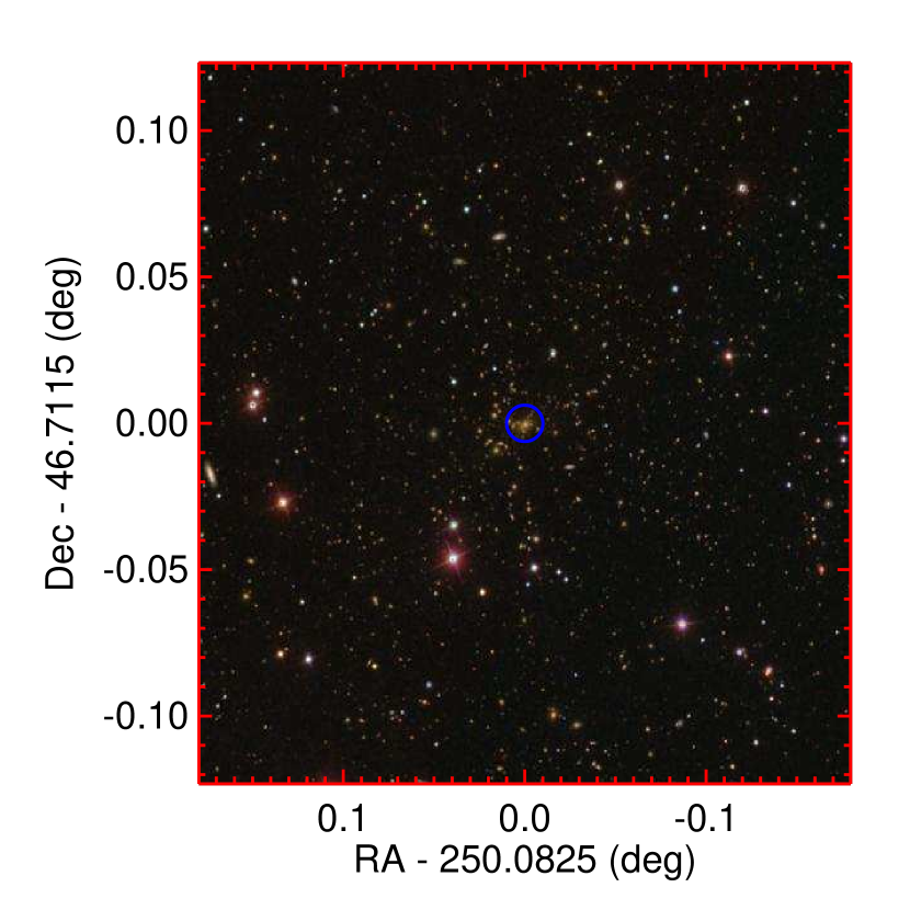
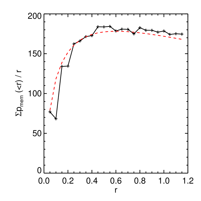
Figure 16.— Top Left: SDSS image of RM J164019.8+464241.5 (Abell 2219). Top Right: Locations of cluster members with $p_{\mathrm{mem}}>0.05$, with the symbol size proportional to the membership probability. Bottom Left: Distribution of cluster members as a function of radius. The dashed red line shows the expected distribution of galaxies for an NFW profile with $r_{s}=0.5\,h^{-1}\,\mathrm{Mpc}$. Bottom Right: Distribution of $p_{\mathrm{mem}}$ for cluster members. This is strongly peaked near $p_{\mathrm{mem}}>0.9$. We note that we do not show another, larger peak at $p_{\mathrm{mem}}=0$, for the vast majority of galaxies in the field that are not red-sequence cluster members.

10. The redMaPPer SDSS DR8 Cluster Catalog

We have run the redMaPPer cluster finding algorithm in the SDSS DR8 photometric catalog described in Sec. 2. The full cluster finder run contains all clusters with $\lambda\geq 5S(z_{\lambda})$ and $z_{\lambda}\in[0.05,0.6]$. However, we have chosen to apply very conservative cuts to our catalog . The cuts we apply are:

1. The richness is cut to $\lambda\geq 20S(z_{\lambda})$. Roughly speaking, this requires that every cluster have at least 20 galaxy counts above the flux limit of the survey or $0.2L_{*}$ at the cluster redshift, whichever is higher. From R12, we estimate that this results in an effective mass cut of $M_{200}\gtrsim 10^{14}\,M_{\sun}$.

2. The redshift range is cut to $z_{\lambda}\in[0.08,0.55]$, so as to minimize edge effects from the training sample.

3. Only clusters with $f_{\mathrm{mask}}<0.2$ are included (see Eqn 23), ensuring clusters are not overly compromised by bad fields, bright stars, and survey edges.

The resulting cluster catalog contains $25,236$ systems. In Figure 17 we show the full footprint of the catalog. The color scale shows the density contrast relative to the mean cluster density, where red regions are denser than average and blue regions are less dense, as estimated using all $\lambda\geq 5$, $z_{\lambda}\in[0.1,0.3]$ clusters so as to give a better sense of the large scale structure in the survey. The image was produced by binning the catalog into a Mangle simple pixelization scheme of depth 7 (Swanson et al. 2008).

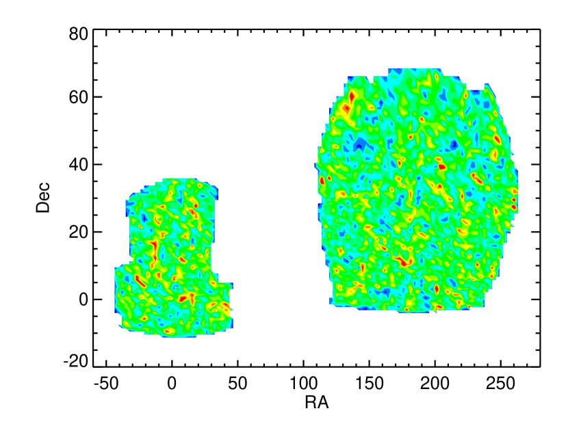
Figure 17.— Footprint of the redMaPPer DR8 catalog, with clusters binned into a Mangle simple pixelization scheme of depth 7. All clusters with $\lambda>5$ and $z_{\lambda}\in[0.1,0.3]$ are shown to better illustrate the large-scale structure in the catalog.

In Figure 18 we show the comoving density of redMaPPer clusters with $\lambda/S(z)>20$ over the full redshift range of interest. The comoving density is roughly constant at $z_{\lambda}\lesssim 0.35$ where the catalog is volume limited. At $z_{\lambda}\sim 0.35$ the richness and redshift scatter are significantly boosted by both the $4000\,\mathrm{\AA}$ break filter transition and the magnitude limit of the survey reaching $0.2L_{*}$. Therefore, the comoving density is boosted by low richness clusters scattering up into our sample. A full accounting for this scatter must be made in order to precisely calculate the redMaPPer abundance function, which we leave to future work. Above this redshift the magnitude limit starts to kick in (via the scale factor $S(z)$), and we only observe the most massive clusters. As an illustration of this effect, in Figure 19 we plot the richness $\lambda$ vs the photometric redshift $z_{\lambda}$ for the final redMaPPer catalog. The red dashed line shows the redshift-dependent richness cut $\lambda>20S(z)$.

Finally, we show a sample redMaPPer cluster. In Figure 20 we show REDM J003208.2+180625.3, the richest redMaPPer cluster not found within the MCXC cluster catalog (Piffaretti et al. 2011), a system with $\lambda=236\pm 12$ at redshift $z_{\lambda}=0.396\pm 0.013$. We note that this cluster is associated with a source in the ROSAT Bright Source Catalog (Voges et al. 1999). The specific data available for each of the clusters and members are described in Appendix G, and a detailed comparison of the redMaPPer clusters to X-ray and SZ catalogs is presented in Paper II.

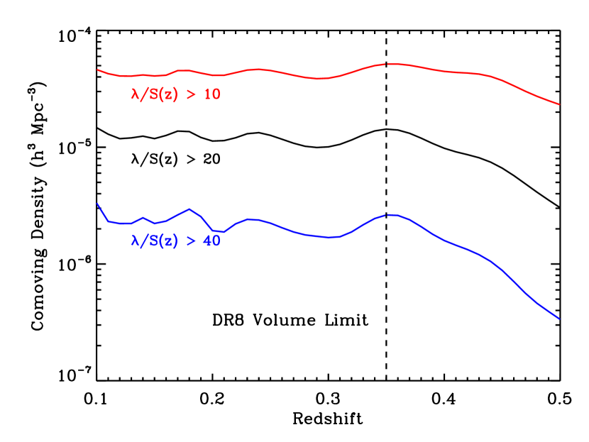
Figure 18.— Comoving density of redMaPPer DR8 clusters as a function of photometric redshift ($z_{\lambda}$) for clusters with $\lambda/S(z)>10,20,40$. All densities have been computed by taking the sum of cluster $p(z)$. The comoving density is roughly constant at $z_{\lambda}<0.35$, where the catalog is volume limited (denoted by the vertical dashed line). Above this redshift the comoving density falls off rapidly as the detection threshold rapidly increases.

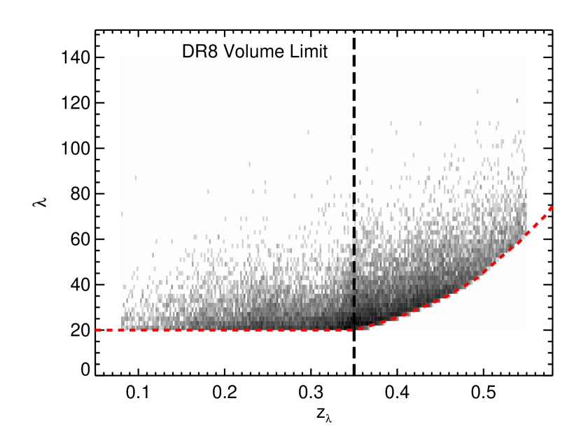
Figure 19.— Two-dimensional histogram of $\lambda$ vs. $z_{\lambda}$ for redMaPPer clusters. The red dashed line shows the redshift-dependent richness cut of $\lambda>20S(z)$. Although this figure generally shows a smooth distribution, the boost in low richness clusters at the transition redshift of $z=0.35$ apparent; this redshift is denoted by the vertical dashed line.

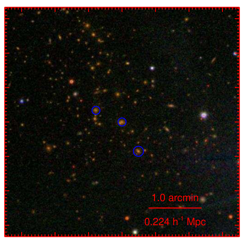
Figure 20.— SDSS composite image of the cluster RM J003208.2+180625.3, the richest redMaPPer cluster not found within the MCXC cluster catalog. This system has $\lambda=236\pm 12$ at a redshift of $z_{\lambda}=0.396\pm 0.013$, and is associated with a source in the ROSAT Bright Source Catalog. This particular cluster has three candidate centers, denoted with blue circles, with $P_{\mathrm{cen}}=\{0.5,0.25,0.25\}$.

11. Purity and Completeness

Purity and completeness can mean many different things depending on the context. There is a tendency to think of purity as the probability that a cluster in the catalog is a real cluster, and to think of completeness as the probability that a real cluster is in the catalog. However, it is often incorrect to think of these quantities as calibrating failure rates of the algorithm. Here, we adopt specific definitions of purity and completeness and discuss their implications. For an alternative definition of purity and completeness by comparing redMaPPer-detected clusters to X-ray catalogs, we refer the reader to Paper II.

For cluster cosmology, the relevant quantity is the probability of detecting a halo of mass $M$ with richness $\lambda_{\mathrm{obs}}$, which can be decomposed into a convolution of two components,

$$P(\lambda_{\mathrm{obs}}|M)=\int d\lambda_{\mathrm{true}}P(\lambda_{\mathrm{obs}}|\lambda_{\mathrm{true}})P(\lambda_{\mathrm{true}}|M).$$ (80)

The probability $P(\lambda_{\mathrm{true}}|M)$ is a feature of the Universe, and must be properly marginalized over in any cosmological study that relies on the cluster number function. Constraining this probability distribution can also be supplemented by utilizing realistic mock catalogs (e.g., Song et al. 2012a, Wechsler et al., in preparation) which we return to in future work. On the other hand, $P(\lambda_{\mathrm{obs}}|\lambda_{\mathrm{true}})$ is a feature of the cluster finding algorithm itself. This probability fully contains all of the information associated with measurement error in our catalog. In the present work, we define completeness and purity as specific integrals over this distribution.

Purity and completeness, used as a simple parametrization of $P(\lambda_{\mathrm{obs}}|\lambda_{\mathrm{true}})$, can be estimated in several ways. Perhaps the simplest consists of removing galaxy clusters, randomizing galaxy positions, and then re-inserting galaxy clusters. The cluster finding algorithm can then be rerun, and one can determine which clusters are detected, and how many “false” clusters are detected (e.g., Goto et al. 2002; Koester et al. 2007b; Hao et al. 2010). However, as shown in the literature (Lopes et al. 2004; Rozo et al. 2011), such an algorithm is fundamentally flawed because background galaxies are not uniformly distributed. Consequently, we take a somewhat different approach, as described below.

1. Generate random points: We generate a list of random points uniformly sampling the input survey mask. These points are to be the centers of mock clusters that will be inserted into the data set. This procedure ensures we sample all the systematics in the survey, as well as the effect of masked regions. We note that these locations are not sampled from the DR8 galaxy positions.

2. Sample “true” cluster richness and redshift: Using the full cluster catalog ($\lambda>5$), we randomly sample galaxy clusters to generate pairs of parameters $(\lambda_{\mathrm{true}},z_{\mathrm{true}})$. This ensures our model cluster distribution has the same richness and redshift distribution as the final catalog, including covariances.

3. For each pair of sampled values $(\lambda_{\mathrm{true}},z_{\mathrm{true}})$, assign them a spatial location using a random point from Step 1, and sample galaxies using the cluster model: Using the same method as in Section 5.2, we use Monte Carlo sampling to generate 5000 galaxies with the model radial and luminosity profiles. From this sample of 5000 cluster galaxies, we randomly sample $\lambda_{\mathrm{true}}$ galaxies from within $R_{c}(\lambda_{\mathrm{true}})$, as well as $k\lambda_{\mathrm{true}}$ galaxies from $R_{c}(\lambda_{\mathrm{true}})<r<R_{c}(2\lambda_{\mathrm{true}})$, where $k$ scales with $\lambda_{\mathrm{true}}$ as appropriate for the radial profile. This ensures that our fake clusters do not have artificial hard edges.

4. Measure $\lambda_{\mathrm{obs}}$ for the generated fake cluster at the random location, and repeat 100 times. When measuring $\lambda_{\mathrm{obs}}$, we mask out galaxies according to the bright stars and edges in the survey mask, as well as applying any necessary magnitude limits. We do not, however, make corrections for higher order effects such as blending of galaxies.

In this way, we generate a map over the full sky of the detectability of clusters as a function of redshift and richness, while taking into account the large-scale structure that is already imprinted on the galaxy catalog. This is a more stringent test than a random-background test, but still does not capture the additional effect that correlated large scale structure can have on the galaxy clusters. However, we expect that these additional effects are subdominant: while the correlation length of galaxy clusters can be as large as $\sim 20\ \mbox{Mpc}$, the typical length-scale over which projections are effective is $\sim 100\ \mbox{Mpc}$ or more, so for most of this volume $1+\xi\approx 1$. Roughly speaking, we would expect no more than $20\%$ corrections to our estimated impurity from these effects, so for example, if 5% of our clusters suffer from projection effects in this analysis, it likely that this fraction is underestimated by by $\sim 0.2\times 0.05=1\%$. A more detailed treatment of projection effects will be presented in a future work (see also the discussion on the impact of the background on $\lambda$ in Rozo et al. 2011).

One additional concern with regards to the above test is that the clusters that we input into our data set are produced with the same filters that we used to find galaxy clusters. As discussed in Rykoff et al. (2012), the choice of luminosity and radial filters have negligible impact on the richness measurements. Rozo et al. (2011) also demonstrated that cluster ellipticity is largely irrelevant. Thus, we expect our results to be robust to changes to the cluster model used to generate the inserted clusters. We have verified this by inserting real redMaPPer clusters as above, where the cluster galaxies are sampled from the members list according to their membership probabilities. Our results are nearly identical to those derived from the model clusters above.

In Figure 21 we illustrate how we use the above outputs to define purity and completeness. The figure shows the expectation value $\left<\lambda_{\mathrm{obs}}\right>$ for the observed richness of a galaxy cluster vs. $\lambda_{\mathrm{true}}$ for a narrow redshift slice ($0.2<z<0.22$). Note that although $\lambda_{\mathrm{true}}$ is a fixed value, each cluster has a distribution of $\lambda_{\mathrm{obs}}$, and we have plotted the mean value.

To define completeness, consider the sub-sample of galaxy clusters in some richness bin in $\lambda_{\mathrm{true}}$, e.g., that defined by the vertical red short-dashed lines in Figure 21. The bulk of this cluster sample falls within a tight locus around the $\lambda_{\mathrm{obs}}\approx\lambda_{\mathrm{true}}$ line, with some noise associated with background fluctuations. The mean relation can be measured, including its scatter, using fitting methods robust to outliers (we rely on median statistics). The diagonal red short-dashed lines show the $\pm 4\sigma$ scatter, and points outside this region are gross outliers. We see that all such outliers fall above the main cloud of points: these are projection effects, where we placed a fake galaxy cluster atop an existing richer structure. It is precisely to characterize these outliers that we do not limit our model clusters to avoid the existing structure in the catalog. The completeness $c(\lambda_{\mathrm{true}})$ is defined as the fraction of the non-outlier points to the total number of clusters in the richness bin, i.e., it is the ratio of the number of clusters within the red dashed parallelogram ($\lambda_{\mathrm{obs}}$ is consistent with $\lambda_{\mathrm{true}}$ within the scatter) to the number of clusters in the $\lambda_{\mathrm{true}}$ bin.

Note that with this definition $c(\lambda_{\mathrm{true}})\leq 1$ does not imply that we are missing clusters. Instead, it is simply estimating the fraction of clusters at a given $\lambda_{\mathrm{true}}$ that suffer from severe projection effects. Similarly, for clusters with $\lambda_{\mathrm{true}}$ near the detection threshold, a fraction of these clusters with have $\lambda_{\mathrm{obs}}$ less than the detection threshold. Thus, these clusters are only “missing” due to well understood observational scatter.

Similarly, we can estimate purity by considering clusters in a bin in $\lambda_{\mathrm{obs}}$, e.g., that defined by the blue long-dashed lines in Figure  21. Several of the clusters in this bin are clear outliers compared to their corresponding $\lambda_{\mathrm{true}}$. The fraction of such outliers in the $\lambda_{\mathrm{obs}}$ bin is the impurity. However, we note one additional restriction; that is, we discard all outliers with $\lambda_{\mathrm{obs}}\geq\lambda_{\mathrm{true}}/2$, denoted by the grey region in the figure. We note that in any projection effect, $\lambda_{\mathrm{obs}}=\lambda_{\mathrm{main}}+\lambda_{\mathrm{proj}}$, the richness of the main and projected halo respectively. By definition, the main halo has a richness $\lambda_{\mathrm{main}}\geq\lambda_{\mathrm{obs}}/2$, and we are concerned with calculating the purity of main halos only. Thus, any fake cluster with $\lambda_{\mathrm{true}}\leq\lambda_{\mathrm{obs}}/2$ is necessarily a projection on a real, significantly richer cluster in the catalog and should be discarded in this analysis. As with the completeness calculation, we emphasize that the resulting purity is the fraction of galaxy clusters as a function of the observed richness that suffer from projection effects, and does not represent an absence of galaxies.

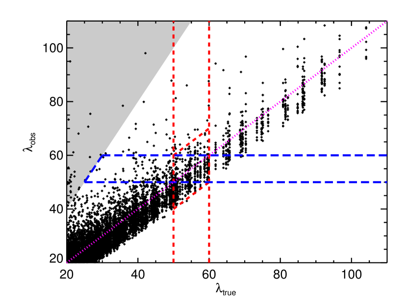
Figure 21.— Expectation value of the measured richness ($\left<\lambda_{\mathrm{obs}}\right>$) vs. input richness ($\lambda_{\mathrm{true}}$) for simulated clusters in the narrow redshift range $0.2<z<0.22$. Note that although $\lambda_{\mathrm{true}}$ is a fixed value, each cluster has a distribution of $\lambda_{\mathrm{obs}}$ and we have plotted the mean value. To measure completeness, we consider the sub-sample of clusters in a richness bin in $\lambda_{\mathrm{true}}$, defined by the vertical red short-dashed lines. While most of the cluster sample falls within a tight locus around $\lambda_{\mathrm{obs}}\approx\lambda_{\mathrm{true}}$, there are some cluster that fall above the $4\sigma$ contours defined by the diagonal red short-dashed lines. These outliers are projection effects, where we placed a fake cluster atop an existing richer structure, and are counted toward incompleteness. For reference, the one-to-one line is shown with the magenta dotted line. To measure purity, we consider the sub-sample of clusters in a richness bin in $\lambda_{\mathrm{obs}}$, defined by the blue long-dashed lines. The clusters that are significant outliers with low $\lambda_{\mathrm{true}}$ are impurities where the measured cluster is the result of a projection effect of multiple systems. The grey region denotes “unphysical” projections where $\lambda_{\mathrm{obs}}\geq 2\lambda_{\mathrm{true}}$, and as such the fake cluster with richness $\lambda_{\mathrm{true}}$ is the secondary rather than the primary halo.

To formalize all of the above discussion, we define the completeness in a bin of richness $\lambda_{\mathrm{true}}$ as

$$\mathrm{completeness}=\frac{\sum\limits_{\mathrm{in\,\lambda_{\mathrm{true}}\,bin}}\int_{\lambda_{0}}^{\lambda_{1}}d\lambda_{\mathrm{obs}}\ P(\lambda_{\mathrm{obs}}|\lambda_{\mathrm{true}})}{N(\lambda_{\mathrm{true}})},$$ (81)

where the sum is over all clusters in a given bin of $\lambda_{\mathrm{true}}$. We define $\lambda_{0}=\lambda_{\mathrm{true}}-4\sigma$, with the restriction that $\lambda_{0}>20$; $\lambda_{1}=\lambda_{\mathrm{true}}+4\sigma$; $\sigma^{2}=\sigma_{\mathrm{int}}^{2}+\sigma_{\lambda}^{2}$; and $N(\lambda_{\mathrm{true}})$ is the total number of clusters in the bin. We estimate $\sigma_{\mathrm{int}}$ directly from the output as the intrinsic scatter in the $\lambda_{\mathrm{obs}}$–$\lambda_{\mathrm{true}}$ relation, and we have chosen to define an outlier (incomplete) cluster as any cluster that has a measured richness $\lambda_{\mathrm{obs}}$ that is more than $4\sigma$ discrepant from its true richness $\lambda_{\mathrm{true}}$.

By the same token, the purity is defined as

$$\mathrm{purity}=\frac{\sum\limits_{\mathrm{in\,\lambda_{\mathrm{obs}}\,bin}}\int_{\lambda_{0}}^{\lambda_{1}}d\lambda_{\mathrm{obs}}\ P(\lambda_{\mathrm{obs}}|\lambda_{\mathrm{true}})}{\sum\limits_{\mathrm{in\,\lambda_{\mathrm{obs}}\,bin}}\int_{\lambda_{\mathrm{obs},1}}^{\lambda_{\mathrm{obs},2}}d\lambda_{\mathrm{obs}}\ P(\lambda_{\mathrm{obs}}|\lambda_{\mathrm{true}})},$$ (82)

where now the sums are over all clusters in a given bin of $\lambda_{\mathrm{obs}}$. Note that we have the additional restruction that the sum is restricted to systems with $\lambda_{\mathrm{true}}\geq\left\langle\lambda_{\mathrm{obs}}\right\rangle/2$. We define $\lambda_{0}=\lambda_{\mathrm{true}}-4\sigma_{\mathrm{int}}$ and $\lambda_{1}=\lambda_{\mathrm{true}}+4\sigma_{\mathrm{int}}$ as before, and $\lambda_{\mathrm{obs},1}$ and $\lambda_{\mathrm{obs},2}$ are the extent of the richness bin in question.

In Figure 22 we show the completeness and purity as a function of richness for five redshift bins for the DR8 galaxy and cluster catalog. At low redshifts ($z<0.3$) the completeness is essentially $\gtrsim 99\%$ at $\lambda>30$, but falls below this threshold due to clusters randomly scattering in and out of the selection threshold. At higher redshift, as we encounter the magnitude limit of the DR8 catalog our richness threshold increases and thus the richness at which these threshold effects come into play also increases.

Our purity is $>95\%$ for all richness and redshift bins, with the richest systems being less pure. This can be understood very simply: consider a chance superposition of two clusters of richness $\lambda$ leading to a single detection of richness $2\lambda$. This factor of two shift has a much more dramatic impact on the overall abundance function at the rich end, simply because the richness function is steeper there, i.e., a constant projection fraction in $\lambda_{\mathrm{true}}$ translates into a projection fraction that decreases with $\lambda_{\mathrm{obs}}$. Again, all these “impurities” actually correspond to real clusters; it’s just that the observed richness has been systematically overestimated.

One curious feature of our purity is that it seems to increase with decreasing richness, and with increasing redshift. This is a consequence of our definition: at lower richness and higher redshifts, the measurements errors in the richness are larger, so a cluster that is a $4\sigma$ outlier needs to be more and more of an extreme projection, which makes such $4\sigma$ outliers rarer. That is, the purity increases not because there are fewer projections, but rather because the projections that do occur become increasingly less important relative to the observational errors in the richness estimates.

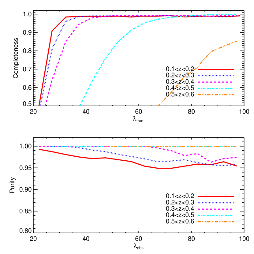
Figure 22.— Top panel: Completeness as a function of input richness, $\lambda_{\mathrm{true}}$, in five redshift bins for the DR8 catalog. At low redshift, the completeness at $\lambda<30$ falls off as measurement errors scatter clusters in and out of our $\lambda\geq 20$ selection threshold. At higher redshifts, the selection threshold increases, as does the measurement error, leading to a broader decrease extending to higher richness values. Bottom panel: Purity — i.e., fraction of galaxy clusters not affected by projection effects — as a function of measured richness, $\lambda_{\mathrm{obs}}$, in five redshift bins.

In this context, it is important to emphasize that the purity that we have defined here is fundamentally different from the purity that is usually defined for X-ray or SZ cluster finding. Let us take SZ as a specific example: a false detection in SZ occurs when random Gaussian noise in the map produces a fluctuation that can be mistaken for an SZ cluster. In our galaxy catalog, galaxies are detected at $>10\sigma$, so a “false detection” of a cluster near our threshold ($\lambda=20$) would require 20 simultaneous $10\sigma$ noise fluctuations colocated in the sky, and strongly correlated across all 5-bands to mimic red-sequence colors. If regions with bad photometry have been properly culled out (by application of the BOSS mask), this simply does not happen. Every galaxy overdensity identified by redMaPPer is a true galaxy overdensity: there are no true false detections driven by observational noise. The key, however, is that the galaxy overdensity is a cylindrical galaxy overdensity which may contain more than one massive halo, and is precisely this rate that we have tried to characterize with our definition of purity.

12. Cluster Masks

One of the great advantages of using model clusters placed randomly on the real sky is that we can use the same output to map the detectability of redMaPPer clusters across the entire survey. In this way, we can directly construct a set of random points directly applicable to the cluster mask, which is not the same as the galaxy mask that defines the survey. An appropriate set of random points is essential for cross-correlation studies for cluster cosmology (e.g., Landy & Szalay 1993).

As an illustration of the difference between the galaxy mask that defines the survey and the cluster mask that defines the redMaPPer catalog, we have run a dense sample of random points in the vicinity of Arcturus using the methods described in Section 11. This very bright star contaminates the SDSS photometry over a large area, and thus effectively masks out a region of the sky that is $0.8^{\circ}$ in radius. To isolate the effect of the survey mask, all the random points shown are associated with model clusters of the same true richness $\lambda_{\mathrm{true}}=40$, with a redshift distribution appropriate for redMaPPer.

In Figure 23 we show the map of the detectability of $\lambda_{\mathrm{true}}=40$ clusters in a $4^{\circ}\times 4^{\circ}$ region around Arcturus. Each pixel shows the fraction of time a sample cluster is detected, using Eqn. 81, where black is $0\%$ and white is $100\%$. In the low redshift bin ($0.1<z<0.2$, upper left panel) the detectability of $\lambda_{\mathrm{true}}=40$ clusters is essentially 100% outside the Arcturus mask, except for a few pixels around bright Tycho stars. Note, however, that due to our requirement that the area of a cluster must not be significantly masked out ($f_{\mathrm{mask}}<0.2$), the edge for the detectability of a cluster at these redshifts is slightly farther from the center of the Arcturus than the edge of the galaxy mask (denoted by the red dashed line). At higher redshift these edges drift closer to each other as the angular extent of the clusters decreases. However, in the highest redshift bin ($0.4<z<0.5$, lower right panel) the cluster is only detected $\sim 60\%\pm 30\%$ of the time (see Figure 22) due to the survey depth. The detectability varies significantly when clusters approach the threshold and we see a strong dependence on the local depth and structure.

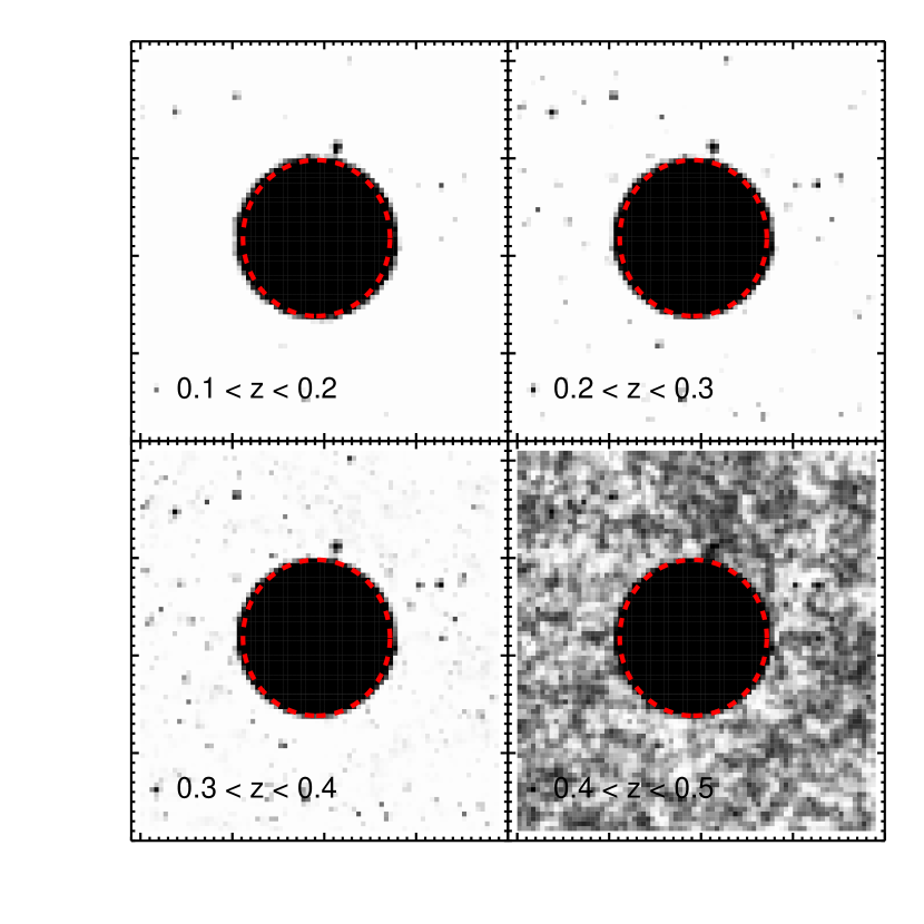
Figure 23.— Map of detectability of redMaPPer clusters of $\lambda_{\mathrm{true}}=40$ in the region of the DR8 galaxy mask in the vicinity of Arcturus (red dashed circle). Each panel is $4^{\circ}$ on a side. At low redshift ($0.1<z<0.2$, upper left panel) a cluster will be detected essentially $100\%$ of the time, except when it falls directly on top of a star (including typical Tycho stars, which show up as small black regions in the plot). Note that due to our requirement than no more than $20\%$ of the area of the cluster is masked out that the effective mask from Arcturus is slightly broader than that of the survey mask. At higher redshift this effect is smaller because the clusters subtend a smaller physical region on the sky. In the $0.4<z<0.5$ bin (lower right panel) the cluster is only detected $\sim 60\%\pm 30\%$ of the time (see Figure 22).

13. Summary

In this paper, we have introduced redMaPPer, a red-sequence cluster finder that is designed to make optimal use of large photometric surveys. As a case study in the implementation of the algorithm, we have run on the SDSS DR8 photometric catalog. We have shown that redMaPPer improves significantly on previous cluster finders (see also Paper II), with many features that will be required to take advantage of upcoming surveys such as DES and LSST. In particular:

1. redMaPPer is based on a multi-color extension of the optimized richness estimator $\lambda$, which has been shown to be a good mass proxy (R12 and Paper II).

2. redMaPPer is self-training, with a modest requirement in the number of training spectra, which can themselves be limited to the brightest cluster galaxies. This makes it particularly well-suited to high-redshift surveys. Furthermore, the multi-color red-sequence model makes optimal use of all color data at all redshifts, with no sharp features as the $4000\,\mathrm{\AA}$ break transitions between filters.

3. redMaPPer can handle complex survey masks. Both mask-corrected richness values can be computed, as well as cluster-appropriate random point catalogs for large-scale structure studies.

4. All clusters are assigned a redshift probability distribution $P(z)$, which enables a more accurate reconstruction of the redshift distribution of the cluster population relative to simple point-redshift estimates.

5. The centering of clusters is fully probabilistic. In this way, the uncertainty in the position of the cluster can be handled in an analagous way to the redshift uncertainty provided by $P(z)$.

6. The algorithm is numerically efficient, and can be run on large surveys with modest computing power.

Using the red-sequence model derived in the redMaPPer calibration phase, we have derived two red-sequence based photometric redshifts. The first, $z_{\mathrm{red}}$, is a red-sequence template-based photo-$z$, that has been designed to generate a good “first-guess” estimation of the redshift in each cluster. We have also shown, in Appendix C, that $z_{\mathrm{red}}$ compares very well to existing DR8 photometric redshifts for this specific class of galaxies. However, $z_{\mathrm{red}}$ has the advantage that it requires many fewer spectroscopic training galaxies. Moreover, these galaxies can be the brightest galaxies in the clusters, with no penalty to the performance of $z_{\mathrm{red}}$ at the faint end of the galaxy sample. The second, $z_{\lambda}$, is a very precise photo-$z$ derived from fitting all cluster members simultaneously to the red sequence model. In addition, we derive a $P(z)$ estimator for $z_{\lambda}$, which we show is superior to point-based photometric redshifts for the purposes of estimating the redshift distribution of the galaxy clusters. In DR8, this is especially true in the region of the filter transition at $z\sim 0.35$.

As a case study in the implementation of the algorithm, we have run redMaPPer on the $10,400\,\mathrm{deg}^{2}$ BOSS region from the SDSS DR8 photometric catalog. Using red galaxy spectroscopic redshifts from 1/5 of the total area from $z\in[0.05,0.6]$, we are able to constrain a robust red-sequence model that defines both the richness and photometric redshift estimators. The photometric redshifts, $z_{\lambda}$, have small bias and low scatter, ranging from $\sigma_{z}=0.006$ at $z\sim 0.1$ to $\sigma_{z}=0.020$ at $z\sim 0.5$, due to increased photometric noise near the survey limit. The rate of catastrophic outliers is low, with only $\sim 1\%$ of galaxy clusters appearing as $4\sigma$ outliers. Note that because of our high photo-$z$ precision, a cluster at $z=0.1$ with a redshift offset as small as $\Delta z=0.025$ is considered a catastrophic redshift failure. Furthermore, we show that the majority of these outliers are bad centers rather than bad redshifts; when the catalog is cleaned by demanding that central and satellite galaxies with spectroscopy must all be within $1,000\ \mbox{km/s}$, the failure rate decreases to $\lesssim 0.2\%$.

After running redMaPPer on the full DR8 photometric catalog, we apply a conservative selection cut of $\lambda/S(z)>20$, for a total of $25,236$ clusters in the redshift range of $z\in[0.08,0.55]$. As shown in paper II, the comoving density of redMaPPer clusters satisfying this cut it lower than that of all other SDSS photometric cluster catalogs. The scale factor, $S(z)$, given by Eqn. 22, defines the correction factor on the richness caused by the survey depth. The catalog is volume-limited at $z<0.35$, where $S=1$ and the survey depth is brighter than the fiducial luminosity cut of $0.2L_{*}$ used by the $\lambda$ richness. Because our selection threshold corresponds to a total of 20 galaxy detections, as we lose galaxies at high redshift due to the magnitude limit of the survey, these 20 galaxies must all be due to bright members. Therefore, the corresponding richness threshold of $20/S(z)$ is much higher. This increased detection threshold results in fewer galaxy clusters at high redshifts. Our adopted richness threshold of 20 detected red sequence galaxies is chosen to provide the most robust cluster catalog possible, with a mass threshold of $M\gtrsim 10^{14}\,M_{\sun}$ where our catalog is volume limited at $z\lesssim 0.35$ (R12, Paper II). Although the full redMaPPer catalog extends to lower richnesses, we expect expect performance will worsen as one moves towards lower and lower richness thresholds.

Finally, we investigate the purity and completeness of our cluster finding algorithm, focusing on the observationally relevant probability distribution $P(\lambda_{\mathrm{obs}}|\lambda_{\mathrm{true}})$. We have defined impurity and incompleteness as the fraction of clusters for which the observed richness $\lambda_{\mathrm{obs}}$ is significantly different from the true richness $\lambda_{\mathrm{true}}$. These outliers are caused by projection effects: when two halos are merged together, this manifests itself as incompleteness — a cluster with richness $\lambda_{\mathrm{true}}$ is up-scattered significantly, so it is “missing” from where it should have been — or impurity — the richness $\lambda_{\mathrm{obs}}$ of such a cluster is significantly overestimated. We note that while the completeness of redMaPPer is near $100\%$, the purity is $\sim 95\%$ at the rich end, increasing at lower richness. This decrease simply reflects larger observational error (in a proportional sense) for lower richness clusters: i.e. “outliers” become more rare not because projection effects are less rare, but because projection effects become sub-dominant to observational uncertainties. Our estimate of the incidence of projection effects is thus $\sim 5\%$, similar to what was estimated in Rozo et al. (2011). A more detailed analysis of projection effects for redMaPPer clusters will be presented in a future work.

In Paper II, we present a detailed comparison of the redMaPPer cluster catalog to various X-ray and SZ catalogs with high quality mass proxies. In all cases, we show that the redMaPPer richness $\lambda$ is a low scatter mass proxy with high completeness and low impurity compared to these “truth” tables. We also compare the performance of redMaPPer to other photometric cluster finders that have been run on SDSS data, and show that redMaPPer outperforms these other algorithms in all metrics (e.g., photo-$z$ performance; mass scatter; and purity and completeness), though some do perform equally well in subsets of these categories in specific redshift ranges.

While this present work has focused on the application of redMaPPer to the SDSS DR8 catalog, we emphasize that this algorithm was developed specifically for upcoming large photometric surveys such as DES and LSST. In particular, its ability to simultaneously utilizes all available photometric data, its smooth handling of the filter transition of the $4000\,\mathrm{\AA}$ break across filter passes, and its ability to self-calibrate using only minimal spectroscopic training samples of bright cluster galaxies are all specifically designed to enable cluster finding in these new photometric data sets. This will be especially advantageous at $z\gtrsim 0.7$ in the Southern Hemisphere, where we do not have the advantages of more than a decade of survey data from the SDSS spectrograph. Thus, in short order we expect redMaPPer will be capable of producing large, high quality catalogs of $\sim 80,000$ clusters at $z<1$ with DES, opening a new era of high redshift cluster cosmology.

Appendix A Photometric Redshift Correction Parameters

A.1. Constraining $z_{\mathrm{red}}$ Correction Parameters

Our approach to constraining the $z_{\mathrm{red}}$ correction parameters $\bar{c}_{z}(z)$ and $\bar{s}_{z}(z)$ is similar to that employed for the red sequence calibration (note the $z$ subscript). As before, we have chosen to constrain these parameters at a given node spacing, using cubic spline interpolation between the nodes. The node spacing we have chosen for DR8 is $0.05$ for $\bar{c}_{z}(z)$ and $0.10$ for $\bar{s}_{z}(z)$, suited to the characteristic variation scales.

One significant complication that we have to deal with is that we have membership probabilities for all the galaxies. In order to properly make use of the probabilities, as in Eqn. 33 we need to know the background PDF. Unfortunately, there is no first-principle way of calculating the $z_{\mathrm{red}}$ background as a function of $z_{\mathrm{true}}$. Therefore, we have chosen to assume the background is a Gaussian function with zero mean and finite width, and to marginalize over this background as a set of nuisance terms. As above, we assume the background width, $\sigma_{b}(z)$ is a smoothly interpolated function with a node spacing of $0.10$. To ensure that we are calculating the correction factors appropriate for red galaxies, and not blue cluster members and interlopers, we limit ourselves to galaxies with $p_{\mathrm{mem}}>0.7$.

Given a model correction,

$$\left<c_{z}|z_{\mathrm{true}},m_{i}\right>=\bar{c}_{z}(z_{\mathrm{true}})+\bar{s}_{z}(z_{\mathrm{true}})[m_{i}-\widetilde{m_{i}}(z)(z_{\mathrm{true}})],$$ (A1)

then we have a Gaussian PDF for the true galaxies,

$$G_{1}=\frac{1}{\sqrt{2\pi}\sigma_{z_{\mathrm{red}}}}\exp\left(\frac{-[(z_{\mathrm{red}}-z_{\mathrm{true}}]-\left<c_{z}|z_{\mathrm{true}},m_{i}\right>]^{2}}{2\sigma_{z_{\mathrm{red}}}^{2}}\right),$$ (A2)

and for the background,

$$G_{2}=\frac{1}{\sqrt{2\pi}\sigma_{b}}\exp\left(\frac{-[z_{\mathrm{red}}-z_{\mathrm{true}}]^{2}}{2\sigma_{b}^{2}}\right).$$ (A3)

The total likelihood is then

$${\cal{L}}=w[p_{\mathrm{mem}}G_{1}+(1-p_{\mathrm{mem}})G_{2}],$$ (A4)

where we have made the addition of a weight function, $w$, which is a smooth function of $\chi^{2}$ that de-weights galaxies with large $\chi^{2}$ and are possible outliers. The weight $w$ is

$$w=\frac{1}{\exp[(\chi^{2}-\chi^{2}_{95})/0.2]+1},$$ (A5)

where $\chi^{2}_{95}$ is the $95^{\mathrm{th}}$ percentile of all galaxies with $p_{\mathrm{mem}}>0.7$.

As before, we find the $\bar{c}_{z}(z)$, $\bar{s}_{z}(z)$, and $\sigma_{b}(z)$ parameters by maximizing $\sum{\cal{L}}$ using the downhill-simplex method.

A.2. Constraining $z_{\lambda}$ Correction Parameters

Our approach to constraining the $z_{\lambda}$ correction parameters is analogous to that used for the $z_{\mathrm{red}}$ parameters in Appendix A.1. However, our job is a little easier because we are applying corrections such that $\left<z_{\mathrm{true}}|z_{\lambda}\right>$ is unbiased rather than the converse. Therefore, the correction term can be a function of $z_{\lambda}$. For DR8, we use a cubic spline interpolation with node spacing of $0.04$ for $\left<c_{z_{\mathrm{true}}}|z_{\lambda}\right>$. In addition, we allow an additional variance term as we find that our raw $z_{\lambda}$ errors are underestimated. For $\sigma_{z_{\lambda},\mathrm{int}}$ we use a smooth function with a node spacing of $0.10$. To ensure that we are using well-measured clusters, we limit ourselves to calibration clusters that have $\lambda/S(z)>10$, where $S$ is the scale factor defined in Eqn. 22. Essentially, this limits us to clusters with at least 10 red galaxies above the luminosity threshold or magnitude limit.

Given a model correction $\left<c_{z_{\mathrm{true}}}|z_{\lambda}\right>$ and intrinsic scatter correction $\sigma_{z_{\lambda},\mathrm{int}}$, we have a Gaussian PDF for the clusters,

$$G=\frac{1}{\sqrt{2\pi}\sigma_{\mathrm{tot}}}\exp\left(\frac{-[(z_{\lambda}-z_{\mathrm{CG}})-\left<c_{z_{\mathrm{true}}}|z_{\lambda}\right>]^{2}}{2\sigma_{\mathrm{tot}}^{2}}\right),$$ (A6)

where $\sigma_{\mathrm{tot}}=\sqrt{\sigma_{z_{\lambda}}^{2}+\sigma_{z_{\lambda},\mathrm{int}}^{2}}$. The total likelihood is then given by $\ln{\cal{L}}=\sum\ln G$. As before, we find $\left<c_{z_{\mathrm{true}}}|z_{\lambda}\right>$ and $\sigma_{z_{\lambda},\mathrm{int}}^{2}$ by maximizing this likelihood using the downhill-simplex method.

With this parametrization in hand, we can calculate the corrected $z_{\lambda}$ and error as $z_{\lambda}=z_{\lambda,\mathrm{raw}}+\left<c_{z_{\mathrm{true}}}|z_{\lambda}\right>$, and $\sigma_{z_{\lambda}}^{2}=\sigma_{z_{\lambda},\mathrm{raw}}^{2}+\sigma_{z_{\lambda},\mathrm{int}}^{2}$. However, we find that after applying these corrections there may still be small residuals in the training sample. Therefore, we iterate on this solution two further times to obtain a final corrected redshift $z_{\lambda}$.

After the calibration is complete, we must also apply these corrections to the $P(z_{\mathrm{true}}|z_{\lambda})$ estimation for each cluster. To replicate the $z_{\lambda}$ offset represented by $\left<c_{z_{\mathrm{true}}}|z_{\lambda}\right>$, we first offset the central value of the $P(z)$ distribution. Next, to replicate the increased scatter we “expand the space” between the $P(z)$ bins, so that a Gaussian fit to $P(z)$ will measure the same width as the corrected $\sigma_{z_{\lambda}}$ value. We find that this does an adequate job of maintaining asymmetries in the $P(z)$ distribution which show up near the filter transitions.

Appendix B How Many Training Clusters?

When calibrating the red sequence in Section 6 on DR8 data, we make use of all the spectroscopy available in our $2000\,\mathrm{deg}^{2}$ training region. However, much of this is superfluous. First, most of the spectroscopic galaxies — even the LRG samples — are not in massive clusters. Second, our strategy of leveraging central galaxy spectroscopy to all the galaxies in a cluster means that we do not require thousands of clusters to perform the calibration. In this section, we investigate how many training clusters — each represented by a single spectroscopic redshift for the central galaxy — are required to create an accurate and unbiased richness and redshift estimate.

To test the number of required training clusters we follow the method of Section 6.5 to measure the bias in the recovered richness and photometric redshift values on a predetermined set of test clusters. For our test suite, we select the $\{5,10,20,40,80\}$ richest clusters per redshift bin of $\pm 0.025$ in the training region. The redshift binning is used to ensure we have a relatively uniform coverage over the redshift range of interest. In practice, of course, the training clusters need not be so uniformly sampled. For each of these spectroscopic training sets we recalibrate the red sequence and measure the richness $\lambda$ and redshift $z_{\lambda}$ for each of the test clusters from Section 6.5.

In Figure 24 we show the results of these test runs. The left panel shows the richness bias and significance of the bias as a function of redshift for the various training samples. Although we can get a reasonable calibration of the red sequence with as few as five spectra per $\pm 0.025$ redshift bin, the resulting richnesses are significantly biased ($\sim 1\sigma$) at the transition redshift $z\sim 0.35$. In order to achieved unbiased richness estimates ($<0.3\sigma$) then we require $\sim 40$ clusters per redshift bin. We assume any residual biases are due to the noise in estimating the off-diagonal elements of the covariance matrix. This results in a total of $\sim 400$ spectra to achieve essentially the same fidelity of calibration as we can achieve with millions of SDSS spectra. The right panel shows the photometric redshift bias and significance, similar to the left panel. For accurate photo-$z$ estimation, we require even fewer training spectra: $\sim 20$ per redshift bin, or a total of 200.

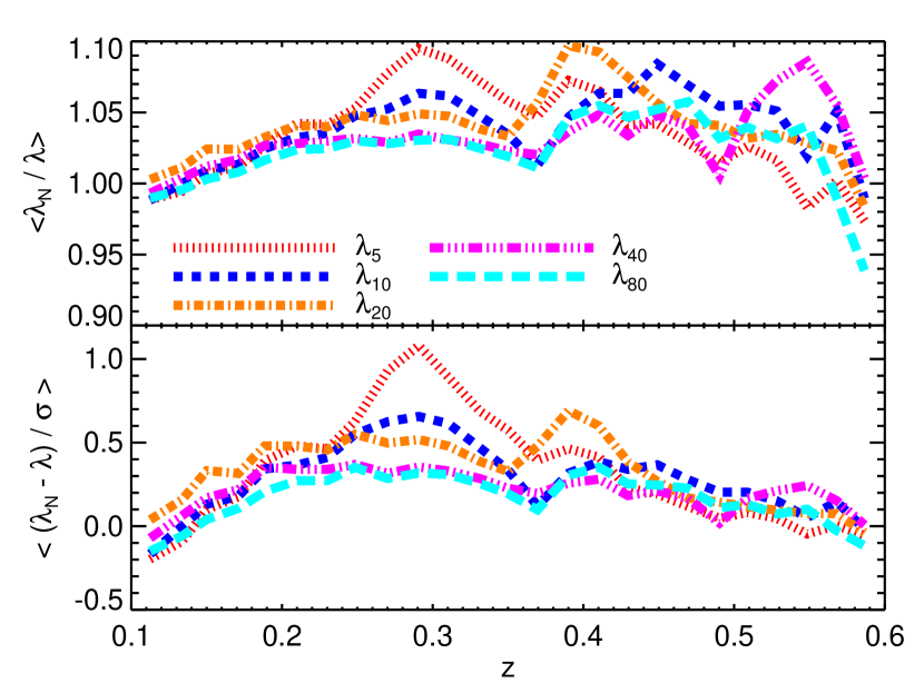
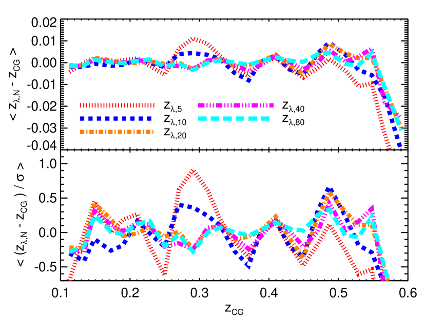
Figure 24.— Left panel, top: Average richness bias as a function of redshift for $\{5,10,20,40,80\}$ training clusters per redshift bin of width $\pm 0.025$, compared to the richness using the full DR8 training sample. All curves use the same set of 4300 test clusters. Left panel, bottom: Error normalized average deviation relative to the baseline. With at least 40 (10) clusters per redshift bin of $\pm 0.025$, biases are always $<0.3\sigma$ ($<0.5\sigma$). Thus, with only 400 well-chosen spectra of the brightest galaxies, we can achieve nearly the same precision as is possible with all the SDSS spectra. Right panel, top: Average uncorrected photometric redshift ($z_{\lambda}$) bias as a function of redshift for $\{5,10,20,40,80\}$ training clusters per redshift bin of width $\pm 0.025$, compared to the spectroscopic redshift of the central galaxy, $z_{\mathrm{CG}}$. Right panel, bottom: Error normalized average deviation relative to the baseline. With at least 20 clusters per redshift bin of $\pm 0.025$ we achieve the same redshift performance as is possible with all SDSS spectra.

For upcoming photometric surveys such as DES, we can obtain these spectra by first running a crude run with an approximate red sequence model. After selecting bright central galaxies, these can easily be followed up spectroscopically, as they are the most luminous galaxies at any redshift. For example, over $85\%$ of the training spectra required for DR8 training are brighter than $m_{i}<18.5$. Thus, our method allows for an incredibly efficient use of limited spectroscopic resources to enable science in large photometric surveys.

Appendix C Comparison of $z_{\mathrm{red}}$ to SDSS DR8 Photo-$z$s

We consider two sets of photometric redshift estimates available for all of DR8. The first, “$z_{\mathrm{photo}}$”, uses an updated method of Csabai et al. (2007), and the second, “$p(z)$”, uses the method of Sheldon et al. (2012). In this section we make use of high probability cluster member galaxies to compare these photometric redshifts to $z_{\mathrm{red}}$ at both bright magnitudes (where training galaxies are plentiful) and at fainter magnitudes.

For our “pseudo-spectroscopic” test sample, we start with all clusters with $\lambda>5$ and a central galaxy with spectroscopic redshift $z_{\mathrm{CG}}$. We then select all members with $p_{\mathrm{mem}}>0.9$. We thus expect a contamination rate of up to 10%, although the real rate should be smaller than this. By assigning each high probability member to the spectroscopic redshift of the central galaxy we can leverage the red sequence to obtain spectroscopic quality redshifts to much fainter magnitudes than available in the SDSS main or LRG spectroscopic samples.

Figure 25 shows the density map of the photometric redshift biases as a function of magnitude for $z_{\mathrm{red}}$, $z_{\mathrm{photo}}$, and $p(z)$ for a narrow redshift slice of $0.195<z_{\mathrm{CG}}<0.205$. For $z_{\mathrm{red}}$ and $z_{\mathrm{photo}}$ we have assumed a probability distribution function (PDF) that is Gaussian with mean $z_{\mathrm{red}}$ ($z_{\mathrm{photo}}$) and width $\sigma_{z_{\mathrm{red}}}$ ($\sigma_{z_{\mathrm{photo}}}$). For the $p(z)$ values we use a spline interpolation to smooth the PDF and normalize the area to unity. On the right-hand side are projected histograms from the density field. The dotted red lines show the $z_{\mathrm{red}}$ distribution for comparison. Note that the density plot clearly shows the separation in magnitude between central and satellite galaxies. Both $z_{\mathrm{red}}$ and $z_{\mathrm{photo}}$ perform well down to the $0.2L_{*}$ limit of the redMaPPer richness estimation, while the $p(z)$ values have a broader distribution at the faint end. These is also obvious structure in the photo-$z$ bias as a function of magnitude.

Figure 26 shows the same map for a narrow redshift slice of $0.395<z_{\mathrm{CG}}<0.405$. While all the photometric redshifts handle the luminous galaxies very well, the appear to be slight biases at the faint end in the case of the DR8 $z_{\mathrm{photo}}$, and a bifurcation of the distribution for the $p(z)$ redshifts. The evolution of the bias in the $p(z)$ estimates is due to a combination of effects. First, the $r$-band magnitude was used as an input to the photo-$z$ estimator. For a field galaxy, a fainter magnitude correlates with a higher redshift. For cluster galaxies, however, galaxies of a wide range of luminosity occupy the same cluster. As a result, when using magnitude-based photo-$z$ estimators on galaxies in clusters, one should expect an increasing bias with magnitude, which is simply a manifestation of the intra-cluster luminosity function. The large width of the error distributions relative to the other estimators are due primarily to the lack of training set galaxies in that range. As discussed in Sheldon et al. (2012), the main focus was on recovering the full $r<21.8$ galaxy sample. To avoid biases induced by training set selection, the authors did not include the most recent BOSS LRG samples in that work and deferred LRG-optimized $p(z)$ estimates to a future paper. It is also worth pointing out that, despite the extra width of the error distributions obtained when using $p(z)$, the recovered redshift distributions obtained by summing the $p(z)$ of Sheldon et al. (2012) are still superior to the distributions estimated using the DR8 $z_{\mathrm{photo}}$ or single-point $z_{\mathrm{red}}$ estimates.

There are two important take-home messages from this comparison. First, the performance of state-of-the-art photo-$z$ estimators appears to be sufficiently accurate for bright galaxies that we would likely be able to use these in the initialization phase of redMaPPer without any loss. Second, $z_{\mathrm{red}}$ appears to be at least as good — if not better — than what is currently achieved, with much smaller spectroscopic training samples. As shown in Appendix B, we can achieve this redshift performance with only $\approx 400$ of the brightest CG spectra. With the technique of assigning the spectroscopic redshift of the central galaxies to the members, we effectively increase the faint end of our training sample. This is very useful for future surveys because of the high cost of obtaining spectroscopic redshifts of faint galaxies.

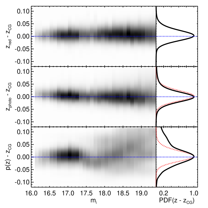
Figure 25.— Top: Density of total $p(z_{\mathrm{red}}-z_{\mathrm{CG}})$ as a function of $i$-band magnitude $m_{i}$ for all cluster members with $p_{\mathrm{mem}}>0.9$ and $0.195<z_{\mathrm{CG}}<0.205$ in clusters with $\lambda>5$. The right panel shows the total PDF at all magnitudes. There is a small bias in $z_{\mathrm{red}}$, though it is constant with magnitude. Middle: Same as top panel, with $z_{\mathrm{photo}}$ calculated with the algorithm of Csabai et al. (2007). The performance is good down to $0.2L_{*}$. The right panel compares the distribution for $z_{\mathrm{photo}}$ (black line) to $z_{\mathrm{red}}$ (red dotted line). Bottom: Same as top panel, with $p(z)$ values from Sheldon et al. (2012). While the bright galaxy performance is good, there are biases at the faint end and the distribution is significantly wider.

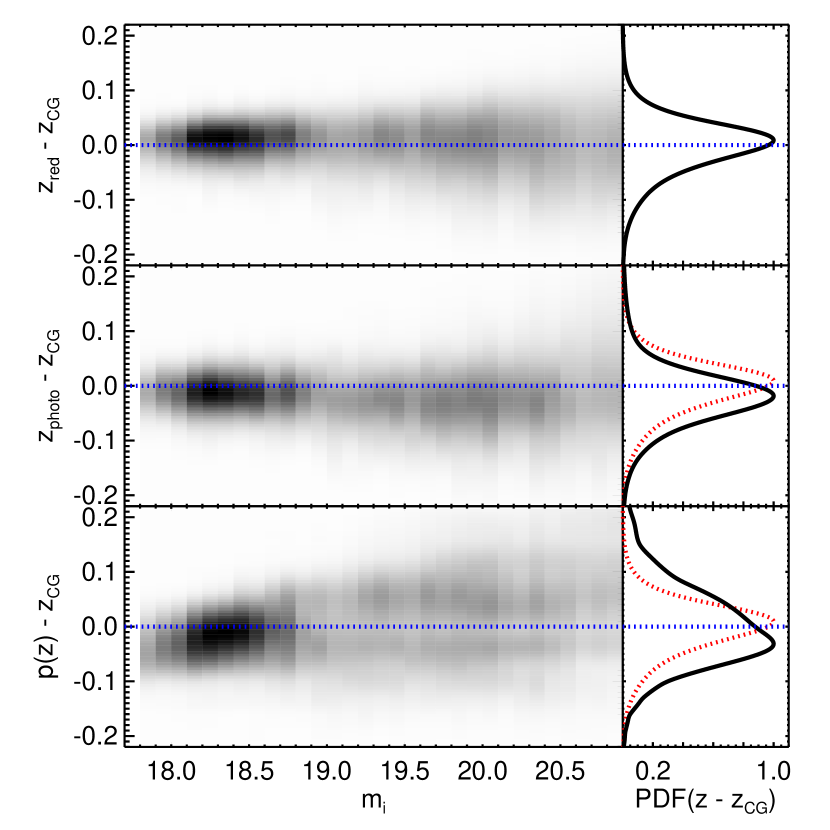
Figure 26.— Same as Figure 25, with members selected from clusters with $0.395<z_{\mathrm{CG}}<0.405$.

Appendix D Computing Performance Benchmarks

The redMaPPer algorithm has been designed to be fast, efficient, flexible, and trivially parallelized. As there are two parts to running redMaPPer, the calibration and cluster-finding stages, we split the performance benchmarks into two parts.

For the calibration phase, the runtime depends on the number of training spectra and clusters. For the DR8 training sample on $2000\,\mathrm{deg}^{2}$, the full calibration takes $\sim 30\,\mathrm{CPU}\,\mathrm{hr}$ on a 3-year old 2.8 GHz AMD Opteron 8389. Current Intel processors can run the calibration roughly twice as fast. For the minimal training sample of 40 clusters per redshift bin (see Appendix B) calibration takes $\sim 13\,\mathrm{CPU}\,\mathrm{hr}$.

The cluster-finding stage is designed to be split into chunks of arbitrary size on the sky. For these purposes we use the Mangle simple pixelization scheme (Swanson et al. 2008), although any pixelization scheme will work. As long as the overlap region between pixels is wider than twice the largest size of any cluster in the catalog, then the percolation of clusters within each cell is guaranteed to be unique. For the DR8 catalog, this corresponds to a border region of $1.5^{\circ}$, corresponding to twice the size of a cluster of richness $\sim 300$ at $z=0.05$, given the mask radius parameters. In total, running the cluster finder on the full DR8 catalog requires $\sim 500\,\mathrm{CPU}\,\mathrm{hr}$ including all galaxy mask corrections. On a modestly sized compute cluster this can be run in much less than one day.

Appendix E Validating the Correction $C$

In Section 5 we laid out our methodology for correcting the richness for survey holes and a magnitude limit that is brighter than $0.2L_{*}$. In order to validate the calculation of the correction term $C$ described in that section, we have taken a subsample of clusters with $0.15<z<0.3$ and simulated a more restrictive magnitude limit. We have chosen a magnitude limit of $m_{i}<19.6$, which is $0.2L_{*}$ at $z=0.2$, so that all clusters at higher redshift will have their richness corrected according to our formalism. The average correction for the $z=0.3$ clusters is similar to that for the highest redshift clusters in our catalog, so this test will sample the full range of corrections employed.

In Figure 27 we show the results of our test. In the top panel we show $\lambda_{19.6}$ vs. $\lambda_{0.2}$ for all clusters with $0.2<z<0.3$, where $\lambda_{19.6}$ is the richness calculated with a magnitude limit of $m_{i}<19.6$ and $\lambda_{0.2}$ is the standard $\lambda$ with a $0.2L_{*}$ cut. When calculating $\lambda_{19.6}$ we have re-fit the photometric redshift $z_{\lambda}$ to ensure that our comparison is as fair as possible. It is clear in the top panel that the correction richness scales with uncorrected richness, with some scatter as expected. In the bottom panel we show the richness scale value ($S=\frac{1}{1-C}=\lambda_{\mathrm{scaled}}/\lambda_{\mathrm{raw}}$) as a function of redshift. The black squares show the median estimated value of $S$ derived from Eqn. 15, while the black error bars represent the median error in $S$ as derived from Eqn. 21. The red diamonds show the median measured value of $S$, and the red error bars represent the observed width in the distribution of $S$. Our predicted correction factor does scale with redshift as expected. However, our errors are slightly overestimated for the largest corrections.

Figure 27.— Top: Richness calculated with a $m_{i}<19.6$ cut vs. full $\lambda$ richness, for clusters with $0.15<z<0.3$. The magnitude cut of $m_{i}<19.6$ is equivalent to $0.2L_{*}$ at $z=0.2$, so all cluster at $z>0.2$ in this test have $S(z)>1$. The corrected richness is consistent with the full richness. Bottom: Scale factor $\frac{1}{1-C}$ vs. photometric redshift. Black squares show the scale factor and uncertainty in the scale factor estimated in the $m_{i}<19.6$ run (shifted slightly for clarity). Red diamonds show the measured shift and width. Our measured values agree with our model. However at the largest corrections we are slightly overestimating the correction term as well as the uncertainty in the correction term.

Appendix F Comparing $\lambda$ to $\lambda_{\mathrm{col}}$

We now explore how the richness estimate used in this work, $\lambda$, compares to the single-color richness $\lambda_{\mathrm{col}}$ used in R12. As detailed in Section 4, the primary difference in richness estimators is the replacement of the Gaussian color filter with a multi-color $\chi^{2}$ filter. However, we emphasize that there is also a subtle difference in the background model, as described in Section 4.1. That is, the $\chi^{2}$ filter does not distinguish between galaxies that are too red or too blue relative to the model, and while the red sequence model is symmetric, the background model is not.

To make our comparisons, we have started with all redMaPPer clusters with $\lambda>20$. We then calculate $\lambda_{g-r}$ and $\lambda_{r-i}$ using the appropriate color model from the red sequence parametrization. Our expectation is that $\lambda_{g-r}$ should trace $\lambda$ at low redshift where the dominant signal is from the $g-r$ color, and $\lambda_{r-i}$ should trace $\lambda$ at high redshift.

In Figure 28 we show the statistics from comparing $\lambda_{g-r}$ and $\lambda_{r-i}$ to $\lambda$. In the top panel we show the median ratio as a function of redshift. At all redshifts the bias between the appropriate $\lambda_{\mathrm{col}}$ and $\lambda$ is $\lesssim 10\%$. In the bottom panel we show the median normalized deviation, which is $\sim 1\sigma$ at low redshift and less so at high redshift where the richness errors are much larger due to the magnitude limit. We attribute this bias at low redshift to the different background model employed, as galaxies that are redder than the red sequence are down-weighted in the $\lambda$ model compared to the $\lambda_{\mathrm{col}}$ model. These biases are not large, but they are significant and thus show the importance of using the same color model and consistent survey data to achieve the best richness estimation.

The middle panel of Figure 28 shows the width of the $\lambda_{\mathrm{col}}/\lambda$ distribution as a function of redshift. The scatter is $\lesssim 15\%$ for the appropriate color except at $z\sim 0.35$, where the $4000\mathrm{\AA}$ break is transitioning from $g$ to $r$. It is in this transition region that a single color richness estimator does especially poorly and we have the biggest advantage of using a multi-color estimator.

Figure 28.— (a) Average ratio between the single-color $\lambda_{\mathrm{col}}$ vs. redshift for both $\lambda_{g-r}$ (blue dotted line) and $\lambda_{r-i}$ (red dashed line). As discussed in the text, this offset is likely due to different background models. In all cases the difference between the full multicolor $\lambda$ and the color appropriate for the redshift range ($g-r$ for $z<0.35$ and $r-i$ for $z>0.35$) are less than $10\%$. (b) Width of the $\lambda_{\mathrm{col}}/\lambda$ distribution as a function of redshift. The scatter is $\lesssim 15\%$ for the appropriate color except for the transition redshift of $z\sim 0.35$. (c) Average offset normalized by the richness error. Thus, using the single color $\lambda_{g-r}$ is systematically biased high by $\sim 1\sigma$ at low redshift, and $\lambda_{r-i}$ is systematically biased low by $0.2\sigma$ at high redshift.

Appendix G Description of Columns in the DR8 Cluster Catalog

The full redMaPPer DR8 cluster and member catalogs are available at http://risa.stanford.edu/redmapper/ in FITS format, and from the online journal in machine-readable formats. A summary of the cluster catalog information is given in Table 1. A summary of the member information is given in Table 2.

Table 1redMaPPer DR8 Cluster Catalog Format

Column	Name	Format	Description
1	ID	I7	redMaPPer Cluster Identification Number
2	NAME	A20	redMaPPer Cluster Name
3	RA	F12.7	Right ascension in decimal degrees (J2000)
4	DEC	F12.7	Declination in decimal degrees (J2000)
5	Z_LAMBDA	F6.4	Cluster photo-$z$$z_{\lambda}$
6	Z_LAMBDA_ERR	F6.4	Gaussian error estimate for $z_{\lambda}$
7	LAMBDA	F6.2	Richness estimate $\lambda$
8	LAMBDA_ERR	F6.2	Gaussian error estimate for $\lambda$
9	S	F6.3	Richness scale factor (see Eqn. 22)
10	Z_SPEC	F8.5	SDSS spectroscopic redshift for most likely center (-1.0 if not available)
11	OBJID	I20	SDSS DR8 CAS object identifier
12	IMAG	F6.3	$i$-band cmodel magnitude for most likely central galaxy (dereddened)
13	IMAG_ERR	F6.3	error on $i$-band cmodel magnitude
14	MODEL_MAG_U	F6.3	$u$ model magnitude for most likely central galaxy (dereddened)
15	MODEL_MAGERR_U	F6.3	error on $u$ model magnitude
16	MODEL_MAG_G	F6.3	$g$ model magnitude for most likely central galaxy (dereddened)
17	MODEL_MAGERR_G	F6.3	error on $g$ model magnitude
18	MODEL_MAG_R	F6.3	$r$ model magnitude for most likely central galaxy (dereddened)
19	MODEL_MAGERR_R	F6.3	error on $r$ model magnitude
20	MODEL_MAG_I	F6.3	$i$ model magnitude for most likely central galaxy (dereddened)
21	MODEL_MAGERR_I	F6.3	error on $i$ model magnitude
22	MODEL_MAG_Z	F6.3	$z$ model magnitude for most likely central galaxy (dereddened)
23	MODEL_MAGERR_Z	F6.3	error on $z$ model magnitude
24	ILUM	F7.3	Total membership-weighted $i$-band luminosity (units of $L_{*}$)
25	P_CEN[0]	E9.3	Centering probability $P_{\mathrm{cen}}$ for most likely central
26	RA_CEN[0]	F12.7	R.A. for most likely central
27	DEC_CEN[0]	F12.7	Decl. for most likely central
28	ID_CEN[0]	I20	DR8 CAS object identifier for most likely central
29-32	_CEN[1]		$P_{\mathrm{cen}}$, R.A., Decl., and ID for second most likely central
33-36	_CEN[2]		$P_{\mathrm{cen}}$, R.A., Decl., and ID for third most likely central
37-40	_CEN[3]		$P_{\mathrm{cen}}$, R.A., Decl., and ID for fourth most likely central
41-44	_CEN[4]		$P_{\mathrm{cen}}$, R.A., Decl., and ID for fifth most likely central
45-65	PZBINS	F7.4	Redshift points at which $P(z)$ is evaluated
66-86	PZ	E10.3	$P(z)$ evaluated at redshift points given by PZBINS

Note. — The full catalog contains 86 columns of information on 25325 clusters. This table is presented in its entirety in the online edition of the journal, and at http://risa.stanford.edu/redmapper.

Table 2redMaPPer DR8 Member Catalog Format

Column	Name	Format	Description
1	ID	I7	redMaPPer Cluster Identification Number
2	RA	F12.7	Right ascension in decimal degrees (J2000)
3	DEC	F12.7	Declination in decimal degrees (J2000)
4	R	F5.3	Distance from cluster center ($h^{-1}\,\mathrm{Mpc}$)
5	P_MEM	F5.3	Membership probability $p_{\mathrm{mem}}$
6	IMAG	F6.3	$i$-band cmodel magnitude (dereddened)
7	IMAG_ERR	F6.3	error on $i$-band cmodel magnitude
8	MODEL_MAG_U	F6.3	$u$ model magnitude (dereddened)
9	MODEL_MAGERR_U	F6.3	error on $u$ model magnitude
10	MODEL_MAG_G	F6.3	$g$ model magnitude (dereddened)
11	MODEL_MAGERR_G	F6.3	error on $g$ model magnitude
12	MODEL_MAG_R	F6.3	$r$ model magnitude (dereddened)
13	MODEL_MAGERR_R	F6.3	error on $r$ model magnitude
14	MODEL_MAG_I	F6.3	$i$ model magnitude (dereddened)
15	MODEL_MAGERR_I	F6.3	error on $i$ model magnitude
16	MODEL_MAG_Z	F6.3	$z$ model magnitude (dereddened)
17	MODEL_MAGERR_Z	F6.3	error on $z$ model magnitude
18	Z_SPEC	F8.5	SDSS spectroscopic redshift (-1.0 if not available)
19	OBJID	I20	SDSS DR8 CAS object identifier

References

- Abell (1958) Abell, G. O. 1958, ApJS, 3, 211
- Abell et al. (1989) Abell, G. O., Corwin, Jr., H. G., & Olowin, R. P. 1989, ApJS, 70, 1
- Ahn et al. (2012) Ahn, C. P. et al. 2012, ApJS, 203, 21
- Aihara et al. (2011) Aihara, H. et al. 2011, ApJS, 193, 29
- Allen (1995) Allen, S. W. 1995, MNRAS, 276, 947
- Annis et al. (2011) Annis, J. et al. 2011, ArXiv: 1111.6619
- Annis et al. (1999) Annis, J., et al. 1999, in Bulletin of the American Astronomical Society, Vol. 31, American Astronomical Society Meeting Abstracts, 1391
- Bahcall et al. (2003) Bahcall, N. A., et al. 2003, ApJS, 148, 243
- Becker et al. (2007) Becker, M. R. et al. 2007, ApJ, 669, 905
- Benson et al. (2013) Benson, B. A., et al. 2013, ApJ, 763, 147
- Biviano (2000) Biviano, A. 2000, in Constructing the Universe with Clusters of Galaxies
- Blackburne & Kochanek (2012) Blackburne, J. A., & Kochanek, C. S. 2012, ApJ, 744, 76
- Brodwin et al. (2011) Brodwin, M. et al. 2011, ApJ, 732, 33
- Clerc et al. (2012) Clerc, N., Sadibekova, T., Pierre, M., Pacaud, F., Le Fèvre, J.-P., Adami, C., Altieri, B., & Valtchanov, I. 2012, MNRAS, 423, 3561
- Csabai et al. (2007) Csabai, I., Dobos, L., Trencséni, M., Herczegh, G., Józsa, P., Purger, N., Budavári, T., & Szalay, A. S. 2007, Astronomische Nachrichten, 328, 852
- Dawson et al. (2013) Dawson, K. S. et al. 2013, AJ, 145, 10
- Durret et al. (2011) Durret, F., et al. 2011, A&A, 535, A65
- Eisenhardt et al. (2008) Eisenhardt, P. R. M. et al. 2008, ApJ, 684, 905
- Gal et al. (2009) Gal, R. R., et al. 2009, AJ, 137, 2981
- George et al. (2012) George, M. R. et al. 2012, ApJ, 757, 2
- George et al. (2011) —. 2011, ApJ, 742, 125
- Gladders & Yee (2000) Gladders, M. D., & Yee, H. K. C. 2000, AJ, 120, 2148
- Gladders et al. (2007) Gladders, M. D., et al. 2007, ApJ, 655, 128
- Goto et al. (2002) Goto, T., et al. 2002, AJ, 123, 1807
- Hansen et al. (2005) Hansen, S. M., McKay, T. A., Wechsler, R. H., Annis, J., Sheldon, E. S., & Kimball, A. 2005, ApJ, 633, 122
- Hansen et al. (2009) Hansen, S. M., Sheldon, E. S., Wechsler, R. H., & Koester, B. P. 2009, ApJ, 699, 1333
- Hao et al. (2009) Hao, J. et al. 2009, ApJ, 702, 745
- Hao et al. (2010) —. 2010, ApJS, 191, 254
- Hasselfield et al. (2013) Hasselfield, M. et al. 2013, JCAP, 7, 8
- Henry et al. (2009) Henry, J. P., et al. 2009, ApJ, 691, 1307
- Hockney & Eastwood (1981) Hockney, R. W., & Eastwood, J. W. 1981, Computer Simulation Using Particles (Computer Simulation Using Particles, New York: McGraw-Hill, 1981)
- Hoffleit & Jaschek (1991) Hoffleit, D., & Jaschek, C. . 1991, The Bright star catalogue (None)
- Høg et al. (2000) Høg, E. et al. 2000, A&A, 355, L27
- Johnston et al. (2007) Johnston, D. E. et al. 2007, ArXiv e-prints, 709, astro-ph/0709.1159
- Kaiser et al. (2002) Kaiser, N., et al. 2002, in Society of Photo-Optical Instrumentation Engineers (SPIE) Conference Series, Vol. 4836, Society of Photo-Optical Instrumentation Engineers (SPIE) Conference Series, ed. J. A. Tyson & S. Wolff, 154–164
- Kepner et al. (1999) Kepner, J., Fan, X., Bahcall, N., Gunn, J., Lupton, R., & Xu, G. 1999, ApJ, 517, 78
- Koester et al. (2007a) Koester, B., et al. 2007a, ApJ, 660, 239
- Koester et al. (2007b) Koester, B. P. et al. 2007b, ApJ, 660, 221
- Landy & Szalay (1993) Landy, S. D., & Szalay, A. S. 1993, ApJ, 412, 64
- Lin & Mohr (2004) Lin, Y.-T., & Mohr, J. J. 2004, ApJ, 617, 879
- Lopes et al. (2004) Lopes, P. A. A., et al. 2004, AJ, 128, 1017
- Lopes et al. (2006) —. 2006, ApJ, 648, 209
- LSST Dark Energy Science Collaboration (2012) LSST Dark Energy Science Collaboration. 2012, ArXiv e-prints, astro-ph/1211.0310
- Mahdavi et al. (2013) Mahdavi, A., Hoekstra, H., Babul, A., Bildfell, C., Jeltema, T., & Henry, J. P. 2013, ApJ, 767, 116
- Mana et al. (2013) Mana, A., Giannantonio, T., Weller, J., Hoyle, B., Hütsi, G., & Sartoris, B. 2013, MNRAS, 434, 684
- Mandelbaum et al. (2008) Mandelbaum, R., Seljak, U., & Hirata, C. M. 2008, JCAP, 8, 6
- Mantz et al. (2010) Mantz, A., et al. 2010, MNRAS, 406, 1759
- Matthews et al. (1964) Matthews, T. A., Morgan, W. W., & Schmidt, M. 1964, ApJ, 140, 35
- McNamara et al. (2006) McNamara, B. R. et al. 2006, ApJ, 648, 164
- Menanteau et al. (2013) Menanteau, F., et al. 2013, ApJ, 765, 67
- Milkeraitis et al. (2010) Milkeraitis, M., van Waerbeke, L., Heymans, C., Hildebrandt, H., Dietrich, J. P., & Erben, T. 2010, MNRAS, 406, 673
- More et al. (2011) More, S., van den Bosch, F. C., Cacciato, M., Skibba, R., Mo, H. J., & Yang, X. 2011, MNRAS, 410, 210
- Murphy et al. (2012) Murphy, D. N. A., Geach, J. E., & Bower, R. G. 2012, MNRAS, 420, 1861
- Navarro et al. (1995) Navarro, J. F., Frenk, C. S., & White, S. D. M. 1995, MNRAS, 275, 56
- Nelder & Mead (1965) Nelder, J. A., & Mead, R. 1965, Computer Journal, 308
- Oemler (1976) Oemler, Jr., A. 1976, ApJ, 209, 693
- Piffaretti et al. (2011) Piffaretti, R., et al. 2011, A&A, 534, A109
- Popesso et al. (2007) Popesso, P., Biviano, A., Böhringer, H., & Romaniello, M. 2007, A&A, 464, 451
- Rozo et al. (2011) Rozo, E., Rykoff, E., Koester, B., Nord, B., Wu, H.-Y., Evrard, A., & Wechsler, R. 2011, ApJ, 740, 53
- Rozo & Rykoff (2014) Rozo, E., & Rykoff, E. S. 2014, ApJ, 783, 80
- Rozo et al. (2009) Rozo, E. et al. 2009, ApJ, 703, 601
- Rozo et al. (2007) —. 2007, ArXiv Astrophysics e-prints, astro-ph/0703571
- Rozo et al. (2010) Rozo, E., et al. 2010, ApJ, 708, 645
- Rykoff et al. (2012) Rykoff, E. S. et al. 2012, ApJ, 746, 178
- Schlegel et al. (1998) Schlegel, D. J., Finkbeiner, D. P., & Davis, M. 1998, ApJ, 500, 525
- Schombert (1986) Schombert, J. M. 1986, ApJS, 60, 603
- Sheldon et al. (2012) Sheldon, E. S., Cunha, C. E., Mandelbaum, R., Brinkmann, J., & Weaver, B. A. 2012, ApJS, 201, 32
- Sinnott (1988) Sinnott, R. W. 1988, The complete new general catalogue and index catalogues of nebulae and star clusters by J. L. E. Dreyer (None)
- Soares-Santos et al. (2011) Soares-Santos, M., et al. 2011, ApJ, 727, 45
- Song et al. (2012a) Song, J., Mohr, J. J., Barkhouse, W. A., Warren, M. S., Dolag, K., & Rude, C. 2012a, ApJ, 747, 58
- Song et al. (2012b) Song, J., et al. 2012b, ApJ, 761, 22
- Stott et al. (2012) Stott, J. P., et al. 2012, MNRAS, 422, 2213
- Swanson et al. (2008) Swanson, M. E. C., Tegmark, M., Hamilton, A. J. S., & Hill, J. C. 2008, MNRAS, 387, 1391
- Szabo et al. (2011) Szabo, T., Pierpaoli, E., Dong, F., Pipino, A., & Gunn, J. 2011, ApJ, 736, 21
- Thanjavur et al. (2009) Thanjavur, K., et al. 2009, ApJ, 706, 571
- The DES Collaboration (2005) The DES Collaboration. 2005, ArXiv: 0510346
- Tinker et al. (2012) Tinker, J. L., George, M. R., Leauthaud, A., Bundy, K., Finoguenov, A., Massey, R., Rhodes, J., & Wechsler, R. H. 2012, ApJ, 755, L5
- van Breukelen & Clewley (2009) van Breukelen, C., & Clewley, L. 2009, MNRAS, 395, 1845
- Vikhlinin et al. (2009) Vikhlinin, A., et al. 2009, ApJ, 692, 1060
- Voges et al. (1999) Voges, W. et al. 1999, A&A, 349, 389
- von der Linden et al. (2007) von der Linden, A., Best, P. N., Kauffmann, G., & White, S. D. M. 2007, MNRAS, 379, 867
- von der Linden et al. (2012) von der Linden, A., et al. 2012, ArXiv: 1208.0597
- Wen et al. (2012) Wen, Z. L., et al. 2012, ApJS, 199, 34
- York et al. (2000) York, D. G., Adelman, J., Anderson, J. E., Anderson, S. F., Annis, J., & the SDSS collaboration. 2000, AJ, 120, 1579
- Zwicky et al. (1968) Zwicky, F., Herzog, E., & Wild, P. 1968, Catalogue of galaxies and of clusters of galaxies (Pasadena: California Institute of Technology (CIT), 1961-1968)