Relative Phase and Josephson Dynamics between Weakly Coupled Richardson Models

Abstract

We consider two weakly coupled Richardson models to study the formation of a relative phase and the Josephson dynamics between two mesoscopic attractively interacting fermionic systems: our results apply to superconducting properties of coupled ultrasmall metallic grains and to Cooper-pairing superfluidity in neutral systems with a finite number of fermions. We discuss how a definite relative phase between the two systems emerges and how it can be conveniently extracted from the many-body wavefunction: we find that a definite relative phase difference emerges even for very small numbers of pairs ($\sim 10$). The Josephson dynamics and the current-phase characteristics are then investigated, showing that the critical current has a maximum at the BCS-BEC crossover. For the considered initial conditions a two-state model gives a good description of the dynamics and of the current-phase characteristics.

I Introduction

A major issue in mesoscopic physics is the study of the sample sizes for which macroscopic properties emerge in finite systems book . A typical context for such a study is provided by systems exhibiting quantum coherence, e.g. superconductivity or superfluidity, in samples with restricted size or number of particles: the general question is then to determine when and how quantum coherence takes place. The subsequent study is relevant in a number of situations, ranging from the investigation of superfluidity of $He$ droplets droplets to Bose-Einstein condensation in atomic gases with small number of particles L06 .

A prototypical example of these studies of quantum coherence in mesoscopic interacting systems is given by the investigation of the limit size of a metallic grain needed for the occurrence of superconductivity A59 : this and related questions are conveniently studied by using the Richardson model (RM) DR01 ; DPS04 . The RM describes a system of attractively interacting fermions and is paradigmatic in characterizing pairing in systems with a finite number of fermions DPS04 : its relevance is also due to the remarkable feature of being exactly solvable R63 and to the fact that it is possible to derive the thermodynamic limit of its exact solution and show that it precisely coincides with the BCS solution R77 ; G95 .

The RM has been first studied in the context of nuclear physics R63 ; RS64 , where the attraction leading to the pairing is due to the short-range nature of the effective nucleon-nucleon interaction DHJ03 . It was subsequently shown to be deeply connected with the exactly solvable Gaudin magnets G75 , through the relation between the respective integrals of motion CRS97 . Using such relation, the Richardson model was then extended to more general classes of exactly solvable pairing-like models ADLO01 ; DES01 ; AFF01 ; DP02 ; ZLMG02 .

The RM is particularly relevant for the study of finite-size scaling effects in the BCS theory of superconductivity BD98 ; DS99 ; DS00 ; RSD02 ; YBA03 ; YBA05 ; FCC08 ; FCC10 ; AO12 . The reason is that the classic BCS approach to superconductivity BCS57 in the presence of a pairing interaction violates particle number conservation L06 : number fluctuations are negligible in the thermodynamic limit, but important for small number of particles DPS04 . For this reason, the RM is used in the analysis of ultrasmall metallic and superconducting nanograins DR01 : experiments on such systems are actually performed at a fixed number of electrons RBT95 due to their large charging energy. The Richardson model was successfully used in clarifying many features of the tunneling spectra of $Al$ nanograins RBT95 ; BRT96 ; BD99 , where, for instance, the spectroscopic gap between grains with an odd or even number of electrons was explained with the existence of pairing correlations among these MFF98 .

It is a known general fact that when two superconducting or superfluid systems are weakly coupled a supercurrent flows between the two systems, with the current depending on the relative phase between the two superconducting or superfluid systems J62 ; BP82 . The importance of this Josephson effect stems from the fact that it describes coherent tunneling between superfluid/superconducting systems, and this description is in most cases independent on the details of the microscopic description of the uncoupled systems and of the concrete physical realization of the weak link between them. In this paper we intend to investigate how a definite relative phase emerges between two mesoscopic finite-size attractively interacting systems modelled by RMs and how it is possible to extract it from the time-dependent many-body wavefunction: we find that this happens even for very small total number of pairs ($\sim 8-10$). This occurs when the “bulk” interaction (i.e., the paring interaction of the uncoupled systems) is such that the equilibrium properties of the uncoupled models are rather well approximated by the large-$N$ BCS theory. Once the phase is formed and extracted from the many-body wavefunction, it is then possible to determine the current-phase portrait and study the Josephson effect in such mesoscopic weakly coupled fermionic systems.

Our results can be primarily applied to weakly coupled ultrasmall metallic grains DR01 , but they could be also useful in connection with cold atom experimental setups in which the trapping potential contains a small number of fermions (like SZLOWJ11 ) and such traps are set at a distance that allows tunneling: this would be the atomic counterpart of superconducting ultrasmall grains coupled by tunneling terms. The fate of the Josephson effect between small superconducting grains was investigated to some extent in GSD04 , studying the dependence of the Josephson energy as function of the level spacing and focusing on a parameter regime where the notion of a superconducting phase variable is not valid.

Another application of the Richardson model is to the study of the BCS-BEC crossover in finite size fermionic systems OD05 . The BCS-BEC crossover is a subject which has been thoroughly investigated, also in connection to experimental realizations with ultracold fermions CSTL05 ; GPS08 ; Z12 . Increasing the (bare) attractive interaction among fermions, the chemical potential decreases with respect to the non-interacting Fermi energy value, so that a crossover between a BCS state, characterized by loosely correlated, widely overlapping Cooper pairs, to a Bose-Einstein condensate (BEC), in which pairs are tightly bound and minimally overlapping, can be identified CSTL05 ; GPS08 ; Z12 . Within the formalism of the Richardson model, the corresponding finite-$N$ version of the BCS-BEC crossover OD05 , as well as the Josephson effect, can be studied.

In this paper we numerically investigate the Josephson dynamics of two weakly coupled Richardson Hamiltonians. Our motivation for such an investigation is three-fold. From one side we are interested in characterizing the superfluid behavior of the system at finite number of particles, with regard to its phase coherence, and in investigating for which values of the number of particles a definite relative phase between the two systems is formed: we find that the system behaves coherently even for a rather small total number of pairs (as low as $\sim 8-10$) We introduce and discuss a way to extract from the many-body wavefunction the relative phase and its variance, so to quantify in a precise manner whether a well definite relative phase emerge.

When the relative phase is well defined, we are then interested in understanding and characterizing the effects of the pairing interaction coefficient $g$ (giving rise in the uncoupled models to the BCS-BEC crossover) on the coupled dynamics while varying the pairing interaction coefficient. We will be mostly interested to values of coupling $g$ such that the uncoupled models have level occupation amplitudes close to the large-$N$ results.

Finally, our work aims at providing the exact Josephson dynamics between two weakly coupled Fermi systems with small number of fermions across the BCS-BEC crossover. Theoretical studies of tunneling of ultracold fermions across the BCS-BEC crossover recently appeared TD05 ; SPS07 ; SMT08 ; WODPS08 ; AST09 ; WDPPS09 ; SPS10 ; WDPS11 ; IFT12 . In SPS07 the tunneling across a barrier potential was studied by solving numerically the Bogoliubov-de Gennes equations at zero temperature: the Josephson current was found to be enhanced around the unitary limit. For vanishing barriers (i.e. large coupling between the two Fermi systems), the critical current approaches the Landau limiting value SPS07 . Results obtained from the numerical solution of the Bogoliubov-de Gennes equations were compared with the analytical predictions derived from a hydrodynamic scheme, in the local density approximation WDPPS09 : whenever such approximation is valid (small and intermediate barriers), good agreement was found. In general, it is instead more difficult to obtain solutions of the Bogoliubov-de Gennes equations for very large barriers SPS10 i.e., when the coupling between the two Fermi systems is weak. Furthermore, one would also like to explore the exact tunneling dynamics and eventually compare it with the time-dependent solution of the Bogoliubov-de Gennes equations, which has been successfully used to study the dynamics of soliton solutions in trapped superfluid Fermi gases SDPS11 .

The model which is studied in the present paper, although necessarily restricted to small number of particles, exploits the integrability of the two uncoupled Richardson systems and allows to compute the exact dynamics when a state with non-vanishing initial number imbalance and/or relative phase is prepared, offering the opportunity to extract the dynamical phase portrait. Another advantage is that it is possible to investigate, in a simplified setting, how the Josephson energy depends on the interaction and the tunneling strength: we find that the Josephson energy has a maximum around the unitary limit, in agreement with results in literature obtained at $T=0$ in the large-$N$ limit for small and intermediate barriers SPS07 ; WODPS08 .

The plan of the paper is the following: in Section II we review the main properties of a single (i.e., uncoupled) Richardson model. The model with two coupled Richardson Hamiltonians is introduced in Section III, where we also discuss the main properties of the spectrum. The Josephson dynamics is studied in Sections IV-V: in Section IV we introduce the considered initial states for the dynamics and we discuss the emergence of a definite relative phase among the two Richardson systems. In Section V we discuss the dynamical phase portrait, plotting the trajectories in the space of the relative phase and the population imbalance, and we present our results for the critical current as a function of the coupling. We draw our conclusions in Section VI.

II The Richardson model

The Richardson Hamiltonian is written in terms of the operators $c_{\alpha\sigma}$ destroying fermionic particles in the energy levels $\alpha=1,\ldots,N$ with spin $\sigma=\uparrow,\downarrow$:

$$H=\sum_{\alpha=1}^{N}\varepsilon_{\alpha}\left(c^{\dagger}_{\alpha\uparrow}c_{\alpha\uparrow}+c^{\dagger}_{\alpha\downarrow}c_{\alpha\downarrow}\right)-2g\sum_{\alpha,\beta=1}^{N}c^{\dagger}_{\alpha\uparrow}c^{\dagger}_{\alpha\downarrow}c_{\beta\downarrow}c_{\beta\uparrow}.$$ (1)

In Eq. (1) the $\varepsilon_{\alpha}$ are the single-particles energies of the $N$ levels, $g$ is an interaction coefficient with the dimensions of an energy: in the following $g$ is assumed to be positive (corresponding to attraction among fermions) and it models the matrix element of the scattering among Cooper pairs of spin-reversed fermions. The model is integrable for any choice of the set of energies $\varepsilon_{\alpha}$ - in the following we will consider them to equally spaced, according

$$\varepsilon_{\alpha}\equiv\alpha d,$$ (2)

where $\alpha=1,\ldots,N$ and $d$ is the level spacing: this is indeed the choice usually done in order to recover the BCS physics in the thermodynamic limit (see more details below) R77 ; DPS04 .

The Richardson Hamiltonian (1) conserves the number of fermions and, separately, of fermion pairs (doubly occupied levels). An essential feature of the spectrum is the so-called “blocking” effect DPS04 : the states which are singly occupied, i.e. those in which there is only one electron with either $\uparrow$ or $\downarrow$ spin, are unaffected by the interaction and the net effect arising from their presence is that of "blocking" the level by preventing the scattering of the other pairs on it. The full Hilbert space is then divided into sectors with a given number of unpaired fermions and in each of these subspaces the Hamiltonian (1) only couples the doubly occupied ("unblocked") levels among them, while leaving singly-occupied levels effectively decoupled from the dynamics. Denoting the number of pairs by $M$, it is customary to write a reduced Hamiltonian for the $N_{f}=2M$ paired fermions in the $N$ unblocked levels as:

$$H=2\sum_{\alpha=1}^{N}\varepsilon_{\alpha}b^{\dagger}_{\alpha}b_{\alpha}-2g\sum_{\alpha,\beta=1}^{N}b^{\dagger}_{\alpha}b_{\beta},$$ (3)

where we introduced the (hardcore) pair creation and annihilation operators

$$b^{\dagger}_{\alpha}=c^{\dagger}_{\alpha\uparrow}c^{\dagger}_{\alpha\downarrow}\;,\quad b_{\alpha}=c_{\alpha\downarrow}c_{\alpha\uparrow}.$$ (4)

Notice that the Hilbert spaces on which the Hamiltonian (3) acts are subspaces of the full space of (1), characterized by given configurations of blocked levels.

An Hamiltonian equivalent to (3) can be written by introducing the Anderson pseudospin-$1/2$ operators A58 : $S_{\alpha}^{-}=b_{\alpha}$, $S_{\alpha}^{+}=b_{\alpha}^{\dagger}$, $2S_{\alpha}^{z}=c^{\dagger}_{\alpha\uparrow}c_{\alpha\uparrow}+c^{\dagger}_{\alpha\downarrow}c_{\alpha\downarrow}-1$. In terms of the $su(2)$ algebra generators, up to a constant, one has

$$H=2\sum_{\alpha=1}^{N}\varepsilon_{\alpha}S^{z}_{\alpha}-2g\sum_{\alpha,\beta=1}^{N}S^{+}_{\alpha}S^{-}_{\beta}.$$ (5)

Explicit solutions of the dynamics generated by the Hamiltonians (3) and (5) has been presented and discussed in YAKE05 .

The exact (not normalized) eigenstates of (3) are constructed by applying a set of generalized creation operators $\tilde{B}$ on the reference state $\left|0\right\rangle$ as follows:

$$\left|\{w\}\right\rangle=\prod_{j=1}^{M}\tilde{B}(w_{j})\left|0\right\rangle,$$ (6)

where the reference state is the one in which no hardcore bosons are present:

$$b_{\alpha}\left|0\right\rangle=0\;\qquad(\alpha=1,2,\ldots,N).$$ (7)

The explicit form of the creation operators is

$$\tilde{B}(w)=\sum_{\alpha=1}^{N}\frac{b^{\dagger}_{\alpha}}{w-\varepsilon_{\alpha}}$$ (8)

and the set of complex number $\{w_{j}\}$ (referred to as rapidities) satisfies the set of algebraic equations

$$\frac{1}{g}+\sum_{\alpha=1}^{N}\frac{1}{w_{j}-\varepsilon_{\alpha}}-\sum_{k\neq j}^{N}\frac{2}{w_{j}-w_{k}}=0\qquad(j=1,\ldots,M).$$ (9)

The number of rapidities corresponds to the number of Cooper pairs in the state and the action of the operator (8) is that of creating a boson, with a given amplitude on each level $\alpha$, as results from the interaction with all the other Cooper pairs, which in turn is encoded in the system (9). In the limit $g\to 0$ all the roots of the Richardson equations (9) are real and coincide with a given subset of fields, so that each boson is localized on a definite energy level. On the other hand, when $g$ is moved to nonzero values, roots can be present in complex conjugated pairs. In particular, for $g\to 0$, the ground state for a given number $M$ of pairs is the one in which the lowest $M$ levels are filled; in the strong coupling limit $g\to\infty$ all the roots of this state come in complex pairs (except for the most negative one, when $M$ is odd) and their absolute value diverges. The BCS equations can be obtained from this solution in the limit $N\to\infty$ while keeping constant filling $M/N$, energy range $Nd$ and effective coupling strength $gN$. In this limit, the root configuration associated to the ground state assumes the shape of an arch in the complex plane, whose extrema are at

$$\mu\pm i\operatorname{\Delta_{BCS}}.$$ (10)

As shown in R77 ; G75 ; RSD02 ; DPS04 , the link of the finite-$N$ results with the large-$N$ BCS theory is provided by the fact that $\operatorname{\Delta_{BCS}}$ and $\mu$ satisfy in the scaling limit previously defined the BCS equations

$$2M=\sum_{\alpha}\left(1-\frac{\varepsilon_{\alpha}-\mu}{\sqrt{(\varepsilon_{\alpha}-\mu)^{2}+\Delta_{BCS}^{2}}}\right)$$ (11)

and

$$\frac{1}{g}=\sum_{\alpha}\frac{1}{\sqrt{(\varepsilon_{\alpha}-\mu)^{2}+\Delta_{BCS}^{2}}}.$$ (12)

The Richardson mode is integrable by means of algebraic Bethe ansatz CRS97 ; DP02 : not only the spectrum and the eigenstates, but also matrix elements LZMG03 and correlation functions S99 ; AO02 ; ZLMG02 ; FCC08 ; FCC10 ; AO12 are exactly computable. In particular, given two states $\left|\{v\}\right\rangle$ and $\left|\{w\}\right\rangle$ defined as in (6) with $M$ rapidities, one can make use of

$$\left\langle\{w\}\right|b_{\alpha}^{\dagger}b_{\alpha}-\frac{1}{2}\left|\{v\}\right\rangle = -\prod_{l=1}^{M}\frac{w_{l}-\varepsilon_{\alpha}}{v_{l}-\varepsilon_{\alpha}}\frac{1}{\prod_{k>j}^{M}(v_{k}-v_{j})(w_{j}-w_{k})}\det\left[\tilde{H}-2\tilde{P}_{\alpha}\right],$$ (13)

where $\tilde{H}$ is a $M\times M$ matrix defined as

$$\tilde{H}_{j,k}=\frac{\prod_{l=1}^{M}(w_{l}-v_{k})}{(w_{j}-v_{k})^{2}}\left(\frac{1}{g}-\sum_{\alpha=1}^{N}\frac{1}{v_{k}-\varepsilon_{\alpha}}+\sum_{l\neq j}\frac{2}{v_{k}-w_{l}}\right).$$ (14)

$\tilde{P}$ is given by

$$\left[\tilde{P}_{\alpha}\right]_{j,k}=\frac{\prod_{l\neq k}(v_{l}-v_{k})}{(w_{j}-h_{\alpha})};$$ (15)

Moreover, the following relation will be also used:

$$\left\langle\{v\}\right|b_{\alpha}\left|\{w\}\right\rangle=\left\langle\{w\}\right|b_{\alpha}^{\dagger}\left|\{v\}\right\rangle = \frac{\prod_{l=1}^{M}\left(w_{l}-h_{\alpha}\right)}{\prod_{l=1}^{M-1}\left(v_{l}-h_{\alpha}\right)}\frac{\det\tilde{H}^{-}}{\prod_{j<k}\left(v_{k}-v_{j}\right)\left(w_{j}-w_{k}\right)},$$ (16)

in which the state $\left|\{v\}\right\rangle$ has now $M-1$ rapidities and the $M\times M$ matrix $\tilde{H}^{-}$ is defined as:

$$\tilde{H}^{-}_{j,k}=\left\{\begin{array}[]{lc}\frac{\prod_{l=1}^{M}(w_{l}-v_{k})}{(w_{j}-v_{k})^{2}}\left(\frac{1}{g}-\sum_{\alpha=1}^{N}\frac{1}{v_{k}-\varepsilon_{\alpha}}+\sum_{l\neq j}\frac{2}{v_{k}-w_{l}}\right)&k<M\\ \frac{1}{(w_{j}-h_{\alpha})^{2}}&k=M.\end{array}\right.$$ (17)

II.1 BCS-BEC crossover in the Richardson model

The Richardson model exhibits two types of crossover behavior: first, the crossover from bulk to few fermions, i.e. from large to small $N$ R77 . In this case the Richardson model is used to study the corrections to the large-$N$ BCS theory G95 and in general how the physical quantities are modified when the number $N$ is not large and the energy scale $d$ explicitly plays a role. Since we will numerically study the spectrum and the dynamics of coupled Richardson models, the size of the considered systems will be necessarily finite. Moreover, we will need to solve the equations (9) to determine the eigenstates, which is best done when the spacing $d$ of the levels is kept finite while increasing the number of levels. It is then convenient to define an intensive Richardson gap FCC08 , which is related to the BCS gap $\operatorname{\Delta_{BCS}}$ by

$$\operatorname{\Delta_{BCS}}=N\Delta$$ (18)

in which the quantity $\operatorname{\Delta_{BCS}}$ can be extracted from the ground state solution of the Richardson equations (9): it is found that $\operatorname{\Delta_{BCS}}\approx Ng$ DPS04 . In the large-$N$ limit, the correlation functions are given by

$$\left\langle b_{\alpha}^{\dagger}b_{\alpha}\right\rangle=v^{2}_{\alpha}\;,\quad\left\langle b_{\alpha}b_{\alpha}^{\dagger}\right\rangle=u^{2}_{\alpha}\;,\quad\left\langle b_{\alpha}^{\dagger}b_{\beta}\right\rangle=u_{\alpha}v_{\alpha}u_{\beta}v_{\beta}\;\;\quad(\alpha\neq\beta)$$ (19)

where the $u,v$’s enter the BCS variational ansatz for the ground-state $\left|GS\right\rangle=\prod_{\alpha}(u_{\alpha}+v_{\alpha}b^{\dagger}_{\alpha})\left|0\right\rangle$ L06 . The study of the comparison between the correlation functions given by (19) with those directly from the Richardson model shows that increasing $g$ the agreement becomes better and better: e.g., as one can sees from Fig. 5 of FCC08 one has a rather good agreement already for $N\sim 10$ for $g\gtrsim 0.3$. We can then conclude that for values of $N$ considered in the rest of the paper one has for uncoupled systems a rather good agreement with large-$N$ results.

The behavior of $\mu$, the real value of the extremes (10) of the arch formed by the Bethe roots in the complex plane for large values of $N$ and $g$, depends in general on the filling, and it is $\mu\propto-g$ for fixed values of the initial population imbalance, below half filling. An important point to be stressed is that in the thermodynamic limit the quantity $\mu$, as defined from the root configuration, tends to the chemical potential obtained for attractively interacting fermions in the BCS-BEC crossover OD05 .

We then can argue that the other crossover taking place in the Richardson model is the BCS-BEC one: for large $N$ the parameters $\operatorname{\Delta_{BCS}}$ and $\mu$ satisfy Eqs. (11)-(12). Since the chemical potential changes sign for $g$ larger than a critical value, therefore a BCS-BEC crossover takes place Z12 . A description of the BCS-BEC crossover in the framework of the integrable Richardson model was given in OD05 , where the model (3) was considered in the thermodynamic limit and it was argued there that root configurations at strong enough coupling can be used to identify the boundaries of the crossover. In Figure 1 we plot $\mu$ as a function of $g$ for different values of $N$ as determined from Eq. (11): for the considered values of $N$ one sees that $\mu$ changes sign for $g/N\sim 0.25d$ for $M$ close to $N/2$ (notice that exactly at half-filling $\mu$ does not change sign). Note that, whenever $M<N/2$, the chemical potential becomes more and more negative while increasing $g$: at some point, it crosses the real axis to negative values, signaling the crossover. Notice that in the BCS scaling DPS04 , in which the level spacing goes to zero as the inverse of the size, the crossing point tends to a finite value of $g$ in the thermodynamic limit, whereas in the considered equally spaced model (2) the crossing occurs at a value of $g$ which is instead $\propto N$.

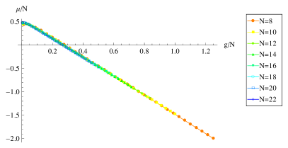
Figure 1: Chemical potential $\mu$ per level versus $g/N$, as computed from Eqs. (11)-(12) for $M=N/2-1$. Here and in the captions of the following figures the pairing coefficient $g$ and the energies are expressed in units of $d$.

III Coupled Richardson Hamiltonians

In this Section we introduce the model studied in the rest of the paper featuring two Richardson models coupled by a tunneling term J62 ; BP82 :

$$H=H_{R}+H_{L}+H_{T},$$ (20)

where $H_{R}$ and $H_{L}$ are the “right” and “left” Richardson Hamiltonian, written in terms of the right and left operators $b_{\alpha,R},b_{\alpha,L}$ (the fermionic operators will be denoted by $c_{\alpha\sigma,R}$ and $c_{\alpha\sigma,L}$ with $\sigma=\uparrow,\downarrow$). We consider the simpler setting in which the two models have the same value of the coupling $g$ and the same energy levels $\varepsilon_{\alpha}$:

$$H_{s}=2\sum_{\alpha=1}^{N}\varepsilon_{\alpha}b^{\dagger}_{\alpha,s}b_{\alpha,s}-2g\sum_{\alpha,\beta=1}^{N}b^{\dagger}_{\alpha,s}b_{\beta,s}\qquad\quad(s=L,\;R),$$ (21)

with the $\varepsilon_{\alpha}$’s equally spaced and given by (2). The number of levels is taken to be equal to $N$ both for the left and the right systems. The total number of pairs in the system is denoted by $M_{T}$ - we will also denote by $M_{L}$ and $M_{R}$ the operators of the number of pairs in the left and right system: $M_{s}=\sum_{\alpha=1}^{N}b^{\dagger}_{\alpha,s}b_{\alpha,s}$ (with $s=L,R$).

We write the tunneling term describing the hopping of a single fermion from one system to the other in the form

$$H_{T}=-\eta\sum_{\sigma=\uparrow,\downarrow}\sum_{\alpha,\beta=1}^{N}\left(c^{\dagger}_{\alpha\sigma,L}c_{\beta\sigma,R}+h.c.\right)$$ (22)

(with $\eta$ having the dimension of an energy). Following the usual approach initially introduced by Josephson J62 , using second-order perturbation theory one can derive an effective Hamiltonian for small values of $\lambda$ (corresponding to the regime of weakly coupled Richardson Hamiltonians): it turns out the this effective Hamiltonian can be written only in terms of the pair operators GSD04 , greatly simplifying the study of the dynamics.

Since the uncoupled Hamiltonians (21) contain only interactions among pairs, the eigenstates of (1) can be classified in terms of their seniority $\nu$, i.e., the number of the unpaired electrons. The second order effective tunneling term can be written as:

$$H^{(2)}=-\sum_{\nu}\sum_{\sigma=\uparrow,\downarrow}\sum_{\alpha,\beta=1}^{N}H_{T}\frac{\left|\alpha_{L}\beta_{R}\sigma;\nu\right\rangle\left\langle\alpha_{L}\beta_{R}\sigma;\nu\right|}{E_{\alpha_{L}\beta_{R}\nu}}H_{T},$$ (23)

in which the sum runs over all the possible intermediate states that can be reached from a $\nu$-seniority couple of states $\left|N/2+\nu\right\rangle_{L}\otimes\left|N/2+\nu\right\rangle_{R}$, by removing an electron of spin $\sigma$ from the level $\beta_{R}$ of the right grain and adding it on the level $\alpha_{L}$ on the left grain (or viceversa). In (23) the quantity $E_{\alpha_{L}\beta_{R}\nu}$ is the corresponding excitation energy relative to the initial state.

Following GSD04 , it is possible to limit the space of states on which the intermediate sum runs over to the lowest energy ones, when acting with (23) on the lowest-energy states of the two uncoupled systems in which all fermions are bound into Cooper pairs. In facts, the energy $E_{\alpha_{L}\beta_{R}\nu}$ includes the energy needed to break a pair and the effect of the blocking of the states on the collective excitations on both subsystems.

Across the whole BCS-BEC crossover, the breaking of a pair associated with the tunneling of a single electron is energetically depressed: processes like the ones depicted in Figure 2(a)-(b) are suppressed by a factor $1/\operatorname{\Delta_{BCS}}$ in the dynamics, since they involve both the breaking of a pair, with an energy cost equal to the BCS gap $\operatorname{\Delta_{BCS}}$ and the blocking of a level, which affects all the levels and has therefore an energy cost roughly proportional to $N$. At second order in the fermion tunneling, it is more convenient to reach a final state in which only Cooper pairs are present J62 . Moreover, single-fermion tunneling does not produce a current in the absence of an applied driving force, so they will not affect the current. This is true in particular for processes like the one in Figure 2(c), which reproduces the initial state and can be included in a redefinition of the energies of the unperturbed system. We are therefore led to consider as dominant the coherent pair tunneling, which involves both the electrons of a Cooper pair and can be directly written in terms of the bosonic operators $b^{\dagger}_{\alpha,L},b_{\beta,R}$ or $b_{\alpha,L}b^{\dagger}_{\beta,R}$, as in Figure 2(d). Assuming the two systems to have a definite relative phase (as it will be checked and discussed in Section IV), the coherent tunneling involves a phase shift on the state in which it takes place and a corresponding variation of the relative number of fermions $\delta N_{f}=\pm 2$ [see Figure 2(d)].

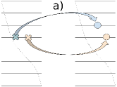
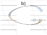
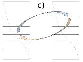
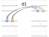
Figure 2: Second-order processes associated to the Hamiltonian (23).

We therefore focus on coherent pair tunneling, for which the effective Hamiltonian is GSD04 ; J62

$$H^{(2)}\approx-\lambda\operatorname{\Delta_{BCS}}\sum_{\alpha,\beta}\frac{b^{\dagger}_{\alpha,L}b_{\beta,R}+b_{\alpha,L}b^{\dagger}_{\beta,R}}{E_{\alpha}+E_{\beta}},$$ (24)

where $E_{\alpha}=\sqrt{\xi_{\alpha}^{2}+\Delta_{BCS}^{2}}$, $\xi_{\alpha}=\varepsilon_{\alpha}-\mu$ and $\lambda=2\eta^{2}/\operatorname{\Delta_{BCS}}$. As can be seen in Eq. (24), we decided to scale the tunneling coefficient with $\operatorname{\Delta_{BCS}}$ since this is the relevant scale throughout the crossover and it is a finite quantity in the thermodynamic limit; furthermore, the form (24) ensures that the tunneling acts as a perturbation also on the BCS side and for small values of $g$.

The form (24) is particularly relevant since it formalizes the fact that preparing the system in its ground state and adding a weak fermionic tunneling term to the uncoupled Richardson Hamiltonians does not destroy the Cooper pairs picture: this provides a major simplification in the problem, allowing for to study the Josephson problem only in terms of hardcore bosons since the subspaces with different seniority will not be accessed neither by the “single-site” dynamics of the uncoupled Richardson systems, nor by the coupling between different sites (see a discussion on the single-fermion tunneling effects at the end of Section IV).

The ground-state state of Hamiltonian $H=H_{L}+H_{R}+H^{(2)}$ was studied in GSD04 and the behavior of the Josephson energy investigated as a function of the level spacing. Integrable versions of coupled pairing Hamiltonians was proposed and studied in ALO01 ; LZMG02 ; GFLZ02 ; LEDPI06 , while an analysis of the spectrum of two weakly coupled Richardson Hamiltonians with $H_{T}\propto\sum_{\alpha,\beta}\left(b^{\dagger}_{\alpha,L}b_{\beta,R}+b_{\alpha,L}b^{\dagger}_{\beta,R}\right)$ was presented in GSD04 ; KNA11 .

In the following we consider the Hamiltonian $H=H_{L}+H_{R}+H^{(2)}$, with $H^{(2)}$ given by (24) and we investigate the properties of its spectrum and the dynamics starting from an state at time $t=0$ having an initial relative phase difference and/or an initial population imbalance: we are interested to ascertain for what values of $N$ a relative phase difference $\delta\phi$ is well defined, and to study the dynamics in terms of the time evolution of $\delta\phi(t)$ and $\delta M(t)$, where $\delta M$ is the difference between the number of pairs of the two systems defined by Eq.(31). Note that, in general, the gap and the chemical potential appearing in (24) will be functions of time as well. However, for the sake of simplicity, we will consider them as constant, which in the present case stands as an approximation valid for small fractional population imbalance.

The initial state is prepared in the following way (see more details in Section IV): the uncoupled system ($\lambda=0$) is initially in the ground state, characterized by a definite occupation number on the left and on the right parts - then, at time $t=0$, the coupling $\lambda\ll d$ is turned on and the quantum dynamics is studied.

Integrability plays an important role both in the study of spectrum and dynamics: it gives the exact eigenstates of the two uncoupled systems and, most importantly, the exact hopping matrix elements. It also provides an efficient truncation mechanism to select the most important eigenstates in the dynamics: as we discuss in the following, one can avoid to diagonalize the Hamiltonian written on a basis of the full Hilbert space of the coupled problem and instead limit its size by restricting only to a subset of states.

Operatively, we start from the basis of the exact eigenstates of the two uncoupled models, with $\lambda=0$, with the number of pairs on the left ($M_{L}$) and on the right ($M_{L}$) separately conserved. Once fixed the total number $M_{T}$ of pairs, the factorized basis $\mathcal{S}_{M_{T}}$ is split into subsectors, each of them characterized by the occupation number of the left model $M_{L}$ and that of the right one $M_{R}$, such that $M_{L}+M_{R}=M_{T}$. Denoting by $S_{M}$ a basis of eigenstates of (3) for the subspace with given number $M$ of pairs, the fixed-number subspaces are spanned by

$$\mathcal{S}_{M_{L},M_{R}}=\left\{\Phi_{L}^{(M_{L})}\otimes\Phi_{R}^{(M_{R})}|\Phi_{L}^{(M_{L})}\in S_{M_{L}}\,,\;\Phi_{R}^{(M_{R})}\in S_{M_{R}}\right\},$$ (25)

so that the factorized basis is

$$\mathcal{S}_{M_{T}}=\bigcup_{M=\max(0,2N-M_{T})}^{\min(N,M_{T})}\mathcal{S}_{M,M_{T}-M}.$$ (26)

It is possible to show that many states in $S_{M}$ are effectively not involved in the dynamics and consequently reduce the space of quantum states to a computationally manageable size: to see this, let first consider the limits $g\to 0$ and $g\to\infty$. In the non-interacting case, the single-level occupation numbers are good quantum numbers for the system: it follows that all the excitations above the Fermi sea ground state induced by the coupling, in the regime in which the tunneling coupling is small ($\lambda/d\ll 1$), are the states in which one particle is missing from the Fermi sea or one particle is added above it. These are a subset of the “particle–hole” states, obtained from exciting one pair from below to above the Fermi level, which are instead there at second order.

In the opposite limit $g\to\infty$, it is useful to rewrite (3) in terms of spins, obtaining the spin Hamiltonian (5): in the strong coupling limit $g\to\infty$, the Hamiltonian (5) reads YBA03

$$H\approx-2g\left(\vec{S}\cdot\vec{S}-\left(S^{z}\right)^{2}-S^{z}\right)$$ (27)

(where $\vec{S}=\sum_{\alpha}\vec{S}_{\alpha}$) and it conserves the total spin of the state and its $z$-projection. Numerical solutions of the Richardson equations show that the rapidities can either diverge proportionally to $g$ or remain finite, with real part which lies “trapped” between two energy levels. In the strong coupling limit, the tunneling Hamiltonian. Consequently, the states group into highly degenerate total spin subspaces YBA03 . In the strong coupling limit, the tunneling Hamiltonian (23) simplifies as well: the BCS gap diverges linearly with $g$ and all the pairs of levels in (24) factorize a common term, yielding

$$H^{(2)}\approx-\frac{\lambda\operatorname{\Delta_{BCS}}}{\sqrt{\Delta_{BCS}^{2}+\mu^{2}}}S^{+}_{tot,L}S^{-}_{tot,R}+h.c.$$ (28)

(where $\vec{S}_{L}=\sum_{\alpha}\vec{S}_{\alpha,L}$ and where $\vec{S}_{R}=\sum_{\alpha}\vec{S}_{\alpha,R}$). The ground state is the unique state in which all the rapidities diverge in the strong coupling limit and it is the one with highest (total) spin. The relation between the number $r$ of diverging roots at strong coupling and the eigenvalues of the spin Hamiltonian (27) is $r=s-s^{z}$ YBA03 , being $s(s+1)$ and $s^{z}$ the total spin projection along the $z$ axis. One then sees that it is sufficient to restrict the single-site Hilbert space to the root configurations with one less (or one more) rapidity and the same number of rapidities which diverges at large $g$, i.e., again the ground state of the new sector: therefore, no new state is needed. Although the previous arguments are valid in the two limiting regimes $g\to 0$ and $g\to\infty$, we numerically compared the results with exact diagonalization (for $N=6$) or the effect of adding more total spin subspaces to the dynamics (for $N=8$). In all the tests we performed, results in excellent agreement were found.

Algorithms for connecting the number of roots that eventually diverge to the initial state configurations have been given in FCC08 ; SRD03 : the included states are exemplified in Figure 3 and consist of the evolution in $g$ of all the configurations in which, in the weak coupling limit, one particle is excited from the Fermi sea to right above its surface or from the Fermi energy to one more energetic state.

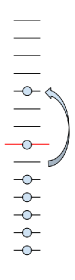
Figure 3: Particle-hole states.

The algorithm used for solving the Richardson equations numerically is based on the one described in BDS11 . To obtain eigenstates at a given $g$, one starts from $g=0$, where the rapidities that solve the Richardson equations are known within good approximation. It is therefore possible to solve numerically (9) for some values of $g$ around zero: the coefficients of the polynomial having these rapidities as roots are computed. One then extrapolates these coefficients to a new value of the pairing, in steps $\delta g\simeq 0.01d$, and compute the roots of the extrapolated polynomial, using them as a starting guess for the numerical solution of the Richardson equations. The procedure is iterated up to the desired value of $g$ BDS11 (see more details in B12 ). This algorithm allows to solve every configuration for sizes $N\leq 10$, which we used in this paper. A numerical procedure for dealing with general Gaudin models has been presented in FEASG11 . Once that the factorized basis has been determined, we write the tunneling term by using Eq. (16), and diagonalize the resulting Hamiltonian.

III.1 Properties of the spectrum

In Figure 4 we plot the energy spectrum for two coupled Richardson models as a function of the tunneling parameter $\lambda$ for three different values of $g$. It is seen that the effect of a weak tunneling on the spectrum depends essentially on the coupling among fermions: one can clearly identify a regime of nearly non-interacting particles, in which the quasi-degeneracy of the levels is given by the number of ways of promoting one or more particles in an excited level to obtain a given energy (degeneracy is a consequence of the choice of equally-spaced levels). In this regime, the perturbation splits the levels of one band as far as the band spacing, hence giving rise to a spectrum in which the original degeneracies are not seen any more.

On the other hand, in the strong coupling regime states group into eigenstates of the total angular momentum, as seen from the spin representation (27). Since the distance among the energies of these subspaces is of order $g$, in this regime, even a tunneling term of several times the gap cannot mix the different subspaces among them.

In the crossover region, the strong coupling subspaces are already quite defined, but not far one from the other. It follows that a sufficiently strong perturbation can still hybridize them. To better illustrate this point, we may evaluate how much the levels are shifted by turning on $\lambda$: however, the absolute value of the shift should be compared with the level spacing in a situation where levels are well-distinguishable (intermediate couplings) and the band spacing in the presence of strong degeneration ($g\to 0$ or $g\to\infty$).

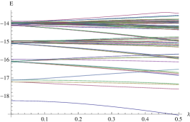
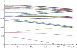
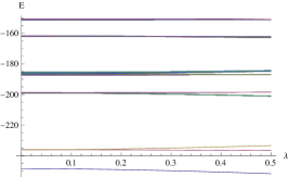
Figure 4: Energy spectrum vs. $\lambda$ for $N=8$ and $M_{T}=8$, with $g=0.1$ (left), $g=1.2$ (center), $g=6.2$ (right) - for simplicity, thereafter also $\lambda$ is expressed in units of $d$.

A convenient way to proceed is to divide the all spectrum in a certain number of interval (let $N_{bin}$ this number) and count how many levels lie in each interval: we define the quantity

$$\chi_{m}\equiv(\#\;levels\;in\;the\;m^{th}\;interval)(\lambda)-(\#\;levels\;in\;the\;m^{th}\;interval)(\lambda=0).$$ (29)

The average of this quantity with respect to the interval index $m$ is obviously zero. The relevant quantity is instead its standard deviation $\sigma_{\chi}$: the result is plotted in Figure 5, left part. The quantity $\sigma_{\chi}$ has a maximum around $g/d\sim 1$, corresponding to the point in which the degeneracies of the noninteracting picture are already destroyed, while the energy bands of the strong coupling regime are not evident yet. This result is of course related to the occurrence of a crossover between weakly attracting fermions and tightly bound pairs: for the uncoupled systems, from the point of view of the energy spectrum the crossover reflects itself on the creation of energy bands out of the pair levels, which are more and more separated by increasing $g$. This is also seen at the level of the coupled spectrum, The doublet structure characterizing coupled noninteracting systems is melted into an highly-degenerate band structure.

In the right part of Figure 5, we plot the energy difference between the first excited state and the ground state in a system with an odd number of particles as a function of $g$. It turns out that, as long as the gap opens more and more, the energy difference between the components of the level doublet reaches a maximum splitting.

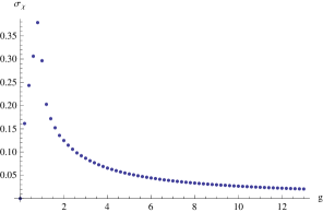
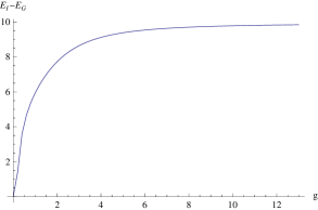
Figure 5: Left: standard deviation $\sigma_{\chi}$ vs. $g$ associated with the level structure, given by ($N_{bin}=100$, $\lambda=0.05$, $N=8$, $M_{T}=6$). Right: energy difference between the first excited state and the ground state as a function of $g$ for the same values of the parameters.

IV Emergence of a definite relative phase

In this Section we explain what initial states have been considered and we discuss how a definite relative phase emerges for small number of particles and our algorithm for obtaining it from numerical data.

The initial state $\left|\Psi(t=0)\right\rangle$ is prepared in a linear combination of ground states of the uncoupled systems having a different number of pairs and therefore a population imbalance: this state is evolved in time with the dynamics generated by (20), with $\lambda\neq 0$ in the tunneling term. More precisely, at $t=0$ the system is generically in a linear superposition of two states with a given number of pairs (we choose $M_{0}$ in a system and $M_{0}-D$ in the other): the total number of pairs is conserved during the time evolution and is $M_{T}=2M_{0}-D$. Denoting by $\left|\Phi_{M}^{(L,R)}\right\rangle$ the lowest-energy state with $M$ pairs of either the left or the right system, we prepare the system in the state

$$\left|\Psi(t=0)\right\rangle=\frac{1}{\sqrt{1+\xi^{2}}}\left(\left|\Phi_{M_{0}}^{(L)}\right\rangle\otimes\left|\Phi_{M_{0}-D}^{(R)}\right\rangle+e^{i\phi_{0}}\xi\left|\Phi_{M_{0}-D}^{(L)}\right\rangle\otimes\left|\Phi_{M_{0}}^{(R)}\right\rangle\right):$$ (30)

given the limitation on the total number of pairs ($M_{T}\leq 10$), we will most consider $D=1$, therefore creating as initial state by a linear superposition of $M_{0}$ in a system and $M_{0}-1$ in the other, and $D=2$ (typically we choose $M_{0}=N/2$ or $M_{0}=N/2\pm 1$).

Given $\left|\Psi(t)\right\rangle$, one can compute the pair population imbalance as

$$\delta M(t)\equiv\left\langle\Psi(t)\left|M_{L}-M_{R}\right|\Psi(t)\right\rangle=\left\langle\Psi(t)\left|\sum_{\alpha}\left(b^{\dagger}_{\alpha,L}b_{\alpha,L}-b^{\dagger}_{\alpha,R}b_{\alpha,R}\right)\right|\Psi(t)\right\rangle$$ (31)

(the population imbalance $\delta N_{f}$ is just $\delta N_{f}=2\delta M$). Notice that with $\xi=0$ it is $\left\langle\Psi(t=0)\left|M_{L}\right|\Psi(t=0)\right\rangle=M_{0}$.

According to the notation of SFGS97 , we will denote by $z(t)$ the fractional population imbalance:

$$z(t)=\frac{\delta M(t)}{M_{T}}.$$ (32)

Using the state (30) one simply obtains

$$\delta M(t=0)=D\,\frac{1-\xi^{2}}{1+\xi^{2}}:$$

therefore varying the parameter $\xi$ one can choose different initial population imbalances (with $\left|\delta M(t=0)\right|\leq D)$. The dynamics is then studied turning on a small perturbation ($\lambda/d=0.01-0.1$ in our runs) and compute the time evolution of the state after exact diagonalization the Hamiltonian. The main limitation of this protocol arises from the consume of RAM by diagonalization subroutines: by limiting subspaces appropriately, as discussed in Section III, one can study systems up to $N=10$ levels (both on left and right systems).

An important issue we want to address in this Section, arising from the fact that we can treat the exact quantum dynamics of the coupled model only for a limited number of pairs, is whether a definite relative phase emerges at small sizes. In the presence of the tunneling term (23), eigenstates will in principle be written as a combination of many of the factorized states of the two uncoupled Hamiltonian. Nevertheless, as we will see, when the initial population imbalance is small, the number of involved states is rather small. Moreover, even for higher particle imbalance, when the tunneling is weak and the pairing strength is strong enough, the Hilbert space of each system organizes in subspaces, labeled by eigenvalues of the total spin (see Section II). It follows that in most cases, even if the exact states involved are many, the corresponding energy eigenvalues are not very different, therefore the time evolution takes place with nearly definite phase.

Note that in our canonical setting the expectation value $\left\langle\Psi(t)\right|b_{\alpha,L/R}\left|\Psi(t)\right\rangle$ is always vanishing, since the $b$’s operators does not conserve the number of particles. However, we can define time-dependent phase differences between one level in a system and a level in the other system systems by the use of the formalism of Section II evaluating the dynamical two-point functions (for the uncoupled systems, dynamical two-point correlations have been studied ZLGM03 ; FCC10 ).

From the correlation function $\left\langle\Psi(t)\right|b^{\dagger}_{\alpha,L}b_{\beta,R}\left|\Psi(t)\right\rangle$ one can extract how much the phases of two distinct levels differ at a given time. In particular, we considered two different procedures for the choice of the levels, which can be tested one against the other, and define:

$$w_{\alpha}(t)=\left\langle\Psi(t)\right|b^{\dagger}_{\alpha,L}b_{\alpha,R}\left|\Psi(t)\right\rangle$$ (33)

and

$$z_{\alpha}(t)\equiv\left\langle\Psi(t)\right|b^{\dagger}_{\alpha,L}b_{N/2,R}\left|\Psi(t)\right\rangle.$$ (34)

In (34) the subscript refers to the level on the left system and a reference state is taken on the right system (arbitrarily chosen to be the level $N/2$); conversely, in (33), the level is chosen to be the same on both systems. We define a relative phase between levels as

$$w_{\alpha}(t)\equiv\left|w_{\alpha}(t)\right|e^{i\delta\phi_{w}(t;\alpha)}$$ (35)

and

$$z_{\alpha}(t)\equiv\left|z_{\alpha}(t)\right|e^{i\delta\phi_{z}(t;\alpha)}.$$ (36)

The functions $\delta\phi_{w}(t;\alpha)$ and $\delta\phi_{z}(t;\alpha)$ are functions of both time and level index. It is then necessary to verify whether the levels have small phase difference: to do this, we define the level average

$$\delta\phi_{w,z}(t)=\frac{1}{N}\sum_{\alpha=1}^{N}\delta\phi_{w,z}(t;\alpha)$$ (37)

and their standard deviation $\sigma_{w,z}(t)$ [with $\sigma_{w,z}^{2}(t)=(1/N)\sum_{\alpha=1}^{N}(\delta\phi_{w,z}(t;\alpha)-\delta\phi_{w,z}(t))^{2}$]. The time evolution of the mean values $\delta\phi_{w,z}(t)$ is reported in Figure 6: one sees that already for $M_{T}=8$, one has relatively small values of $g$ where the two definitions of the relative phase are in good agreement for most of the times. The two definitions $\delta\phi_{w}(t)$ and $\delta\phi_{z}(t)$ are expected to agree only when the two systems show coherent behavior, and the phase difference between them is, within a good approximation, given by the phase difference between any two levels chosen. We checked that choices other than (33)-(34) give practically the same results when a relative phase is well defined.

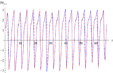
Figure 6: Phase differences $\delta\phi_{w}(t)$ (solid blue line) and $\delta\phi_{z}(t)$ (dotted red line) vs. $t$ for the coupled systems with $N=8$ levels each, total number of pairs $M_{T}=8$, pairing strength $g=0.6$, tunneling parameter $\lambda=0.1$, $D=2$ (corresponding to $M_{0}=5$) and initial imbalance $z(t=0)=0.25$. Time here and in the following figures is in units of $\hbar/d$.

In order to have a definite relative phase one has to check that the average values $\delta\phi_{w,z}(t)$ should be (possibly for most of the considered times) much larger than their standard deviations $\sigma_{w,z}(t)$: as shown in Figures 7 and 8 (done respectively for $g=0.2d$ and $g=0.6d$) this condition is rather well verified also for a number of pairs $M_{T}=8$. One also sees that for $g=0.2d$ the agreement is less good, as expected also from the fact that - as discussed in Section II - the uncoupled systems have significant deviations from the large-$N$ limit. We also observed for the considered values of $g$ a significant degradation of the relative phase for even smaller total number of pairs, e.g. as low as $M_{T}=4$.

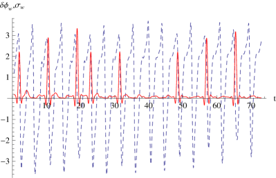
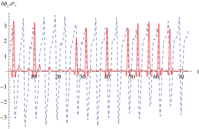
Figure 7: Phase difference means $\delta\phi_{w,z}(t)$ (dashed blue lines) and standard deviations $\sigma_{w,z}$ (red solid lines), as determined from the correlation functions $w$ (left) and $z$ (right), for two coupled grains with the same parameters as in the previous Figure.

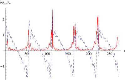
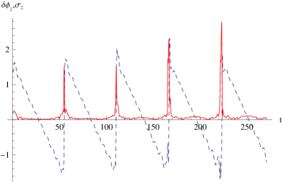
Figure 8: Same quantities as in Figure 7 with $g=0.2$ (other parameters unchanged).

Information about the phase difference averages and their standard deviations at every given time is useful, but we can complement it with their averages in time: to this purpose, we consider the mean of the standard deviation presented above over sufficiently long times (several periods)

$$C_{w,z}^{\delta\phi}=\frac{1}{t_{max}}\int_{0}^{t_{max}}\sigma_{w,z}(t^{\prime})dt^{\prime}.$$

To establish a comparison, we need to evaluate also the mean phase difference among the condensates. This is an oscillating quantity, having vanishing average on time: we then compute the average of its square:

$$S_{z,w}^{\phi}=\sqrt{\frac{1}{t_{max}}\int_{0}^{t_{max}}\delta\phi_{z,w}^{2}(t^{\prime})dt^{\prime}}.$$

In Figure 9 we plot $C^{\delta\phi}$ and $S^{\delta\phi}$ with both the definitions (33)-(34). One sees already for $g\gtrsim 0.3d$ a very good agreement $C^{\delta\phi}_{w}$ and $C^{\delta\phi}_{z}$, and both significantly larger than the time averages $S^{\delta\phi}_{w,z}$. For this reason we are going to denote as $\delta\phi$ the relative phase difference, omitting the indexes $w,z$. One also sees that for small $g$ the relative phase is not defined, as expected, since the relative phase is comparable with its variance.

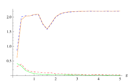
Figure 9: $C^{\delta\phi}_{w}$ (lower dashed line), $S^{\delta\phi}_{w}$ (upper dashed line) and $C^{\delta\phi}_{z}$ (lower solid line), $S^{\delta\phi}_{z}$ (upper solid line) vs. $g$. Parameters are as in Figures 6-8: $N=8$, $M_{T}=8$, $\lambda=0.1$, $D=2$ (moreover, $t_{max}=1000$).

As a function of the pairing parameter $g$, from Figure 9 one sees that the higher is the value of $g$, the more the system shows a definite relative phase. We also observed that the smaller is the tunneling parameter, the sooner (in $g$) a definite phase is established. Similarly, a small initial imbalance allows for a definite phase to emerge for relatively small values of $g$, while - for the considered values of $N$ - stronger pairing is necessary if states with larger initial imbalances are selected. This is due to the fact that the initial state is projected on few states in the lowest part of the spectrum when the initial population difference is small. Conversely, larger population imbalances at $t=0$ are projected to many states in the middle of the spectrum, each having its own energy.

We pause here to comment about fermion tunneling: as a matter of fact, the original tunneling Hamiltonian (22) is written in terms of fermionic operators, while the result that the phase coherent behavior is established with relatively small pairing and/or total number of pairs is obtained with the bosonic approximation (24), acting on the restricted subspace of blocked levels. Since at small $g$ pair-breaking excitations may play an important role, a natural question to ask is whether the presence of fermionic degrees of freedom, aside of bosonic pairs, may spoil the phase-coherent behavior of the systems for sufficiently large pairing. The issue can be rephrased into the question of whether the initial state, during the evolution generated by the coupled Hamiltonian, containing a fermionic tunneling term, may give rise to a huge number of states in which two or more electrons are not paired, evolving incoherently with respect to the states in which only pairs appear.

These states have to be written as linear combinations of the factorized states of the two uncoupled Hamiltonians. On each site, the energy of such states can be exactly computed for any value of $g$. In order to have an estimation of a lowest bound for the energy, we can consider a state in which the most energetic pair is broken and one electron is promoted into the next level, which reduces the number of pairs by $1$ and the number of unblocked levels by $2$, as seen in Section II. The energy of the lowest pair-breaking excitation has been considered in YBA03 and it reads:

$$E_{pair}\simeq\frac{\varepsilon_{M}+\varepsilon_{M+1}}{2}-g(M-1)((N-2)-(M-1)+1)$$ (38)

The bare energies in the first term of (38) do not depend on $g$, unlike the ground state energy, all the pair-conserving excitations and the second term in the previous equation. It follows that, by taking the pairing strength sufficiently high, all pair-breaking excitations can be made to lay at arbitrary energy above the ground state and are therefore suppressed with respect to pair-conserving excitations.

Checking explicitly that the insertion of states with unpaired electrons does not spoil the phase relation requires much larger computational effort, in that the Hilbert space should be enlarged to the $\binom{N}{m}\binom{N-m}{M}$ configurations in which the $m$ electrons can “block” part of the $N$ levels, with fixed number $M$ of pairs. We can therefore qualitatively rely on the standard argument based on the presence of a gap preventing single-fermion tunneling: note that this should already hold for values of $g\gtrsim 0.25$, as previously discussed.

We also mention that, even if the phase is quite well defined, residual fluctuations can still be observed, in such a way that the widest, slowest oscillations are superimposed with faster and narrower ones. We find convenient to isolate the former ones by computing time averages on intervals much smaller than the period of the largest oscillations: this allows to better understand the structure of the dynamical diagrams discussed in the next Section. An example of the procedure is provided in Figure 10.

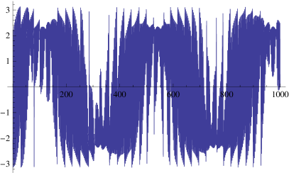
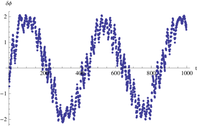
Figure 10: Left: phase difference, as a function of time, for $N=8$, $M_{T}=6$, $\delta M_{0}=2$, $g=5$, $\lambda=0.05$. Right: averaging over short times $t_{av}$ (here, $t_{av}=6$) to remove fluctuations.

V Phase portrait and current-phase characteristics

In this Section we first draw the population-phase dynamical portrait $z(t)$-$\delta\phi(t)$ as it has been done for bosonic Josephson junctions SFGS97 ; RSFS99 and we determine the current-phase characteristics, which is a typical tool used to characterize the behavior of a Josephson junction L79 ; BP82 . From the solution for the quantum dynamics one can extract the dominant period of the population oscillations and determine the Josephson frequency. We also comment on the determination of a two-state model giving a good description of the dynamics and of the current-phase characteristics for the considered initial conditions. We observe that most of our simulations are done for the initial state (30) with $D=1$ build by a linear combination of a state with $M_{0}=N/2$ pairs on a system and $M_{0}=N/2-1$: this state has a maximum value for $\left|\delta M(t=0)\right|$ equal to $1$. For this initial state the relative phase difference $\delta\phi$ is well defined for a total number of pairs $\gtrsim 6$ and for $g\gtrsim 0.3$ (see Figure 9), where the expectation values for the correlation functions are already rather similar to the large-$N$ BCS findings FCC08 : we can then explore the crossover region (which is around $g/d\sim 0.25N$). In the final part of the Section we consider $D=2$ and initial imbalance $\delta M(t=0)=2$: the phase turns yet to be again rather well defined (but a larger values of $g$), but we cannot practically explore larger initial imbalances (i.e., larger values of $D$) since with our maximum value of pairs $M_{T}\sim 10$ the relative phase is well defined only for very large values of $g$ (well beyond the crossover point).

In Figure 11 we plot the number-phase portrait where we plot as a function of time both $\delta\phi(t)$ and $\delta M(t)$ for different values of $\delta M(t=0)$. It is also possible to study the diagram while varying the initial phase in the initial state (30), as shown in Figure 12.

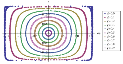
Figure 11: Dynamical phase-portrait $z$-$\delta\phi$ for different values of the parameter $\xi$ in the BCS regime, with $N=8$, $M_{T}=7$, $D=1$, $g=0.57$, $\lambda=0.05$. The chosen values of $\xi$ are $\xi=0.1,0.2,0.3,0.4,0.5,0.6,0.7,0.8,0.9$ corresponding respectively to $\delta M(t=0)=0.98,0.92,0.83,0.72,0.60,0.47,0.34,0.22,0.10$.

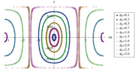
Figure 12: Phase portrait for different initial phases in the BEC regime ($N=8$, $M_{T}=7$, $D=1$, $\delta M(t=0)=1$, $g=9.7$, $\lambda=0.05$).

One sees from Figures 11-12 that even for a small total number of pairs ($M_{T}=7$) the phase diagram in the plane $\delta\phi-z$ shows a remarkable agreement with a "pendulum" law of motion in the small oscillations regime when the initial imbalance is small. Furthermore, as the initial displacement or phase difference becomes larger, significant corrections are seen.

A way to understand such results is to introduce a two-state model BP82 ; FLS65 : computing the overlaps of the initial state (30) having $D=1$ and $|\delta M(t=0)|\leq 1$ with the many-body eigenfunctions of the full Hamiltonian (with $\lambda$ small), one sees that the largest overlaps are with the ground and the first excited states. Given this one expects that the dynamics is well explained by a simple linear two-mode model involving such two states. The dynamical equations of the Feynman two-state model are reviewed in Appendix A: for the linear two-state model here considered the phase difference $\delta\phi$ does not overcome the value $\pi/2$, i.e., if $\left|\phi(t=0)\right|<\pi/2$, then $\left|\phi(t)\right|<\pi/2$. As seen in Figures 11-12, this property is clearly observed in the numerical results (we also checked it with exact diagonalization). The property is typical of the linear two-mode model and it is connected with the fact that the main contributions to the time-dependent wavefunction arise from the first two lowest-lying states of the interacting system with equal weights.

We now focus on the pair current between the models: we define the current $I$ as the time derivative of the occupation number of the left subsystem

$$I(t)\equiv\frac{d}{dt}\left\langle\Psi(t)\left|M_{L}\right|\Psi(t)\right\rangle=\frac{d}{dt}\left\langle\Psi(t)\left|\sum_{\alpha}b^{\dagger}_{\alpha,L}b_{\alpha,L}\right|\Psi(t)\right\rangle.$$ (39)

From Eq. (39) one finds

$$\hbar I(t)=i\left[H,M_{L}\right]=i\left[H^{(2)},M_{L}\right]=i\sum_{\alpha,\beta}\frac{b_{\alpha,L}b_{\beta,R}^{\dagger}-b_{\alpha,L}^{\dagger}b_{\beta,R}}{E_{\alpha}+E_{\beta}}.$$ (40)

As discussed in the Appendix A, for the linear two-state model the current is proportional to the tangent of the phase difference: $I\propto\tan{\delta\phi}$ [see Eq. (54)]. The current-phase characteristic can be therefore written as

$$I(\delta\phi)=I_{c}(g,\lambda)\tan{\delta\phi}$$ (41)

and the critical current $I_{c}$ can be fitted from numerical data. An example is given in the left part of Figure 13. We find that the critical current has a maximum around a finite value of $g$, as shown in the right part of Figure 13: for the considered values of $N$ the maximum is at $g\simeq 1$, close to the unitary regime. $I_{c}$ can be fitted in the form

$$I_{c}(g,\lambda)=I_{0}\lambda\frac{e^{-c/g^{2}}}{g}:$$ (42)

$I_{0}$ depends mostly on $N$. Notice that the relation (42) has a maximum at $g^{*}=\sqrt{2c}$. For the parameters of Figure 13 we find $c\simeq 0.27$, nearly independent on $\lambda$.

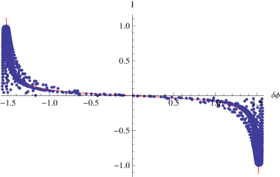
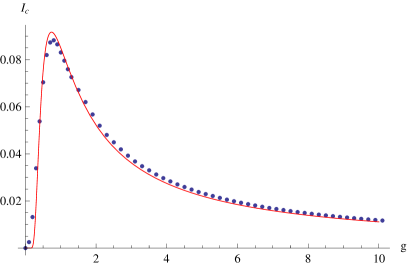
Figure 13: Left: fit for the $I$-$\delta\phi$ characteristics with $g=2.3$, $\lambda=0.05$, $D=1$, $\delta M(t=0)=1$, $N=8$, $M_{T}=7$ - blue circles are numerical points obtained from the quantum dynamics, and the red line is the fit according Eq. (41). Right: critical current fit - the blue circles are numerical results, while the red line is Eq. (42) with $c\simeq 0.27$.

We stress that the fit needed to identify the critical current is done using the linear two–mode model: the validity of the fit relies on the fact the two lowest levels are the ones mainly involved in the dynamics, which is the case for small imbalances ($D=1$). Deviations are observed for larger values of $D$, as we are going to discuss.

It is an interesting issue to explore what happens when more levels, inserted in a band structure as the one described in Section III.1, participate the dynamics: with $D=2$ and $\delta M(t=0)=2$ the phase diagram shows a typical ellipsoid form. An example of number-phase portrait is given in Figure 14. We see that the phase range depends only on the interaction, while the amplitude of the population oscillations depends on the initial relative phase given to the system through (30).

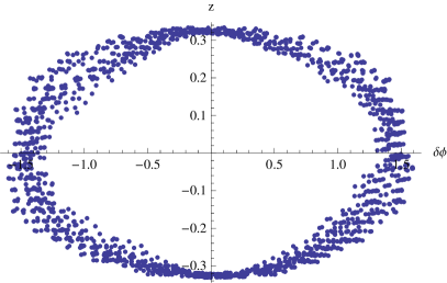
Figure 14: Number-phase diagram for $N=8$, $D=2$, $\delta M(t=0)=2$, $M_{T}=6$, $\lambda=0.05$ and $g=0.4$.

The numerical study of the current phase characteristics reveals that for $D=2$ the relation (41) does not provide a good way of fitting the critical current: the numerical results are plotted in the left part of Figure 15. We find that a good approximation of the current-phase characteristics is given by

$$I(\delta\phi)=I_{c}(g,\lambda)\sin\frac{\delta\phi}{2}$$ (43)

with $I_{c}$ given by (42) note1 , as it can be seen in the right part of Figure 15. We observe that such a dependence for the current-phase characteristics was found for a weak, point-like barrier in the WKB approximation in the Bogoliubov-de Gennes equation BH91 . Since for large $N$ we expect a dependence $\propto\sin{\delta\phi}$ SPS10 , we attribute the result (43) to the small $N$ considered: further numerical investigations with larger number of levels are needed in order to obtain the current-phase characteristic for intermediate and large $N$ for the coupled Richardson models.

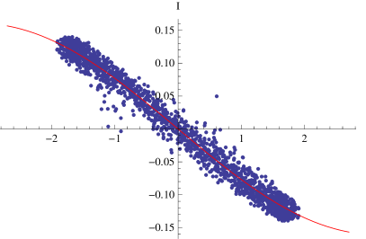
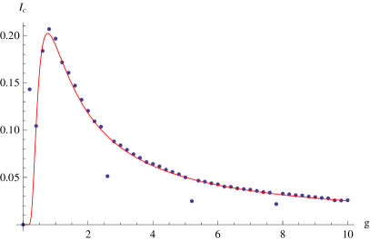
Figure 15: Left: current-phase characteristics for $g=3.8$, $\lambda=0.05$, $D=2$, $\delta M(t=0)=2$, $N=8$, $M_{T}=7$ - blue circles are numerical points obtained from the quantum dynamics, and the red line is the fit according Eq. (43). Right: critical current vs. $g$ - the blue circles are the numerical results, while the red line is Eq. (42).

A check of Eq. (43) and of the data presented in Figure 15 can be obtained by doing the Fourier transform of $\delta M(t)$ with $D=2$: as a function of $g$, to a very good approximation the dominant frequency of $\delta M(t)$ (i.e., the Fourier component with the highest weight) turns out to be proportional to the critical current given by (42).

An important prediction of the nonlinear two-state model is that there is a critical initial imbalance for which self-trapping occurs SFGS97 : given the limitation on the maximum value of $D$, we cannot explore larger initial imbalances. What is observed, instead, is that the amplitude of the fastest oscillations of $\delta M(t)$ is increased and that the period of the slowest ones is decreased more and more, as $1/g$. The time period of both $\delta M(t)$ and $\delta\phi(t)$ become larger and the oscillations exhibited by $\delta\phi(t)$ (as the ones seen in the left part of Figure 10) become as well larger. The scenario is that of a large crossover to a confined regime, in which the occupation oscillations have infinite period at $g$ very large. This may be a finite-$N$ effect, and one could expect that this eventually leads to a transition in the thermodynamic limit.

The initial phase can also be varied with initial imbalance $\delta M(t=0)=2$. It is interesting to note that the for most of the values of $g$, the phase runs: nevertheless, the time evolution of the mean phase locks it around some large-period oscillations. We conclude by observing that similar results are found decreasing the coupling $\lambda$: further investigations to study self-trapping effects at very small values of the coupling are needed. An analysis of larger imbalances and larger $N$ (eventually with very small coupling) is therefore needed to study self-trapping effects, and more in general non-linear effects, through the crossover.

VI Conclusions

We have studied the emergence of a definite relative phase between ultrasmall metallic grains (and in general finite-size systems of attractively interacting fermions) modeled by weakly coupled Richardson models. We have introduced and discussed a way of extracting the relative phase and its variance from the many-body wavefunction, in order to precisely quantify whether a definite relative phase emerges.

We have also related the coherent behavior to the spectrum of the coupled systems and suggested a criterion to characterize the crossover between the BCS and BEC regimes, showing that these regimes are clearly distinguishable by the spectrum of the coupled models.

Moreover, we have performed a numerical analysis of the exact dynamics of the two weakly coupled Richardson Hamiltonians, after a weak tunneling term is turned on. We used a linear superposition of the eigenstates of the two uncoupled systems, with a different number of pairs ($D$ being such difference), as initial states: these states are then evolved according to the full Hamiltonian including the tunneling Hamiltonian, weakly coupling the two systems. We found that a definite relative phase difference emerges even for a small numbers of pairs ($\sim 8-10$). Therefore, the current-phase characteristics could be obtained for values of the bare pairing strength for which the equilibrium properties of the uncoupled models are well approximated by the BCS theory. We showed that, for small initial imbalances ($D=1$), a two-state model gives a reasonably good description of the dynamics and of the current-phase characteristics.

Finally, we have presented the critical current as a function of the pairing parameter, finding that it has a maximum around the unitary regime, even with a number of pairs $\sim 8$. The phase portrait was studied for small initial imbalances ($D\leq 2$).

The requirement of having a definite phase difference among the two systems with a limited total number of pairs ($\leq 10$) prevented us to analyze values of the initial population imbalance ($D>2$): for these large initial imbalances the relative phase is well defined only for very strong pairing interaction, well beyond the unitary limit and deep in the BEC regime. Further numerical investigations are required to consider larger sizes and larger initial imbalances (eventually with very small tunneling couplings), which may generate a definite relative phase across the BCS-BEC crossover: it is expected that a proper finite-size scaling may be crucial to identity non-linear self-trapping effects. We moreover regard as interesting the investigation of the effects on the relative phase of single-fermion tunneling terms: these terms might give a contribution on the BCS side of the crossover and produce a degradation of the relative phase, which should eventually form for larger sizes. Similarly, it would be stimulating to compare (eventually for larger systems) the results obtained from exact dynamics with the ones obtained using time-dependent mean-field approaches.

The rapid growth of the computational cost with the size of the systems represents a limitation on the total number of pairs as well: the Hilbert space could be further reduced in the strong coupling regime, yet not throughout the whole crossover. We conclude that it stands as an open issue, certainly deserving future work, how our findings scale with the size of the system.

Our results can be applied to weakly coupled ultrasmall metallic grains and to cold atom experiments in which traps with few fermions are set at a distance that allows tunneling: the individuation of the relative phase between nearest neighboring sites makes possible in perspective to study Josephson dynamics and self-trapping systems also for larger imbalances, and to check the validity of two- and multi- mode ansatz.

We finally observe that in this paper we focused our attention to weakly coupled Richardson models, discussing the formation of a relative phase and the Josephson dynamics for a class of considered initial conditions. The extension of our method of defining a relative phase to the problem of the formation of a relative phase between general interacting (both integrable and non-integrable) mesoscopic systems could be relevant in a rather broad class of physical systems, including weakly coupled ultracold finite Bose gases, and it is in our opinion an interesting problem, worthwhile of future studies.

Appendix A Dynamical equations for the two-state model

A general description of the tunneling in superfluid/superconducting systems is provided by the Feynman two-state model FLS65 : the macroscopic wavefunctions $\psi_{L}$ and $\psi_{R}$ of the left and right systems obey the equations

$$i\hbar\frac{\partial\psi_{L}}{\partial t}=E_{L}\psi_{L}-K\psi_{R}$$ (44)

$$i\hbar\frac{\partial\psi_{R}}{\partial t}=E_{R}\psi_{R}-K\psi_{L}.$$ (45)

The two-state model also describes also the tunneling of Bose-Einstein condensates in double well potentials SFGS97 : the effect of the interactions between atoms in the wells results in cubic terms of the form $U\left|\psi_{L}\right|^{2}\psi_{L}$ and $U\left|\psi_{R}\right|^{2}\psi_{R}$ added to the right-hand sides of Eqs. (44)-(45). In our case, since the $D=1$ initial state (30) has mostly projections on the ground and first excited many-body states, we limit ourself to Eqs. (44)-(45) (with $U=0$).

Setting $\psi_{s}=\sqrt{M_{s}}e^{i\phi_{s}}$ (with $s=L,R$), the equations for $z\equiv(M_{L}-M_{R})/(M_{L}+M_{R})$ and $\phi\equiv\phi_{R}-\phi_{L}$ reads

$$\hbar\frac{\partial z}{\partial t}=-2K\sqrt{1-z^{2}}\sin\phi,$$ (46)

$$\hbar\frac{\partial\phi}{\partial t}=\frac{2Kz}{\sqrt{1-z^{2}}}\cos\phi$$ (47)

for the symmetric case $E_{L}=E_{R}$.

The system (46)-(47) can be derived from the Hamiltonian

$${\mathcal{H}}=-2K\sqrt{1-z^{2}}\cos{\phi}$$ (48)

in which the time evolution of the conjugated variables $\phi,z$ is found from

$$\hbar\dot{z}=-\frac{\partial{\mathcal{H}}}{\partial\phi}$$ (49)

$$\hbar\dot{\phi}=\frac{\partial{\mathcal{H}}}{\partial z}.$$ (50)

By defining the angular variable $\theta$ such that $z=\sin\theta\,\in\left[-1,1\right]$, one finds from (48)

$$\hbar\dot{\theta}=\mp 2K\sin\phi$$ (51)

$$\hbar\dot{\phi}=2K\tan\theta\cos\phi:$$ (52)

where the $\mp$ sign accounts for the determination of the square root. The time-dependent relative occupation is a function of time only through the relative phase $\phi$. Starting from (51)-(52) and identifying with a prime the derivative with respect to $\phi$, one has

$$\hbar\frac{d\theta}{dt}=\hbar\frac{d\theta}{d\phi}\frac{d\phi}{dt}=\mp 2K\sin\phi,$$

from which

$$\tan\theta\frac{d\theta}{d\phi}=\mp\tan\phi.$$

By integration one obtains

$$\cos\theta=\frac{A_{0}}{\cos\phi},$$ (53)

where the constant $A_{0}=\mp\cos\phi_{0}\cos\theta_{0}$ is fixed by the initial conditions. Defining the current $I$ as $I=\dot{M}_{L}$ one has $I=M_{T}\dot{z}/2$ where $M_{T}=M_{L}+M_{R}$ is the total number of particles (pairs, in our case). Using (46) one has

$$I(\phi)=\frac{M_{T}}{2}\dot{\theta}\cos\theta=-\frac{KM_{T}A_{0}}{\hbar}\tan\phi.$$ (54)

We conclude the Appendix by observing that for the linear two-state model here considered ($U=0$) the phase difference does not overcome the value $\pi/2$ (more precisely, if $\left|\phi(t=0)\right|<\pi/2$, then $\left|\phi(t)\right|<\pi/2$).

References

- (1) Y. Imry, Introduction to mesoscopic physics, ( Oxford University Press, 2006)
- (2) J.P. Toennies, A.F. Vilesov, and K.B. Whaley, Physics Today 54, 31 (2001)
- (3) A.J. Leggett, Quantum liquids: Bose condensation and Cooper pairing in condensed-matter systems, (Oxford, Oxford University Press, 2006).
- (4) P.W. Anderson, J. Phys. Chem. Solids 11, 28 (1959)
- (5) J. Dukelsky, S. Pittel, and G. Sierra, Rev. Mod. Phys. 76, 643 (2004).
- (6) J. von Delft and D.C. Ralph, Phys. Rep. 345, 61 (2001).
- (7) R.W. Richardson, Phys. Lett. 3, 277 (1963).
- (8) R.W. Richardson, J. Math. Phys. 18, 1802 (1977).
- (9) M. Gaudin, Etats propres et valeurs propres de l’Hamiltonien d’appariement (Les Editions de Physique, 1995).
- (10) R.W. Richardson and N. Sherman, Nucl. Phys. 52, 221 (1964).
- (11) D.J. Dean and M. Hjorth-Jensen, Rev. Mod. Phys. 75, 607 (2003).
- (12) M. Gaudin, J. Phys. (Paris) 37, 1087 (1976).
- (13) M.C. Cambiaggio, A.M.F. Rivas, and M. Saraceno, Nucl. Phys. A 624, 157 (1997).
- (14) L. Amico, A. Di Lorenzo, and A. Osterloh, Phys. Rev. Lett. 86, 5759 (2001); Nucl. Phys. B 614, 449 (2001).
- (15) J. Dukelsky, C. Esebbag, and P. Schuck, Phys. Rev. Lett. 87, 066403 (2001).
- (16) L. Amico, G. Falci, and R. Fazio, J. Phys. A 34, 6425 (2001).
- (17) J. von Delft and R. Poghossian, Phys. Rev. B 66, 134502 (2002).
- (18) H.-Q. Zhou, J. Links, R.H. McKenzie, and M.D. Gould, Phys. Rev. B 65, 060502(R) (2002).
- (19) F. Braun and J. von Delft, Phys. Rev. Lett. 81, 4712 (1998).
- (20) J. Dukelsky and G. Sierra, Phys. Rev. Lett. 83, 172 (1999).
- (21) J. Dukelsky and G. Sierra, Phys. Rev. B 61, 12302 (2000).
- (22) J.M. Roman, G. Sierra, and J. Dukelsky, Nucl. Phys. B 634, 483 (2002).
- (23) E.A. Yuzbashyan, A.A. Baytin, and B.L. Altshuler, Phys. Rev. B 68, 214509 (2003).
- (24) E.A. Yuzbashyan, A.A. Baytin, and B.L. Altshuler, Phys. Rev. B 71, 094505 (2005).
- (25) A. Faribault, P. Calabrese, and J.-S. Caux, Phys. Rev. B 77, 064503 (2008).
- (26) A. Faribault, P. Calabrese, and J.-S. Caux, Phys. Rev. B 81, 174507 (2010).
- (27) L. Amico and A. Osterloh, Ann. Phys. (Berlin) 524, 133 (2012).
- (28) J. Bardeen, L.N. Cooper, and J.R. Schrieffer, Phys. Rev. 108, 1175 (1957).
- (29) D.C. Ralph, C.T. Black, and M. Tinkham, Phys. Rev. Lett. 74, 3241 (1995).
- (30) C.T. Black, D.C. Ralph, and M. Tinkham, Phys. Rev. Lett. 76, 688 (1996).
- (31) F. Braun and J. von Delft, Phys. Rev. B 59, 9527 (1999).
- (32) A. Mastellone, G. Falci, and R. Fazio, Phys. Rev. Lett. 80, 4542 (1998).
- (33) B.D. Josephson, Phys. Lett. 1, 251 (1962).
- (34) A. Barone and G. Paternó, Physics and applications of the Josephson effect (New York, Wiley-Interscience, 1982).
- (35) F. Serwane, G. Zurn, T. Lompe, T.B. Ottenstein, A.N. Wenz, and S. Jochim, Science 332, 33 (2011).
- (36) D. Gobert, U. Schollwock, and J. von Delft, Eur. Phys. J. B 38, 501 (2004).
- (37) G. Ortiz and J. Dukelsky, Phys. Rev. A 72, 043611 (2005).
- (38) Q.J. Chen, J. Stajic, S. Tan, and K. Levin, Phys. Rep. 412, 1 (2005).
- (39) S. Giorgini, L.P. Pitaevskii, and S. Stringari, Rev. Mod. Phys. 80, 1215 (2008).
- (40) The BCS-BEC Crossover and the Unitary Fermi Gas, ed. W. Zwerger (Heidelberg, Springer, 2012).
- (41) J. Tempere and J.T. Devreese, Phys. Rev. A 72, 063601 (2005).
- (42) A. Spuntarelli, P. Pieri, and G.C. Strinati, Phys. Rev. Lett. 99, 040401 (2007).
- (43) L. Salasnich, N. Manini, and F. Toigo, Phys. Rev. A 77, 043609 (2008).
- (44) G. Watanabe, G. Orso, F. Dalfovo, L.P. Pitaevskii, and S. Stringari, Phys. Rev. A 78, 063619 (2008).
- (45) F. Ancilotto, L. Salasnich, and F. Toigo, Phys. Rev. A 79, 033627 (2009).
- (46) G. Watanabe, F. Dalfovo, F. Piazza, L.P. Pitaevskii, and S. Stringari, Phys. Rev. A 80, 053602 (2009).
- (47) A. Spuntarelli, P. Pieri, and G.C. Strinati, Phys. Rep. 488, 111 (2010).
- (48) G. Watanabe, F. Dalfovo, L.P. Pitaevskii, and S. Stringari, Phys. Rev. A 83, 033621 (2011).
- (49) M. Iazzi, S. Fantoni, and A. Trombettoni, Europhys. Lett. 100, 36007 (2012).
- (50) R.G. Scott, F. Dalfovo, L.P. Pitaevskii, and S. Stringari, Phys. Rev. Lett. 106, 185301 (2011).
- (51) P.W. Anderson, Phys. Rev. 112, 1900 (1958).
- (52) E.A. Yuzbashyan, B.L. Altshuler, V.B. Kuznetsov, and V.Z. Enolskii, J. Phys. A 38, 7831 (2005).
- (53) J. Links, H.-Q. Zhou, R.H. McKenzie, and M.D. Gould, J. Phys. A 36, R63 (2003).
- (54) E.K. Sklyanin, Lett. Math. Phys. 47, 275 (1999).
- (55) L. Amico and A. Osterloh, Phys. Rev. Lett. 88, 127003 (2002).
- (56) L. Amico, A. Di Lorenzo, and A. Osterloh, Nucl. Phys.B 614, 449 (2001).
- (57) J. Links, H.-Q. Zhou, R.H. McKenzie, and M.D. Gould, Int. J. Mod. Phys. B 16, 3429 (2002).
- (58) X.-W. Guan, A. Foerster, J. Links, and H.-Q. Zhou, Nucl. Phys. B 642, 501 (2002).
- (59) S. Lerma H., B. Errea, J. Dukelsky, S. Pittel, and P. Van Isacker, Phys. Rev. C 74, 024314 (2006).
- (60) S. Kruchinin, H. Nagao, and S. Aono, Modern aspects of superconductivity, see Section 4.3 and references therein (Singapore, World Scientific, 2011).
- (61) G. Sierra, J.M. Roman, and J. Dukelsky, Int. J. Mod. Phys. A 19, 381 (2004).
- (62) F. Buccheri, A. De Luca, and A. Scardicchio, Phys. Rev. B 84, 094203 (2011).
- (63) F. Buccheri, PhD Thesis, SISSA - Trieste (2012).
- (64) A. Faribault, O. El Araby, C. Sträter, and V. Gritsev, Phys. Rev. B 83, 235124 (2011).
- (65) A. Smerzi, S. Fantoni, S. Giovanazzi, and S.R. Shenoy, Phys. Rev. Lett. 79, 4950 (1997).
- (66) H.-Q. Zhou, J. Links, M.D. Gould, and R.H. McKenzie, J. Math. Phys. 44, 4690 (2003).
- (67) S. Raghavan, A. Smerzi, S. Fantoni, and S.R. Shenoy, Phys. Rev. A 59, 620 (1999).
- (68) K.K. Likharev, Rev. Mod. Phys. 51, 101 (1979).
- (69) R.P. Feynman, R.B. Leighton, and M. Sands, The Feynman Lectures on Physics: Vol. III, Chap. 21 (Addison-Wesley, 1965).
- (70) Fitting the current-phase characteristics via the function we obtain and well approximated by (42).
- (71) C.W.J. Beenakker and H. van Houten, Phys. Rev. Lett. 66, 3056 (1991).