Rebalancing the Rebalancers: Optimally Routing
Vehicles and Drivers in Mobility-on-Demand Systems

Abstract

In this paper we study rebalancing strategies for a mobility-on-demand urban transportation system blending customer-driven vehicles with a taxi service. In our system, a customer arrives at one of many designated stations and is transported to any other designated station, either by driving themselves, or by being driven by an employed driver. The system allows for one-way trips, so that customers do not have to return to their origin. When some origins and destinations are more popular than others, vehicles will become unbalanced, accumulating at some stations and becoming depleted at others. This problem is addressed by employing rebalancing drivers to drive vehicles from the popular destinations to the unpopular destinations. However, with this approach the rebalancing drivers themselves become unbalanced, and we need to “rebalance the rebalancers” by letting them travel back to the popular destinations with a customer. Accordingly, in this paper we study how to optimally route the rebalancing vehicles and drivers so that stability (in terms of boundedness of the number of waiting customers) is ensured while minimizing the number of rebalancing vehicles traveling in the network and the number of rebalancing drivers needed; surprisingly, these two objectives are aligned, and one can find the optimal rebalancing strategy by solving two decoupled linear programs. Leveraging our analysis, we determine the minimum number of drivers and minimum number of vehicles needed to ensure stability in the system. Interestingly, our simulations suggest that, in Euclidean network topologies, one would need between 1/3 and 1/4 as many drivers as vehicles.

I Introduction

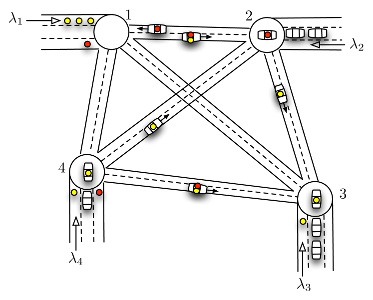
In this paper we study vehicle routing algorithms for a novel model of urban transportation system, which involves blending customer-driven vehicles with a taxi service. Our proposed car-share system is an example of a Mobility-on-Demand (MOD) system, and aims at providing urban dwellers with the tailored service of a private automobile, while utilizing limited urban land more efficiently (e.g., by minimizing the automobiles that sit unused) [1]. In our system, a customer arrives at one of many designated stations and is transported to any other designated station, either by driving themselves, or by being driven by an employed driver. The system allows for one way trips, so that customers do not have to return to the same stations from which they picked up their vehicles. In a typical one way car-share system (e.g. Car2Go) it has been observed empirically [2], and shown analytically [3], that vehicles become unbalanced, accumulating at popular destinations and becoming depleted at less popular ones. Our proposed system addresses this problem by employing rebalancing drivers to drive vehicles from the popular destinations to the unpopular destinations. However, with this approach the rebalancing drivers themselves become unbalanced, and hence we need to “rebalance the rebalancers” by letting them travel back to the popular destinations with a customer. In such a trip, the rebalancing driver operates the vehicle as a taxi, driving the customer to their desired destination. The system is illustrated in Fig. 1. The main difficulty in such a system, and the focus of this paper, is how to determine the rebalancing trips and the taxi trips in order to minimize wasted trips, while providing the best possible customer experience.

Specifically, the contribution of this paper is twofold: we study routing algorithms for the MOD system illustrated in Fig. 1 that (1) minimize the number of rebalancing vehicles traveling in the network, (2) minimize the number of drivers needed, and (3) ensure that the number of waiting customers remains bounded. Second, leveraging our analysis, we determine the relation between the minimum number of drivers needed and the minimum number of vehicles needed to ensure stability in the system; these relations would provide a system designer with essential structural insights to develop business models. Interestingly, our simulations suggest that, in Euclidean network topologies, one would need between 1/3 and 1/4 as many drivers as vehicles, and that this fraction decreases to about 1/5 if one allows up to 3-4 drivers to take a trip with a customer.

This paper builds upon the previous work of the authors in designing optimal rebalancing policies for MOD systems leveraging autonomous operation of the vehicles [4, 3], i.e., without the need of human drivers. On the contrary, the system proposed in this paper would use technology that is available today (i.e., by employing human drivers instead of autonomous cars), and our finding are readily applicable to existing one-way car-share systems, which already employ drivers to rebalance cars using heuristic methods [2]. Furthermore, by comparing the results in this paper with those in [4], one can quantitatively assess the relative benefits of “hi-tech” autonomous MOD systems versus “low-tech” driver-based MOD systems. The problem addressed in this paper has also many characteristics in common with the well-known Dynamic Traffic Assignment (DTA) problem [5, 6, 7, 8]. The key difference between rebalancing in MOD systems and the DTA problem is that in the former the optimization is over the empty vehicle trips (i.e., the rebalancing trips) rather than the passenger carrying trips.

The rest of the paper is structured as follows. In Section II we present a model for our system with customers, vehicles, and drivers represented as a continuous fluid, and we formally state the problem of rebalancing the vehicles and the drivers. In Section III we (i) study the well-posedness of the model and characterize its set of equilibria; (ii) determine the minimum number of vehicles and drivers needed to meet the customer demand; and (iii) show that with rebalancing vehicles and drivers the system is indeed locally stable (i.e., stable within a neighborhood of the nominal conditions). In Section IV we show how to optimally route the rebalancing vehicles and drivers so that stability (in terms of boundedness of the number of waiting customers) is ensured while minimizing the number of rebalancing vehicles traveling in the network and the number of rebalancing drivers needed; remarkably, these two objectives are aligned, and one can find the optimal rebalancing strategy by solving two decoupled linear programs. In Section V we study the relation between the minimum number of drivers needed and the minimum number of vehicles needed. Finally, in Section VI we give conclusions and discuss future research directions.

Figure 1: At each station there are three queues: customers (yellow dots), drivers (red dots), and vehicles (small car icons). There are three modes of use for a car: A customer can drive a car between stations; a customer can be driven between stations by a driver; or, a driver can drive a car between stations to rebalance.

TABLE I: Description of notation for station $i$

	Definition
$c_{i}$	number of customers at station $i$
$v_{i}$	number of vehicles at station $i$
$r_{i}$	number of drivers at station $i$
$\lambda_{i}$	rate of arrival of customers at station $i$
$\mu_{i}$	departure rate from station $i$
$T_{ij}$	travel time from station $i$ to station $j$
$p_{ij}$	fraction of customers at station $i$ destined for station $j$
$\alpha_{ij}$	rate of rebalancing vehicles from station $i$ to station $j$
$\gamma_{i}$	$\sum_{j}\alpha_{ij}$
$\beta_{ij}$	rate of rebalancing drivers from station $i$ to station $j$
$f_{ij}$	fraction of customers traveling from $i$ to $j$ willing
	to use taxis
$H(\cdot)$	Heaviside function

II Modeling the Mobility-on-Demand System

In our prior work [3] we proposed a fluid model for mobility-on-demand systems and formulated a policy to optimally rebalance vehicles assuming that they could operate autonomously. In this paper we consider rebalancing the vehicles through the use of dedicated personnel that are employed to drive the vehicles. In this section we extend the fluid model in [3] to capture the later scenario.

Basic model: The model in [3] can be formalized as follows. Consider a set of $n$ stations, $\mathcal{N}=\{1,\ldots,n\}$, defined over an extended geographical area (see Figure 1). Since the model is a fluid approximation, the number of customers, vehicles, and drivers are represented by real numbers. Customers arrive at station $i$ at a constant rate $\lambda_{i}\in{\mathbb{R}}_{>0}$. The number of customers at station $i$ at time $t$ is $c_{i}(t)\in{\mathbb{R}}_{\geq 0}$, and the number of vehicles waiting idle at station $i$ at time $t$ is $v_{i}(t)\in{\mathbb{R}}_{\geq 0}$. The total number of vehicles in the system is $V\in{\mathbb{R}}_{>0}$. The fraction of customers at station $i$ whose destination is station $j$ is $p_{ij}$ (where $p_{ij}\in{\mathbb{R}}_{\geq 0}$, $p_{ii}=0$, and $\sum_{j}p_{ij}=1$). The travel time from station $i$ to station $j$ is $T_{ij}\in{\mathbb{R}}_{\geq 0}$. When there are both customers and vehicles at station $i$ (i.e., $c_{i}(t)>0$ and $v_{i}(t)>0$), then the rate at which customers (and hence vehicles) leave station $i$ is $\mu_{i}$; when, instead, $c_{i}(t)=0$ but $v_{i}(t)>0$ the departure rate is $\lambda_{i}$. A necessary condition for the total number of customers at station $i$ to remain bounded is that $\mu_{i}\geq\lambda_{i}$; we will assume $\mu_{i}>\lambda_{i}$ throughout the paper (the case $\mu_{i}=\lambda_{i}$ can be addressed with techniques similar to the ones introduced in this paper and is omitted).

From [3], we showed that a station is in need of rebalancing if $-\lambda_{i}+\sum_{j\neq i}\lambda_{j}p_{ji}\neq 0$. This can be easily understood by noting that $\lambda_{i}$ is the rate at which vehicles leave station $i$, while $\sum_{j\neq i}\lambda_{j}p_{ji}$ is the rate at which vehicles arrive at station $i$. In what follows we assume that

$$-\lambda_{i}+\sum_{j\neq i}\lambda_{j}p_{ji}\neq 0\quad\text{for all $i\in\mathcal{N}$},$$

and thus each station is in need of rebalancing. We comment further on this assumption in Remark III.3.

Rebalancing vehicles: In order to rebalance the number of vehicles $v_{i}(t)$ at each station, vehicles without customers will be driven between stations using hired human drivers. The number of drivers waiting at station $i$ is $r_{i}(t)\in{\mathbb{R}}_{\geq 0}$ and the total number of drivers in the system is $R\in{\mathbb{R}}_{>0}$. In order to send a vehicle without a customer on a rebalancing trip from station $i$ to station $j$, there must be a driver present at station $i$. We let $\alpha_{ij}\in{\mathbb{R}}_{\geq 0}$ denote the rate at which we send vehicles from station $i$ to station $j$ when vehicles and drivers are available at station $i$. The total rate at which station $i$ sends vehicles without customers is $\gamma_{i}:=\sum_{j}\alpha_{ij}$, where $\alpha_{ii}=0$. We let $\alpha$ denote the matrix with entries given by $\alpha_{ij}$. These trips are shown in Figure 1 as vehicles with red dots in them.

Rebalancing drivers: Finally, we must rebalance the drivers in the network, as they will tend to accumulate at some stations and become depleted at others. This is done as follows. If a driver would like to make a trip from station $i$ to station $j$, it can drive a car for a customer on a trip from $i$ to $j$, thereby acting as a taxi driver for that trip. This allows the driver to make the journey from station $i$ to station $j$ by “hitching a ride” on a passenger-carrying trip, but without negatively affecting the customer experience. We quantify this using two sets of variables. The variables $\beta_{ij}\in{\mathbb{R}}_{\geq 0}$ give the rate at which drivers are sent from station $i$ to station $j$ when there are idle drivers available at station $i$. We let $\beta$ denote the matrix with entries given by $\beta_{ij}$ and assume $\beta_{ii}=0$.

The quantities $f_{ij}\in(0,1]$ give the fraction of customers making the trip from station $i$ to $j$ that would be willing to use the taxi mode of service on their trip. The remaining fraction of customers $1-f_{ij}$ would prefer to drive themselves on their trip. Thus, $f_{ij}$ imposes a constraint on the largest value of $\beta_{ij}$. In what follows we assume that the $f_{ij}$ are such that there are enough customer trips available to rebalance the drivers. In Proposition III.4 we give a necessary and sufficient condition on the $f_{ij}$ such that this is true. These trips are shown in Figure 1 as vehicles with red and yellow dots in them.

The notation is summarized in Table I.

We are now ready to write the differential equations governing the evolution of the number of vehicles, customers, and drivers at each station. In order to write the expressions more compactly, we introduce the following notation:

$$v_{i}:=v_{i}(t),\quad c_{i}:=c_{i}(t),\quad r_{i}:=r_{i}(t),$$

$$v_{j}^{i}:=v_{j}(t-T_{ji}),\quad c_{j}^{i}:=c_{j}(t-T_{ji}),\quad r_{j}^{i}:=r_{j}^{i}(t-T_{ij}).$$

(In other words, $v_{j}^{i}$ denotes the number of vehicles that were present at station $j$, specifically $T_{ji}$ time units prior to the current time.) Then, we can write the customer dynamics at station $i$ as

$$\dot{c}_{i}=\begin{cases}\lambda_{i},&\text{if $v_{i}=0$},\\ 0,&\text{if $v_{i}>0$ and $c_{i}=0$},\\ \lambda_{i}-\mu_{i},&\text{if $v_{i}>0$ and $c_{i}>0$}.\end{cases}$$

Defining the Heaviside function as

$$H(x):=\left\{\begin{array}[]{rl}1,&\mbox{ if $x>0$},\\ 0,&\mbox{ otherwise},\end{array}\right.$$

the customer dynamics can be written as

$$\dot{c}_{i}=\lambda_{i}\big{(}1-H(v_{i})\big{)}+(\lambda_{i}-\mu_{i})H(c_{i})H(v_{i}).$$

The rate of change of vehicles at station $i$ can be written as the sum of four components:

1. the rate at which customer-carrying vehicles depart station $i$:

   $$\begin{cases}0,&\text{if $v_{i}=0$}\\ -\lambda_{i},&\text{if $v_{i}>0$ and $c_{i}=0$},\\ -\mu_{i},&\text{if $v_{i}>0$ and $c_{i}>0$},\end{cases}$$

   which can be written more compactly as $-\lambda_{i}H(v_{i})+(\lambda_{i}-\mu_{i})H(c_{i})H(v_{i});$

2. the rate at which customer-carrying vehicles arrive at station $i$:

   $$\sum_{j\neq i}p_{ji}\,\Bigl{(}\lambda_{j}H(v_{j}^{i})-(\lambda_{j}-\mu_{j})H(c_{j}^{i})H(v_{j}^{i})\Bigr{)};$$

3. the rate at which vehicles without a customer (rebalancing vehicles) depart station $i$, given by $-\gamma_{i}H(v_{i})H(r_{i})$;

4. the rate at which vehicles without a customer (rebalancing vehicles) arrive at station $i$, given by $\sum_{j\neq i}\alpha_{ji}H(v_{j}^{i})H(r_{j}^{i})$.

Thus, the vehicle dynamics can be written as

$$\dot{v}_{i}=-\lambda_{i}H(v_{i})+(\lambda_{i}-\mu_{i})H(c_{i})H(v_{i})\\ +\sum_{j\neq i}p_{ji}\,\Bigl{(}\lambda_{j}H(v_{j}^{i})-(\lambda_{j}-\mu_{j})H(c_{j}^{i})H(v_{j}^{i})\Bigr{)}\\ -\gamma_{i}H(v_{i})H(r_{i})+\sum_{j\neq i}\alpha_{ji}H(v_{j}^{i})H(r_{j}^{i}),$$

Finally, the dynamics for the drivers contains four components. The first two components are identical to those of the rebalancing vehicles, given by 3) and 4) above. (This is due to the fact that each rebalancing vehicle contains a driver). The third component is the rate at which rebalancing drivers depart station $i$ (by driving customer carrying vehicles): $-\sum_{j\neq i}\beta_{ij}H(v_{i})H(r_{i})$. The fourth term is the rate at which rebalancing drivers arrive at station $i$ with a customer: $\sum_{j\neq i}\beta_{ji}H(v_{j}^{i})H(r_{j}^{i})$. Since drivers rebalance by driving vehicles on customer trips, we have from the customer dynamics $\dot{c}_{i}$ that

$$\beta_{ij}\leq\begin{cases}f_{ij}\lambda_{i}p_{ij}&\text{if $c_{i}=0$}\\ f_{ij}\mu_{i}p_{ij}&\text{if $c_{i}>0$}\\ \end{cases}$$

However, we will consider fixed values of $\beta_{ij}$, and since $\mu_{i}>\lambda_{i}$, we simply need to enforce the more stringent constraint $\beta_{ij}\leq f_{ij}\lambda_{i}p_{ij}$.

Therefore, the $\dot{r}_{i}$ dynamics can be written as

$$\dot{r}_{i}=-\gamma_{i}H(v_{i})H(r_{i})+\sum_{j\neq i}\alpha_{ji}H(v_{j}^{i})H(r_{j}^{i})\\ -\sum_{j\neq i}\beta_{ij}H(v_{i})H(r_{i})+\sum_{j\neq i}\beta_{ji}H(v_{j}^{i})H(r_{j}^{i}).$$

Putting everything together, we can write a set of nonlinear, time-delay differential equations describing the evolution of customers and vehicles in the system as

$$\begin{split}\dot{c}_{i}=&\lambda_{i}\big{(}1-H(v_{i})\big{)}+(\lambda_{i}-\mu_{i})H(c_{i})H(v_{i}),\\ \dot{v}_{i}=&-\lambda_{i}H(v_{i})+(\lambda_{i}-\mu_{i})H(c_{i})H(v_{i})+\\ &\sum_{j\neq i}p_{ji}\,\Bigl{(}\lambda_{j}H(v_{j}^{i})-(\lambda_{j}-\mu_{j})H(c_{j}^{i})H(v_{j}^{i})\Bigr{)}\\ &\qquad-\gamma_{i}H(v_{i})H(r_{i})+\sum_{j\neq i}\alpha_{ji}H(v_{j}^{i})H(r_{j}^{i}),\\ \dot{r}_{i}=&-\gamma_{i}H(v_{i})H(r_{i})+\sum_{j\neq i}\alpha_{ji}H(v_{j}^{i})H(r_{j}^{i})\\ &-\sum_{j\neq i}\beta_{ij}H(v_{i})H(r_{i})+\sum_{j\neq i}\beta_{ji}H(v_{j}^{i})H(r_{j}^{i}).\end{split}$$ (1)

where $t\geq 0$; the initial conditions satisfy $c_{i}(\tau)=0,\,v_{i}(\tau)=0$, $r_{i}(\tau)=0$ for $\tau\in[-\max_{i,j}\,T_{ij},\,0)$, $c_{i}(0)\in{\mathbb{R}}_{\geq 0},\,v_{i}(0)\in{\mathbb{R}}_{\geq 0}$ with $v_{i}(0)>0$ for at least one $i\in\mathcal{N}$, $r_{i}(0)\in{\mathbb{R}}_{\geq 0}$ with $r_{i}(0)>0$ for at least one $i\in\mathcal{N}$, and $\sum_{i}\,v_{i}(0)=V$ and $\sum_{i}r_{i}(0)=R$. The optimization variables $\alpha$ and $\beta$ are constrained as follows:

$$0\leq \,\beta_{ij}\leq f_{ij}\lambda_{i}p_{ij}$$

$$0\leq \,\alpha_{ij}.$$

The problem we wish to solve is as follows: find an optimal vehicle rebalancing assignment $\alpha$ and driver rebalancing assignment $\beta$ that simultaneously

1. minimizes the number of rebalancing vehicles traveling in the network,

2. minimizes the number of drivers needed, and

3. ensures that the number of waiting customers remains bounded.

Note that this is a multi-objective optimization, and thus it is not clear that one can both minimize the number of rebalancing vehicles in the network and the number of drivers needed. However, it will turn out that these two objectives are aligned, and one can find an assignment $(\alpha,\beta)$ that minimizes both objectives.

III Well-posedness, Equilibria, and Stability of Fluid Model

In this section we first discuss the well-posedness of model (1) by showing two important properties, namely existence of solutions and invariance of the number of vehicles and rebalancing drivers along system trajectories. Then, we characterize the equilibria, we determine the minimum number of vehicles and drivers to ensure their existence, and we give a necessary and sufficient condition on the “user’s preference” $f_{ij}$ such that there are enough customer trips available to rebalance the drivers. Finally, we show that rebalancing vehicles and drivers give rise to equilibria that are locally (i.e., within a neighborhood of the nominal conditions) stable.

III-A Well-posedness

The fluid model (1) is nonlinear, time-delayed, and the right-hand side is discontinuous. Due to the discontinuity, we need to analyze the model within the framework of Filippov solutions (see, e.g., [9]). The following proposition verifies that the fluid model is well-posed.

Proposition III.1 (Well-posedness of fluid model).

For the fluid model (1), the following hold:

1. For every initial condition, there exist continuous functions $c_{i}(t):{\mathbb{R}}\to{\mathbb{R}}_{\geq 0}$, $v_{i}(t):{\mathbb{R}}\to{\mathbb{R}}_{\geq 0}$, and $r_{i}(t):{\mathbb{R}}\to{\mathbb{R}}_{\geq 0}$ $i\in\mathcal{N}$, satisfying the differential equations (1) in the Filippov sense.

2. The total number of vehicles and rebalancing drivers is invariant for $t\geq 0$ and is equal, respectively, to $V=\sum_{i}\,v_{i}(0)$ and $R=\sum_{i}\,r_{i}(0)$.

Proof.

To prove the first claim, it can be checked that all assumptions of Theorem II-1 in [10] for the existence of Filippov solutions to time-delay differential equations with discontinuous right-hand side are satisfied, and the claim follows.

As for the second claim, the proof of the invariance of the number of vehicles is virtually identical to the one of Proposition 3.1 in [3] and is omitted in the interest of brevity. We prove next the invariance of the number of rebalancing drivers. Let $r_{ij}(t)$, where $t\geq 0$, be the number of rebalancing drivers in-transit from station $i$ to station $j$ (i.e., the rebalancing drivers for which the last station visited is $i$ and the next station they will visit is $j$). Clearly, $r_{ii}(t)=0$. Now, the total number $R(t)$ of rebalancing drivers in the system at time $t\geq 0$ is given, by definition, by $R(t)=\sum_{i=1}^{n}\,r_{i}(t)+\sum_{i,j}\,r_{ij}(t)$. The number of in-transit rebalancing drivers at time $t$ is given by the integral over the last $T_{ij}$ time units (i.e., the time to get from station $i$ to station $j$) of the rebalancing driver departure rate from station $i$ to station $j$. Such departure rate is the sum of the departure rate of rebalancing vehicles (since each rebalancing vehicle contains a rebalancing driver) and of the departure rate of rebalancing drivers that drive customer-carrying vehicles; hence, one can express $r_{ij}(t)$ as

$$r_{ij}(t)=\int_{t-T_{ij}}^{t}\underbrace{\alpha_{ij}H(v_{i}(\tau))H(r_{i}(\tau))}_{\text{rate of drivers on rebalancing vehicles}}\,+\\ \underbrace{\beta_{ij}H(v_{i}(\tau))H(r_{i}(\tau))}_{\text{rate of drivers on customer-carrying vehicles}}\,d\tau.$$ (2)

By applying the Leibniz integral rule, one can write

$$\begin{split}\dot{r}_{ij}(t)&=(\alpha_{ij}+\beta_{ij})\Bigl{(}H(v_{i})H(r_{i})-H(v_{i}^{j})H(r_{i}^{j})\Bigr{)}.\end{split}$$

Therefore, one immediately obtains, for $t\geq 0$,

$$\dot{R}(t) =\sum_{i=1}^{n}\dot{r}_{i}(t)+\sum_{i=1}^{n}\sum_{j=1}^{n}\dot{r}_{ij}(t)$$

$$=-\sum_{i=1}^{n}\sum_{j=1}^{n}(\alpha_{ij}+\beta_{ij})H(v_{i})H(r_{i})\,+$$

$$\qquad\sum_{i=1}^{n}\sum_{j=1}^{n}(\alpha_{ji}+\beta_{ji})H(v_{j}^{i})H(r_{j}^{i})\,+\sum_{i=1}^{n}\sum_{j=1}^{n}\dot{r}_{ij}(t)$$

$$=0.$$

This proves the claim. ∎

III-B Equilibria

The following result characterizes the equilibria of model (1). Recall that no station is exactly balanced, and thus $-\lambda_{i}+\sum_{j\neq i}\lambda_{j}p_{ji}\neq 0$, for all $i\in\mathcal{N}$.

Theorem III.2 (Existence of equilibria).

Let $\mathcal{A}\times\mathcal{B}$ be the set of assignments $(\alpha,\beta)$ that verify the equations

$$\sum_{j\neq i}(\alpha_{ij}-\alpha_{ji}) =D_{i},$$ (3)

$$\sum_{j\neq i}(\beta_{ij}-\beta_{ji}) =-D_{i},$$ (4)

for each $i\in\mathcal{N}$, where $D_{i}:=-\lambda_{i}+\sum_{j\neq i}\lambda_{j}p_{ji}$. Moreover, let

$$V_{\alpha} :=\sum_{i,j}\,T_{ij}\,(p_{ij}\lambda_{i}+\alpha_{ij}),\quad\text{and}$$

$$R_{\alpha,\beta} :=\sum_{i,j}\,T_{ij}\,(\alpha_{ij}+\beta_{ij}).$$

If $(\alpha,\beta)\notin\mathcal{A}\times\mathcal{B}$, then no equilibrium exists. If $(\alpha,\beta)\in\mathcal{A}\times\mathcal{B}$, there are two cases:

1. If $V>V_{\alpha}$ and $R>R_{\alpha,\beta}$, then the set of equilibria is

   $$c_{i}=0,\qquad v_{i}>0,\quad r_{i}>0\qquad\forall\;i\in\mathcal{N},$$

   where $\sum_{i}v_{i}=V-V_{\alpha}$ and $\sum_{i}r_{i}=R-R_{\alpha,\beta}$.

2. If $V\leq V_{\alpha}$ or $R\leq R_{\alpha,\beta}$, then no equilibrium exists.

Proof.

To prove the theorem, we set $\dot{c}_{i}=0$, $\dot{v}_{i}=0$, and $\dot{r}_{i}=0$ for all $i\in\mathcal{N}$. From the $\dot{c}_{i}=0$ equations we obtain

$$\lambda_{i}=\lambda_{i}H(v_{i})-(\lambda_{i}-\mu_{i})H(v_{i})H(c_{i}).$$ (5)

Since $\lambda_{i}<\mu_{i}$, the above equations have a solution only if

$$c_{i}=0\quad\text{and}\quad v_{i}>0\quad\text{$\forall\;i\in\mathcal{N}$}.$$

Setting $\dot{v}_{i}=0$, combined with (5) and the fact that in equilibrium $c_{i}=0$ and $v_{i}$ is a positive constant, we obtain

$$\sum_{j\neq i}\big{(}\alpha_{ij}H(r_{i})-\alpha_{ji}H(r_{j})\big{)}=D_{i},$$ (6)

where $D_{i}:=-\lambda_{i}+\sum_{j\neq i}\lambda_{j}p_{ji}$. Finally, setting $\dot{r}_{i}=0$, combined with the fact that $v_{i}>0$ in equilibrium, we obtain

$$\sum_{j\neq i}\big{(}\alpha_{ij}H(r_{i})-\alpha_{ji}H(r_{j})\big{)}$$ (7)

$$=-\sum_{j\neq i}\big{(}\alpha_{ij}H(r_{i})-\alpha_{ji}H(r_{j})\big{)}=-D_{i}.$$

Now, consider any station $i$, and note that by assumption we have $D_{i}\neq 0$. If $D_{i}>0$ then from (6) we see that $r_{i}>0$ in equilibrium. Alternatively, if $D_{i}<0$, then from (7) we see that $r_{i}>0$. Therefore, in equilibrium $r_{i}>0$.

We have shown that all equilibria are of the form $c_{i}=0$, $v_{i}>0$, and $r_{i}>0$, for each $i\in\mathcal{N}$. A necessary condition for the existence of equilibria is that the rebalancing assignments $\alpha$ and $\beta$ can be chosen such that they lie in the set $\mathcal{A}\times\mathcal{B}$ of assignments that verify

$$\sum_{j\neq i}(\alpha_{ij}-\alpha_{ji}) =D_{i},$$

$$\sum_{j\neq i}(\beta_{ij}-\beta_{ji}) =-D_{i},$$

for each $i\in\mathcal{N}$. If $(\alpha,\beta)\notin\mathcal{A}\times\mathcal{B}$, then no equilibrium exists and the first claim is proven.

Assume now that $(\alpha,\beta)\in\mathcal{A}\times\mathcal{B}$ and assume that $V>V_{\alpha}$ and $R>R_{\alpha,\beta}$. We need to show that $c_{i}=0$, $v_{i}>0$, and $r_{i}>0$ for all $i\in\mathcal{N}$ are indeed valid equilibria. The necessary conditions in equations (3) and (4) are clearly satisfied and thus we simply need to verify that the number of vehicles and drivers are sufficient to support the equilibrium configuration. But, we showed in [3] that $V_{\alpha}$ is exactly the equilibrium number of vehicles in transit. Similarly, from equation (2) we can verify that $R_{\alpha,\beta}$ is the equilibrium number of drivers in transit. This, together with the invariance result in Theorem III.1, shows the second claim.

Finally, we can show that if $(\alpha,\beta)\in\mathcal{A}\times\mathcal{B}$ but $V\leq V_{\alpha}$ or $R\leq R_{\alpha,\beta}$, then no equilibrium exists, by arguing that in this case there is not a sufficient number of vehicles and/or drivers to support the equilibrium. ∎

Remark III.3 (Balanced stations case).

We have assumed that $D_{i}=-\lambda_{i}+\sum_{j\neq i}\lambda_{j}p_{ji}\neq 0$ for each station $i$. This assumption removes the pathological case that a station is perfectly balanced and does not need any rebalancing effort. In the case that $D_{i}=0$ for a station, then $r_{i}=0$ becomes a valid equilibrium. Due to space constraints we have omitted a full treatment of the $D_{i}=0$ case in this presentation. $\bullet$

One question remains; does there always exist an assignment $(\alpha,\beta)\in\mathcal{A}\times\mathcal{B}$ that satisfies the constraints $\alpha_{ij}\geq 0$, and $0\leq\beta_{ij}\leq f_{ij}\lambda_{i}p_{ij}$ for each $i,j\in\mathcal{N}$? We call such an assignment feasible. It is straightforward to verify that a feasible assignment for $\alpha$ always exists, since the variables are constrained only to be non-negative [3]. The $\beta$ variables, however, are bounded from above (that is, they have finite capacities), and thus it is not clear whether there exists a feasible $\beta$ assignment. The following result gives a standard condition for the existence of a feasible assignment (see, for example [11, p. 220] and a consequence of this condition.

Proposition III.4 (Existence of a feasible assignment).

A feasible assignment $(\alpha,\beta)$ exists if and only if,

$$-\sum_{i\in S}D_{i}\leq\sum_{i\in S,j\notin S}f_{ij}\lambda_{i}p_{ij}\quad\text{for every set $S\subseteq\mathcal{N}$},$$ (8)

where $D_{i}=-\lambda_{i}+\sum_{j\neq i}\lambda_{j}p_{ji}$. As a consequence, if $f_{ij}=1$ for all $i,j,\in\mathcal{N}$, then a feasible assignment always exists.

Proof.

The condition (8) is a standard condition for the existence of a feasible solution in a minimum cost flow problem [11, p. 220].

Now we show that if $f_{ij}=1$ for all $i,j\in\mathcal{N}$, then (8) is satisfied. Take any subset $S\subseteq\mathcal{N}$ and let us show that

$$\sum_{i\in S}D_{i}+\sum_{i\in S,j\notin S}\lambda_{i}p_{ij}\geq 0.$$

From the definition of $D_{i}$, the left-hand side of the above expression can be written as

$$-\sum_{i\in S}\lambda_{i}+\sum_{i\in S,j\in\mathcal{N}}\lambda_{j}p_{ji}+\sum_{i\in S,j\notin S}\lambda_{i}p_{ij}$$

$$=-\sum_{i,j\in S}\lambda_{i}p_{ij}+\sum_{i\in S,j\in\mathcal{N}}\lambda_{j}p_{ji}$$

$$=-\sum_{i,j\in S}\lambda_{i}p_{ij}+\sum_{i\in S,j\in\mathcal{N}}\lambda_{j}p_{ji}$$

$$=\sum_{i\notin S,j\in S}\lambda_{i}p_{ij}\geq 0.$$

This proves the feasibility when $f_{ij}=0$ for all $i,j\in\mathcal{N}$. ∎

III-C Stability of Equilibria

In this section we investigate the (local) stability of the equilibria of our model. We consider the following notion of local stability. Let $(\alpha,\beta)\in\mathcal{A}\times\mathcal{B}$ and assume $V>V_{\alpha}$ and $R>R_{\alpha,\beta}$ (this is a necessary and sufficient condition to have equilibria, see Theorem III.2). We say that the (non-empty) set of equilibria

$$\begin{split}&\mathcal{E}_{\alpha,\beta}:=\big{\{}(\mathbf{c},\mathbf{v},\mathbf{r})\in{\mathbb{R}}^{3n}\,\big{|}\,c_{i}=0,v_{i}>0,r_{i}>0\text{ for all }\\ &\qquad i\in\mathcal{N},\text{ and }\sum_{i}v_{i}=V-V_{\alpha}\text{ and }\sum_{i}r_{i}=R-R_{\alpha,\beta}\big{\}}\end{split}$$ (9)

is locally asymptotically stable if for any equilibrium $(\underline{\mathbf{c}},\underline{\mathbf{v}},\underline{\mathbf{r}})\in\mathcal{E}_{\alpha,\beta}$ there exists a neighborhood $\mathcal{B}^{\delta}_{\alpha,\beta}(\underline{\mathbf{c}},\underline{\mathbf{v}},\underline{\mathbf{r}}):=\{(\mathbf{c},\mathbf{v},\mathbf{r})\in{\mathbb{R}}^{3n}\,|\,c_{i}\geq 0,v_{i}\geq 0,r_{i}\geq 0\text{ for all }i\in\mathcal{N},\|(\mathbf{c}-\underline{\mathbf{c}},\mathbf{\mathbf{v}}-\underline{\mathbf{v}},\mathbf{\mathbf{r}}-\underline{\mathbf{r}})\|<\delta,\text{ and }\sum v_{i}=V-V_{\alpha}\text{ and }\sum r_{i}=R-R_{\alpha,\beta}\}$ such that every evolution of model (1) starting at

$$\begin{split}&c_{i}(\tau)=\underline{c}_{i}\text{ for }\tau\in[-\max_{i,j}T_{ij},\,0)\\ &v_{i}(\tau)=\underline{v}_{i}\text{ for }\tau\in[-\max_{i,j}T_{ij},\,0)\\ &r_{i}(\tau)=\underline{r}_{i}\text{ for }\tau\in[-\max_{i,j}T_{ij},\,0)\\ &(\mathbf{c}(0),\mathbf{v}(0),\mathbf{r}(0))\in\mathcal{B}^{\delta}_{\alpha,\beta}(\underline{\mathbf{c}},\underline{\mathbf{v}},\underline{\mathbf{r}}))\end{split}$$ (10)

has a limit which belongs to the equilibrium set. In other words, $\big{(}\lim_{t\to+\infty}\mathbf{c}(t),\lim_{t\to+\infty}\mathbf{v}(t),\lim_{t\to+\infty}\mathbf{r}(t)\big{)}\in\mathcal{E}_{\alpha,\beta}$. The next theorem characterizes stability.

Theorem III.5 (Stability of equilibria).

Let $(\alpha,\beta)\in\mathcal{A}\times\mathcal{B}$ be a feasible assignment, and assume $V>V_{\alpha}$ and $R>R_{\alpha,\beta}$; then, the set of equilibria $\mathcal{E}_{\alpha,\beta}$ is locally asymptotically stable.

Proof.

Consider an equilibrium $(\underline{\mathbf{c}},\underline{\mathbf{v}},\underline{\mathbf{r}})\in\mathcal{E}_{\alpha,\beta}$ (note that $\underline{\mathbf{c}}=\mathbf{0}$ by Theorem III.2). We now prove that every evolution of model (1) starting at

$$\begin{split}&c_{i}(\tau)=0\text{ for }\tau\in[-\max_{i,j}T_{ij},\,0)\\ &v_{i}(\tau)=\underline{v}_{i}\text{ for }\tau\in[-\max_{i,j}T_{ij},\,0)\\ &r_{i}(\tau)=\underline{r}_{i}\text{ for }\tau\in[-\max_{i,j}T_{ij},\,0)\\ &(\mathbf{c}(0),\mathbf{v}(0),\mathbf{r}(0))\text{ such that }(1)\,\,0\leq c_{i}(0)<v_{i}(0)\,\,\forall i,\\ &\qquad\qquad(2)\,\,0<r_{i}(0)\,\,\forall i,(3)\,\,\sum v_{i}(0)=V-V_{\alpha},\\ &\qquad\qquad\text{and }(4)\,\,\sum r_{i}(0)=R-R_{\alpha,\beta}\end{split}$$ (11)

has a limit which belongs to the equilibrium set. The claim of the theorem will then be an easy consequence of this statement.

We start by observing the following fact. Assume that $v_{i}(\tau)>0$ and $r_{i}(\tau)>0$ for all $\tau\in[-\max_{i,j}T_{ij},\,t]$, then at time $t$ the differential equations read $\dot{c}_{i}(t)=(\lambda_{i}-\mu_{i})H(c_{i}(t))$, for all $i\in\mathcal{N}$; recalling that, by Theorem III.2, it must hold $-\lambda_{i}+\sum_{j\neq i}\lambda_{j}p_{ji}-\gamma_{i}+\sum_{j\neq i}\alpha_{ji}=0$, one can write

$$\begin{split}\dot{v}_{i}(t)&=-\lambda_{i}+(\lambda_{i}-\mu_{i})H(c_{i})+\sum_{j\neq i}p_{ji}\Bigl{(}\lambda_{j}-\\ &\qquad\qquad(\lambda_{j}-\mu_{j})H(c_{j}^{i})\Bigr{)}-\gamma_{i}+\sum_{j\neq i}\alpha_{ji}\\ &=(\lambda_{i}-\mu_{i})H(c_{i})-\sum_{j\neq i}p_{ji}(\lambda_{j}-\mu_{j})H(c_{j}^{i})\\ &\geq(\lambda_{i}-\mu_{i})H(c_{i}),\quad\text{for all }i\in\mathcal{N}.\end{split}$$

Also, since by Theorem III.2, it must hold - $\sum_{j\neq i}(\alpha_{ij}-\alpha_{ji})+\sum_{j\neq i}(\beta_{ji}-\beta_{ij})=0$, one can write

$$\begin{split}\dot{r}_{i}(t)&=-\sum_{j\neq i}(\alpha_{ij}+\beta_{ij})+\sum_{j\neq i}(\alpha_{ji}+\beta_{ji})=0.\end{split}$$

Since $v_{i}(\tau)>0$ for all $\tau\in[-\max_{i,j}T_{ij},\,0]$, and since $v_{i}(0)>c_{i}(0)$ for all $i\in\mathcal{N}$, we conclude that no $v_{i}(t)$ and $r_{i}(t)$ can reach the value $0$ before the corresponding number of customers $c_{i}(t)$ has reached the value $0$. However, once $c_{i}(t)$ reaches the value $0$ (after a time interval $c_{i}(0)/(\mu_{i}-\lambda_{i})$), the time derivative $\dot{v}_{i}(t)$ is larger than or equal to zero. This implies that when the initial conditions satisfy (11), then $v_{i}(t)>0$ and $r_{i}(t)>0$ for all $t\geq 0$.

Since $v_{i}(t)>0$ and $r_{i}(t)>0$ for all $t\geq 0$, and since this implies that $\dot{c}_{i}(t)=(\lambda_{i}-\mu_{i})H(c_{i}(t))$ for all $i\in\mathcal{N}$ and $t\geq 0$, we conclude that all $c_{i}(t)$ will be equal to zero for all $t\geq T^{\prime}:=\max_{i}\,c_{i}(0)/(\mu_{i}-\lambda_{i})$. Then, for $t\geq T^{\prime}+\max_{ij}T_{ij}=:T^{\prime\prime}$ the differential equations become: $\dot{c}_{i}(t)=0$, $\dot{v}_{i}(t)=0$, $\dot{r}_{i}(t)=0$.

Collecting the results obtained so far, we have that $\lim_{t\to+\infty}c_{i}(t)=0$ for all $i\in\mathcal{N}$. Moreover, since $\dot{v}_{i}(t)=0$ and $\dot{r}_{i}(t)=0$ for all $t\geq T^{\prime\prime}$, the limits $\lim_{t\to+\infty}v_{i}(t)$ and $\lim_{t\to+\infty}r_{i}(t)$ exist. Finally, one has $v_{i}(t)=v_{i}(0)+\int_{0}^{t}\,\dot{v}_{i}(\tau)\,d\tau\geq v_{i}(0)+\int_{0}^{t}\,\dot{c}_{i}(\tau)\,d\tau=v_{i}(0)+c_{i}(t)-c_{i}(0)$. Since $v_{i}(0)>c_{i}(0)$, we conclude that $\lim_{t\to+\infty}v_{i}(t)>0$. Also, $\dot{r}_{i}(t)=0$ for all $t$, hence $\lim_{t\to+\infty}r_{i}(t)>0$. Thus any solution with initial conditions (11) has a limit which belongs to $\mathcal{E}_{\alpha,\beta}$ (the properties $\lim_{t\to+\infty}\sum v_{i}(t)=V-V_{\alpha}$ and $\lim_{t\to+\infty}\sum r_{i}(t)=R-R_{\alpha,\beta}$ are guaranteed by the invariance property in Proposition III.1 and the assumptions $\sum v_{i}(0)=V-V_{\alpha}$ and $\sum r_{i}(0)=R-R_{\alpha,\beta}$).

Let $\psi_{i}:=\min(\underline{r_{i}},\underline{v_{i}}\,\sin\frac{\pi}{4})$, and let $\psi_{\text{min}}:=\min_{i}\,\psi_{i}$. Then, from simple a geometric argument and from the definitions of $\psi_{i}$ and $\psi_{\text{min}}$, it follows that if one chooses $\delta=\psi_{\text{min}}$, then any solution of model (1) with initial conditions satisfying (10) has a limit which belongs to the equilibrium set. This concludes the proof. ∎

IV Optimal Rebalancing

Our objective is to find a rebalancing assignment $(\alpha,\beta)$ that simultaneously minimizes the number of rebalancing vehicles traveling in the network and the number of rebalancing drivers needed, while ensuring the existence of (locally) stable equilibria for model (1). From the previous section, we already know that the set of assignments ensuring the existence of stable equilibria is $\mathcal{A}\times\mathcal{B}$ (provided that the total number of vehicles $V$ and drivers $R$ is large enough).

The time-average number of rebalancing vehicles traveling in the network is simply given by $\sum_{i,j}T_{ij}\alpha_{ij}$. Note that in minimizing this quantity we are also minimizing the lower bound on the necessary number of vehicles $V_{\alpha}$. The time-average number of drivers in the network is given by $\sum_{i,j}T_{ij}(\alpha_{ij}+\beta_{ij})$. Note that in minimizing this quantity we are minimizing the lower bound on the necessary number of drivers $R_{\alpha,\beta}$.

Combining the two objectives with the existence of stable equilibria constraints in (3) and (4)), we obtain the following optimization:

minimize $$\sum_{i,j}T_{ij}\alpha_{ij}\;\text{and}\;\sum_{i,j}T_{ij}(\alpha_{ij}+\beta_{ij})$$

subject to $$\sum_{j\neq i}(\alpha_{ij}-\alpha_{ji})=D_{i} \forall\;i\in\mathcal{N}$$

$$\sum_{j\neq i}(\beta_{ij}-\beta_{ji})=-D_{i} \forall\;i\in\mathcal{N}$$

$$0\leq\alpha_{ij} \forall\;i,j\in\mathcal{N},$$

$$0\leq\beta_{ij}\leq f_{ij}\lambda_{i}p_{ij} \forall\;i,j\in\mathcal{N},$$

where $D_{i}=\lambda_{i}+\sum_{j\neq i}\lambda_{j}p_{ji}$, and the optimization variables are $\alpha_{ij}$ and $\beta_{ij}$, where $i,j\in\mathcal{N}$. The constraints ensure that the optimization is over the set $\mathcal{A}\times\mathcal{B}$. Note, however, that this optimization can be decoupled into an optimization over $\alpha$ and an optimization over $\beta$. Both optimizations are minimum cost flow problems [11]. The $\alpha$ optimization is identical to that presented in [3]:

minimize $$\sum_{i,j}T_{ij}\alpha_{ij}$$

subject to $$\sum_{j\neq i}(\alpha_{ij}-\alpha_{ji})=D_{i} \forall\;i\in\mathcal{N}$$

$$\alpha_{ij}\geq 0 \forall\;i,j\in\mathcal{N}.$$

The $\beta$ optimization then looks as follows:

minimize $$\sum_{i,j}T_{ij}\beta_{ij}$$

subject to $$\sum_{j\neq i}(\beta_{ij}-\beta_{ji})=-D_{i} \forall\;i\in\mathcal{N}$$

$$0\leq\beta_{ij}\leq f_{ij}\lambda_{i}p_{ij} \forall\;i,j\in\mathcal{N}.$$

The $\alpha$ optimization is an uncapacitated minimum cost flow problem and thus is always feasible. In Proposition III.4 we give conditions on the $f_{ij}$ fractions in order for the $\beta$ optimization to be feasible.

The rebalancing policy is then given by solving the two minimum cost flow problems to obtain solutions $\alpha_{ij}^{*}$ and $\beta_{ij}^{*}$. We then send empty rebalancing vehicles (along with drivers) from station $i$ to station $j$ at a rate of $\alpha^{*}_{ij}$ (when vehicles and drivers are available at station $i$). In addition, we send drivers on customer-carrying vehicles from $i$ to $j$ at a rate of $\beta^{*}_{ij}$ (when customers and vehicles are available at station $i$).

V Simulations

Figure 2: Left figure: The minimum number of vehicles and drivers. Middle figure: The ratio between the minimum number of drivers and number of vehicles. Right figure: The fraction of drivers that are performing vehicle rebalancing trips. For each fixed number of stations, $20$ trials were performed. Thick lines show the mean of the $20$ trials while thin dashed lines show the maximum and minimum over the trials.

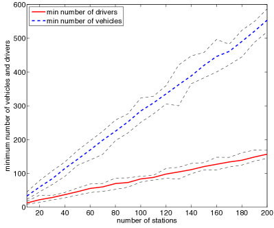
In this section we study the relation between the minimum number of drivers needed for stability $R_{\alpha,\beta}$ and the minimum number of vehicles needed $V_{\alpha}$ from Theorem III.2. To evaluate these quantities, we need to generate sample data consisting of arrival rates $\lambda_{i}$ at each station $i$, customer destination probabilities $p_{ij}$, travel times between stations $T_{ij}$, and the fraction of customers $f_{ij}$ traveling from $i$ to $j$ that are willing to be driven by a driver. We generate this data as follows: We uniformly randomly place $n$ stations in a $100\times 100$ environment, and calculate the travel times $T_{ij}$ as the Euclidean distance between stations. We uniformly randomly generate the arrival rates $\lambda_{i}$ on the interval $[0,0.05]$ arrivals per time unit. Similarly we uniformly randomly generate the destination probabilities $p_{ij}$ such that they are nonnegative and $\sum_{j}p_{ij}=1$ for each station $i$. Finally, we assume that $f_{ij}=1$ for each pair of stations in order to avoid issues with feasibility.

To solve the optimizations in Section IV for the optimal assignment $(\alpha^{*},\beta^{*})\in\mathcal{A}\times\mathcal{B}$, we use the freely available SeDuMi (Self-Dual-Minimization) toolbox.

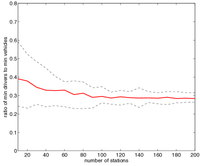
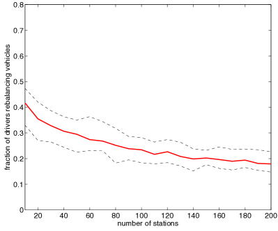
Figure 2 shows results for numbers of stations ranging from $10$ up to $200$. For each number of stations we generate $20$ random problem instances of the form described above. The thick line in each plot shows the mean over the $20$ trials while the thin dashed lines show the maximum and minimum values. The left figure shows how $V_{\alpha^{*}}$ and $R_{\alpha^{*},\beta^{*}}$ vary with the number of stations. The middle figure shows the ratio $R_{\alpha^{*},\beta^{*}}/V_{\alpha^{*}}$ as a function of the number of stations. We can see that we need between $1/3$ and $1/4$ as many drivers as we do vehicles. The right figure shows the ratio between the minimum number of rebalancing vehicles in transit and the number of drivers. This gives a measure of the fraction of drivers that are driving rebalancing vehicles (versus rebalancing themselves). It is interesting to note that this ratio is quite low, reaching approximation $1/5$ for $200$ stations.

Figure 3: Increasing the number of drivers per customer trip for $100$ station problems. Left figure: The minimum number of vehicles and drivers. Right figure: The fraction of drivers that are performing vehicle rebalancing trips.

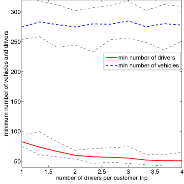
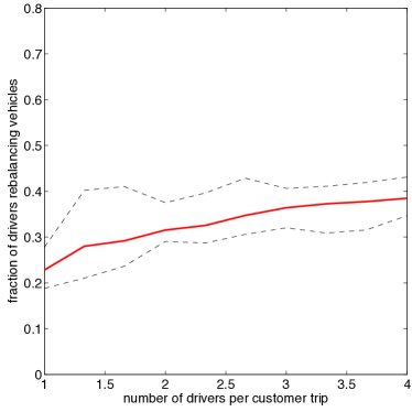
One way to increase the fraction of drivers performing vehicle rebalancing is to allow multiple drivers to take a trip with a customer. This allows drivers to take more efficient routes back to stations that are in need of drivers. In our model it corresponds to setting $f_{ij}>1$. This is explored in Figure 3 where we range $f_{ij}$ from $1$ to $4$ for $20$ problem instances on $100$ stations. We can see that as we increase $f_{ij}$ from $1$ to $4$, the number of drivers decreases from approximately $80$ to $50$, and the fraction of drivers performing vehicle rebalancing increases from under $1/4$ to nearly $2/5$.

VI Conclusions

In this paper we studied the problem of rebalancing the rebalancers in a mobility-on-demand system, which blends customer-driven vehicles with a taxi service. For a fluid model of the system, we showed that the optimal rebalancing policy can be found as the solution of two linear programs. Also, we showed that in Euclidean network topologies one would need between 1/3 and 1/4 as many drivers as vehicles, and that this fraction decreases to about 1/5 if one allows up to 3-4 drivers to take a trip with a customer. These results could have an immediate impact on existing one-way car-sharing systems such as Car2Go. For future work we plan to analyze a stochastic queueing model and study the time-varying case whereby the system’s parameters change periodically (thus modeling the day/night variations). Also, we plan to develop real-time rebalancing policies that do not require any a priori information, and to enrich our model by including uncertainty in the travel times, time windows for the customers, and capacity constraints for the roads. Finally, we are interested in using dynamic pricing to provide incentives for customers to perform rebalancing trips themselves.

Funding

This research was supported by the Future Urban Mobility project of the Singapore-MIT Alliance for Research and Technology (SMART) Center, with funding from Singapore’s National Research Foundation; and by the Office of Naval Research [grant number N000140911051].

References

- [1] W. J. Mitchell, C. E. Borroni-Bird, and L. D. Burns, Reinventing the Automobile: Personal Urban Mobility for the 21st Century. Cambridge, MA: The MIT Press, 2010.
- [2] CAR2GO, “CAR2GO Austin. Car Sharing 2.0: Great Idea for a Great City,” Tech. Rep., 2011.
- [3] M. Pavone, S. L. Smith, E. Frazzoli, and D. Rus, “Robotic load balancing for mobility-on-demand systems,” International Journal of Robotics Research, vol. 31, no. 7, pp. 839–854, 2012.
- [4] ——, “Load balancing for mobility-on-demand systems,” in Robotics: Science and Systems, Los Angeles, CA, June 2011.
- [5] D. K. Merchant and G. L. Nemhauser, “Optimality Conditions for a Dynamic Traffic Assignment Model,” Transportation Science, vol. 12, no. 3, pp. 200–207, 1978.
- [6] T. L. Friesz, J. Luque, R. L. Tobin, and B. W. Wie, “Dynamic Network Traffic Assignment Considered as a Continuous Time Optimal Control Problem,” Operations Research, vol. 37, no. 6, pp. 893–901, 1989.
- [7] A. K. Ziliaskopoulos, “A Linear Programming Model for the Single Destination System Optimum Dynamic Traffic Assignment Problem,” Transportation Science, vol. 34, no. 1, pp. 37–49, 2000.
- [8] S. Peeta and A. Ziliaskopoulos, “Foundations of Dynamic Traffic Assignment: The Past, the Present and the Future,” Networks and Spatial Economics, vol. 1, pp. 233–265, 2001.
- [9] A. F. Filippov, Differential Equations with Discontinuous Righthand Sides, ser. Mathematics and its Applications. Dordrecht, The Netherlands: Kluwer Academic Publishers, 1988, vol. 18.
- [10] G. Haddad, “Monotone trajectories of differential inclusions and functional differential inclusions with memory,” Israel Journal of Mathematics, vol. 39, no. 1-2, pp. 83 – 100, 1981.
- [11] B. Korte and J. Vygen, Combinatorial Optimization: Theory and Algorithms, 4th ed., ser. Algorithmics and Combinatorics. Springer, 2007, vol. 21.