Vacuum-excited surface plasmon polaritons

Abstract

We separate Maxwell’s equations for background media that allow for both electric and magnetic time-dependence in a generalized Lorenz gauge. In a process analogous to the dynamical Casimir effect (DCE) we discuss how surface plasmon polaritons (SPP)s can be created out of vacuum, via the time-dependent variation of a dielectric and magnetic insulator at a metal interface for TM and TE branches, respectively. We suggest how to extend currently proposed DCE experiments to set up and detect these excitations. Numerical simulations (without any approximation) indicate that vacuum excited SPPs can be of a similar magnitude to the photon creation rate in such experiments. Potential benefits of detecting vacuum excited SPPs, as opposed to DCE photons, are that parametric enhancement does not require a sealed cavity in the axial direction and the detection apparatus might be able to use simple phase matching techniques. For the case of constant permeability, $\mu$, TM branch SPPs and photons do not suffer from detuning and attenuation like TE photons.

I Introduction

Particle creation via the Schwinger-effect Schwinger (1951), in expanding universes Parker (1968) or from black hole evaporation Hawking (1974) all have yet to be confirmed. However a related effect known as the dynamical Casimir effect (DCE), first discussed by Moore Moore (1970), is in experimental reach. For the parametric oscillations of a mirror contained in a cavity the number of photons created is proportional to $\sinh^{2}(2\omega t\,v/c)$, e.g., see Dodonov (2010), where $v$ is the wall velocity and $c$ is the speed of light. To overcome the fact that the mechanical properties of the material usually imply $v/c\ll 1$, there have been proposals other than mechanical oscillations. Modulating a dielectric medium using a laser also leads to particle creation by varying the optical path length of the cavity, e.g., see Uhlmann et al. (2004). There are experiments in progress in three-dimensional centimeter-sized (microwave) cavities Agnesi et al. (2009), where a laser is used to modulate the surface conductivity. Other methods use illuminated superconducting boundaries Segev et al. (2007) and recently time varied inductance effects in one-dimensional quantum circuits have already demonstrated vacuum squeezing Wilson et al. (2011); Lähteenmäki et al. (2013). Rotating analogs have also been investigated Maghrebi et al. (2012).

In this article we explore the possibility of the creation of vacuum excited surface plasmon polaritons (SPPs) and how they might be detected. In Fig. 1 a pulsed laser of an appropriate frequency can be used to vary the time dependence of a dielectric. The crystal can also be placed in a superconducting cavity (not shown), to suppress thermal excitations and lend to parametric enhancement of the photon creation rate. SPPs are by definition damped modes of oscillation in the perpendicular direction and therefore only affected by the transverse dimensions. This means that only the transverse dimensions need to be enclosed to obtain parametric enhancement, which might be a potential benefit experimentally.

A telltale signature of the creation of SPPs would be an increase in emitted power at position $\theta_{i}$ when coupled to a phase-matched prism at one end of the semiconductor-metal (SM) interface. This is in stark contrast to the usual SPP generation method/detection, e.g., see Maier (2007), where a decrease in emitted power at $\theta_{i}$ occurs via illumination of the prism. As well as SPPs, TE and TM photon pair creation is also expected; however these are at different frequencies and would not couple to the prism, and would further require a sealed cavity (we discuss more on detection methods later).

The fact that SPPs can be excited from vacuum fluctuations besides photons is much like SPPs in the static Casimir force Intravaia and Lambrecht (2005) for a metal-insulator-metal (MIM) heterostructure. We essentially generalize this idea to the dynamical case at first for the simpler single interface: a semiconductor-metal (SM) interface and show that the time modulation of a dielectric leads not only to two-photon pair creation processes, but to vacuum excited SPPs that are comparable to the photon creation rate, under certain conditions. This may well have important consequences for experiments currently trying to detect pair created photons. Theoretically, a dynamical Casimir effect for single a interface arises from the analogy that a single moving boundary emits DCE radiation, even though there is no Casimir force Dodonov (2010).

The outline of the article is as follows. In the next section (Sec. II) we give details on the theory behind time-dependent surface plasmons, while in Sec. III we use generalized plasma model to obtain analytic expressions for the SPP dispersion relations. In Sec. IV we discuss how to numerically evaluate the particle creation rate via a full separation of variables without any approximation, while in Sec. V we propose possible detection schemes. and we conclude in Sec. VI. Extra material is left for Appendices: relating to Maxwell’s equations for time dependent dielectrics, App. A; the Hertz vectors approach to separation, App. B; and comparing the exact separation of variables with the instantaneous basis approach, App. C.

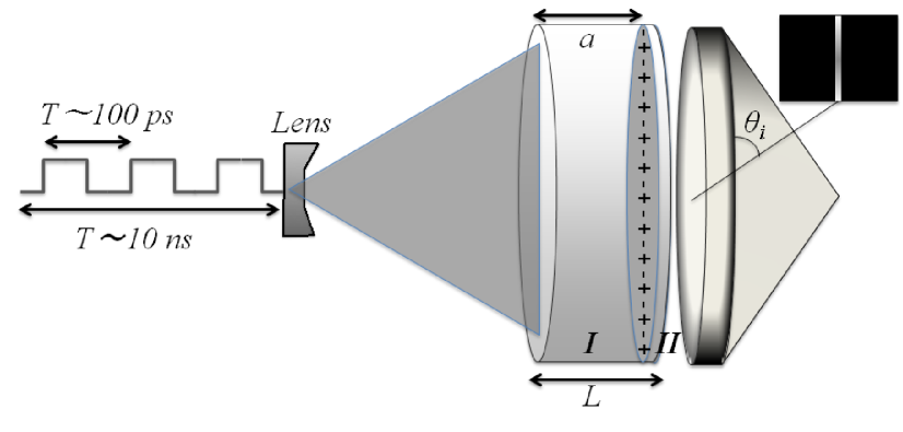
Figure 1: A pulse laser train of order $10-100$ pulses (repeating $\sim 10$ ms) uniformly irradiates (via a lens) a semiconductor/metal (SM) interface of radius $R$, composed of a dielectric of thickness $a$, region $I$ at a thin metal (e.g., silver) interface of thickness $(L-a)\ll L$, region $II$. Vacuum excited SPPs ($-\,+\,-\,+\,-\,+$) are detected using a phase matched prism placed to the right of region $II$.

II Theory

Our theoretical starting point is the following Lagrangian (from which Maxwell’s equations can be derived):

$${\cal L}=\frac{1}{2}\varepsilon(t)\left({\partial\over\partial t}\Phi\right)^{2}-\frac{1}{2}{1\over\mu(t)}(\nabla\Phi)^{2}-\frac{1}{2}m^{2}(t)\Phi^{2}$$ (1)

($\varepsilon_{0}=\mu_{0}=1$). In the above we assume that the electric permittivity and magnetic permeability are time dependent, but piecewise constant in space: $\nabla\mu=\nabla\varepsilon=0$. $\Phi$ represents a TM field with generalized Neumann BCs in a cavity and the TE case (swapping $\varepsilon\leftrightarrow\mu$) is represented by $\Psi$ with Dirichlet BCs, e.g., see Naylor (2012). This Lagrangian is useful because the standard canonical Hamiltonian can be constructed Kawakubo and Yamamoto (2011), where the mass term, $m^{2}(t)$, represents the coupling of light to a time-dependent boundary ($m^{2}$ can also arise from considering an electron plasma).

A convenient way to separate Maxwell’s equations is using Hertz vectors; developed by Nisbet Nisbet (1957) for non-dispersive inhomogeneous media. However, here we generalize to the case of a constant isotropic, but time-dependent medium. It is possible to show, see App. A, that Maxwell’s equations separate as

$$\varepsilon(t)\partial_{t}({\mu(t)\partial_{t}{\mathbf{\Pi}}_{e}})-\nabla^{2}{{\mathbf{\Pi}}_{e}} = 0~{},$$

$$\mu(t)\partial_{t}({\varepsilon(t)\partial_{t}{\mathbf{\Pi}}_{m}})-\nabla^{2}{{\mathbf{\Pi}}_{m}} = 0~{},$$ (2)

where we use a generalized Lorenz gauge (also discussed in App. A):

$$\mu(t)\partial_{t}(\varepsilon(t)A_{0})+\bm{\nabla}\cdot\mathbf{A}=0,$$ (3)

cf. Nisbet (1957); Bei and Liu (2011) and see Eq. (6). In the above we have assumed both a zero permanent polarization and magnetization ($\mathbf{P}_{0}=\mathbf{M}_{0}=0$) as well as zero bulk charges and currents ($\rho=0,\,\mathbf{J}=0$), although these can also be included in the Hertz method. Note the Lagrangian in Eq. (1) leads to the equations of motion for $\Pi_{e}$ in Eq. (2) ($\Pi_{m}$ is obtained by swapping $\mu\leftrightarrow\varepsilon$ in Eq. (1)), see App. A. This approach generalizes other work Uhlmann et al. (2004); Bei and Liu (2011) which considered only time-dependent $\varepsilon$ or $\mu$. Further work for non-dispersive, inhomogeneous, conducting and time-dependent media: $\varepsilon(\mathbf{r},t)$ and $\mu(\mathbf{r},t)$, will be presented elsewhere.

Before quantizing the SPP modes we first need to find the classical solutions for a single interface (between two media) that lead to SPPs. Writing the electric and magnetic fields in terms of Hertz vectors:

$${\mathbf{E}} = {1\over\varepsilon}\bm{\nabla}\times(\bm{\nabla}\times{\mathbf{\Pi}_{e}})-\mu_{0}\bm{\nabla}\times{\partial_{t}\mathbf{\Pi}_{m}}~{},$$

$${\mathbf{B}} = \mu\bm{\nabla}\times{\partial\mathbf{\Pi}_{e}\over\partial t}+\mu_{0}\bm{\nabla}\times(\bm{\nabla}\times{\mathbf{\Pi}_{m}})~{},$$ (4)

allowing one to easily isolate TE and TM modes, see App. B.

In what follows we take two half spaces in the $\hat{\mathbf{z}}$-direction, where region 1 (the semiconductor slab) is a semiconductor (I) and region 2 a metal (M) like silver, creating an SM interface. In our proposed set up $\varepsilon_{1}(t)$ varies from a minimum to maximum value and $\varepsilon_{2}<0$ remains constant (although for now it will be left more general). To make explicit the utility of the Hertz vector method we shall consider the radial propagation of SPPs in a cylindrical cavity with coordinates $(\rho,\theta,z)$, sectional radius $\rho=R$ and length $L$, see Fig. 1.

Using the Hertz potentials (2) and assuming from symmetry that $\mathbf{\Pi}_{m}=\Psi~{}\hat{\mathbf{z}}$ for TE, and $\mathbf{\Pi}_{e}=\Phi~{}\hat{\mathbf{z}}$ for TM modes, the separation of variables:

$$\Psi(\mathbf{x},t)=\sum_{\mathbf{l}}\psi_{\mathbf{l}}(\mathbf{x})q^{m}_{\mathbf{l}}(t)~{},$$

$$\Phi(\mathbf{x},t)=\sum_{\mathbf{l}}\phi_{\mathbf{l}}(\mathbf{x})q^{e}_{\mathbf{l}}(t)~{},$$ (5)

with $\mathbf{l}=(n,p,l)$, leads to the following wave equation, e.g., see Pedrosa and Rosas (2009):

$$\mathbf{\nabla}^{2}\psi_{\mathbf{l}}(\mathbf{x})+\varepsilon(t)\mu(t)\omega_{\mathbf{l}}^{2}(t)\psi_{\mathbf{l}}(\mathbf{x})=0~{}.$$ (6)

with the replacement $\psi_{\mathbf{l}}\to\phi_{\mathbf{l}}$ for TM modes. They satisfies the standard orthonormality conditions:

$$\int_{-\infty,0}^{\infty,L}d^{3}{\mathbf{x}}\,\psi_{\mathbf{l}}(\mathbf{x})\psi_{\mathbf{n}}(\mathbf{x})=(\psi_{\mathbf{l}},\psi_{\mathbf{n}})=\delta_{\mathbf{l}\mathbf{n}}$$ (7)

where the $(-\infty,\infty)$ bounds on the integral are for SPPs and that with $(0,L)$ are for the photon branch (see later). We then find that the time dependent part satisfies

$$\ddot{q}^{m}_{\mathbf{l}}+{\dot{\varepsilon}\over\varepsilon}\dot{q}^{m}_{\mathbf{l}}+\omega_{m\mathbf{l}}^{2}q^{m}_{\mathbf{l}}=0~{},$$ (8)

$$\ddot{q}^{e}_{\mathbf{l}}+{\dot{\mu}\over\mu}\dot{q}^{e}_{\mathbf{l}}+\omega_{e\mathbf{l}}^{2}q^{e}_{\mathbf{l}}=0~{}.$$ (9)

where the superscripts $m,e$ are for TE and TM modes respectively. Importantly, we see that for setups with only dielectrics present $\mu_{I,II}=$ constant then the TM mode functions are simple Mathieu like equations with natural frequency given by $\omega_{e\mathbf{l}}$. On the other hand for TE modes, the presence of $\dot{\varepsilon}$ and $\dot{q}_{m}$ leads to a detuning via $\tilde{\omega}_{m\mathbf{l}}$, see Eq. (37), and also losses for $\dot{\varepsilon}>0$ Pedrosa and Rosas (2009).

The conjugate momentum ${\cal P}_{m}=\partial{\cal L}/\partial t$ can be found from Eq. (1) along with the separation ansatz and orthonormality relations implying

$${\cal P}_{m}(\mathbf{x},t)=\varepsilon(t)\sum_{\mathbf{l}}\psi_{\mathbf{l}}(\mathbf{x})p^{m}_{\mathbf{l}}(t)$$ (10)

and via a Legendre transform we find the time dependent Hamiltonian for each mode $\mathbf{l}$ (TE):

$$H^{m}_{\mathbf{l}}=\varepsilon^{-1}{(p^{m}_{\mathbf{l}})^{2}\over 2}+{\varepsilon\over 2}\omega_{\mathbf{l}}^{2}(t)(q^{m}_{\mathbf{l}})^{2}$$ (11)

where the conjugate mode momentum is defined by

$$p^{m}_{\mathbf{l}}=\dot{q}^{m}_{\mathbf{l}}.$$ (12)

Given the ETCRs: $[\hat{q}_{\mathbf{l}},\hat{p}_{\mathbf{n}}]=i\delta_{\mathbf{l}\mathbf{n}}$, we get back the equation of motion, Eq. (8), from the above Hamiltonian. A similar analysis applies to TM modes: $\Phi,{\cal P}_{e}$ and hence we can quantize each degree of freedom $(\Phi,\Psi)$. In the above we rescaled the coordinates as $q^{m}_{\mathbf{l}}\to\varepsilon^{-1/2}q^{m}_{\mathbf{l}}$ for TE and would need $q^{e}_{\mathbf{l}}\to\mu^{-1/2}q^{e}_{\mathbf{l}}$ for TM modes (see later). In terms of these creation and annihilation operators we see squeezing terms in the Hamiltonian Pedrosa and Rosas (2009).

SPP and Photon Branches

To investigate SPPs for a single interface the ansatz:

$$\Phi_{\rm sp}(\mathbf{x},t)=\left\{\begin{array}[]{ccc}A_{1}e^{\kappa_{1l}(z-a)}r_{\rm np}(\mathbf{x}_{\bot})\,,&~{}z<a\,;~{}\varepsilon_{1},~{}\mu_{1}\,,\\ A_{2}e^{-\kappa_{2l}(z-a)}r_{\rm np}(\mathbf{x}_{\bot})\,,&~{}z>a\,;~{}\varepsilon_{2},~{}\mu_{2}\,,\end{array}\right.$$ (13)

leads to the following ‘time-dependent’ dispersion relations:

$$\mathbf{k}_{\bot}^{2}-\varepsilon_{1}\mu_{1}{\omega_{\mathbf{l}}^{2}\over c^{2}}=\kappa_{1l}^{2}\,,\qquad\mathbf{k}_{\bot}^{2}-\varepsilon_{2}\mu_{2}{\omega_{\mathbf{l}}^{2}\over c^{2}}=\kappa_{2l}^{2}$$ (14)

where Eq. (2) was used in each region. In cylindrical coordinates the transverse Laplacian is defined by

$$-\bm{\nabla}_{\bot}^{2}r_{\mathbf{k}_{\bot}}=\mathbf{k}_{\bot}^{2}r_{\mathbf{k}_{\bot}}$$ (15)

with eigenvalue $\mathbf{k}_{\bot}^{2}$. In DCE experiments the slab is usually bounded by a cavity (not depicted in Fig. 1) where

$$r_{\rm np}(\mathbf{x}_{\bot})={1\over\sqrt{\pi}}{1\over RJ_{n+1}(x_{\rm np})}J_{n}\Big{(}x_{\rm np}\frac{\rho}{R}\Big{)}e^{in\theta}~{},$$ (16)

$x_{\rm np}$ is the $p$th root of $J_{n}(x)=0$ Jackson (1998) and the fundamental cavity mode is $x_{01}=2.4048$. For a cavity bounding the SM interface in the transverse directions we would have $R_{sp}\leq R=2.5$ cm and hence $(\mathbf{k}^{\rm sp}_{\bot})^{2}=(x_{np}/R_{\rm sp})^{2}\sim{\cal O}(1)$, this depends on the value of $q$, cf. Eq. (32). For the photon branch we always have $(\mathbf{k}^{\rm ph}_{\bot})^{2}=(x_{np}/R)^{2}$ for a bounded cavity. Note in either case the mode functions are orthornormal: $(r_{\ell n},r_{np})=\delta_{\ell p}$.

Standard boundary conditions at an interface:

$$({\mathbf{D}}_{2}-{\mathbf{D}}_{1})\cdot{\hat{\mathbf{z}}}=0~{},\qquad{\hat{\mathbf{z}}}\times({\mathbf{E}}_{2}-{\mathbf{E}}_{1})=0$$ (17)

Jackson (1998) then imply $A_{1}=A_{2}$ and

$${\kappa_{1}(t)\over\varepsilon_{1}(t)}+{\kappa_{2}(t)\over\varepsilon_{2}(t)}=0$$ (18)

which requires that each dielectric be of opposite sign to generate SPPs Maier (2007). Eliminating the $z$-dependent $\kappa_{i}$ we then find the following ‘electric’ dispersion relation:

$$k_{\bot}=|\mathbf{k}_{\bot}|={\omega_{\bot}^{\rm sp}\over c}\sqrt{\varepsilon_{1}\varepsilon_{2}\over\varepsilon_{1}+\varepsilon_{2}}\times\left(\varepsilon_{1}\mu_{2}-\varepsilon_{2}\mu_{1}\over\varepsilon_{1}-\varepsilon_{2}\right)$$ (19)

With $\mu_{1}=\mu_{2}$ we get the standard result

$$(\omega_{\bot}^{\rm sp})^{2}={k_{\bot}^{2}c^{2}}\left({1\over\varepsilon_{1}}+{1\over\varepsilon_{2}}\right)~{},$$ (20)

where here we allow for time-dependent dielectrics, possibly in either region $I$ and $II$ and $\bot=(n,p)$ because for SPPs the axial direction $l$ is redundant. In Sec. III we will use a plasma-type model to obtain more detailed analytic properties of the above dispersion relation.

It is also worth mentioning that magnetic SPPs exist for TE modes Nesterenko and Pirozhenko (2012). Using the TE components of the Hertz vectors and using an equation like Eq. (13) for $\Psi(\mathbf{x},t)$ along with

$$({\mathbf{B}}_{2}-{\mathbf{B}}_{1})\cdot{\hat{\mathbf{z}}}=0~{},\qquad{\hat{\mathbf{z}}}\times({\mathbf{H}}_{2}-{\mathbf{H}}_{1})=0$$ (21)

lead again to $A_{1}=A_{2}$ but now with

$${\kappa_{1}(t)\over\mu_{1}(t)}+{\kappa_{2}(t)\over\mu_{2}(t)}=0.$$ (22)

As also discussed in Nesterenko and Pirozhenko (2012), SPPs can exist for TE modes as long as for example, $\mu_{1}<0,\,\mu_{2}>0$, which can be achieved using split ring resonators, e.g., see Maier (2007): using fabricated metamaterials. Finally using $\mathbf{\Pi}_{m}$ in Eq. (2) leads to the ‘magnetic’ dispersion relation:

$$k_{\bot}={\omega_{\bot}^{\rm sp}\over c}\sqrt{\mu_{1}\mu_{2}\over\mu_{1}+\mu_{2}}\times\left(\mu_{1}\varepsilon_{2}-\mu_{2}\varepsilon_{1}\over\mu_{1}-\mu_{2}\right)~{}.$$ (23)

This result can be obtained from the ‘electric’ sector by swapping $\varepsilon_{i}\leftrightarrow\mu_{i}$, and simplifies when $\varepsilon_{1}=\varepsilon_{2}$ to

$$(\omega_{\bot}^{\rm sp})^{2}={k_{\bot}^{2}c^{2}}\Big{(}{1\over\mu_{1}}+{1\over\mu_{2}}\Big{)}~{}.$$ (24)

As also discussed in Nesterenko and Pirozhenko (2012) this implies that TE modes can sustain surface plasmons; however, the material needs to be a fabricated metamaterial.

To compare vacuum excited SPPs with some experimental proposals for photon creation using semiconductor slabs, e.g., see Dodonov (2010), we will also consider TM modes in a slab of width $(L-a)$, placed in a cylindrical cavity of length $L$ (not shown). These have the following orthonormal mode functions for the TM photon Hertz scalar:

$$\Phi_{\rm ph}(\mathbf{r},t)=\left\{\begin{array}[]{ccc}A_{1}{\cos\,(k_{1l}z)}r_{\rm np}(\mathbf{x}_{\bot}),&0<z<a,\\ A_{2}\cos\,(k_{2l}(L-z))r_{\rm np}(\mathbf{x}_{\bot}),&a<z<L.\end{array}\right.$$ (25)

where (using the same TM interface conditions as before) we find following transcendental equation

$$\frac{k_{1l}\tan(k_{1l}a)}{\varepsilon_{1}(t)}=\frac{k_{2l}\tan(k_{2l}[a-L])}{\varepsilon_{2}(t)}$$ (26)

for the eigenvalues. This agrees with the result in Uhlmann et al. (2004) but can be derived with the minimum of effort using Hertz vectors and generalized to arbitrary transverse section. Note that the photon dispersion relation (in this case for a cylindrical section) at any given time in regions $i=1,2$:

$${\omega_{i\mathbf{l}}^{\rm ph}(t)}={c\over\varepsilon_{i}(t)}\sqrt{k_{il}^{2}(t)+\left(\frac{x_{\rm np}}{R}\right)^{2}}$$ (27)

must be equal at the interface implying equivalence of the dispersion relations:

$$\frac{1}{\varepsilon_{1}}\left(k_{1l}^{2}+\left(\frac{x_{\rm np}}{R}\right)^{2}\right)=\frac{1}{\varepsilon_{2}}\left(k_{2l}^{2}+\left(\frac{x_{\rm np}}{R}\right)^{2}\right).$$ (28)

Note this dispersion relation is the complex conjugate of that in Eq. (14): $k=i\kappa$. Both this constraint and the eigenvalue relation, Eq. (26), must be simultaneously satisfied Uhlmann et al. (2004). For slab thicknesses with $L-a\ll L$ (or for $a\ll L$) one can further show Uhlmann et al. (2004) that even for quite large variations in the dielectric constant the approximate solution to Eq. (26) is (for $l>0$)

$$k_{1l}(t)=\Big{(}{l\pi\over L}\Big{)}\Big{(}1-{a\over L}\Big{[}{\varepsilon_{1}(t)\over\varepsilon_{2}}-1\Big{]}\left(\frac{x_{\rm np}}{R}\right)^{2}\left(\frac{L}{l\pi}\right)^{2}\Big{)}~{}$$ (29)

(note TE modes at ${\cal O}(a/L)$ are still unperturbed free modes Uhlmann et al. (2004)).

Here we ignore the zero modes, $l=0$, as previous work Naylor (2012) for plasma sheets showed they are not excited; however, see discussion in Uhlmann (2004) for dielectrics. In this case the interface constraint, Eq. (28), suggests that $k_{i0}=0$ ($i=1,2$) implies $\varepsilon_{1}=\varepsilon_{2}$ and is therefore only satisfied for time independent (static) cases. The general case, not just for $\eta=a/L\ll 1$, will be investigated more thoroughly elsewhere. We therefore assume the TM₀₁₁ is the lowest mode and investigate the number of created particles for this and the TE₁₁₁ fundamental mode (up to ${\cal O}(a/L)$), comparing them to that for SPPs.

III Generalized Plasma Model

Region $II$: Time Independent

To simplify our analysis we will now consider a slight generalization of the plasma model Kawakubo and Yamamoto (2011) of a metal-like substance in region $II$:

$$\varepsilon_{2}(\omega)=\bar{\varepsilon}_{2}\left(1-\left({\omega_{p}^{2}\over\omega^{2}}\right)\right)$$ (30)

where $\omega_{p}=ne^{2}/(\bar{\varepsilon}_{2}m_{*})$ is the plasma frequency and $n$ is the number of bulk electrons and $m_{*}$ is the effective mass. The extra multiplicative factor arises by including a mass term in the Lagrangian, Eq. (1). In our envisaged experiment $\bar{\varepsilon}_{2}$ will be a constant, but for generality we have left it time dependent, $\bar{\varepsilon}_{2}(t)$, in the analysis below. Note the dielectric permittivity in region $II$ takes negative values for $\omega<\omega_{p}$. For region $I$ we assume a semiconductor material that is modulated by laser irradiation.

If we then substitute Eq (30) into Eq. (20) (using $\omega=\omega_{\bot}^{\rm sp}$) we obtain a generalization of the solution found in Nesterenko and Pirozhenko (2012):

$$(\omega_{\bot}^{\rm sp})^{2} = \omega_{p}^{2}\left[\frac{1}{2}+\frac{1}{2}q^{2}\left({1\over\varepsilon_{1}}+{1\over\bar{\varepsilon}_{2}}\right)\right.$$

$$-\left.\sqrt{\frac{1}{4}+\frac{1}{4}q^{4}\left({1\over\varepsilon_{1}}+{1\over\bar{\varepsilon}_{2}}\right)^{2}+\frac{1}{2}q^{2}\left({1\over\bar{\varepsilon}_{2}}-{1\over\varepsilon_{1}}\right)}\right]$$

where

$$q={k_{\bot}c\over\omega_{p}}$$ (32)

and we obtain the standard result for $\bar{\varepsilon}_{1}=\varepsilon_{2}=1$ Nesterenko and Pirozhenko (2012).

We also find the following asymptotic behavior:

$$\omega_{\bot}^{\rm sp}\to{k_{\bot}c}\left({1\over\varepsilon_{2}}\right)^{1/2}+{\cal O}(q^{3})+\dots \quad q\to 0,$$

$$\omega_{\bot}^{\rm sp}\to{\omega_{p}\over\sqrt{2}}+{\cal O}(q^{-2})+\dots \quad q\to\infty~{},$$

which explains why for small $q$, we have a system that behaves like TE/TM modes in a 1D cavity. Hence for a given form of modulation (see below) of the dielectric, the limit $q\to 0$ leads to parametric amplification of SPPs; while $q\to\infty$ gives no SPP production (for $\omega_{p}=$ constant).

Region $I$: Time Dependence

To be more specific, in this paper we will consider two kinds of modulation of the dielectric in region $I$, given that in Eq (30) for region $II$.

One, an inverse sinusoidal modulation:

$${1\over\varepsilon_{1}}=\frac{1}{2}\Big{(}{1\over\varepsilon_{\rm 1,min}}+{1\over\varepsilon_{\rm 1,max}}\Big{)}+\frac{1}{2}\Big{(}{1\over\varepsilon_{\rm 1,min}}-{1\over\varepsilon_{\rm 1,max}}\Big{)}\cos(2\omega_{0}t)$$ (34)

that has been argued to arise from the excitation of localized electrons in a semiconductor, via laser irradiation (e.g., see Uhlmann (2004)). In this regard, we should mention that for the excitation of electrons to the conduction band, instead of using a dielectric model, such as Eq. (34), the conductivity modulates by assuming the plasma frequency varies with, for example, a sin-like time dependence: $\omega_{p}(t)=e^{2}n(t)/m_{*}$, where $n_{s}(t)\propto\sin(2\omega_{0}t)$, and an equation like that in Eq. (30) but instead for region $I$. This is an interesting problem but differs in that $\varepsilon_{1}<0$ for certain modulations and will be left for future work (also see Naylor (2012) for more on plasma sheet models). In this article we will assume that $\varepsilon_{1,min},\varepsilon_{1,max}>0$.

Another way to realistically modulate the permittivity, $\varepsilon_{1}(t)$, but this time sinusoidally would be to use an appropriately doped semiconductor (with two well defined energy levels within the band gap) via Rabi oscillations, e.g, see Haug and Koch (2004):

$${\varepsilon_{1}}=\frac{1}{2}\Big{(}{\varepsilon_{\rm 1,max}}+{\varepsilon_{\rm 1,min}}\Big{)}+\frac{1}{2}\Big{(}{\varepsilon_{\rm 1,max}}-{\varepsilon_{\rm 1,min}}\Big{)}\cos(2\omega_{0}t)$$ (35)

In the next section we shall assume that for both cases we have $\varepsilon_{1,min}=0.2$ and $\varepsilon_{1,max}=3.2$ which are typical values for a germanium semiconductor.

IV Particle Creation Rates

To find the number of particles created we use an alternative to the Bogoliubov method using only mode functions Kofman et al. (1997). We start with the quantum field operator expansion in the Heisenberg representation for our TM Hertz potential:

$$\hat{\Phi}({\bf x},t)=\sum_{l}\left[\hat{a}_{\mathbf{l}}\varphi_{l}(\mathbf{x})q_{l}(t)+\hat{a}_{l}^{\dagger}\varphi^{*}_{l}(\mathbf{x})q^{*}_{l}(t)\right]~{},$$ (36)

where $\hat{a}_{l},\hat{a}_{l}^{\dagger}$ are annihilation and creation operators respectively and the mode functions $\varphi_{\mathbf{l}}(\mathbf{x}),~{}q_{\mathbf{l}}(t)$ were defined in Eqs. (6,7,8); here we need to impose initial conditions at $t=0$: $q_{l}(0)={1\over\sqrt{2\tilde{\omega}_{l}}}$ and $\dot{q}_{l}(0)=-i\sqrt{\tilde{\omega}_{l}\over 2}$. To find a separable time-dependent solution we can rescale the field as $\tilde{q}_{\mathbf{l}}=\varepsilon^{1/2}q_{\mathbf{l}}$ to get an equation in Mathieu form:

$$\ddot{\tilde{q}}_{l}+\tilde{\omega}_{l}^{2}(t)\tilde{q}_{l}=0~{}.$$ (37)

where

$$\tilde{\omega}_{l}^{2}=\left[\omega_{l}^{2}+\frac{1}{4}{\dot{\varepsilon}^{2}\over\varepsilon^{2}}-\frac{1}{2}{\ddot{\varepsilon}\over\varepsilon}\right]~{}.$$ (38)

It may be worth mentioning that this equation is equivalent to a scalar potential in a curved spacetime with conformal coupling $\xi=1/6$ and scale factor $\varepsilon(t)=a(t)$ for a Robertson-Walker spacetime Birrell and Davies (1982).

The particle number density can be obtained directly from the energy of each mode divided by the energy $\omega_{l}$ of each particle:

$$n_{l}={\tilde{\omega}_{l}\over 2}\left({|\dot{\tilde{q}}_{l}|^{2}\over\tilde{\omega}_{l}^{2}}+|\tilde{q}_{l}|^{2}\right)-\frac{1}{2}$$ (39)

where we have subtracted off the zero point energy with units $\hbar,c=1$. Eq. (37) has a well known structure of narrow or broad resonances for certain parameters. We stress that this method has separated variables without using an instantaneous basis approximation (see App. C).

Before numerically solving for the number of created particles, we will estimate the pair creation rate analytically. If the background field (the laser) leads to shifts in frequency near to parametric resonance:

$$\omega_{\mathbf{m}}^{2}(t)\sim\omega_{0\mathbf{m}}^{2}+\Delta\omega_{0\mathbf{l}}^{2}=\omega_{0\mathbf{m}}^{2}(1+\kappa\cos(\Omega_{\mathbf{l}}t)),$$ (40)

where the driving frequency is chosen as $\Omega_{\mathbf{m}}=2\omega_{0\mathbf{m}}$, where ${\mathbf{m}}=(\bot,{\mathbf{l}})$, for SPPs or photons respectively, then in the late time limit:

$$n_{\mathbf{m}}\approx\sinh^{2}\left({\omega_{0\mathbf{m}}\kappa t/4}\right),$$ (41)

which can be derived by ignoring second order time derivatives in Eq. (37) Dodonov et al. (1993).

As a simple example consider $\mu_{1}=\mu_{2}$, where the time-dependent ‘electric’ SPP dispersion relation, Eq. (LABEL:plasmadis), could be varied using a laser with driving frequency, $\Omega_{l}=2\omega_{0l}$ for $\bar{\varepsilon}_{2}>0$ and constant, cf. Eq. 30, with $\varepsilon_{1}$ varying inverse sinusoidally as $\varepsilon_{\rm min}<\varepsilon_{1}(t)<\varepsilon_{\rm max}$ then

$${\varepsilon_{2}\over\varepsilon_{1}(t)}\sim\chi+\kappa\cos(2\omega_{0l}t),$$ (42)

where $\chi>0$ is an overall time-independent frequency shift (cf. Eq (34). Then Eq. (41) leads to a particle rate:

$$n_{\bot}^{\rm sp}=\sinh^{2}\left(k_{\bot}^{2}c^{2}{\kappa\over 4\varepsilon_{2}}t\right)~{}.$$ (43)

This equation is also valid for the more general case of $\varepsilon_{2}<0$ not just the model discussed in Sec. III.

We can now compare this to the $\omega_{011}$ TM mode (the lowest frequency cylindrical mode Naylor (2012)) where in the limit of $(L-a)\ll L$, from Eq. (29) and equivalence of the dispersion relations (see below Eq. (27)), the photon eigenvalues shift by (to order ${\cal O}(a/L)$):

$$\Delta\omega_{0\mathbf{l}}^{2}(t)=\frac{2x_{np}^{2}c^{2}}{R^{2}\varepsilon_{2}}\frac{a}{L}\left[\frac{\varepsilon_{2}}{\varepsilon_{1}(t)}-1\right].$$ (44)

Parametric enhancement for the photon branch is then achieved by choosing

$${\varepsilon_{2}\over\varepsilon_{1}(t)}\sim\chi+\kappa\cos(2\omega_{0l}t)~{},$$ (45)

where for photons $\chi$ and $\kappa$ may or may not be the same as those for SPPs; however they are assumed of the same magnitude. Note the resonant frequencies are not the same: $\omega_{0\bot}\neq\omega_{0\mathbf{l}}$. This leads to:

$$n_{\mathbf{l}}^{\rm ph}=\sinh^{2}\left({x_{np}^{2}c^{2}\over R^{2}}{a\kappa\over 2\varepsilon_{2}L}t\right).$$ (46)

Thus, for a cylindrical cavity the SPP creation rate dominates the photon rate if $k_{\bot}^{2}\gg(x_{np}^{2}/R^{2})(2a/L)$. For example, with a cavity of radius, $R=2.5$, cm and length, $L=10$ cm, then for $a/L\sim{\cal O}[10^{-4}]$ and $x_{01}=2.4048$ we require that $k_{\bot}^{2}\gg 1/25$, or $k_{\bot}\gg 1/5$. This is easily achieved for SPPs which have their modes bounded by a transverse section.

We have also confirmed these findings numerically by assuming both an inverse sinusoidal, cf. Eq. (34), and a sinusoidal variation, cf. Eq. (35), for region $I$, see upper and lower panels in Fig. 2, respectively. In both examples we have assumed $\varepsilon_{1,max}=3.2$ to $\varepsilon_{1,min}=0.2$ where as we mentioned the inverse profile is meant to model the laser irradiation of a doped semiconductor, while the latter one models the Rabi like oscillations in a pure semiconductor Uhlmann (2004). Here we chose the transverse radial section for the dielectric slab and SPPs to be $R_{\rm sp}=R=2.5$ cm, the slab radius (used in $k_{\bot}=x_{\rm np}/R$). It may be worth mentioning that for $q=(k_{\bot}c/\omega_{p})\to 0$ (Zenneck waves) the propagation length becomes unbounded, but by enclosing the SM interface within a cavity of transverse section, $k_{\bot}$ stays bounded.

In Fig. 3 we also plotted the creation rate numerically for the fundamental TE₁₁₁ cylindrical mode, for a sinusoidal variation. We see that the SPP rate is of a similar magnitude for both inverse sinusoidal & sinusoidal variations and we also see that both TM branch SPP and photons are a magnitude larger when compared to sinusoidal ones. This indicates that using doped-semiconductors would lead to easier detection of pair created photons or vacuum SPPs, although a priori we should consider the effects of dissipation and solve the photon eigenvalues, Eq. (26), for general values of $\eta=a/L$ (see Sec. VI).

V Detection Scheme

In our proposed detection scheme, see Fig. 1, we have chosen region $II$ to be that of a metal such as silver and hence satisfies $\varepsilon_{2}<0$ for frequencies blow the plasma frequency, $\omega_{p}$, cf. Eq. (30). To realistically modulate the permittivity, $\varepsilon_{1}(t)$, we have discussed possible inverse and sinusoidal variations arising from the excitation of localized electrons below the conductions band Uhlmann (2004) and arising from intra-band transitions in a doped semiconductor, Haug and Koch (2004), respectively. As we mentioned, for laser pulses with an energy ($h\lambda/c$) above the band gap, a time varying bulk conductivity, $\rho(t)$, would be generated leading to a modulated permittivity with $\varepsilon_{\rm min}<0$ (shifts $\chi<0$) and will be left for future investigation. Hence, in this article we only consider SM interfaces such that one interface region $I$ has $\varepsilon_{1}(t)>0$, and the other region $II$ always has $\varepsilon_{2}<0$.

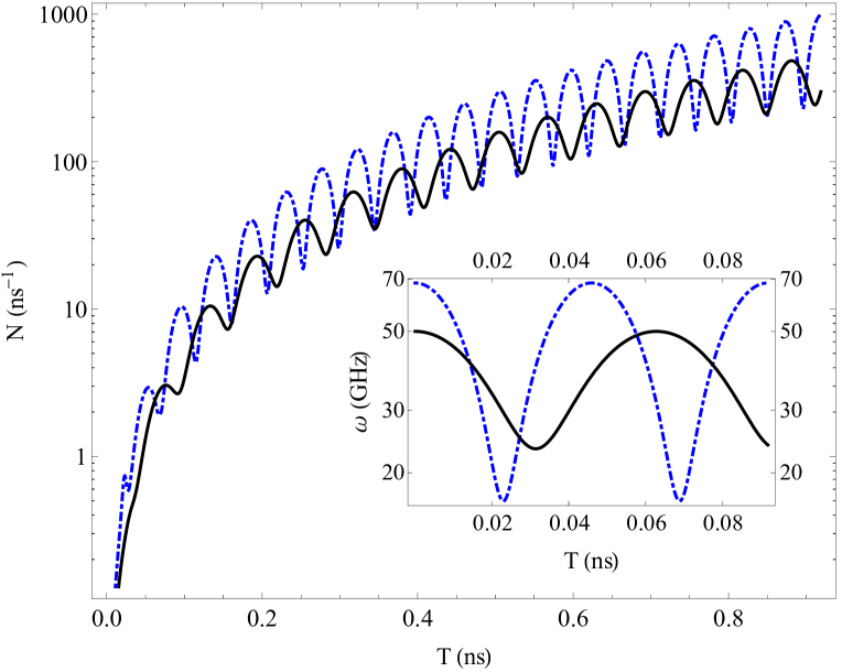
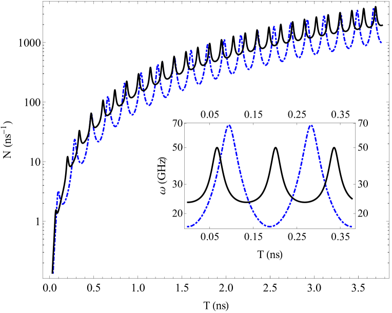
Figure 2: (Color online) Particle creation rates for SPPs (solid-dark) and 2nd fundamental TM₀₁₁ (dot-dashed-blue), for a pulse train of $~{}100$ pulses, $\eta=0.01$, $R_{\rm sp}=R=2.5$ cm, region $II$ with $\bar{\varepsilon}_{2}=1.0$ and $\omega_{p}=1.5\times 10^{15}$ s^-1 for silver. In region $I$ we have: a) an inverse sinusoidal variation (upper panel) and b) a sinusoidal variation (lower panel) ranging from $\varepsilon_{1,max}=3.2$ to $\varepsilon_{1,min}=0.2$ (see Eq. (34, 35)). Insets: Plots $\omega_{\mathbf{l}}^{\rm spp}$, $\omega_{011}^{\rm phot}$ for each case.

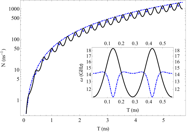
Figure 3: (Color online) Comparison with Fig. 2 (lower panel) for TE modes. The particle creation rate for single mode coupling in the instantaneous basis approximation (solid-dark) and the exact solution (dot-dashed-blue) for a sinusoidal variation. cf. Eq. (35), for TE₁₁₁ with the same conditions as in Fig. 2. Inset: Comparison of $\tilde{\omega}_{111}^{\rm phot}$ and $\omega_{111}^{\rm phot}$.

One possible way to detect vacuum excited SPPs would be to use near-field microscopy with a photon scanning tunneling microscope, e.g., see Maier (2007), where the microscope is placed on the opposite vacuum or air side of the SM interface: region $II$, see Fig. 1. Usually, to generate SPPs a monochromatic light source is sent into a prism placed above the interface with total internal reflection at angle $\theta_{i}$. The SPPs are detected by finding a decrease in emitted power at $\theta_{i}$. However, the time reversed case is equivalent to the creation of vacuum excited SPPs and therefore would lead to a telltale signature: SPPs would be created via the observation of an increase in emitted power at $\theta_{i}$ during the time modulation of $\varepsilon_{1}$. We should; however, require that the pulsed laser itself does not generate SPPs, as can be arranged by uniformly irradiating the dielectric slab at 90 degrees incidence, see Fig. 1.

The experimental details we mentioned so far are simple extensions of current DCE experiments Agnesi et al. (2009). However, it may well also be possible to use experiments that have already detected DCE analog radiation in metamaterials Lähteenmäki et al. (2013). The analogy of SPPs in this work with metamaterials comes from considering flux qubits coupled to coplanar waveguides Paraoanu (2010). Such experimental conditions have already been demonstrated Astafiev et al. (2010) by coupling artificial atoms to carbon nanotubes and it seems within reach of current technology to also adapt these experiments to time-dependent variations of flux qubits (already done in Wilson et al. (2011); Lähteenmäki et al. (2013) for photon analogs).

We can also go further with metamaterials, where say $\mu_{2}<0$ where in the late time limit the SPP creation rate is:

$$n_{\bot}^{\rm sp}=\sinh^{2}\left({k_{\bot}^{2}c^{2}}{\kappa\over 4\mu_{2}}t\right)$$ (47)

for

$${\mu_{2}\over\mu_{1}(t)}\sim\chi+\kappa\cos(2\omega_{0l}t).$$ (48)

Given that $\sinh(-x)=-\sinh x$ there is no problem in having $\mu_{2}<0$ because $n_{\bot}^{\rm sp}$ depends quadratically on $\sinh$.

This rate is also comparable to the photon-photon rate if $\mu_{1}$ were varied in time above GHz frequencies. It would be interesting to try and design experiments in centimeter/micrometer sized cavities using split ring resonators and wire rods that are then modulated in time. This leads to easier detection by precisely controlling the SPP wavelength, $\lambda_{\rm sp}$.

VI Conclusion & Outlook

We have discussed how SPPs can be excited out of the vacuum for the case where a dielectric crystal changes from a minimum to maximum value at a semiconductor semispace/metal (SM) interface during laser irradiation. We separated Maxwell’s equations in a generalized Lorenz gauge for time-dependent media, both for the permittivity and permeability. For parametric oscillations of a dielectric slab our analytic and numerical analyses show that vacuum excited SPPs can be of the same order of magnitude as the photon-photon rate.

The results for the photon creation rate in a cylindrical cavity (generalizing the rectangular case Uhlmann et al. (2004)) were also found. For experimental proposals to detect DCE radiation Agnesi et al. (2009), the detection of vacuum excited SPPs has added benefits as compared to photon modes: SPPs do not actually need a bounding cavity as they are planar modes (only photon modes need this for parametric enhancement) and for $\mu_{i}=$ constant, TM branch SPP and photon modes are not detuned from their resonant frequencies like TE photons.

As future work we should also include dissipative effects, because even without ${\rm Im}[\varepsilon]\neq 0$, it is possible to have imaginary $\tilde{\omega}$ the photon branch. The separation of variables method used here Pedrosa and Rosas (2009) that we generalized to a Lorenz-like gauge, naturally allows one to incorporate ${\rm Im}[\varepsilon]$. In fact, for ${\rm Im}[\varepsilon]$, the propagation length via $(2{\rm Im}[k_{\bot}])^{-1}$ for SPPs diminishes, not the production rate, so this might lead to another benefit. These and other issues including de-tuning of resonant frequencies arising from dissipation will be addressed elsewhere.

It would also be interesting to investigate the vacuum excitation of volume/bulk plasmon polaritons (VPPs), usually created by firing a beam of electrons, e.g., see Raether (1988), because longitudinal modes are not excited by light and hence require particle impact at an interface, e.g., see Maier (2007). However, vacuum excitations might be achieved dynamically by firing clusters of ‘neutral’ Argon atoms at a sample of material Inui et al. (2008), or by placing the sample on a high frequency piezo, e.g., see Kim et al. (2006). The issue of the gap between bulk and surface plasmons Raether (1988) indicates they are more difficult to create.

Finally, for time dependent media, it has recently been suggested Bei and Liu (2011) that not only transverse (TE and TM) modes, but also longitudinal modes can be created out of vacuum. These are usually unphysical in Gupta-Bleuler quantization due to a cancellation among time and longitudinal components. However the authors in Bei and Liu (2011) argue that for a time-dependent permittivity: $\varepsilon(t)$, such a cancellation does not occur and surface charges arise as a real physical effect from longitudinal modes. The issue of quantization in general time dependent media requires further investigation, where it would be interesting to find the relationship, or difference, between vacuum excited SPPs and possible surface charges from longitudinal modes.

Note Added— While this work was under revision, a paper dealing with the spontaneous emission of photon pairs from a metamaterial junction Ghosh and Maiti (2013) appeared in the literature. However, we consider instead the stimulated emission of photon pairs from non-adiabatic changes in the vacuum state. We also came across work with similar ideas to those given here: that surface plasmons can be created out of vacuum excitations at a time modulated interface Hizhnyakov et al. (2015).

Appendix A Time dependent backgrounds

Here we discuss a convenient way to separate Maxwell’s equations using Hertz vectors. This was developed by Nisbet Nisbet (1957) for non-dispersive inhomogeneous time-dependent media. Here we generalize to the case of an isotropic and time-dependent medium.

Maxwell’s equations in SI units are:

$$\bm{\nabla}\cdot\mathbf{B}=0,\qquad\qquad\bm{\nabla}\times\mathbf{E}=-\dot{\mathbf{B}}$$

$$\bm{\nabla}\cdot\mathbf{D}=\rho,\qquad\qquad\bm{\nabla}\times\mathbf{H}-\dot{\mathbf{D}}=\mathbf{J}$$ (1)

where

$$\mathbf{D}=\varepsilon(t,\mathbf{x})\mathbf{E}\qquad\qquad\mathbf{B}=\mu(t,\mathbf{x})\mathbf{H}$$ (2)

In the above we have assumed both a zero permanent polarization and magnetization ($\mathbf{P}_{0}=\mathbf{M}_{0}=0$) and later we will also assume zero bulk charges and currents ($\rho=0,\,\mathbf{J}=0$), although for now we keep them to see how general Maxwell’s equations can remain in order to separate them.

We now define the electromagnetic fields in terms of gauge potentials as follows:

$$\mathbf{B}=\bm{\nabla}\times\mathbf{A}~{}\qquad\qquad\mathbf{E}=-\partial_{t}\mathbf{A}-\bm{\nabla}A_{0}$$ (3)

where upon substitution into Maxwell’s equations (1) we find that Gauss’ and Ampere’s laws lead to:

$$-\bm{\nabla}\cdot\Big{(}\varepsilon{\partial\over\partial t}\mathbf{A}\Big{)}-\bm{\nabla}\cdot\Big{(}\varepsilon\bm{\nabla}A_{0}\Big{)} = \mathbf{\rho},$$

$${\partial\over\partial t}\Big{(}{\varepsilon{\partial\over\partial t}\mathbf{A}}\Big{)}+{\partial\over\partial t}\Big{(}\varepsilon\bm{\nabla}A_{0}\Big{)}+\bm{\nabla}\times\Big{(}{1\over\mu}\bm{\nabla}\times\mathbf{A}\Big{)} = \mathbf{J}.$$

At this point separation of these coupled equations requires some assumptions to be made. The separation in the Coulomb gauge was achieved in the seminal paper by Dodonov, Klimov and Nikonov Dodonov et al. (1993) assuming a factorisable ansatz: $\varepsilon(\mathbf{r},t)=\varepsilon(t)\varepsilon(\mathbf{x})$ and $\mu(\mathbf{r},t)=\mu(t)\mu(\mathbf{x})$.

The separation is more difficult in the Lorenz gauge; however, Nisbet Nisbet (1957) was able to separate Maxwell’s equations using what we shall call a generalized spatial Lorenz gauge:

$$\mu\varepsilon\partial_{t}(A_{0})+\bm{\nabla}\cdot(\varepsilon(\mathbf{x})\mathbf{A})=0,$$ (5)

assuming time-independent media, which is not the standard Lorenz gauge. For the case of time-dependent media, a generalized temporal Lorenz gauge can be found:

$$\mu(t)\partial_{t}(\varepsilon(t)A_{0})+\bm{\nabla}\cdot\mathbf{A}=0,$$ (6)

which works as long as we assume an isotropic piecewise homogeneous and time dependent media: $\varepsilon(t),\mu(t)$ and $\nabla\mu=\nabla\varepsilon=0$, cf. Bei and Liu (2011) for the case of $\mu=1$. Note a generalized spatio-temporal Lorenz gauge of the form $\mu(t)\partial_{t}(\varepsilon(t)A_{0})+\bm{\nabla}\cdot(\varepsilon(\mathbf{x})\mathbf{A})$ does not lead to a complete separation as can be verified. However, the separation of a non-dispersive, inhomogenous, conducting and time-dependent medium assuming a factorisable geometry (cf. Dodonov et al. (1993)) appears to be possible and will be presented elsewhere.

Plugging in the temporal Lorenz gauge, Eq. (6), into Eq. (A), assuming $\nabla\varepsilon=\nabla\mu=0$, leads to two uncoupled second order differential equations of the form

$${\partial\over\partial t}\Big{(}\mu{\partial\over\partial t}(\varepsilon A_{0})\Big{)}-\nabla^{2}A_{0} = {\rho\over\varepsilon}$$

$$\mu{\partial\over\partial t}\Big{(}\varepsilon{\partial\over\partial t}\mathbf{A}\Big{)}-\nabla^{2}\mathbf{A} = \mathbf{\mu}\mathbf{J}~{},$$ (7)

which generalizes the result found in Bei and Liu (2011) when $\mu=1$. The above result also generalizes work in the Coulomb gauge by Dodonov et al. Dodonov et al. (1993) and work in Uhlmann et al. (2004) which considered either time-dependent $\varepsilon$, or $\mu$ using dual potentials and hence does not allow for the inclusion of charge and current densities which break the duality Jackson (1998) (also see Pedrosa and Rosas (2009) for time-dependent media in the Coulomb gauge).

Note the two equations (7) are not symmetric in an interchange of $\varepsilon\leftrightarrow\mu$ which is due to the non-trivial time-dependence of the media. However, a symmetric set of equations (with respect to $\varepsilon\leftrightarrow\mu$) can be obtained from the Hertz method as we show in the next section.

Appendix B Hertz Vectors

We now define two Hertz vectors $\mathbf{\Pi}_{e}$ and $\mathbf{\Pi}_{m}$ as (with $\mu_{0}=1$)

$$A_{0}=-{1\over\varepsilon}\bm{\nabla}\cdot\mathbf{\Pi}_{e},\quad{\mathbf{A}}=\mu{\partial\mathbf{\Pi}_{e}\over\partial t}+\bm{\nabla}\times{\mathbf{\Pi}_{m}}$$ (8)

which automatically satisfies the temporal Lorenz gauge condition, Eq. (6), see Nisbet (1957) for the definition of potentials on a spatial Lorenz gauge. It is then possible to show that the coupled wave equation, Eq. (7), separates as:

$$\varepsilon(t)\partial_{t}({\mu(t)\partial_{t}{\mathbf{\Pi}}_{e}})-\nabla^{2}{{\mathbf{\Pi}}_{e}} = \mathbf{Q}_{e}$$

$$\mu(t)\partial_{t}({\varepsilon(t)\partial_{t}{\mathbf{\Pi}}_{m}})-\nabla^{2}{{\mathbf{\Pi}}_{m}} = \mathbf{Q}_{m}~{},$$ (9)

where TE modes correspond to $\mathbf{\Pi}_{m}$ while TM modes are those for $\mathbf{\Pi}_{e}$ (for more details see below Eq. (2)). Here we have included the so-caled “stream potentials” Nisbet (1957):

$$\mathbf{\nabla}\cdot\mathbf{Q}_{e}=-\rho$$

$$\dot{\mathbf{Q}}_{e}+{1\over\mu}\mathbf{\nabla}\times\mathbf{Q}_{m}=\mathbf{J}$$ (10)

set to zero in the main text as we assume that $\rho,\mathbf{J}=0$, cf. Eq. (2). It may also be worth mentioning that these equations are slightly different to the case discussed in Nesterenko and Pirozhenko (2012) that applies to a dispersive medium: $\varepsilon(\omega),\mu(\omega)$, on a time-independent ($e^{i\omega t}$) background.

The electric and magnetic fields can then be written in terms of Hertz vectors as

$${\mathbf{E}} = {1\over\varepsilon}\bm{\nabla}(\bm{\nabla}\cdot\mathbf{\Pi}_{e})-\partial_{t}(\mu\,\partial_{t}\mathbf{\Pi}_{e})-\bm{\nabla}\times{\partial_{t}\mathbf{\Pi}_{m}}$$

$$= {1\over\varepsilon}\bm{\nabla}\times(\bm{\nabla}\times{\mathbf{\Pi}_{e}})-\bm{\nabla}\times{\partial_{t}\mathbf{\Pi}_{m}}~{},$$

$${\mathbf{B}} = \mu\bm{\nabla}\times{\partial\mathbf{\Pi}_{e}\over\partial t}+\bm{\nabla}\times(\bm{\nabla}\times{\mathbf{\Pi}_{m}})~{},$$ (11)

allowing one to easily isolate TE and TM modes.

For example, TM modes are defined by the parts $\mathbf{E}_{TM},\mathbf{B}_{TM}$ coming from $\mathbf{\Pi}_{e}$ with $\mathbf{z}\cdot\mathbf{B}=0$, where a convenient choice of Hertz vectors are:

$${\mathbf{\Pi}}_{e}=\Phi\,\hat{\mathbf{z}}\,,\qquad{\mathbf{\Pi}}_{m}=\Psi\,\hat{\mathbf{z}}$$

and $\Phi$ and $\Psi$ represent TM and TE modes respectively. For TM modes we obtain

$${\mathbf{E}}_{TM} = {1\over\varepsilon}\partial_{1}\partial_{z}\Phi\hat{\mathbf{e}}_{1}+{1\over\varepsilon}\partial_{2}\partial_{z}\Phi\hat{\mathbf{e}}_{2}~{},$$

$$\ {\mathbf{B}}_{TM} = \mu\,\partial_{2}\partial_{t}\Phi\hat{\mathbf{e}}_{1}-\mu\,\partial_{1}\partial_{t}\Phi\hat{\mathbf{e}}_{2}$$ (12)

with a similar expression for TE modes (from $\mathbf{\Pi}_{m}$ with $\mathbf{z}\cdot\mathbf{E}=0$):

$${\mathbf{E}}_{TE} = -\partial_{2}\partial_{t}\Psi\hat{\mathbf{e}}_{1}+\partial_{1}\partial_{t}\Psi\hat{\mathbf{e}}_{2}~{},$$

$$\ {\mathbf{B}}_{TE} = \partial_{1}\partial_{z}\Psi\hat{\mathbf{e}}_{1}+\partial_{2}\partial_{z}\Psi\hat{\mathbf{e}}_{2}~{}.$$ (13)

These generalize the time-independent cases found e.g. in Nesterenko and Pirozhenko (2012).

These equations of course combine for both TE and TM modes to give the total electric and magnetic field strengths:

$${\mathbf{E}} = \left({1\over\varepsilon}\partial_{1}\partial_{z}\Phi-\partial_{2}\partial_{t}\Psi\right)\hat{\mathbf{e}}_{1}+\left({1\over\varepsilon}\partial_{2}\partial_{z}\Phi+\partial_{1}\partial_{t}\Psi\right)\hat{\mathbf{e}}_{2}-{1\over\varepsilon}\bm{\nabla}_{\bot}^{2}\Phi\,\hat{\mathbf{z}}$$ (14)

$${\mathbf{B}} = \left(\mu\,\partial_{2}\partial_{t}\Phi+\partial_{1}\partial_{z}\Psi\right)\hat{\mathbf{e}}_{1}+\left(-\mu\,\partial_{1}\partial_{t}\Phi+\partial_{2}\partial_{z}\Psi\right)\hat{\mathbf{e}}_{2}-\bm{\nabla}_{\bot}^{2}\Psi\,\hat{\mathbf{z}}$$

and generalizes the time-independent case, e.g., see Nesterenko and Pirozhenko (2012), to the time-dependent case.

Appendix C Separation of variables in time-dependent media

To allow for space-time-dependent mode functions we can also use an instantaneous basis Law (1994):

$$\Phi(\mathbf{r},t)=\sum_{m}Q_{\mathbf{m}}(t)\varphi_{\mathbf{m}}(\mathbf{r};t)~{},$$ (15)

where now $t$ becomes a parameter: $\varphi(\mathbf{r},t)\to\varphi(\mathbf{r};t)$. The orthonormality again is given by

$$\int_{0}^{L}dz\,\varepsilon(t)\varphi_{\mathbf{m}}(\mathbf{r};t)\varphi_{\mathbf{n}}(\mathbf{r};t)=(\varphi_{\mathbf{m}},\varphi_{\mathbf{n}})=\delta_{\mathbf{m}\mathbf{n}}$$ (16)

and satisfies the wave equation:

$$\mathbf{\nabla}^{2}\varphi_{\mathbf{m}}(\mathbf{r};t)+\varepsilon(t)\mu(t)\omega_{\mathbf{m}}^{2}(t)\varphi_{\mathbf{m}}(\mathbf{r};t)=0.$$ (17)

These steps appear to be identical to the standard separation of variables; however the time dependent wave equation now becomes Law (1994), cf. Eq. (8):

$$\ddot{Q}_{\mathbf{m}}+\omega_{\mathbf{m}}^{2}(t)Q_{\mathbf{m}}=$$ (18)

$$- \sum_{\mathbf{m}}^{\infty}\Big{[}2M_{\mathbf{mn}}\dot{Q}_{\mathbf{n}}+\dot{M}_{\mathbf{mn}}Q_{\mathbf{n}}+\sum_{\ell}^{\infty}M_{\mathbf{nl}}M_{\mathbf{ml}}Q_{\mathbf{n}}\Big{]}$$

$$=0\quad\forall\quad M_{\mathbf{mn}}\to 0$$

where the intermode coupling matrix is given by

$${\cal M}_{\mathbf{m}\mathbf{n}}=\int_{0}^{L}dz\,\varepsilon(t)\varphi_{\mathbf{m}}(\mathbf{r};t)\partial_{t}\varphi_{\mathbf{n}}(\mathbf{r};t),$$ (19)

and for a crystal in free space the bounds would be $\pm\infty$.

That is the instantaneous basis approximation assumes that the variable $t$ becomes a parameter, such that we can freeze time derivatives of $\dot{\varepsilon}=\ddot{\varepsilon}=0$ (or $\mu$). On the other hand, in the usual separation of variables, cf. Eq. (8), the time derivatives remain, but a rescaling of the mode functions allows us to find a Mathieu like solution, see Eq. (37). As we shall see, in the instantaneous approach, instead of these terms we obtain an infinite set of coupled mode equations.

Upon substituting the mode expansion for the instantaneous basis into the Lagrangian density, Eq. (1), and then integrating over the spacial part using the orthonormality of the mode functions, defining the conjugate momentum as

$$\Pi(\mathbf{r},t)=\varepsilon(t)\sum_{\mathbf{m}}P_{\mathbf{m}}(t)\varphi_{\mathbf{m}}(\mathbf{r};t)~{},$$ (20)

we obtain, via a Legendre transform, a Hamiltonian of the form Schutzhold et al. (1998):

$$H_{\rm eff}=\sum_{\mathbf{m}}\left(P_{\mathbf{m}}^{2}+\omega_{\mathbf{m}}^{2}(t)Q_{\mathbf{m}}^{2}\right)+\sum_{\mathbf{m}\mathbf{n}}P_{\mathbf{m}}Q_{\mathbf{n}}{\cal M}_{\mathbf{m}\mathbf{n}}(t)~{}.$$ (21)

Now the conjugate momentum is defined by

$$P_{\mathbf{m}}=\dot{Q}_{\mathbf{m}}-{\cal M}_{\mathbf{m}\mathbf{n}}Q_{\mathbf{n}}~{}.$$ (22)

Only in special cases does the intermode coupling matrix, Eq. (19), become zero, such as for certain cavity geometries or for a uniform dielectric filling the whole cavity ($a=L$) Law (1994). However, in general, both methods introduce detuning of the parametric enhancement. In the separation of variables this comes from the shifted dispersion relation, $\tilde{\omega}_{\mathbf{l}}(t)$, while in the instantaneous basis it comes from the intermode coupling term, ${\cal M}_{\mathbf{m}\mathbf{n}}(t)$.

Specifically, it is important to note that for SPPs considered here, the definition in Eq. (13) implies there are no intermode coupling terms: ${\cal M}_{\mathbf{m}\mathbf{n}}=0$ as imposed by the orthonormality of the SPPs. Hence the instantaneous basis leads to a single mode equation which is only identical to the separation of variables approach for $\dot{\varepsilon},\ddot{\varepsilon}=0$. This is exemplified by the fact that the frequencies do not depend on time derivatives of $\varepsilon$ in the instantaneous basis method, cf. Eq. (8): $\tilde{\omega}^{\rm sp}\neq\omega^{\rm sp}$, see the insets in Fig. 3.

References

- Schwinger (1951) Julian S. Schwinger, “On gauge invariance and vacuum polarization,” Phys. Rev. 82, 664–679 (1951).
- Parker (1968) L. Parker, “Particle creation in expanding universes,” Phys. Rev. Lett. 21, 562–564 (1968).
- Hawking (1974) S.W. Hawking, “Black hole explosions,” Nature 248, 30–31 (1974).
- Nation et al. (2012) P. D. Nation, J. R. Johansson, M. P. Blencowe, and Franco Nori, “Colloquium : Stimulating uncertainty: Amplifying the quantum vacuum with superconducting circuits,” Rev. Mod. Phys. 84, 1–24 (2012).
- Allor et al. (2008) Danielle Allor, Thomas D. Cohen, and David A. McGady, “Schwinger mechanism and graphene,” Phys. Rev. D 78, 096009 (2008).
- Klimchitskaya and Mostepanenko (2013) G. L. Klimchitskaya and V. M. Mostepanenko, “Creation of quasiparticles in graphene by a time-dependent electric field,” Phys. Rev. D 87, 125011 (2013).
- Moore (1970) Gerald T. Moore, “Quantum theory of the electromagnetic field in a variable-length one-dimensional cavity,” J. Math. Phys. 11, 2679–2691 (1970).
- Dodonov (2010) V.V. Dodonov, “Current status of the dynamical Casimir effect,” Physica Scripta 82, 038105 (2010).
- Uhlmann et al. (2004) Michael Uhlmann, Günter Plunien, Ralf Schützhold, and Gerhard Soff, “Resonant cavity photon creation via the dynamical casimir effect,” Phys. Rev. Lett. 93, 193601 (2004).
- Agnesi et al. (2009) A Agnesi, C Braggio, G Bressi, G Carugno, F Della Valle, G Galeazzi, G Messineo, F Pirzio, G Reali, G Ruoso, D Scarpa, and D Zanello, “Mir: An experiment for the measurement of the dynamical casimir effect,” Journal of Physics: Conference Series 161, 012028 (2009).
- Segev et al. (2007) E. Segev, B. Abdo, O. Shtempluck, E. Buks, and B Yurke, “Prospects of employing superconducting stripline resonators for studying the dynamical casimir effect experimentally,” Phys. Lett. A 370, 202–206 (2007).
- Wilson et al. (2011) C. M. Wilson, G. Johansson, A. Pourkabirian, J. R. Johansson, T. Duty, F. Nori, and P. Delsing, “Observation of the Dynamical Casimir Effect in a Superconducting Circuit,” Nature 479, 376 (2011), arXiv:1105.4714 [quant-ph] .
- Lähteenmäki et al. (2013) Pasi Lähteenmäki, G. S. Paraoanu, Juha Hassel, and Pertti J. Hakonen, “Dynamical casimir effect in a josephson metamaterial,” Proc. Natl. Acad. Sci. (2013).
- Maghrebi et al. (2012) Mohammad F. Maghrebi, Robert L. Jaffe, and Mehran Kardar, “Spontaneous emission by rotating objects: A scattering approach,” Phys. Rev. Lett. 108, 230403 (2012).
- Maier (2007) S. A. Maier, Plasmonics: Fundamentals and Applications (Springer Science, NY, 2007).
- Intravaia and Lambrecht (2005) F. Intravaia and A. Lambrecht, “Surface Plasmon Modes and the Casimir Energy,” Phys. Rev. Lett. 94, 110404 (2005).
- Naylor (2012) Wade Naylor, “Towards particle creation in a microwave cylindrical cavity,” Phys. Rev. A 86, 023842 (2012), arXiv:1206.4884 [quant-ph] .
- Kawakubo and Yamamoto (2011) Toru Kawakubo and Katsuji Yamamoto, “Photon creation in a resonant cavity with a nonstationary plasma mirror and its detection with rydberg atoms,” Phys. Rev. A 83, 013819 (2011), arXiv:0808.3618v1 [quant-ph] .
- Nisbet (1957) A. Nisbet, Proc. R. Soc. A 235, 375 (1957).
- Bei and Liu (2011) Xiao-Min Bei and Zhong-Zhu Liu, “Quantum radiation in time-dependent dielectric media,” J Opt. B: At. Mol. Opt. 44, 205501 (2011).
- Pedrosa and Rosas (2009) I. A. Pedrosa and Alexandre Rosas, “Electromagnetic field quantization in time-dependent linear media,” Phys. Rev. Lett. 103, 010402 (2009).
- Jackson (1998) J. D. Jackson, Classical Electrodynamics, (3rd ed. (Wiley, New York, 1998).
- Nesterenko and Pirozhenko (2012) V. V. Nesterenko and I. G. Pirozhenko, “Lifshitz formula by a spectral summation method,” Phys. Rev. A 86, 052503 (2012).
- Uhlmann (2004) Micheal Uhlmann, “Dynamical casimir effect: Photon production in a cavity with a time-dependent medium slab,” Diploma Thesis, Dresden University (2004).
- Haug and Koch (2004) H. Haug and S. W. Koch, Quantum theory of the optical and electronic properties of semiconductors, 4th ed. (World Scientific Publishers, 2004).
- Kofman et al. (1997) L. Kofman, A. Linde, and A. A. Starobinksy, Phys. Rev. D 56, 3258 (1997).
- Birrell and Davies (1982) N. D. Birrell and P. C. W. Davies, Quantum Fields In Curved Space (Cambridge University Press, UK, 1982).
- Dodonov et al. (1993) V. V. Dodonov, A. B. Klimov, and D. E. Nikonov, “Quantum phenomena in nonstationary media,” Phys. Rev. A 47, 4422–4429 (1993).
- Paraoanu (2010) G. S. Paraoanu, “Fluorescence interferometry,” Phys. Rev. A 82, 023802 (2010).
- Astafiev et al. (2010) O. Astafiev, A. M. Zagoskin, A. A. Abdumalikov, Yu. A. Pashkin, T. Yamamoto, K. Inomata, Y. Nakamura, and J. S. Tsai, “Resonance fluorescence of a single artificial atom,” Science 327, 840–843 (2010).
- Raether (1988) Heinz Raether, Surface plasmons on smooth surfaces (Springer, 1988).
- Inui et al. (2008) Norio Inui, Kozo Mochiji, and Kousuke Moritani, “Actuation of a suspended nano-graphene sheet by impact with an argon cluster,” Nanotechnology 19, 505501 (2008).
- Kim et al. (2006) Woo-Joong Kim, James Hayden Brownell, and Roberto Onofrio, “Detectability of Dissipative Motion in Quantum Vacuum via Superradiance,” Phys. Rev. Lett. 96, 200402 (2006).
- Ghosh and Maiti (2013) S. Ghosh and S. K. Maiti, “Spontaneous Photoemission From Metamaterial Junction: A Conjecture,” ArXiv e-prints (2013), arXiv:1306.3748 [physics.optics] .
- Hizhnyakov et al. (2015) V. Hizhnyakov, A. Loot, and S.Ch. Azizabadi, “Dynamical casimir effect for surface plasmon polaritons,” Physics Letters A 379, 501 – 505 (2015).
- Law (1994) C. K. Law, “Effective hamiltonian for the radiation in a cavity with a moving mirror and a time-varying dielectric medium,” Phys. Rev. A 49, 433–437 (1994).
- Schutzhold et al. (1998) Ralf Schutzhold, Gunter Plunien, and Gerhard Soff, “Trembling cavities in the canonical approach,” Phys. Rev. A 57, 2311 (1998), arXiv:quant-ph/9709008 .