The Higgs mode in a superfluid of Dirac fermions

Abstract

We study the Higgs amplitude mode in the $s$-wave superfluid state on the honeycomb lattice inspired by recent cold atom experiments. We consider the attractive Hubbard model and focus on the vicinity of a quantum phase transition between semi-metal and superfluid phases. On either side of the transition, we find collective mode excitations that are stable against decay into quasiparticle-pairs. In the semi-metal phase, the collective modes have “Cooperon” and exciton character. These modes smoothly evolve across the quantum phase transition, and become the Anderson-Bogoliubov mode and the Higgs mode of the superfluid phase. The collective modes are accommodated within a window in the quasiparticle-pair continuum, which arises as a consequence of the linear Dirac dispersion on the honeycomb lattice, and allows for sharp collective excitations. Bragg scattering can be used to measure these excitations in cold atom experiments, providing a rare example wherein collective modes can be tracked across a quantum phase transition.

Introduction– Spontaneous symmetry breaking of continuous symmetries gives rise to two typical collective excitations - gapless Goldstone modes and a gapped amplitude mode, also called the Higgs mode Varma . While the Goldstone mode has been observed in various contexts, the Higgs mode has evaded observation with rare exceptions such as NbSe₂, which has coexisting charge density wave and superconducting order Sooryakumar ; Littlewood and multiferroic Ba₂CoGe₂O₇ Penc . Remarkably, two recent experiments have successfully observed this mode by tracking collective excitations across a quantum phase transition. The first involves pressure studies of TlCuCl₃, a magnetic material which undergoes a transition from dimer order to magnetic order Ruegg . The second is the realization of the Bose-Hubbard model in ultracold gases, with a visible amplitude mode near the superfluid-Mott transition Bissbort ; Endres . In this letter, we propose a novel scheme to observe the Higgs mode in a Fermi superfluid. Hitherto, the Higgs mode has never been observed in Fermi superfluids as it decays into pairs of quasiparticles. Our proposal circumvents this issue by exploiting a special feature of the honeycomb lattice geometry which allows for a window in the quasiparticle-pair continuum – the Higgs mode survives as a stable excitation inside this window.

Inspired by the recent realization of the honeycomb optical lattices in cold atom experiments Tarruell , we study the attractive Hubbard model in this geometry:

$$H=-\sum_{i,j,\sigma}t_{ij}c_{i\sigma}^{\dagger}c_{j\sigma}-\mu\sum_{i,\sigma}n_{i\sigma}-U\sum_{i}n_{i\uparrow}n_{i\downarrow}~{}.$$ (1)

Parameter $t_{ij}$ denotes hopping amplitude between nearest neighbor ($t_{ij}=t$) and next-nearest neighbor sites ($t_{ij}=t^{\prime}$). $U$ is an on-site attractive interaction and $\mu$ is the chemical potential. We envisage a setup with a deep optical lattice to trap two hyperfine species of fermions, and a magnetic field on the attractive side of a Feshbach resonance Bloch . This model hosts a superfluid state of Dirac fermions, with several interesting implications Zhao ; Tsuchiya . In this proposal, we make use of two key features: (i) strictly at half-filling, there is an interaction-tuned quantum phase transition from a semi-metal phase to an $s$-wave superfluid. This has been demonstrated by sophisticated quantum Monte Carlo simulations on very large system sizes Sorella ; p-hmapping . This transition is a consequence of the Dirac cone dispersion which leads to vanishing density of states at the Fermi level, thereby necessitating a critical interaction strength to induce superfluid order Nozieres ; Zhao . (ii) In the semi-metal phase, the two-particle continuum has a window structure, again a consequence of the Dirac cone dispersion Baskaran . A collective mode excitation propagating inside this window is stable against decay into quasiparticle-pairs. We show that this window structure persists in the superfluid phase, thus allowing for a stable Higgs mode excitation.

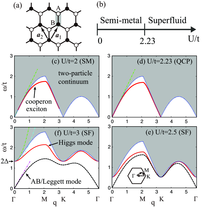
Figure 1: Isotropic honeycomb lattice with basis vectors (a). Phase diagram of the attractive Hubbard model on a honeycomb lattice at half-filling with $t^{\prime}=0$ as obtained from the mean-field theory (b). Evolution of the elementary excitations across the quantum critical point (QCP) of the semi-metal (SM) to superfluid (SF) phase transition (c)-(f). The dash-dot line in each panel and the dash-dot-dot lines in (f) show the asymptotic dispersions of the continuum edge and the superfluid collective modes for small $q$, respectively.

Fig. 1(b) shows the phase diagram of this model at half-filling. Our key findings are summarized in Fig. 1(c)-(f): (i) there are sharp collective mode excitations on either side of the transition. The two-particle continuum is shown as the shaded region, note the window structure. (ii) In the semi-metal phase, there are three degenerate collective modes with “Cooperon” and exciton character. (iii) On the superfluid side, there is a Goldstone mode and remarkably, a distinct superfluid amplitude (Higgs) mode. These modes can be observed in a cold atoms experiment using Bragg scattering. This is a rare example wherein relevant collective excitations can be tracked across a quantum phase transition.

Mean field theory– The ETH group Tarruell has studied fermions loaded onto a honeycomb optical lattice with tunable anisotropy. We consider the attractive Hubbard model in the isotropic honeycomb lattice. As discussed in Ref. Tsuchiya , the isotropic limit is expected to have the highest superfluid transition temperature and is the most promising for experimental realization. We decompose the Hubbard interaction in the superfluid channel using the order parameter $\Delta=U\langle c_{i\downarrow}c_{i\uparrow}\rangle$, taken to be real. For brevity, we introduce a vector operator consisting of creation and annihilation operators $\hat{\Psi}(\bm{p})=(c_{\bm{p},a,\uparrow},c^{\dagger}_{-\bm{p},a,\downarrow},c_{\bm{p},b,\uparrow},c^{\dagger}_{-\bm{p},b,\downarrow})^{t}$ ($a$ and $b$ denote the two sublattices as shown in Fig. 1(a)). The mean field Hamiltonian can be written as $H_{\rm MF}=\sum_{\bm{p}}\hat{\Psi}^{\dagger}(\bm{p})\hat{h}(\bm{p})\hat{\Psi}(\bm{p})$, where $\hat{h}(\bm{p})=\{x_{\bm{p}}+{\rm Re}(\gamma_{\bm{p}})\sigma_{x}-{\rm Im}(\gamma_{\bm{p}})\sigma_{y}\}\tau_{3}-\Delta\tau_{1}$, $\gamma_{\bm{p}}=-t(1+e^{i\bm{p}\cdot\bm{a}_{1}}+e^{i\bm{p}\cdot\bm{a}_{2}})$ and $x_{\bm{p}}=-2t^{\prime}[\cos(\bm{p}\cdot\bm{a}_{1})+\cos(\bm{p}\cdot\bm{a}_{2})+\cos(\bm{p}\cdot(\bm{a}_{1}-\bm{a}_{2}))]-\mu$ with $\bm{a}_{1}$ and $\bm{a}_{2}$ being the two basis vectors shown in Fig. 1 (a). We take the lattice spacing to be unity. $\vec{\tau}$ and $\vec{\sigma}$ are the Pauli matrices in the Nambu and sublattice space, respectively. The single-particle Green’s function for the mean-field Hamiltonian is given by

$$\hat{G}(p)=\left[i\omega_{n}-\hat{h}(\bm{p})\right]^{-1}\equiv\left(\begin{array}[]{cc}\hat{G}^{aa}(p)&\hat{G}^{ab}(p)\\ \hat{G}^{ba}(p)&\hat{G}^{bb}(p)\end{array}\right).$$ (4)

Here, we denote $p=(\bm{p},i\omega_{n})$, where $\omega_{n}$ is the fermion Matsubara frequency. The gap and number equations are obtained from the off-diagonal and diagonal elements of the Green’s function ${\hat{G}}^{\nu\nu}$ as Zhao (hereafter, we restrict ourselves to zero temperature)

$$\frac{1}{U} = \frac{1}{N}\sum_{\bm{p}}\sum_{\alpha=\pm}\frac{1}{2E^{\alpha}(\bm{p})},$$ (5)

$$n = 1-\frac{1}{N}\sum_{\bm{p}}\sum_{\alpha=\pm}\frac{\xi_{\bm{p}}^{\alpha}}{E^{\alpha}(\bm{p})},$$ (6)

where $E^{\pm}(\bm{p})=\sqrt{(\xi_{\bm{p}}^{\pm})^{2}+\Delta^{2}}$ is the spectrum of the Bogoliubov quasiparticles, $\xi_{\bm{p}}^{\pm}=x_{\bm{p}}\pm|\gamma_{\bm{p}}|$, and $N$ is the number of lattice sites. At half-filling, the self-consistent solution of $\Delta$ becomes non-zero for $U>U_{c}$ indicating a transition from semi-metal to superfluid phases Zhao ; Tsuchiya . For $t^{\prime}=0$, mean-field theory gives $U_{c}\sim 2.23t$. Quantum Monte Carlo gives the same transition, except with $U_{c}$ renormalized to $\sim 3.869$ Sorella . In the rest of this letter, we use mean-field results with the understanding that fluctuations will renormalize $U$ quantitatively. We note that $U_{c}$ weakly depends on the value of $t^{\prime}$.

Generalized Random Phase Approximation (GRPA)– On either side of the critical point, there are low-lying density and pairing fluctuations. We use a generalized random phase approximation (GRPA) scheme to evaluate density and pairing response functions. We follow the Green’s function approach of Côté and Griffin Cote . We denote matrix susceptibilities containing the response to weak density and pairing perturbations, respectively, as

$$\hat{L}^{\nu_{1}\nu_{2}}(q)=\left(\begin{array}[]{cc}\chi^{\nu_{1}\nu_{2}}_{n_{\uparrow}n}(q)&\chi^{\nu_{1}\nu_{2}}_{mn}(q)\\ -\chi^{\nu_{1}\nu_{2}}_{m^{\dagger}n}(q)&\chi^{\nu_{1}\nu_{2}}_{n_{\downarrow}n}(q)\end{array}\right),$$ (9)

$$\hat{M}^{\nu_{1}\nu_{2}}(q)=\left(\begin{array}[]{cc}\chi^{\nu_{1}\nu_{2}}_{n_{\uparrow}m^{\dagger}}(q)&\chi^{\nu_{1}\nu_{2}}_{mm^{\dagger}}(q)\\ -\chi^{\nu_{1}\nu_{2}}_{m^{\dagger}m^{\dagger}}(q)&\chi^{\nu_{1}\nu_{2}}_{n_{\downarrow}m^{\dagger}}(q)\end{array}\right),$$ (12)

where $q=(\bm{q},i\Omega_{n})$ ($\Omega_{n}$ is a boson Matsubara frequency). Any susceptibility $\chi$ is defined as

$$\chi_{fg}^{\nu_{1}\nu_{2}}(q)=-\sum_{\bm{r}_{12}}\int_{0}^{\beta}d\tau_{12}\langle T_{\tau}\delta f(1)\delta g(2)\rangle e^{-i(\bm{q}\cdot\bm{r}_{12}-\Omega_{n}\tau_{12})},$$ (13)

where $1\equiv(\bm{r}_{l_{1}},\nu_{1},\tau_{1})$ ($l_{1}$ denotes the unit cell, $\nu_{1}$ the sublattice, and $\tau_{1}$ an imaginary time), $\bm{r}_{12}=\bm{r}_{l_{1}}-\bm{r}_{l_{2}}$, $\tau_{12}=\tau_{1}-\tau_{2}$ and $\delta f\equiv f-\langle f\rangle$. The density and pair annihilation operators are written as $n=n_{\uparrow}+n_{\downarrow}$ and $m=c_{\downarrow}c_{\uparrow}$, respectively. The GRPA equations read Tsuchiya ; Cote

$${\bar{A}}^{\nu_{1}\nu_{2}}(q) = \hat{A}^{0\nu_{1}\nu_{2}}(q)+\frac{2U}{\beta N}\sum_{\nu_{3}}\sum_{\bm{p},\omega_{n}}{\tilde{G}}^{\nu_{1}\nu_{3}}(p+q)$$ (14)

$$\times{\bar{A}}^{\nu_{3}\nu_{2}}(q){\tilde{G}}^{\nu_{3}\nu_{1}}(p),$$

$$\hat{A}^{\nu_{1}\nu_{2}}(q)\! = \!\!\!{\bar{A}}^{\nu_{1}\nu_{2}}(q)\!-\!U\!\sum_{\nu_{3}}{\bar{L}}^{\nu_{1}\nu_{3}}(q)\mathrm{Tr}\{\hat{A}^{\nu_{3}\nu_{2}}(q)\},$$ (15)

where $A$ is either $L$ or $M$ and ${\tilde{G}}^{\nu_{1}\nu_{2}}(p)=\tau_{3}\hat{G}^{\nu_{1}\nu_{2}}(p)$. $A^{0}$ denotes the bare susceptibility bareA0 , $\bar{A}$ includes an infinite sum over ladder diagrams, while $\hat{A}$ is the final result which also includes bubble diagrams.

Undamped Higgs mode– In the superfluid phase, we solve GRPA equations (14) and (15) to evaluate the amplitude and phase correlation functions $\chi_{\Delta\Delta}^{\nu_{1}\nu_{2}}(q)=\frac{U^{2}}{2}(\chi_{mm^{\dagger}}^{\nu_{1}\nu_{2}}(q)+\chi_{m^{\dagger}m^{\dagger}}^{\nu_{1}\nu_{2}}(q))$ and $\chi_{\theta\theta}^{\nu_{1}\nu_{2}}(q)=\frac{U^{2}}{2\Delta^{2}}(\chi_{mm^{\dagger}}^{\nu_{1}\nu_{2}}(q)-\chi_{m^{\dagger}m^{\dagger}}^{\nu_{1}\nu_{2}}(q))$. The amplitude and phase fluctuation operators are given by $\delta\Delta=\frac{U}{2}(\delta m+\delta m^{\dagger})$ and $\delta\theta=\frac{U}{2i\Delta}(\delta m-\delta m^{\dagger})$, respectively. For the case of $t^{\prime}=0$, the expressions simplify and we can identify their respective poles, which we denote “Higgs” and “AB/Leggett”. These poles satisfy

$$Higgs:\phantom{a}\frac{1}{U} = -(C+D)+|R|,$$ (16)

$$AB/Leggett:\phantom{a}\frac{1}{U} = -(C-D)+\sqrt{4F^{2}+|R|^{2}}.\ \$$ (17)

We have defined

$$C = \frac{1}{N}\sum_{\bm{p}}\frac{E+E^{\prime}}{(i\Omega_{n})^{2}-(E+E^{\prime})^{2}},$$ (18)

$$D = -\frac{1}{N}\sum_{\bm{p}}\frac{\Delta^{2}}{E^{\prime}E}\frac{E+E^{\prime}}{(i\Omega_{n})^{2}-(E+E^{\prime})^{2}},$$ (19)

$$F = \frac{1}{N}\sum_{\bm{p}}\frac{\Delta}{E}\frac{i\Omega_{n}}{(i\Omega_{n})^{2}-(E+E^{\prime})^{2}},$$ (20)

$$R = -\frac{1}{N}\sum_{\bm{p}}\frac{\gamma^{\prime}\gamma^{*}}{E^{\prime}E}\frac{E+E^{\prime}}{(i\Omega_{n})^{2}-(E+E^{\prime})^{2}}.$$ (21)

Here, we have denoted $E=E(\bm{p})$, $E^{\prime}=E(\bm{p}+\bm{q})$, $\gamma=\gamma_{\bm{p}}$, and $\gamma^{\prime}=\gamma_{\bm{p}+\bm{q}}$. On the other hand, solving Eqs. (14) and (15) for density response, we find that $\chi_{\theta\theta}^{\nu_{1}\nu_{2}}(q)\propto\chi_{nn}^{\nu_{1}\nu_{2}}(q)$ when $t^{\prime}=0$. Thus, the density response function only retains the AB/Leggett pole given in Eq. (17).

Setting $\bm{q}=\Omega_{n}=0$ in Eq. (17), we recover the gap equation (5). Thus, the superfluid phase has gapless collective mode(s) arising from phase fluctuations. In fact, at half-filling, the AB/Leggett pole in Eq. (17) is a double pole corresponding to two gapless modes: the Anderson-Bogoliubov (AB) mode and the Leggett mode Tsuchiya . The AB mode is the usual Goldstone mode associated with U(1) symmetry breaking Anderson ; Nambu . The Leggett mode is composed of out-of-phase fluctuations between sublattices Leggett - it acquires a gap away from half-filling Tsuchiya . The AB and Leggett modes become degenerate at half-filling reflecting a special pseudospin SU(2) symmetry of the Hubbard model Tsuchiya . For small $q\ll 1$, Eq. (17) gives the dispersion relation of the AB/Leggett mode to be Supple

$$\omega_{\rm AB}=\lambda v_{F}q,\ \ \lambda^{2}=\frac{U}{N}\sum_{\bm{p}}\frac{|\gamma|^{2}}{E^{3}}\leq 1,$$ (22)

where $v_{F}=3t/2$ is the Fermi velocity at the Dirac points.

Setting $(\bm{q},i\Omega_{n})=(0,2\Delta)$, Eq. (16) also reduces to the gap equation. Thus, there exists a gapped collective mode with the energy gap $2\Delta$ at $\bm{q}=0$. This is the ‘Higgs’ mode or the amplitude mode Littlewood arising from amplitude fluctuations of the superfluid order parameter. It can be understood using the mechanical analog of motion along the radial direction of the famous “Mexican hat” potential; the energy gap stems from the finite curvature of the potential along the radial direction.

Remarkably, the Higgs mode disperses below the quasiparticle pair continuum in Figs. 1(e) and (f). In particular, close to the $M$ point, it is well separated from the lower edge of the continuum. This is to be contrasted with the case of typical superfluids: due to the underlying Fermi surface, the continuum exhibits a horizontal edge near $q\sim 0$ Littlewood . The Higgs mode therefore enters the continuum, becomes heavily damped and is unobservable.

In our case, the Higgs mode in Fig. 1 is undamped over large sections of the Brillouin zone. For $q\ll 1$, solving Eq. (16), the Higgs mode has the dispersion relation $\omega_{\rm Higgs}^{2}=4\Delta^{2}+v_{F}^{2}q^{2}$ Supple . The Higgs mode disperses below the lower edge of the continuum which is given by $\omega_{\rm edge}^{2}={\rm min}_{\bm{p}}[(E(\bm{p})+E(\bm{p}+\bm{q}))^{2}]\simeq 4\Delta^{2}+2v_{F}^{2}q^{2}$ ($q\ll 1$). This window or arch in the continuum, shown in Fig. 1, is a consequence of the Dirac-like dispersion of underlying fermions. The Higgs mode stays undamped as long as it lies within this window. Even if we go slightly away from half-filling, the Higgs mode survives undamped. Close to $n\sim 0.9$ or $n\sim 1.1$, the window disappears because of the presence of the Fermi surface - as a result, the Higgs mode is strongly damped. The Higgs mode, the AB mode, and the lower edge of the continuum become degenerate at the QCP for $q\ll 1$: $\omega_{\rm AB}=\omega_{\rm Higgs}=\omega_{\rm edge}=v_{F}q$.

The AB mode and Leggett mode are strongly coupled with density fluctuations; they appear as poles in the density response function $\chi_{nn}^{\nu_{1}\nu_{2}}(q)$. However, when $t^{\prime}=0$, the Higgs mode has no corresponding pole in the density response function. Thus, the Higgs mode is composed of pure amplitude fluctuations and cannot be excited by a density perturbation. This reflects the underlying SU(2) pseudospin symmetry Tsuchiya in the problem. A small finite $t^{\prime}$ breaks this symmetry and forces the Higgs mode to acquire a density component: the density response then shows a peak at the Higgs mode, as shown in Fig.2.

Collective modes in the semi-metal phase: Cooperons and excitons– In the semi-metal phase, setting $\Delta=0$, density and pair response functions become decoupled in the GRPA equations (14)-(15). The susceptibilities satisfy the usual RPA equations $\chi_{mm^{\dagger}}^{\nu_{1}\nu_{2}}(q)=\chi_{mm^{\dagger}}^{0\nu_{1}\nu_{2}}(q)+U\sum_{\nu_{3}}\chi_{mm^{\dagger}}^{0\nu_{1}\nu_{3}}(q)\chi_{mm^{\dagger}}^{\nu_{3}\nu_{2}}(q)$, $\chi_{n_{\sigma}n}^{\nu_{1}\nu_{2}}(q)=\chi_{n_{\sigma}n}^{0\nu_{1}\nu_{2}}(q)-U\sum_{\nu_{3}}\chi_{n_{\sigma}n}^{0\nu_{1}\nu_{3}}(q)\chi_{n_{-\sigma}n}^{\nu_{3}\nu_{2}}(q)$. The bare susceptibility $\chi_{mm^{\dagger}}^{0}$ describes a single rung diagram with particle-particle (hole-hole) excitations, and $\chi_{n_{\sigma}n}^{0}$ describes a single bubble diagram with particle-hole excitations. They are given by

$$\chi_{mm^{\dagger}}^{0\nu_{1}\nu_{2}}(q)=\frac{1}{2N}\sum_{\bm{p}}\left[\frac{\kappa^{\nu_{1}\nu_{2}}_{\bm{p}}\kappa^{\nu_{1}\nu_{2}}_{\bm{q}-\bm{p}}}{\xi_{\bm{p}}^{+}+\xi_{\bm{q}-\bm{p}}^{+}-i\Omega_{n}}-\frac{\eta^{\nu_{1}\nu_{2}}_{\bm{p}}\eta^{\nu_{1}\nu_{2}}_{\bm{q}-\bm{p}}}{\xi_{\bm{p}}^{-}+\xi_{\bm{q}-\bm{p}}^{-}-i\Omega_{n}}\right],\ \ \$$ (23)

$$\chi_{n_{\sigma}n}^{0\nu_{1}\nu_{2}}(q)=\frac{1}{2N}\sum_{\bm{p}}\left[\frac{-\kappa^{\nu_{1}\nu_{2}}_{\bm{p}+\bm{q}}\eta^{\nu_{2}\nu_{1}}_{\bm{p}}}{\xi_{\bm{p}+\bm{q}}^{+}-\xi_{\bm{p}}^{-}-i\Omega_{n}}+\frac{\eta_{\bm{p}+\bm{q}}^{\nu_{1}\nu_{2}}\kappa_{\bm{p}}^{\nu_{2}\nu_{1}}}{\xi_{\bm{p}+\bm{q}}^{-}-\xi_{\bm{p}}^{+}-i\Omega_{n}}\right],\ \ \$$ (24)

where $\kappa_{\bm{p}}^{\nu_{1}\nu_{2}}=\delta_{\nu_{1}\nu_{2}}+e^{i\phi_{\bm{p}}}\delta_{\nu_{1}a}\delta_{\nu_{2}b}+e^{-i\phi_{\bm{p}}}\delta_{\nu_{1}b}\delta_{\nu_{2}a}$ and $\eta_{\bm{p}}^{\nu_{1}\nu_{2}}=\delta_{\nu_{1}\nu_{2}}-e^{i\phi_{\bm{p}}}\delta_{\nu_{1}a}\delta_{\nu_{2}b}-e^{-i\phi_{\bm{p}}}\delta_{\nu_{1}b}\delta_{\nu_{2}a}$. We denote $e^{i\phi_{\bm{p}}}=\gamma_{\bm{p}}/|\gamma_{\bm{p}}|$.

From the denominator in Eq. (23), we see that pairing response arises from particle–particle (or hole–hole) excitations. An undamped pairing mode, occurring below the particle–particle continuum in Fig. 1(c), is therefore a two particle bound state with well defined momentum and energy. It can be understood as a preformed Cooper pair – we call this a Cooperon excitation Rice . Similarly, from Eq. (24), we see that density response arises from particle–hole excitations. An undamped density mode is thus a particle-hole bound state – we call this an exciton.

The dispersions of Cooperons and excitons are determined by the poles of the corresponding response functions, giving $|\hat{I}-U\hat{\chi}_{mm^{\dagger}}(q)|=0$ and $|\hat{I}+U\hat{\chi}_{n_{\sigma}n}^{0}(q)|=0$. With $t^{\prime}=0$, these reduce to the identical equation

$$(1+U\alpha(q))^{2}-U^{2}|\beta(q)|^{2}=0,$$ (25)

$$\alpha(q)=\frac{1}{N}\sum_{\bm{p}}\frac{|\gamma_{\bm{p}}|+|\gamma_{\bm{p}+\bm{q}}|}{(i\Omega_{n})^{2}-(|\gamma_{\bm{p}}|+|\gamma_{\bm{p}+\bm{q}}|)},$$ (26)

$$\beta(q)=-\frac{1}{N}\sum_{\bm{p}}\frac{e^{i(\phi_{\bm{p}+\bm{q}}-\phi_{\bm{p}})}(|\gamma_{\bm{p}}|+|\gamma_{\bm{p}+\bm{q}}|)}{(i\Omega_{n})^{2}-(|\gamma_{\bm{p}}|+|\gamma_{\bm{p}+\bm{q}}|)^{2}}.$$ (27)

Thus, the Cooperon and the exciton are degenerate when $t^{\prime}=0$. Their dispersion is shown in Figs. 1 (c) and (d) – the modes are undamped as they lie below the two particle continuum. In particular, they are well separated from the continuum in the vicinity of the $M$ points. We suggest that experiments should probe this region to observe the collective excitations. This feature of the $M$ points can be understood from the single particle band structure which has saddle points at these wavevectors. They consequently have a very large density of states which provides large phase space for the Hubbard interaction to form two–particle bound states.

These collective modes in the semi-metal phase were predicted many years ago – using an insightful single-cone approximation – Ref. Baskaran reported a triplet exciton mode in the repulsive Hubbard model. The authors identified the window structure in the continuum as capable of accommodating stable modes. Mapping their results to the attractive Hubbard case p-hmapping , the triplet excitons translate to Cooperon and exciton modes. We reaffirm their prediction starting from a microscopic picture taking into account the sublattice structure. Our expressions also agree with those of Ref. Peres – which only considers the $\Gamma-K$ segment and concludes that there is no undamped mode. However, we find an undamped mode in the $\Gamma-M$ and $M-K$ directions.

Cooperon condensation– As we approach the critical point from the semi-metal side, the energy of the Cooperon and exciton decreases progressively (see Fig. 1(c) and (d)). Precisely at the transition, the Cooperon “softens” at $\bm{q}=0$ and undergoes condensation. In fact, setting $\bm{q}=\Omega_{n}=0$, the Cooperon pole in Eq. (25) reduces to the gap equation (5). Since Cooperons and excitons are degenerate for $t^{\prime}=0$, the exciton can also condense at the critical point. That gives rise to the sublattice–CDW state - which is degenerate with the superfluid state due to SU(2) pseudospin symmetry. For $t^{\prime}\neq 0$, this degeneracy is lifted in favour of the superfluid and the Cooperon condenses preferentially.

As we cross $U_{c}$ and enter the superfluid phase, Cooperons and excitons hybridize to become the AB, Leggett and Higgs modes. The excitonic component, when present, allows these modes to have peaks in the density response function. The Cooperonic component manifests as peaks in the pairing response. Thus, the collective modes evolve smoothly across the QCP and carry signatures of the underlying spontaneous symmetry breaking.

Visibility of the Higgs mode–

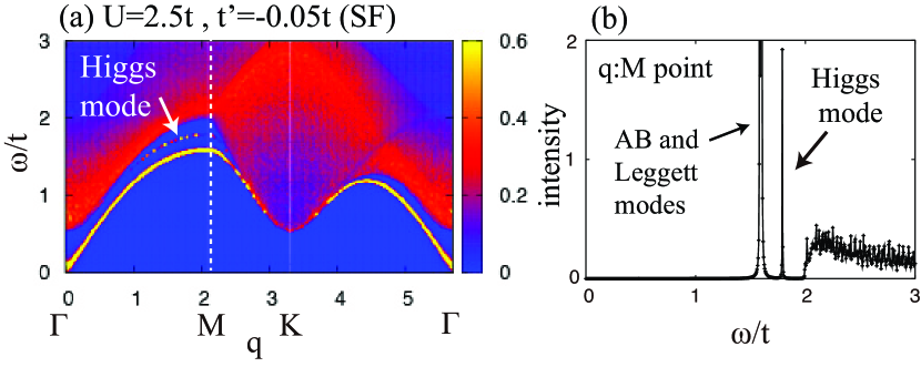
Figure 2: Intensity of dynamic structure factor corresponding to density response $S(\bm{q},\omega)=-{\rm Im}[\chi_{nn}(\bm{q},\omega)]/\pi$ for $t^{\prime}=-0.05t$ (a). The cross section for the momentum at the $M$ point (b). The upper peak corresponds to the Higgs mode.

Our Higgs mode is stable against decay into pairs of fermions due to the window structure in the two particle continuum. However, if we go beyond RPA level, the Higgs mode may decay by emitting AB/Leggett excitations which are lower in energy. We argue that this merely leads to broadening of the Higgs mode. In our semi-metal to superfluid transition, due to the pseudospin symmetry present when $t^{\prime}=0$, the order parameter can be thought of as an O(3) object. Quantum Monte Carlo simulations of the O(3) ordering transition show that the Higgs mode survives although it is broadened by decay into Goldstone bosons Gazit . We expect this to be true in our case as well.

We suggest Bragg spectroscopy measurements on a Fermi superfluid in a honeycomb optical lattice as a way to measure this undamped Higgs mode. In this technique, a two-photon process imparts a density-“kick” to the system. The response to this perturbation can be quantified by measuring the momentum transferred or the energy absorbed. The momentum transferred is a measure of the dynamic structure factor related to the density response function $S(\bm{q},\omega)=-{\rm Im}[\chi_{nn}(\bm{q},\omega)]/\pi$ Pitaevskii – it can detect collective modes as long as they have a density component. For any small $t^{\prime}\neq 0$, the Higgs mode in our model has a density component which makes it visible to Bragg spectroscopy. A small $t^{\prime}$ hopping is expected to be present in an optical lattice setup any way Ibanez . Figure 2 shows $S(\bm{q},\omega)$ for $t^{\prime}=-0.05$. The sharp intensity peak for the Higgs mode can be clearly seen below the continuum. An alternative approach is to measure the energy absorption in response to a weak shaking of the optical lattice Endres .

Acknowledgements–We acknowledge A. Paramekanti for fruitful dicussions. S.T. thanks M. Sigrist, T. Esslinger, L. Tarruell, Y. Ohashi, S. Okada, S. Konabe, K. Asano, S. Kurihara, and K. Kamide for discussions. S. T. was supported by Grant-in-Aid for Scientific Research, No. 24740276.

I Supplementary Materials

I.1 Bare susceptibility in GRPA

To solve the GRPA equations (8) and (9), the bare susceptibilities $L^{0}$ and $M^{0}$ are evaluated using the mean-field Green’s function in Eq. (2) to give

$$\hat{L}^{0\nu_{1}\nu_{2}}(q)=\frac{1}{\beta M}\sum_{\bm{p},\omega_{n}}{\tilde{G}}^{\nu_{1}\nu_{2}}(p+q){\tilde{G}}^{\nu_{2}\nu_{1}}(p)$$

$$=\left(\begin{array}[]{cc}L^{0\nu_{1}\nu_{2}}_{1111}+L^{0\nu_{1}\nu_{2}}_{1221}&L^{0\nu_{1}\nu_{2}}_{1112}+L^{0\nu_{1}\nu_{2}}_{1222}\\ L^{0\nu_{1}\nu_{2}}_{2111}+L^{0\nu_{1}\nu_{2}}_{2221}&L^{0\nu_{1}\nu_{2}}_{2112}+L^{0\nu_{1}\nu_{2}}_{2222}\end{array}\right),$$ (30)

$$\hat{M}^{0\nu_{1}\nu_{2}}(q)=\frac{1}{\beta M}\sum_{\bm{p},\omega_{n}}{\tilde{G}}^{\nu_{1}\nu_{2}}(p+q)\left(\begin{array}[]{cc}0&1\\ 0&0\end{array}\right){\tilde{G}}^{\nu_{2}\nu_{1}}(p)$$ (33)

$$=\left(\begin{array}[]{cc}L^{0\nu_{1}\nu_{2}}_{1121}&L^{0\nu_{1}\nu_{2}}_{1122}\\ L^{0\nu_{1}\nu_{2}}_{2121}&L^{0\nu_{1}\nu_{2}}_{2122}\end{array}\right),$$ (36)

where we introduced the tensor

$$L^{0\nu_{1}\nu_{2}}_{ijkl}(q)=\frac{2}{\beta N}\sum_{\bm{p},\omega_{n}}{\tilde{G}}_{ij}^{\nu_{1}\nu_{2}}(p+q){\tilde{G}}_{kl}^{\nu_{2}\nu_{1}}(p).$$ (37)

Following Ref. Cote , we introduce a column vector $\mathcal{A}$($={\mathcal{L}},{\mathcal{M}}$) and a $4\times 4$ matrix $\mathcal{D}$ as

$$\mathcal{A}=\left(\begin{array}[]{c}A_{11}\\ A_{12}\\ A_{21}\\ A_{22}\end{array}\right)\equiv\left(\begin{array}[]{c}A_{1}\\ A_{2}\\ A_{3}\\ A_{4}\end{array}\right),$$ (46)

$$\hat{\mathcal{D}}=\left(\begin{array}[]{cccc}L^{0}_{1111}&L^{0}_{1121}&L^{0}_{1211}&L^{0}_{1221}\\ L^{0}_{1112}&L^{0}_{1122}&L^{0}_{1212}&L^{0}_{1222}\\ L^{0}_{2111}&L^{0}_{2121}&L^{0}_{2211}&L^{0}_{2221}\\ L^{0}_{2112}&L^{0}_{2122}&L^{0}_{2212}&L^{0}_{2222}\end{array}\right).$$ (51)

The GRPA equations are cast into the form

$$\bar{\mathcal{A}}^{\nu_{1}\nu_{2}}(q)={\mathcal{A}}^{0\nu_{1}\nu_{2}}(q)+U\sum_{\nu_{3}}\hat{\mathcal{D}}^{\nu_{1}\nu_{3}}(q)\bar{\mathcal{A}}^{\nu_{3}\nu_{2}}(q),$$ (52)

$$\mathcal{A}^{\nu_{1}\nu_{2}}(q)=\bar{\mathcal{A}}^{\nu_{1}\nu_{2}}(q)-U\sum_{\nu_{3}}\bar{\mathcal{L}}^{\nu_{1}\nu_{3}}(q)A^{\nu_{3}\nu_{2}}(q).$$ (53)

The above equations are easily solved to give

$$\left(\begin{array}[]{cc}A^{aa}(q)&A^{ab}(q)\\ A^{ba}(q)&A^{bb}(q)\end{array}\right)=\left(\begin{array}[]{cc}1+U{\bar{L}}^{aa}(q)&U{\bar{L}}^{ab}(q)\\ U{\bar{L}}^{ba}(q)&1+U{\bar{L}}^{bb}(q)\end{array}\right)^{-1}\left(\begin{array}[]{cc}\bar{A}^{aa}(q)&\bar{A}^{ab}(q)\\ \bar{A}^{ba}(q)&\bar{A}^{bb}(q)\end{array}\right),$$ (60)

$$\left(\begin{array}[]{cc}\bar{\mathcal{A}}^{aa}(q)&\bar{\mathcal{A}}^{ab}(q)\\ \bar{\mathcal{A}}^{ba}(q)&\bar{\mathcal{A}}^{bb}(q)\end{array}\right)=\left(\begin{array}[]{cc}\hat{I}-U\hat{\mathcal{D}}^{aa}(q)&-U\hat{\mathcal{D}}^{ab}(q)\\ -U\hat{\mathcal{D}}^{ba}(q)&\hat{I}-U\hat{\mathcal{D}}^{bb}(q)\end{array}\right)^{-1}\left(\begin{array}[]{cc}{\mathcal{A}}^{0aa}(q)&{\mathcal{A}}^{0ab}(q)\\ {\mathcal{A}}^{0ba}(q)&{\mathcal{A}}^{0bb}(q)\end{array}\right).$$ (67)

Here, we denoted $A^{\nu_{1}\nu_{2}}={\rm Tr}\{\hat{A}^{\nu_{1}\nu_{2}}\}={\mathcal{A}}_{1}^{\nu_{1}\nu_{2}}+{\mathcal{A}}_{4}^{\nu_{1}\nu_{2}}$.

I.2 Energy dispersion of the Higgs mode

We derive the analytic expression of the energy dispersion of the Higgs mode for small momentum $q\ll 1$ following the approach of Ref. Littlewood . The gap equation (5) can be rewritten as

$$1-\frac{U}{2N}\sum_{\bm{p}}\left(\frac{1}{E}+\frac{1}{E^{\prime}}\right)=0.$$ (68)

We denote $E(\bm{p})=E$, $E(\bm{p}+\bm{q})=E^{\prime}$, $\gamma=\gamma_{\bm{p}}$, and $\gamma^{\prime}=\gamma_{\bm{p}+\bm{q}}$. Subtracting Eq. (68) from $1+U[(C+D)-|R|]=0$ which is equivalent to Eq. (16), we obtain

$$U\left(X-|R|\right)=0,$$ (69)

where

$$X=(C+D)+\frac{1}{2N}\sum_{\bm{p}}\frac{E+E^{\prime}}{EE^{\prime}}$$

$$=\frac{1}{2N}\sum_{\bm{p}}\frac{E+E^{\prime}}{EE^{\prime}}\frac{\omega^{2}-(|\gamma|^{2}+|\gamma^{\prime}|^{2})-4\Delta^{2}}{\omega^{2}-(E+E^{\prime})^{2}}.$$ (70)

Here, we have replaced $i\Omega_{n}\to\omega$. At $\bm{q}=0$, Eq. (69) reduces to

$$\frac{y}{N}\sum_{\bm{p}}\frac{1}{E}\frac{1}{\omega^{2}-4E^{2}}$$

$$=y\int_{0}^{3t}d\varepsilon\ \frac{\rho(\varepsilon)}{\sqrt{\varepsilon^{2}+\Delta^{2}}[\omega^{2}-4(\varepsilon^{2}+\Delta^{2})]}=0,$$ (71)

where $y=\omega^{2}/4-\Delta^{2}$ and $\rho(\varepsilon)=\frac{1}{N}\sum_{\bm{p}}\delta(\varepsilon-|\gamma_{\bm{p}}|)$ is the density of states of the fermion energy band. If we set $\omega=2\Delta$, the denominator in the integrand of Eq. (71) is proportional to $\varepsilon^{2}$, while the numerator is proportional to $\varepsilon$ for small $\varepsilon$ because $\rho(\varepsilon)\propto\varepsilon$. The integral in Eq. (71) is thus well defined in the limit $\omega\to 2\Delta$. In this limit, Eq. (71) is satisfied when $y=0$ and consequently the energy of the Higgs mode is obtained as $\omega_{\rm Higgs}(\bm{q}=0)=2\Delta$.

To derive the energy dispersion for small $\bm{q}$, we expand Eq. (69) to second order in ${\bm{q}}$. Using the relations

$$\gamma_{\bm{p}+\bm{q}}\simeq\gamma_{\bm{p}}+\delta\gamma_{1}+\delta\gamma_{2},\ \delta\gamma_{1}=-it\{e^{i\bm{p}\cdot\bm{a}_{1}}(\bm{q}\cdot\bm{a}_{1})+e^{i\bm{p}\cdot\bm{a}_{2}}(\bm{q}\cdot\bm{a}_{2})\},$$ (72)

$$\delta\gamma_{2}=\frac{t}{2}\{e^{i\bm{p}\cdot\bm{a}_{1}}(\bm{q}\cdot\bm{a}_{1})^{2}+e^{i\bm{p}\cdot\bm{a}_{2}}(\bm{q}\cdot\bm{a}_{2})^{2}\},$$ (73)

$$w_{1}={\rm Re}[\gamma^{*}\delta\gamma_{1}]=-t^{2}\left\{(\sin(\bm{p}\cdot\bm{a}_{1})+\sin(\bm{p}\cdot\bm{a}_{3}))(\bm{q}\cdot\bm{a}_{1})+(\sin(\bm{p}\cdot\bm{a}_{2})-\sin(\bm{p}\cdot\bm{a}_{3}))(\bm{q}\cdot\bm{a}_{2})\right\},$$ (74)

$$w_{1}^{\prime}={\rm Im}[\gamma^{*}\delta\gamma_{1}]=t^{2}\left\{(1+\cos(\bm{p}\cdot\bm{a}_{1})+\cos(\bm{p}\cdot\bm{a}_{3}))(\bm{q}\cdot\bm{a}_{1})+(1+\cos(\bm{p}\cdot\bm{a}_{2})+\cos(\bm{p}\cdot\bm{a}_{3}))(\bm{q}\cdot\bm{a}_{2})\right\},$$ (75)

$$w_{2}={\rm Re}[\gamma^{*}\delta\gamma_{2}]=-\frac{t^{2}}{2}\left\{(1+\cos(\bm{p}\cdot\bm{a}_{1})+\cos(\bm{p}\cdot\bm{a}_{3}))(\bm{q}\cdot\bm{a}_{1})^{2}+(1+\cos(\bm{p}\cdot\bm{a}_{2})+\cos(\bm{p}\cdot\bm{a}_{3}))(\bm{q}\cdot\bm{a}_{2})^{2}\right\},$$ (76)

$$w_{2}^{\prime}={\rm Im}[\gamma^{*}\delta\gamma_{2}]=-\frac{t^{2}}{2}\left\{(\sin(\bm{p}\cdot\bm{a}_{1})+\sin(\bm{p}\cdot\bm{a}_{3}))(\bm{q}\cdot\bm{a}_{1})^{2}+(\sin(\bm{p}\cdot\bm{a}_{2})-\sin(\bm{p}\cdot\bm{a}_{3}))(\bm{q}\cdot\bm{a}_{2})^{2}\right\},$$ (77)

$$|\gamma_{\bm{p}+\bm{q}}|^{2}\simeq|\gamma_{\bm{p}}|^{2}+s_{1}+s_{2},\ \ s_{1}=2w_{1},\ s_{2}=|\delta\gamma_{1}|^{2}+2w_{2},$$ (78)

$$|\delta\gamma_{1}|^{2}=t^{2}\left\{(\bm{q}\cdot\bm{a}_{1})^{2}+2\cos(\bm{p}\cdot\bm{a}_{3})(\bm{q}\cdot\bm{a}_{1})(\bm{q}\cdot\bm{a}_{2})+(\bm{q}\cdot\bm{a}_{2})^{2}\right\},$$ (79)

one finds that Eq. (70) becomes

$$X\simeq\frac{1}{2N}\sum_{\bm{p}}\frac{2}{E}\frac{\omega^{2}-(2|\gamma|^{2}+s_{1}+s_{2})-4\Delta^{2}}{\omega^{2}-4E^{2}}$$

$$=\frac{1}{N}\sum_{\bm{p}}\frac{1}{E}\frac{\omega^{2}-(2|\gamma|^{2}+s_{2})-4\Delta^{2}}{\omega^{2}-4E^{2}}.$$ (80)

Since the factor $\sin(\bm{p}\cdot\bm{a}_{i})$ is odd for $\bm{p}$, the summation for $\bm{p}$ including this factor vanishes. Similarly, $R$ can be approximated as

$$R\simeq-\frac{1}{N}\sum_{\bm{p}}\frac{2}{E}\frac{(\gamma+\delta\gamma_{1}+\delta\gamma_{2})\gamma^{*}}{\omega^{2}-4E^{2}},$$ (81)

$${\rm Re}R=-\frac{1}{N}\sum_{\bm{p}}\frac{2}{E}\frac{|\gamma|^{2}+w_{2}}{\omega^{2}-4E^{2}}=R_{0}+R_{2},$$ (82)

$${\rm Im}R=-\frac{1}{N}\sum_{\bm{p}}\frac{2}{E}\frac{w_{1}^{\prime}}{\omega^{2}-4E^{2}}=R_{1}.$$ (83)

In evaluating further Eqs. (80), (82), and (83), we encounter the factor

$$\sum_{\bm{p}}\frac{1}{E}\frac{\cos(\bm{p}\cdot\bm{a}_{i})}{\omega^{2}-4E^{2}}.$$ (84)

Here, we replace $\cos(\bm{p}\cdot\bm{a}_{i})$ in the integrand with its value at the $K$ ($K^{\prime}$) point, i.e., $\langle\cos(\bm{p}\cdot\bm{a}_{i})\rangle=\cos(\bm{p}_{K}\cdot\bm{a}_{i})=-1/2$. At half-filling, since the Fermi level is at the $K$ ($K^{\prime}$) point, this replacement is justified for small $q$. As a result, $R_{1}$ and $R_{2}$ vanish and we finally obtain

$$X-|R|\simeq\left(4y-v_{F}^{2}q^{2}\right)\frac{1}{N}\sum_{\bm{p}}\frac{1}{E}\frac{1}{\omega^{2}-4E^{2}}=0,$$ (85)

where $v_{F}=3t/2$ is the Fermi velocity. Consequently, the dispersion of the Higgs mode is obtained as

$$\omega_{\rm Higgs}^{2}=4\Delta^{2}+v_{F}^{2}q^{2}.$$ (86)

In the limit $\Delta^{2}\gg v_{F}^{2}q^{2}$, $\omega_{\rm Higgs}$ is approximated as $\omega_{\rm Higgs}=2\Delta+v_{F}^{2}q^{2}/4\Delta$ which is plotted in Fig. 1 (f). On the other hand, at the transition point with $\Delta=0$, the dispersion for small $q$ coincides with that of the lower edge of the continuum as $\omega_{\rm Higgs}=v_{F}q.$

I.3 Energy dispersion of the AB/Leggett mode

We derive the energy dispersion of the AB/Leggett mode for small momentum. Subtracting Eq. (68) from $1+U[(C-D)-\sqrt{4F^{2}+|R|^{2}}]=0$ which is equivalent to Eq. (11), we obtain

$$U\left(Y-\sqrt{4F^{2}+|R|^{2}}\right)=0,$$ (87)

where

$$Y=(C-D)+\frac{1}{2N}\sum_{\bm{p}}\frac{E+E^{\prime}}{EE^{\prime}}$$

$$=\frac{1}{2N}\sum_{\bm{p}}\frac{E+E^{\prime}}{EE^{\prime}}\frac{\omega^{2}-(|\gamma|^{2}+|\gamma^{\prime}|^{2})}{\omega^{2}-(E+E^{\prime})^{2}}.$$ (88)

Setting $\bm{q}=0$, we obtain

$$Y = \frac{1}{N}\sum_{\bm{p}}\frac{1}{E}\frac{\omega^{2}-2|\gamma|^{2}}{\omega^{2}-4E^{2}}=d_{1}\omega^{2}-2d_{2},$$ (89)

$$R = -\frac{2}{N}\sum_{\bm{p}}\frac{1}{E}\frac{|\gamma|^{2}}{\omega^{2}-4E^{2}}=-2d_{2},$$ (90)

$$F = \frac{1}{N}\sum_{\bm{p}}\frac{1}{E}\frac{\Delta\omega}{\omega^{2}-4E^{2}}=d_{2}\Delta\omega,$$ (91)

where

$$d_{1}(\omega)=\frac{1}{N}\sum_{\bm{p}}\frac{1}{E}\frac{1}{\omega^{2}-4E^{2}},$$ (92)

$$\ d_{2}(\omega)=\frac{1}{N}\sum_{\bm{p}}\frac{1}{E}\frac{|\gamma|^{2}}{\omega^{2}-E^{2}}.$$ (93)

Thus, Eq. (87) reduces to

$$Y-\sqrt{4F^{2}+|R|^{2}}$$

$$=\frac{d_{1}\omega^{2}(d_{1}\omega^{2}-4d_{2}-4d_{1}\Delta^{2})}{(d_{1}\omega^{2}-2d_{2})+\sqrt{4d_{1}^{2}\Delta^{2}\omega^{2}+4d_{2}^{2}}}=0.$$ (94)

From $d_{i=1,2}(\omega<2\Delta)<0$, we obtain the gapless AB/Leggett mode: $\omega_{\rm AB}(\bm{q}=0)=0$. Note that the term within parentheses in the numerator of Eq. (94) at $\omega=0$ is found to give

$$-4d_{2}(\omega=0)-4d_{1}(\omega=0)\Delta^{2}=\frac{1}{N}\sum_{\bm{p}}\frac{1}{E}=\frac{1}{U}.$$ (95)

For small $\bm{q}$, expanding $F$, $R$, and $Y$ to second order in $\bm{q}$, we obtain

$$Y\simeq d_{1}\omega^{2}-2d_{2}-d_{1}v_{F}^{2}q^{2},$$ (96)

$$F\simeq\Delta d_{1}\omega,\ \ R\simeq-2d_{2}.$$ (97)

In Eqs. (96) and (97), we used the same approximation as the one for Eq. (85). As a result, we obtain

$$Y-\sqrt{4F^{2}+|R|^{2}}$$

$$\simeq\frac{d_{1}(\omega=0)(\omega^{2}/U+4d_{2}(\omega=0)v_{F}^{2}q^{2})}{(d_{1}\omega^{2}-2d_{2}-2d_{1}v_{F}^{2}q^{2})+\sqrt{4\Delta^{2}d_{1}^{2}\omega^{2}+4d_{2}^{2}}}$$

$$=0.$$ (98)

We have used Eq. (95) to derive the final expression. The pole is thus given by

$$\omega_{\rm AB}=\lambda v_{F}q,$$ (99)

$$\lambda^{2}=4U|d_{2}(\omega=0)|=\frac{U}{N}\sum_{\bm{p}}\frac{|\gamma|^{2}}{E^{3}}.$$ (100)

Note that $\lambda\leq 1$ from the gap equation (2). At the transition point ($\Delta=0$), $\lambda=1$ and thus the AB/Leggett mode becomes degenerate with the Higgs mode as well as the edge of the continuum as $\omega_{\rm AB}=v_{F}q$.

References

• (1) C. M. Varma, J. Low Temp. Phys. 126, 902 (2002).
• (2) R. Sooryakumar and M. V. Klein, Phys. Rev. Lett. 45, 660 (1980).
• (3) P. B. Littlewood and C. M. Varma, Phys. Rev. Lett. 47, 811 (1981); Phys. Rev. B 26, 4883 (1982).
• (4) K. Penc et al., Phys. Rev. Lett. 108, 257203 (2012).
• (5) Ch. Rüegg et al., Phys. Rev. Lett. 100, 205701 (2008).
• (6) U. Bissbort et al., Phys. Rev. Lett. 106, 205303 (2011).
• (7) M. Endres et al., Nature (London), 487, 454 (2012).
• (8) L. Tarruell, D. Greif, T. Uehlinger, G. Jotzu, and T. Esslinger, Nature 483, 302 (2012).
• (9) I. Bloch, J. Dalibard, and W. Zwerger, Rev. Mod. Phys. 80, 885 (2008).
• (10) E. Zhao and A. Paramekanti, Phys. Rev. Lett. 97, 230404 (2006).
• (11) S. Tsuchiya, R. Ganesh, and A. Paramekanti, Phys. Rev. A 86, 033604 (2012).
• (12) S. Sorella, Y. Otsuka, and S. Yunoki, Scientific Rep. 2, 992 (2012).
• (13) Ref. Sorella has used Quantum Monte Carlo simulations to establish the phase diagram of the repulsive Hubbard model with $t^{\prime}=0$. However, this model can be mapped onto the attractive model using a sublattice-dependent particle-hole transformation. See, e.g., S.-C. Zhang, Phys. Rev. Lett. 65, 120 (1990).
• (14) P. Nozieres and F. Pistolesi, Eur. Phys. J. B 10, 649 (1999).
• (15) G. Baskaran and S. A. Jafari, Phys. Rev. Lett. 89, 016402 (2002).
• (16) R. Côté and A. Griffin, Phys. Rev. B 48, 10404 (1993).
• (17) See Supplementary Material for explicit expressions for the bare susceptibility $A^{0}$.
• (18) P. W. Anderson, Phys. Rev. 110, 827 (1958).
• (19) Y. Nambu, Phys. Rev. 117, 648 (1958).
• (20) A. J. Leggett, Prog. Theor. Phys. 36, 901 (1966).
• (21) See Supplementary Material for the detailed derivation of the asymptotic dispersions of the AB/Leggett mode and the Higgs mode.
• (22) T. M. Rice, K.-Y. Yang, and F. C. Zhang, Rep. Prog. Phys. 75, 016502 (2012).
• (23) N. M. R. Peres, M. A. N. Araújo, and A. H. Castro Neto, Phys. Rev. Lett. 92, 199701 (2004).
• (24) S. Gazit, D. Podolsky, and A. Auerbach, arXiv:1212.3759 (2012).
• (25) L. Pitaevskii and S. Stringari, Bose-Einstein Condensation, (Oxford University Press, Oxford, 2003).
• (26) J. Ibañez-Azpiroz et al., Phys. Rev. A 87, 011602(R) (2013).