Outskirts of Galaxy Clusters

Abstract

Until recently, only about 10% of the total intracluster gas volume had been studied with high accuracy, leaving a vast region essentially unexplored. This is now changing and a wide area of hot gas physics and chemistry awaits discovery in galaxy cluster outskirts. Also, robust large-scale total mass profiles and maps are within reach. First observational and theoretical results in this emerging field have been achieved in recent years with sometimes surprising findings. Here, we summarize and illustrate the relevant underlying physical and chemical processes and review the recent progress in X-ray, Sunyaev–Zel’dovich, and weak gravitational lensing observations of cluster outskirts, including also brief discussions of technical challenges and possible future improvements.

1 Introduction

A plethora of physical effects is believed to be acting in the outskirts of galaxy clusters, which ebbed away long ago in more central regions. This includes, e.g., breakdown of equilibrium states like hydrostatic equilibrium (e.g., Nagai et al., 2007b), thermal equilibrium and equipartition (e.g., Fox & Loeb, 1997), and ionization equilibrium (e.g., Wong et al., 2011). It is also in the outskirts, where structure formation effects should be widespread, resulting, e.g., in multitemperature structure and a clumpy gas distribution (Fig. 1). Moreover, the primary processes of intracluster medium (ICM) enrichment with heavy elements (e.g., Schindler & Diaferio, 2008) may be identified by determining the metal abundance up to the cluster outskirts. Last not least, future measurements of the evolution of the cluster mass function with $\sim$100,000 galaxy clusters detected with the extended ROentgen Survey with an Imaging Telescope Array (eROSITA, e.g., Predehl et al., 2010; Pillepich et al., 2012; Merloni et al., 2012) will heavily rely on a detailed understanding of the cluster mass distribution. Therefore, tracing this distribution out to large radii will be important for using clusters as accurate cosmological tools.

If cluster outskirts are so interesting, why haven’t they been studied extensively with observations and simulations already long ago? In fact, we have only really seen the tip of the iceberg of the ICM up to now; i.e., the relatively dense central regions of galaxy clusters, the inner $\sim$10% in terms of volume. The reason is, of course, that robust observations and realistic simulations are challenging in cluster outskirts.

Why is that? The difficulties differ depending on the waveband used for cluster outskirt observations. For instance, the X-ray surface brightness drops below various fore- and background components at large radii, Sunyaev–Zel’dovich (SZ) effect measurements are also less sensitive in cluster outskirts where the gas pressure is low, and the weak gravitational lensing signal interpretation is increasingly plagued by projection effects. Naively, simulations should be done most easily in outskirts because there the least resolution might be required. While this may be true for dark matter only simulations, it is not so simple if gas physics is included, e.g., the cooling of infalling subclumps.

If it is so difficult, why has interest been rising in recent years? This is certainly mostly due to technical advances in observational and theoretical techniques but possibly also to partially unexpected and sometimes controversial inital results.

As is true for all articles in this review volume, we will put the emphasis on the ICM and total mass properties. The member galaxy and relativistic particle properties of cluster outskirts have been reviewed, e.g., in the Proceedings to the IAU colloquium “Outskirts of Galaxy Clusters: Intense Life in the Suburbs” (Diaferio, 2004) and Brüggen et al. (2011), respectively. Other useful reviews mostly about the ICM properties of clusters include, e.g., Sarazin (1986); Borgani & Guzzo (2001); Rosati et al. (2002); Voit (2005); Arnaud (2005); Norman (2005); Borgani (2008); Borgani & Kravtsov (2011); Allen et al. (2011).

This article is organized in 7 Sections. Section 2 contains our definition of cluster outskirts, Section 3 provides some basics on cluster mass determination, Section 4 includes a summary of the status of ICM profiles as well as descriptions and illustrations of physical effects relevant for cluster outskirts, Section 5 outlines chemistry aspects, Section 6 summarizes technical considerations for X-ray, SZ, and weak lensing measurements, and Section 7 gives a brief outlook.

Figure 1: Simulated galaxy cluster. The white circles indicate $r_{500},\ r_{200},\ r_{\rm vir},\ \mathrm{and}\ 3\,r_{200}$ moving outwards, respectively (adapted from Roncarelli et al. 2006). Left: X-ray surface brightness in the soft (0.5–2) keV band. The color scale spans 16 orders of magnitude and has been chosen to highlight cluster outskirts. Right: Temperature map on a linear scale from 0 keV (blue) to 11 keV (red).

2 Where are the “cluster outskirts”?

Let us define, which radial range we consider as “cluster outskirts.” Readers not interested in more details on the radial ranges can skip this section and just take note of our subjective choice:

$$r_{500}<{\rm cluster\ outskirts}<3r_{200}\,,$$ (1)

where $r_{500}$ (defined below) used to be the observational limit for X-ray temperature measurements and the range up to $3r_{200}$ captures most of the interesting physics and chemistry before clearly entering the regime of the warm-hot intergalactic medium (WHIM, Fig. 1). This range also includes (i) the turn around radius, $r_{\mathrm{turn}}=2r_{\rm vir}$, from the spherical collapse model (e.g., Liddle & Lyth, 2000), (ii) part of the infall region where caustics in galaxy redshift space are observed, several Mpc (e.g., Diaferio, 1999), (iii) much of the radial range where accretion shocks might be expected, (1–3)$r_{\rm vir}$ (e.g., Molnar et al., 2009), and (iv) the region where the two-halo term starts dominating over the one-halo term in the matter power spectrum, few Mpc (e.g., Cooray & Sheth, 2002).

A theoretical recipe that can be used to define a cluster “border,” “boundary,” or at least a “characteristic” radius is the spherical collapse model (e.g., Amendola & Tsujikawa, 2010). Based on this very idealistic model, a virial radius, $r_{\rm vir}$, separating the virialized cluster region from the outer “infall” region, can be obtained by requiring the mean total mass density of a cluster, $\langle\rho_{\rm tot}\rangle$, to fulfill

$$\langle\rho_{\rm tot}\rangle(<r_{\rm vir})\equiv\frac{3M_{\rm tot}(<r_{\rm vir})}{4\pi r_{\rm vir}^{3}}=\Delta_{\rm c}^{\rm vir}(z)\rho_{\rm c}(z)\,,$$ (2)

where $\rho_{\rm c}(z)$ is the critical density of the Universe at redshift $z$. The virial overdensity, $\Delta_{\rm c}^{\rm vir}(z)$, is a function of cosmology and redshift, in general (e.g., Kitayama & Suto, 1996; Weinberg & Kamionkowski, 2003). E.g., for a flat Universe with mean normalized matter density $\Omega_{\rm m}=1$, $\Delta_{\rm c}^{\rm vir}=(6\pi)^{2}/2\approx 178$ (at any $z$). Since $178\approx 200$, $r_{\Delta_{\rm c}=200}\equiv r_{200}$ is sometimes used as a rather crude approximation to the virial radius ($r_{200}\approx r_{\rm vir}$). On the other hand, using a cosmology other than Einstein–de Sitter, $\Delta_{\rm c}^{\rm vir}$ varies. E.g., for $\Omega_{\rm m}=0.3$ and $\Omega_{\Lambda}=0.7$, one finds $\Delta_{\rm c}^{\rm vir}(z=0)\approx 101$, $\Delta_{\rm c}^{\rm vir}(z=0.5)\approx 138$, and $\Delta_{\rm c}^{\rm vir}(z=1)\approx 157$ (using eq. 6 of Bryan & Norman, 1998).

Another possibility to define a virial radius (at least in simulations) is to use the region within which the condition of virial equilibrium ($2E_{\rm kin}=-E_{\rm pot}$) is satisfied.

The virial mass is also the one that should be measured when comparing observational cluster mass functions to the Press–Schechter (1974) mass function. However, when it became clear (e.g., Governato et al., 1999) that semi-analytic recipes for the mass function, like Press–Schechter, are not accurate enough for modern measurements, authors shifted to using parametrized fits to mass functions as obtained from numerical $N$-body simulations (e.g., Jenkins et al., 2001; Tinker et al., 2008) to compare observations to predictions (at the expense of loosing any analytic understanding of the mass function, of course). This removed the need to use virial masses for the comparison and it has become common practice to simply use a fixed value for $\Delta_{\rm c}$ in both observations and simulations; i.e.,

$$\frac{3M_{\rm tot}(<r_{\Delta_{\rm c}})}{4\pi r_{\Delta_{\rm c}}^{3}}=\Delta_{\rm c}\rho_{\rm c}(z)\,.$$ (3)

Typical overdensities used in the literature include $\Delta_{\rm c}$ = 100, 180, 200, 500, 666, 1000, and 2500. Assuming an NFW (Navarro et al., 1997) profile with concentration, $c\equiv r_{200}/r_{\rm s}=4$, one finds $r_{\rm vir}(z=0)\approx r_{100}\approx 1.36r_{200}$, $r_{180}\approx 1.05r_{200}$, $r_{500}\approx 0.65r_{200}$, $r_{666}\approx 0.57r_{200}$, $r_{1000}\approx 0.46r_{200}$, and $r_{2500}\approx 0.28r_{200}$. While it is obvious that using a fixed value for $\Delta_{\rm c}$ makes things simpler, this choice also requires picking a “magic” number: which overdensity to pick?, which is the best radius, compromising between simulations and obervations? It appears that, currently, a good choice would be in the range $500\leq\Delta_{\rm c}\leq 1000$, where the lower limit comes from observations and the upper limit from simulations. An interesting number is then also the ratio of volumes within overdensities 500 and 100:

$$\left[\frac{r_{500}}{r_{\rm vir}(z=0)}\right]^{3}\approx 0.1\,,$$ (4)

which implies that measurements limited to $r_{500}$ explore only about 10% of the total cluster volume!

Due to their high particle backgrounds, Chandra and XMM-Newton are basically limited to $\lesssim$$r_{500}$ for robust gas temperature measurements. As we will see in Section 4.1.2, Suzaku now routinely reaches $\sim$$r_{200}$. Swift may soon follow for a few bright clusters. ROentgenSATellit (ROSAT) and SZ (stacking) observations constrain well gas density and pressure out to $\sim$$r_{200}$, respectively (Sections 4.1.1 and 4.1.3). Currently, we cannot observationally reach the outer border of our definition of cluster outskirts, $3r_{200}$, leaving ample discovery space for the future.

3 Mass

In the contributions by Ettori et al. and Hoekstra et al. of this volume, detailed reviews on cluster mass reconstruction are provided. Here, we summarize some basics that are important for our discussion of cluster outskirts.

3.1 Total mass inferred from ICM properties

The total mass of galaxy clusters can be determined by measuring ICM properties, like density, temperature, and pressure. We will see in Section 4 that a clear understanding of the gas physics is required for accurate mass determinations. In Section 6, examples are given that illustrate technical challenges that need to be overcome to understand gas physics in cluster outskirts.

Under the assumption that the ICM is in hydrostatic equilibrium with the gravitational potential, the integrated total mass profile, $M_{\rm tot}(<r)$, is given by

$$\frac{1}{\rho_{\rm gas}}\frac{{\rm d}P}{{\rm d}r}=-\frac{GM_{\rm tot}(<r)}{r^{2}}\,,$$ (5)

where $P$ is the gas pressure, $\rho_{\rm gas}$ its density, and $G$ the gravitational constant. Applying the ideal gas equation, $P=\frac{k_{\rm B}}{\mu m_{\rm p}}\rho_{\rm gas}T_{\rm gas}$, results in

$$M_{\rm tot}(<r)=-\frac{k_{\rm B}T_{\rm gas}r}{G\mu m_{\rm p}}\left(\frac{{\rm d}\ln\rho_{\rm gas}}{{\rm d}\ln r}+\frac{{\rm d}\ln T_{\rm gas}}{{\rm d}\ln r}\right)\,,$$ (6)

where $\mu\approx 0.6$ (Section 4.7) is the mean particle weight in units of the proton mass, $m_{\rm p}$, and $k_{\rm B}$ is Boltzmann’s constant. So, the total mass within a given radius depends on the gas temperature at this radius, as well as the temperature gradient, and the gas density gradient. Note there is no dependence on the absolute value of the gas density, only on its gradient.

3.1.1 X-ray measurements

The hot ICM is collisionally highly ionized and mostly optically thin. Using X-rays, the gas density and temperature profiles can be determined. At temperatures $k_{\rm B}T_{\rm e}\gtrsim$ 2 keV and typical ICM metallicities (0.1–1 solar) thermal bremsstrahlung (free-free) emission is the dominant emission process. The emissivity; i.e., the energy emitted per time and volume, at frequency $\nu$ is given in this case by

$$\epsilon_{\nu}^{\rm ff}\propto n_{\rm e}^{2}T_{\rm e}^{-\frac{1}{2}}e^{-\frac{h\nu}{k_{\rm B}T_{\rm e}}}\,,$$ (7)

where $n_{\rm e}$ ($\propto\rho_{\rm gas}$) and $T_{\rm e}$ denote electron number density and temperature, respectively. So, fitting a model to a measured X-ray spectrum yields density and temperature of the hot electrons. At lower temperatures ($k_{\rm B}T_{\rm e}\lesssim$ 2 keV), line emission becomes important or even dominant and serves as an additional temperature discriminator (Fig. 2). Note also that the abundances of heavy elements and the cluster redshift can be constrained by modelling the line emission.

Figure 2: Hot gas model X-ray spectra including free-free, free-bound, and bound-bound emission as a function of $k_{\rm B}T_{\rm e}$ (black: 1 keV, red: 3 keV, green: 9 keV). The emission measure was kept fixed for all spectra; i.e., all spectra assume the same electron density distribution. Notice how the exponential bremsstrahlung cutoff shifts to higher energies for higher temperatures, as expected from (7). Note also the Fe L and K shell emission line complexes at $\sim$1 and $\sim$6 keV, respectively. The line strength depends on metallicity (here assumed to be 0.4 solar) and temperature. For hot clusters ($k_{\rm B}T_{\rm e}>2$ keV), the emission in a soft energy band, e.g. (0.5–2.0) keV, is almost independent of $T_{\rm e}$.

So, to determine the total mass out to large cluster radii, one needs to measure gas density and temperature profiles in low surface brightness outer regions. There, not only are the measurements themselves quite challenging but also several physical effects may become important that can usually be ignored in inner parts. Both issues will be discussed in some detail in this review (Sections 6 and 4, respectively).

As we will see, gas temperatures typically decline with radius in the outer regions of clusters. Equation (6) shows that both the absolute value as well as the gradient of the temperature at a given radius contribute, and they work in opposite directions: for a declining temperature, the former term decreases the total mass while the latter increases it. It will be of interest in the course of this article, which term usually dominates. To illustrate this, we show in Fig. 3 how $M_{200}$ changes depending on the slope of the temperature profile, for a simple model cluster with a density profile following a single beta model with $\beta=2/3$ and a core radius of 150 kpc, and a temperature profile $T(r)=T_{0}(r/r_{\mathrm{cut}})^{-\gamma}$ with $T_{0}=6$ keV and $r_{\mathrm{cut}}=400$ kpc. One notes immediately two things: first, the absolute value of the temperature at a given radius is much more important than its gradient because the steeper the temperature profile the lower the total mass, and, second, the temperature profile can have a significant impact on the total mass determination even if its gradient is much smaller than the gas density gradient. The density gradient effect is clear from (3): the steeper the profile, the larger the total mass. Recall in this context that convection will set in if the gradient of specific entropy becomes negative, so hydrostatic equilibrium is likely not a good assumption if $-{\rm d}\ln T_{\rm gas}/{\rm d}r\gtrsim-2/3\,{\rm d}\ln\rho_{\rm gas}/{\rm d}r$ (Section 4.3).

Figure 3: Change of total mass depending on the steepness of the temperature profile, $T_{\rm gas}\propto r^{-\gamma}$, for some fiducial ICM parameter values (see text). The steeper the profile, the lower the inferred mass.

3.1.2 SZ measurements

The hot ICM electrons emitting in X-rays also change the intensity of the cosmic microwave background (CMB) radiation via inverse Compton scattering. The characteristic features of this spectral distortion of the CMB were predicted by R. Sunyaev and Y. Zel’dovich shortly after the discovery of X-rays from clusters, and is named after them (Sunyaev & Zeldovich, 1972). The distinguishing feature of this effect is a decrement of CMB intensity below $\sim$220 GHz, where clusters appear as a dark spot or a “hole” in the microwave sky, and an increment above 220 GHz. This effect is more precisely called the thermal Sunyaev-Zel’dovich (tSZ) effect, to distinguish it from the scattering signal caused by the bulk motion of the intracluster gas (the kinematic Sunyaev-Zel’dovich, kSZ, effect). The latter has more than an order of magnitude lower amplitude than the thermal effect, and for the rest of the discussion we will specifically focus on the thermal SZ effect only.

Excellent reviews for the SZ effect and its cosmological applications are given, e.g., by Birkinshaw (1999) and Carlstrom et al. (2002). Recent advances in detector technology have made the first blind detection of SZ clusters possible (Staniszewski et al., 2009), and three large-scale experiments are currently in operation which are providing many more SZ selected clusters out to $z=1$ and beyond: the South Pole Telescope (Vanderlinde et al., 2010), the Atacama Cosmology Telescope (Marriage et al., 2011) and the Planck satellite (Planck Collaboration et al., 2011b).

The signal of the SZ effect is directly proportional to the integrated pressure of the intracluster gas along the line-of-sight, which is measured as the Comptonization parameter, y. The change in the background CMB intensity is thus $\Delta I_{\mathrm{CMB}}/I_{\mathrm{CMB}}=f(\nu)y$, where $f(\nu)$ is the spectral shape function, and

$$y=\int\frac{k_{\rm B}T_{\rm e}}{m_{\rm e}c^{2}}\sigma_{\rm T}n_{\rm e}{\rm d}l\,.$$ (8)

Here $m_{\rm e}$ is the electron mass and $\sigma_{\rm T}$ is the Thomson scattering cross-section. The integration is along the line-of-sight path length ${\rm d}l$. For typical ICM temperatures and densities, the relative change in CMB intensity is small: $\Delta I_{\mathrm{CMB}}/I_{\mathrm{CMB}}\sim 10^{-4}-10^{-5}$. The major advantage of the SZ effect comes from its redshift independence, since the signal is the result of scattering of the background CMB photons, and both scattered and un-scattered photons redshift together. This puts the SZ effect in contrast to all other astrophysical signals, for example the $(1+z)^{4}$ dimming of the X-ray surface brightness (eq. 19). In practice, however, this redshift independence is currently not fully exploitable due to finite beam sizes. Another major advantage is the linear dependence of the SZ signal on electron density, as opposed to the $n_{\rm e}^{2}$ dependence of X-ray brightness, which potentially makes it more suitable to study the low density outskirt environments.

SZ measurements can be used in at least two different ways to determine the total mass from ICM properties. Both methods, however, do require additional information from X-rays since constraining the SZ observable, pressure integrated along the sight line, alone is insufficient to apply the hydrostatic equation (5).

The first method aims at directly measuring the cluster pressure profile. By adding the gas density profile from X-ray observations, the hydrostatic equation can be applied. In the second method, density and temperature profiles are determined simultaneously from joint X-ray/SZ modelling. More details of both methods are described in Section 6.2. See also Limousin et al. (2013, in this volume) for a review on combining X-ray, SZ, and gravitational lensing measurements to constrain the three-dimensional shape of clusters.

3.2 Total mass inferred from weak gravitational lensing

To first approximation, gas physics can be ignored for weak lensing mass reconstructions. This simplifies the situation considerably if one is only interested in cluster mass.

Weak gravitational lensing offers an alternative route to measuring cluster mass profiles, independent of the physical state and nature (dark or luminous, baryonic or non-baryonic) of the matter. One exploits the spatial correlation of weak shape distortions of background galaxies induced by a cluster’s gravitational potential. The weak lensing observable, the so-called reduced shear $g(\boldsymbol{\theta})$ as a function of the lens-plane position $\boldsymbol{\theta}$ is connected to the projected surface mass density $\kappa$ via a non-local relation (e.g., Kaiser & Squires, 1993). Cluster masses can be inferred from the reduced shear profile $g(\boldsymbol{\theta})$ by either fitting with a profile (e.g., Navarro et al., 1996; Bartelmann, 1996; Wright & Brainerd, 2000, NFW) function or by directly inverting the shear–mass problem. An early direct method, the aperture densitometry or $\zeta$-statistics (Fahlman et al., 1994), spawned the development of the aperture mass estimator (Schneider, 1996), which is mainly used to detect mass overdensities via weak lensing. Seitz & Schneider (2001) developed a mass reconstruction algorithm computing a two-dimensional convergence map from an input shear catalogue. Umetsu & Broadhurst (2008) introduced a maximum entropy method tackling the same problem from a Bayesian viewpoint and present mass profiles for a well-studied lensing cluster, Abell 1689, using different lensing methods.

While weak lensing shear profiles can be measured as far out as the field-of-view of the camera permits, the cluster signal slowly sinks into the cosmic-shear background caused by lensing due to uncorrelated large-scale structure. We address this topic in greater detail in Section 6.3.1. As the mass enclosed within a sphere described by an NFW profile diverges logarithmically, Baltz et al. (2009) introduced a smoothed cut-off at large radii. Oguri & Hamana (2011) provide the corresponding lensing profile which they find to give a better representation of the cluster shear obtained by ray tracing through an $N$-body numerical simulation.

A further practical limitation to the precision of weak lensing mass profiles arises from the considerable intrinsic and observational scatter in galaxy ellipticities, which dominates over the shear signal outside a certain radius depending on both the cluster mass and the lensing efficiency (e.g., Hoekstra et al., this volume).

3.3 Total mass inferred from galaxy velocities

While this review focusses on cluster outskirts mass estimates through ICM and weak lensing measurements, a tremendous amount of work has been done using galaxy velocites. Indeed, the first robust hints on the existence of dark matter are due to them (Zwicky, 1933). As a simple example, assuming virial equilibrium, the total cluster mass can be related to the radial galaxy velocity dispersion through $M_{\rm tot}\approx r\sigma^{2}/G$. Masses have been estimated for large samples of galaxy clusters through galaxy velocites, resulting in cosmological constraints, scaling relations etc. (e.g., Biviano et al., 1993; Girardi et al., 1998; Borgani et al., 1999; Zhang et al., 2011).

Of particular interest for cluster outskirts is the so-called caustics method (e.g., Diaferio & Geller, 1997; Diaferio, 1999), which has been used to infer cluster masses out to large radii without equilibrium assumptions (e.g., Rines et al., 2003, 2013; Rines & Diaferio, 2006). The method is based on the measurement of sharp, trumpet-like features in redshift space as a function of cluster centric distance in cluster infall regions (e.g., Fig. 5 in Kaiser, 1987). The amplitude of these “caustics” depends on the escape velocity and, therefore, the mass.

4 Gas physics

In this Section, we discuss several physical effects that may influence the uncertainty of the X-ray mass determination in cluster outskirts. While observations and simulations are always discussed in the following when relevant, we summarize the status of ICM density, temperature, pressure, and entropy profiles as well as the gas mass fraction in the first Section (4.1).

4.1 Overview of ICM properties in cluster outskirts

4.1.1 Surface brightness and gas density profiles

As has been summarized recently by Ettori & Molendi (2011), the X-ray surface brightness is a quantity much easier to characterize than the temperature and it is rich in physical information being proportional to the emission measure, i.e. to the square of the gas density, of the emitting source. Thanks to its large field-of-view and low instrumental background, ROSAT PSPC is still the main instrument for providing robust constraints on the X-ray surface brightness profile of galaxy clusters over a significant fraction of the virial radius (e.g., Vikhlinin et al., 1999; Neumann, 2005; Eckert et al., 2012).

Vikhlinin et al. (1999) found that a $\beta$-model with $\beta=0.65$–$0.85$ (i.e., a power-law slope in the range $-2.9$ to $-4.1$; from $S_{\rm X}(r)\approx r^{2(0.5-3\beta)}=r^{1-6\beta}$) described well the surface brightness profiles, $S_{\rm X}(r)$, in the range (0.3–1) $r_{180}$ of 39 massive local galaxy clusters observed with ROSAT PSPC in the soft X-ray band, (0.5–2) keV. Neumann (2005) found that the stacked profiles of a few massive nearby systems located in regions of low ($<$$6\times 10^{20}$ cm^-3) Galactic absorption observed by ROSAT PSPC provide values of $\beta$ around $0.8$ at $r_{200}$, with a power-law slope that increases from $-3$, when the fit is done over the radial range (0.1–1) $r_{200}$, to $-5.7^{+1.5}_{-1.2}$ over (0.7–1.2) $r_{200}$.

Ettori & Balestra (2009) studied the X-ray surface brightness profiles at $r>r_{500}$ of 11 objects extracted from a sample of hot ($T_{\rm gas}>3$ keV), high-redshift ($0.3<z<1.3$) galaxy clusters observed with Chandra. They performed a linear least-squares fit between the logarithmic values of the radial bins and the background-subtracted X-ray surface brightness (Fig. 4). Overall, the error-weighted mean slope is $-2.91$ (with a standard deviation in the distribution of $0.46$) at $r>0.2$ $r_{200}$ and $-3.59$ $(0.75)$ at $r>0.4$ $r_{200}$. For the only 3 objects for which a fit between $0.5$ $r_{200}$ and $R_{S2N}$, the maximum radius out to which the cluster surface brightness could be measured with a signal-to-noise ratio of at least 2, was possible, they measured a further steepening of the profiles, with a mean slope of $-4.43$ and a standard deviation of $0.83$. They also fitted linearly the derivative of the logarithmic $S_{\rm X}(r)$ over the radial range $0.1$ $r_{200}$–$R_{S2N}$, excluding in this way the influence of the core emission. The average (and standard deviation $\sigma$) values of the extrapolated slopes are then $-3.15$ $(0.46)$, $-3.86$ $(0.70)$, and $-4.31$ $(0.87)$ at $0.4r_{200}$, $0.7r_{200}$ and $r_{200}$, respectively. These values are comparable to what has been obtained in previous analyses of local systems through ROSAT PSPC exposures and are supported from the studies of the plasma’s properties in the outer regions of hydrodynamically simulated X-ray emitting galaxy clusters (e.g., Roncarelli et al., 2006; Nagai & Lau, 2011; Vazza et al., 2011).

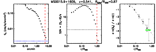
Figure 4: From left to right: (i) Chandra surface brightness profile of MS0015.9 with the fitted background (horizontal dotted line) and the radius $r_{200}$ (vertical dashed line); (ii) signal-to-noise profile, evaluated as $S2N=(S_{\rm X}-B)/\epsilon$ as function of $r/r_{200}$, where the error $\epsilon$ is the sum in quadrature of the Poissonian error in the radial counts and the uncertainties in the fitted background, $B$, defined by considering a region far from the X-ray center that covered a significant portion of the exposed CCD with negligible cluster emission; (iii) the best-fit values of the slope of the surface brightness profiles as a function of $r/r_{200}$. The thick horizontal solid line indicates the slope evaluated between $0.4$ $r_{200}$ and $R_{S2N}$ with a minimum of 3 radial bins. The dashed line indicates the best-fit of $d\ln(S_{\rm X})/d\ln(r/r_{200})$ with the functional form $s_{0}+s_{1}\ln(r/r_{200})$ over the radial range $0.1$ $r_{200}$–$R_{S2N}$ (reprinted with permission from Ettori & Balestra 2009).

Indeed, modelling cluster outskirts with hydrodynamical simulations is generally considered an easier task with respect to cluster cores. The reason is that any form of feedback effect is usually connected with active galactic nuclei (AGN) and star-formation and, therefore, with gas density, thus leaving the external regions more dominated by gravitational collapse. In fact, it has been shown with hydrodynamical simulations that different physical prescriptions have a small impact on clusters’ profiles in the outskirts. Roncarelli et al. (2006, see also Fig. 1) studied the behavior of the profiles of density, temperature and surface brightness in a sample of 9 galaxy groups and clusters simulated with the Lagrangian code GADGET-2, with non-radiative physics and with several treatments of cooling, star-formation, feedback, viscosity, and thermal conduction. They found a clear steepening of all the profiles around the virial radius with very small differences due to the physical models. In detail, the slope of the soft, (0.5–2) keV, X-ray surface brightness changes from about $-3.2$ close to the center to about $-5.5$ in the outskirts for high-mass objects, with a slope of $-4,-4.5,-5.2$ when estimated in the radial range (0.3–1.2) $r_{200}$, (0.7–1.2) $r_{200}$, (1.2–2.7) $r_{200}$, respectively, in excellent agreement with the observational constraints. Moreover, on the scale of galaxy groups ($M_{200}\sim 10^{14}M_{\odot}$), the steepening is much more prominent, with slopes that vary from about $-2.5$ to $-7.5$. A similar behavior is measured in the profiles of the gas density and temperature. These evidences can be explained as due to the fact that, in the present scenario for structure formation, galaxy groups are dynamically older and more relaxed than clusters, as also suggested from the observed and simulated behavior of the concentration–mass relation (e.g., Neto et al., 2007; Buote et al., 2007; Ettori et al., 2010).

However, simulations highlight that the accretion pattern in the outskirts is indeed complicated. Non-adiabatic effects like turbulence and shocks are frequent in unrelaxed systems and can influence the pressure profiles. Even if these processes are not connected to any feedback of the star-forming phase, they often require special treatment in the simulations because they act at small scales that are difficult to reach in cosmological simulations. Recently, Vazza et al. (2009) ran simulations with the Eulerian adaptive mesh refinement (AMR) code ENZO including the implementation of a new sub-grid refining scheme, allowing them to study the velocity pattern of the ICM in simulated clusters. Their results showed that the kinetic and turbulent energy associated with the ICM account for 5–25 per cent of the total thermal energy inside $r_{\rm vir}$. Burns et al. (2010) found a remarkable agreement between the temperature, density, and entropy profiles of 24 mostly substructure-free massive clusters simulated with the ENZO code and the published Suzaku results, implying that (i) the simplest adiabatic gas physics is adequate to model the cluster outskirts without requiring other mechanisms (e.g., non-gravitational heating, cooling, magnetic fields, or cosmic rays), and (ii) the outer regions of the ICM are not in hydrostatic equilibrium.

Inhomogeneities in the X-ray emission due to random density fluctuations are expected. Using simulated clusters, Mathiesen et al. (1999) measured a mean mass-weighted clumping factor $C=\langle\rho_{\rm gas}^{2}\rangle/\langle\rho_{\rm gas}\rangle^{2}$ between 1.3 and 1.4 within a density contrast of 500. If clumping is ignored, the gas density, and therefore, the gas mass, gets overestimated by $\sqrt{C}$. Nagai & Lau (2011) analysed 16 simulated clusters and computed their clumpiness profiles with and without radiative cooling. They found that, at $r_{200}$, $C$ goes from 1.3 in the former to 2 in the latter ones. The non-radiative clumping factor is higher because radiative cooling removes gas from the hot $T>10^{6}$ K X-ray emitting phase in the simulations. This shows that adding gas physics has quite a significant effect in cluster outskirts. The authors suggest that, since hydrodynamical simulations suffer of a form of overcooling problem, the true result is likely to be between these values. Overall, they concluded that gas clumping leads to an overestimate of the observed gas density and causes flattening of the entropy profile, as suggested qualitatively from recent Suzaku observations (e.g., Hoshino et al., 2010; Simionescu et al., 2011).

Suzaku has indeed improved the observational characterization of the faint emission from cluster outskirts, providing the first spectroscopic constraints on it (Section 4.1.2). Simionescu et al. (2011) have resolved the baryonic and metal content of the ICM in the Perseus cluster out to $r_{200}\sim 1.8h_{70}^{-1}$ Mpc, estimating a clear excess of the gas fraction with respect to the expected cosmic value along the northwest axis, and confirming some preliminary evidence from ROSAT PSPC (Ettori et al. 1998, where the gas density is resolved at $r_{200}$ but an isothermal gas is assumed due to limited spectral capability of the PSPC; see Fig. 5). They suggest that clumpiness of the ICM on the order of $C\approx$ 4–16 over the radial range (0.7–1) $r_{200}$ is required to properly reconcile the expected and measured gas mass fraction; i.e., significantly higher $C$ than indicated by the simulations described above.

Figure 5: Left (from Simionescu et al. 2011, reprinted with permission from AAAS): Deprojected electron density, entropy ($K$), and pressure profiles towards the northwest (red data points) and east (blue data points) of the Perseus cluster, measured with Suzaku. The red line shows the northwestern profiles corrected for clumping. The expected entropy profile from simulations of gravitational collapse (Voit, 2005) is a power-law with index 1.1 over-plotted in the entropy panel (black dotted line). The average profile of a sample of clusters previously studied with XMM-Newton within $\sim$0.5 $r_{200}$ (Arnaud et al., 2010) is shown in the pressure panel (solid black curve; its extrapolation to $r_{200}$ is shown with a dotted black line). Right (from Ettori et al. 1998, reprinted with permission): Gas mass fraction profiles obtained from the deprojection of the ROSAT PSPC surface brightness profiles in different azimuthal sectors by assuming a Navarro-Frenk-White (NFW) dark matter density profile (triangles joined by a dotted line). The gas fraction measured from the azimuthally averaged profile, both using an isothermal profile (solid line) and an NFW profile (dashed line), is shown. $r_{200}=2.7$ Mpc in this analysis. An Einstein-de Sitter Universe with $H_{0}=50$ km s^-1 Mpc^-1 is here adopted.

A more observable quantity is the estimate of the azimuthal scatter along the cluster radius $S(r)=\sqrt{1/N\,\sum_{i}\frac{\left[y_{i}(r)-Y(r)\right]^{2}}{Y(r)^{2}}}$, where $y_{i}(r)$ is the radial profile of a given quantity, taken inside a given $i-$sector, and $Y(r)$ is the average profile taken from all the cluster volume. Contributions to this scatter are expected from both an intrinsic deviation with respect to the spherical symmetry and, most importantly, to the presence of filaments of X-ray emission associated to any preferential direction in the accretion pattern of the ICM.

Two sets of high-resolution cosmological re-simulations obtained with the codes ENZO and GADGET2 are used in Vazza et al. (2011) to show that, in general, the azimuthal scatter in the radial profiles of X-ray luminous galaxy clusters is about 10 per cent for gas density, temperature, and entropy inside $r_{200}$, and 25 per cent for X-ray luminosity for the same volume. These values generally double approaching 2 $r_{200}$ from the cluster center, and are found to be higher (by $\sim$20–40 per cent) in the case of perturbed systems. These results suggest the possibility to interpret the large azimuthal scatter of observables as estimated from, e.g., Suzaku with the present simulated data.

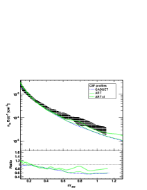
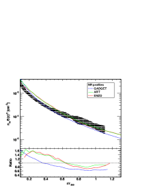
Figure 6: Comparison between the mean ROSAT density profile for a sample of 31 nearby X-ray bright galaxy clusters and numerical simulations both including cooling and star formation (left) and with non-radiative physics (center). Right: Stacked emission measure profile (in units of cm^-6 Mpc) for the entire sample (black), the cool-core (CC, red) and non-cool-core (NCC, blue) systems. The bottom panel shows the ratio between the CC and NCC populations. Reprinted with permission from Eckert et al. (2012).

In Eckert et al. (2012), a stacking analysis of the gas density profiles in a local ($z=$ 0.04–0.2) sample of 31 galaxy clusters observed with ROSAT PSPC is presented (Fig. 6). They observe a steepening of the density profiles beyond $\sim$$r_{500}$. They also report the high-confidence detection of a systematic difference between cool-core and non-cool-core clusters beyond $\sim$0.3 $r_{200}$, which is explained by a different distribution of the gas in the two classes. Beyond $r_{500}$, galaxy clusters deviate significantly from spherical symmetry, with only little differences between relaxed and disturbed systems. The observed and predicted (from numerical simulations) scatter profiles are in good agreement when the 1% densest clumps are filtered out in the simulations. While all the different sets of simulations used by them, especially beyond $\sim$0.7 $r_{200}$, show a relatively good agreement, they seem all to predict steeper profiles than the observed one from the PSPC, in particular in the radial range between 0.4 and 0.65 $r_{200}$. Approaching $r_{200}$, the slope increases up to $\beta\approx 1$ both in simulated and observed profiles. Eckert et al. also conclude that a slightly better agreement in terms of shape of the gas density profile is found when a treatment of the observational effects of gas clumping is adopted (as, e.g., in Nagai & Lau 2011).

At very large radii up to $r_{\rm vir}$, Suzaku data seem to indicate a flattening of the gas density profile (e.g., Kawaharada et al., 2010). Recall (eq. 6) that the gas density gradient enters linearly in the total mass determination. A flatter profile, therefore, results in a lower total mass estimate (and a larger gas mass estimate).

4.1.2 Temperature profiles

We have seen (e.g., Fig. 3) that the inferred total cluster mass strongly depends on the measured temperature profile. This is mostly because $T_{\rm gas}(r)$ enters linearly in the hydrostatic equation (6), therefore, a 20% uncertainty in $T_{\rm gas}(r)$ results in a mass uncertainty contribution of 20% if a fixed radius is chosen ($\sim$30% if the mass is determined within an overdensity radius).

Despite the poor, energy-dependent point-spread-function (PSF), the Advanced Satellite for Cosmology and Astrophysics (ASCA) provided temperature profiles to large radius for some clusters (e.g., Markevitch et al., 1996; Fukazawa, 1997; Markevitch et al., 1998; White, 2000), as well as BeppoSAX (e.g., Irwin et al., 1999; Irwin & Bregman, 2000; De Grandi & Molendi, 2002). Due to their high particle backgrounds, XMM-Newton and Chandra usually cannot robustly reach the cluster outskirts (e.g., Allen et al., 2001; Zhang et al., 2004; Vikhlinin et al., 2005; Arnaud et al., 2005; Kotov & Vikhlinin, 2005; Piffaretti et al., 2005; Pratt et al., 2007; Snowden et al., 2008; Leccardi & Molendi, 2008b), apart from a few special, e.g., very bright, low temperature, systems (e.g., Urban et al., 2011; Bonamente et al., 2013).

The breakthrough came recently after the launch of Suzaku, a satellite in low-Earth orbit and with short focal length (Mitsuda et al., 2007), resulting in a low and stable particle background. The first Suzaku temperature measurements reaching beyond the XMM-Newton and Chandra limit were published by Fujita et al. (2008a); Reiprich et al. (2009); George et al. (2009); Bautz et al. (2009). The latter three are all based on relaxed cool-core clusters, while Fujita et al. (2008a) targeted the compressed and heated interaction region between A399 and A401 with the primary goal to constrain the metallicity (Section 5). While initially there were sometimes difficulties to properly account for all fore- and background components (see the technical Section 6.1.1 for details on these components), especially for clusters at low Galactic latitude (George et al., 2009; Eckert et al., 2011), more elaborate robust analyses are now routinely being performed (e.g., Walker et al., 2012a).

The $\sim$100 refereed articles that are turned up by ADS when searching for “Suzaku” and “cluster” in the abstract have already received $>$1,000 citations at the time of writing (December 2012), demonstrating the large interest in Suzaku cluster studies. The six most highly cited references of these all deal with cluster outskirts, which shows that this interest is driven particularly by this subject.

Figure 7: All published Suzaku temperature profiles that reach cluster outskirts. The references are listed in the text.

In Fig. 7 all currently available Suzaku cluster temperature profiles are shown that reach beyond about 1/2 $r_{200}$ (to our knowledge; see also Akamatsu et al. 2011 for an earlier compilation). The purpose of this compilation is to test for similarities of the temperature profiles and, if similar, to determine the general trend and compare to predicted profiles. Before proceeding however, a few words of caution are in order: While the Arnaud et al. (2005) $\langle k_{\rm B}T\rangle$–$r_{200}$ relation (for their hot cluster subsample, assuming a flat Universe with $H_{0}=71$ km/s/Mpc and $\Omega_{\rm m}=0.27$) was used homogeneously for all clusters for the radial scaling, the shown data are inhomogeneous in several other aspects. These include, e.g., background subtraction, PSF correction, deprojection, $\langle k_{\rm B}T\rangle$ determination, and radial bin center calculation, so this will cause increased dispersion in the profiles. Also, both axes are not completely independent since both are scaled by $\langle k_{\rm B}T\rangle$ ($\langle k_{\rm B}T\rangle^{1/2}$ for $r_{200}$), which further increases dispersion (due to the negative slope of the profiles). So, even if the true scaled cluster temperature profiles were perfectly self-similar, we expect to see dispersion in Fig. 7.

The vertical bars shown are the 68% confidence level statistical uncertainties. Some authors provided also total systematic uncertainties. Typically, in the outer parts, they are of roughly similar size as the statistical errors. The horizontal bars indicate the radial range used for accumulating the spectra.

The authors were asked to flag their clusters or azimuthal directions as either “relaxed” or “merging.” In Fig. 8 both sets of profiles are compared (without error bars, for clarity). While there appears to be more scatter in the profiles of the clusters flagged as merging, this is mostly due to A3376 and A2804. In the merging cluster A3376, Akamatsu et al. (2012b) clearly identified a shock front, which can be appreciated in Fig. 8 (right) as the profile with a maximum around (0.7–0.8) $r_{200}$. A2804 is a group that lies between two hotter clusters (Sato et al., 2010), which seems to cause an untypically flat temperature profile in the outer parts (second highest relative temperature at $\sim$0.8 $r_{200}$). Overall, the trends of the relaxed and merging profiles are rather similar and in Fig. 9 all profiles are therefore combined, excluding only those of A3376 and A2804.

Figure 8: Suzaku temperature profiles of clusters flagged as relaxed (left) and merging (right).

In the inner region ($\lesssim$ 0.3 $r_{200}$) the profiles appear flat. This is due to the large spread and radially varying slopes of central temperature profiles as observed with Chandra and XMM-Newton (e.g., Vikhlinin et al., 2005; Pratt et al., 2007; Hudson et al., 2010) combined with Suzaku’s broad PSF. Beyond this central region, temperatures systematically decline by a factor of about three out to $r_{200}$ and slightly beyond.

The Suzaku average profile is compared to profiles predicted by $N$-body plus hydrodynamic simulations (Roncarelli et al., 2006; Nagai et al., 2007a; Burns et al., 2010; Vazza et al., 2011), employing different numerical algorithms and incorporating different physics (Fig. 9, right). Before proceeding, it needs to be stressed that this comparison should not be overinterpreted. This is, on the one hand, because the simulations vary in several aspects, e.g., they employ different temperature definitions. Moreover, all simulations have difficulties reproducing the temperature structure in cluster cores as observed by Chandra and XMM-Newton. Results in cores depend strongly on the additional physics put in. The point is now that the profiles in Fig. 9 are normalized by some average temperature ($\langle k_{\rm B}T\rangle$), which depends also on the temperature structure in the core. We have, therefore, increased $\langle k_{\rm B}T\rangle$ by 50% for the Roncarelli et al. (2006) and Vazza et al. (2011) profiles in order to roughly renormalize them to fit the cluster outskirts, as many authors find that employing different physics recipes does not affect much the outer temperature profiles. Without this rescaling, the Roncarelli et al. and Vazza et al. profiles would lie above the two other simulated profiles.

In any case, the slopes of observed and simulated temperature profiles appear consistent in the outskirts; if anything, then the observed average temperature profile drops off slightly faster than the simulated ones at the largest radii, as already noted in the very first Suzaku temperature profile determination of a relaxed cluster (Reiprich et al., 2009). In Fig. 9 (right), this is illustrated by the dashed line, which gives the best linear fit to the data points in the range $0.3r_{200}<r<1.15r_{200}$ as $k_{\rm B}T/\langle k_{\rm B}T\rangle=1.19-0.84r/r_{200}$.

Figure 9: All Suzaku temperature profiles, excluding A3376 and A2804 (see text; left: individual profiles, right: binned average profile). 162 temperature measurements are binned into 18 radial bins, each containing 9 temperature measurements. Error bars denote the standard deviation of temperature measurements in each bin. Also shown are (partially renormalized, see text) average temperature profiles from numerically simulated clusters from Roncarelli et al. (2006); Nagai et al. (2007a); Burns et al. (2010); Vazza et al. (2011). The dashed line represents a simple linear fit to the data points beyond 0.3$r_{200}$.

It has already been mentioned that some authors provided more than one Suzaku temperature profile for a given cluster by subdividing the profile into azimuthal directions, sometimes finding significant differences. For instance, Kawaharada et al. (2010) found that in the northeastern direction of Abell 1689 the temperature around the virial radius is about three times larger than temperatures in other directions. Moreover, they found this enhanced temperature to be correlated with a large-scale structure filament in the galaxy distribution and argue that thermalization is faster in this overdense infall region.

So, with Suzaku we have been moving forward, temperature measurements out to $\sim$$r_{200}$ can be performed and we expect more progress in the next few years through homogeneous sample studies with Suzaku and the upcoming eROSITA and Astro-H (e.g., Takahashi et al., 2012) instruments, the latter satellite also carrying a high spectral resolution micro-calorimeter array (e.g., Mitsuda et al., 2012). Nevertheless, we are still quite far away from the outer border of cluster outskirts according to our definition (3$r_{200}$, Section 2). New X-ray missions with low particle background, low soft proton contamination, good PSF for AGN removal, large field-of-view, and large effective area will likely be required to reach this frontier.

There is another route to constraining temperature profiles in cluster outskirts: the combination of X-ray surface brightness measurements with SZ decrement profiles (e.g., Basu et al., 2010). This will be discussed in more detail in Section 6.2. Naively speaking, the SZ effect depends on the gas density and the X-ray emission on the square of the density, therefore, the SZ signal might trace the low density cluster regions better than the X-ray signal. However, the actual situation is slightly less straightforward since the SZ signal also decreases linearly with decreasing temperature; i.e., in cluster outskirts (Fig. 9) while the soft X-ray emission increases with decreasing temperature for $k_{\rm B}T_{\rm e}\lesssim 2$ keV due to line emission (Fig. 2). So, overall, the relative gain in sensitivity of SZ measurements compared to X-ray measurements in cluster outskirts is not as strong as naively implied by the comparison of density dependencies.

4.1.3 Pressure profiles

As the main balance for gravitation in massive halos, the distribution of thermal pressure within the ICM is of particular interest. It has been investigated via X-ray observations. Work based on XMM-Newton observations of the REXCESS sample, a representative sample of nearby clusters (Böhringer et al., 2007; Pratt et al., 2009), has demonstrated that the scaled distribution of the ICM pressure follows a universal shape. The observational constraints extend out to a radius of $r_{500}$. Within this radial range, the observed pressure profiles are well-matched by predictions from various numerical simulations (Borgani et al., 2004; Nagai et al., 2007a; Piffaretti & Valdarnini, 2008). Without observational constraint beyond $r_{500}$, Arnaud et al. (2010) provided a simple “universal pressure profile” parametrisation of a generalized NFW (GNFW) function from the XMM-Newton data and the aforementioned numerical simulation (beyond $r_{500}$). This work has been extended down to the group regime by Sun et al. (2011) from Chandra data; see also, e.g., Finoguenov et al. (2007) for earlier work based on XMM-Newton.

Baryons in the outskirts bear the signature of the continuous three-dimensional non-spherical accretion from surrounding filaments. In this sense, access to the level of thermal pressure in the cluster outer parts provides a neat way to assess the virialization degree achieved, the thermodynamical state of the (pre-shocked) in-falling material (Voit et al., 2002, 2003), etc.

Observational constraints on cluster outskirts are sparse and difficult to gather, although these regions encompass most of the cluster volume. X-ray observations have recently provided a first insight out to $\sim$$r_{200}$ of the physical properties of the gas (Sections 4.1.1 and 4.1.2).

Figure 10: Both figures and caption reproduce content from Planck Collaboration et al. (2013), reprinted with permission. Refer to this paper for a description of the $f(M)$ factors. Left: Planck pressure profile obtained from the average of the individual pressure profiles across the sample (red points) shown together with the stacked pressure profile derived from the XMM-Newton data for the same sample (purple points). The dispersions about the SZ and X-ray profiles are depicted, respectively, by the red and purple shaded areas. The best-fit GNFW profile is shown as a solid black line and that of Arnaud et al. (2010) as a solid green line. The lower panel shows the $\chi$ profile of these two best-fit models taking into account the statistical errors and dispersion about the observed profile. Right: Measured pressure profiles from Planck and XMM-Newton. The three shaded areas mark the dispersions about the average profiles for three samples of simulated clusters: in blue, the simulations from Borgani et al. (2004), Nagai et al. (2007a) and Piffaretti & Valdarnini (2008), which were used in Arnaud et al. (2010) to derive the universal pressure profile together with the REXCESS data; in green, the simulated sample of clusters from Dolag et al. (in prep.); and in brown the simulated clusters from Battaglia et al. (2012). The corresponding average profiles for each set of simulations are plotted as solid lines using the same color scheme. In the bottom panel, the $\chi$ profiles between the observed profile and the simulated average profiles are presented, taking into account their associated dispersion.

The SZ effect has the potential to contribute greatly to the discussion on cluster outskirts due to its linear dependence on density and temperature. The radial pressure distributions of the first SZ cluster samples have recently been presented based on observations with, e.g., the SZ Array / Combined Array for Research in Millimeter-wave Astronomy (SZA/CARMA, Mroczkowski et al., 2009; Bonamente et al., 2012), APEX-SZ (Basu et al., 2010), and the South Pole Telescope (SPT, Plagge et al., 2010). These studies confirmed that the ICM properties as seen by SZ and X-ray observations are consistent at least out to $r_{500}$. Noticeably, Plagge et al. (2010) have obtained from 11 SPT clusters a stacked SZ profile out to $\sim$(1.5–2)$r_{500}$, where the shape of the underlying pressure profile is compatible with the one given by Arnaud et al. (2010).

A significant set of results has recently been published by the Planck Collaboration et al. (2013) based on the Planck nominal survey (i.e., 14 months of survey). Making use of its full sky coverage over nine frequency bands (Planck Collaboration et al., 2011a), the Planck satellite maps all cluster scales from its native resolution (5 to 10 arcmin at the SZ relevant frequencies) to their outermost radii, even for nearby clusters. The Planck Collaboration adopted a statistical approach to derive a stacked SZ profile from a sample of 62 nearby clusters detected in SZ with high significance. These clusters were selected from the Planck Early SZ (ESZ) sample and were previously used to investigate the total integrated SZ flux and the SZ scaling relations (Planck Collaboration et al., 2011c).

The statistical detection of the SZ signal extending out to 3$r_{500}$ provides the first stringent observational constraints on the ICM pressure out to a density contrast of $\delta\,{\sim}\,50$–100. Correcting for the instrument PSF and deprojecting the 2D profile into a 3D one, the Planck collaboration derived the underlying thermal pressure profile of the ICM. This observed pressure profile is in excellent agreement with the one derived from XMM-Newton archive data for all 62 clusters, over the overlapping radial range of (0.1–1)$r_{500}$. The combined SZ and X-ray pressure profile gives for the first time a comprehensive measurement of the distribution of thermal pressure support in clusters from 0.01$r_{500}$ out to 3$r_{500}$. Similarly to Arnaud et al. (2010), the Planck Collaboration has derived an analytical representation assuming a GNFW profile (as formulated by Nagai et al., 2007a) with best-fit parameters $[P_{0},c_{\rm 500},\gamma,\alpha,\beta]=[6.41,1.81,0.31,1.33,4.13]$ (Fig. 10), the outer slope ($\beta$) being slightly shallower than the extrapolation based on simulations that was used by Arnaud et al. (2010). Weak hints for even flatter outer slopes have been found recently with Bolocam data of a sample of 45 clusters (Sayers et al., 2012). In the inner parts, there seems to be some tension between the XMM-Newton data points and the Arnaud et al. (2010) XMM-Newton profile (although well within the dispersion). As discussed in Planck Collaboration et al. (2013), this is likely caused by differences in selection of the two samples (i.e., fraction of dynamically perturbed versus relaxed clusters).

The observed joint Planck and XMM-Newton pressure profile is also in agreement within errors and dispersion over the whole radial range with various sets of simulated clusters (Borgani et al. 2004; Nagai et al. 2007a; Piffaretti & Valdarnini 2008; Battaglia et al. 2010; Dolag et al. in prep.). Within the spread of predictions it matches best the numerical simulations that implement AGN feedback, and it presents a slightly flatter profile compared to most of the above theoretical expectations in the outerparts.

As outlined in Section 1, the physics at play in cluster outskirts is still to be understood. The constraints on gas pressure brought from the Planck stacked SZ measurements have shed light over a volume almost an order of magnitude larger than that accessible from X-ray data of individual clusters alone. Further SZ and X-ray measurements, especially for complete samples that are not subject to possible archive biases, will continue to provide an observational insight of cluster outskirts and serious constraints for theoretical studies on issues such as gas clumping, departures from hydrostatic equilibrium, contribution from non-thermal pressure, etc., as will be discussed in the following several Sections. SZ and X-ray measurements complement each other nicely in this sense since they primarily constrain different physical properties of the gas (SZ: pressure, X-ray: density and temperature).

4.1.4 Entropy profiles

Figure 11: Left: Scaled entropy profiles measured with Suzaku, apart from A1835 and A2204 (Chandra, black boxes and triangles, respectively) and Virgo (XMM-Newton, green crosses); compiled by Walker et al. (2012b, reproduced with permission). The black lines show the entropy profile and scatter as derived by combining the Planck average pressure profile (Fig. 10) with the ROSAT average density profile (Fig. 6). The straight line represents an $r^{1.1}$ power-law normalized to 1 at 0.3$r_{200}$. Right: Scaled entropy profiles determined by Eckert et al. (2013b, reproduced with permission). The straight dotted line again has a slope of $r^{1.1}$ but is normalized using the definition of Voit (2005). For the green band and the red triangles, the same data (average Planck and ROSAT profiles) as on the left are used. The two symbols represent different analysis methods (density determination through fitting a function to the emission measure profile and through direct deprojection, respectively). Also shown (circles) are the results from determining individual entropy profiles for 18 clusters in common between the Planck and ROSAT samples.

Often, “entropy” is defined in this field as $K\equiv k_{\rm B}T_{\rm gas}/n_{\rm e}^{2/3}$; i.e., the discussion can be kept short here since it can basically be derived by combining Section 4.1.1 (density profiles) either with Section 4.1.2 (temperature profiles) or with Section 4.1.3 (pressure profiles, through $K=P_{\rm e}/n_{\rm e}^{5/3}$). Moreover, several aspects of entropy have already been addressed in Section 4.1.1.

Typically, the temperature profiles observed with Suzaku in cluster outskirts tend to be fairly steep while the density profiles are often found to be less steep than expected (in particular for Suzaku). This results in a flatter slope compared to the expected entropy profile gradient $K\propto r^{1.1}$ (e.g., Voit, 2005) but note also exceptions to this, e.g., the fossil group RXJ1159+5531 (Humphrey et al., 2012). This is illustrated in Fig. 11 where the Suzaku data on the left show a clear drop off at large radii while this is much less obvious from the results on the right, possibly due to systematic differences between ROSAT and Suzaku density profiles, different chosen normalizations for the $r^{1.1}$ power-law, or differences in sample selection. Additionally, a possible difference in the way how the very same ROSAT (Eckert et al., 2012) and Planck (Planck Collaboration et al., 2013) data are combined in both works is suggested by the presence (absence) of non-monotonicity in the average profiles on the left (right). Interpretations also vary; while Eckert et al. (2013b) argue that the well-known central entropy excess extends out further than previously thought, Walker et al. (2012b) suggest that clumping in cluster outskirts could be one (but not the only) important effect. Since this review is concerned with cluster outskirts, we discuss clumping and several other possible physical and technical explanations in upcoming Sections, mostly in terms of effects on temperature and density measurements because the primary focus of this review is on mass profiles in cluster outskirts.

4.1.5 Gas/baryon mass fraction

The gas fraction, $f_{\rm g}\equiv M_{\rm gas}/M_{\rm tot}$, in clusters typically increases as a function of both mass and radius (e.g., Vikhlinin et al. 2006; see Section 7.4 in Reiprich 2001 for a discussion of pre-XMM-Newton and -Chandra results). Going out far enough into the outskirts, the cosmic mean baryon fraction, e.g., as determined from measurements of the cosmic microwave background radiation or the primordial deuterium-to-hydrogen-ratio, should eventually be recovered. It would be interesting to measure the characteristic radius at which this usually happens because this would help constrain the physical processes relevant for depleting the inner cluster regions of baryons. Moreover, cosmological applications involving the gas or baryon fraction of clusters rely on precise estimates of the gas/baryon depletion factor at a given radius and redshift (e.g., Ettori et al., 2009; Allen et al., 2011).

As discussed in Section 4.1.1, ROSAT and Chandra data as well as hydrodynamic simulations mostly indicate a steepening of the gas density profile with increasing radius up to $\sim$$r_{500}$ and beyond, while even further out, Suzaku data seem to favor a flattening. Taken at face value, gas mass fractions in excess of the cosmic mean baryon fraction are sometimes implied. On the other hand, many different physical effects, considered in the following Sections, could result in an artificial trend by affecting either the gas mass or total mass determination or both. Also, some challenges for measurements are outlined in the technical Section 6.1.

The ROSAT PSPC was great for measuring gas density profiles out to very large radius (e.g., Eckert et al., 2012, 2013a) because of the very low particle background level and large field-of-view. For instance, Reiprich (2001) measured the gas mass fraction within $r_{200}$ for 106 clusters. For 58 out of these clusters, only a small or no extrapolation of the measured surface brightness profile was necessary. The resulting $f_{{\rm gas},200}$ histogram is shown in Fig. 12. One notes that the Perseus cluster, a prominent example for a high Suzaku gas mass fraction and discussed in terms of gas clumping in Section 4.1.1, has one of the highest observed gas mass fractions of all 58 clusters ($f_{{\rm gas},200}=0.21$, in excellent agreement with the Suzaku measurement). While the statistical and systematic uncertainties of the total mass measurements are large, resulting in a broadening and possibly a shift of the distribution in Fig. 12, this could be an indication that the Perseus cluster just happens to lie on the extreme tail of the intrinsic cluster $f_{{\rm gas},200}$ distribution. Note that while the intrinsic dispersion of the $f_{{\rm gas},2500}$ distribution is small (for relaxed clusters, e.g., Allen et al., 2011) it may be larger for $f_{{\rm gas},200}$ (also considering the whole cluster population). Therefore, more Suzaku  (and Astro-H) and SZ observations of a complete sample of clusters may be required for a full understanding of the typical baryon fraction and possible gas clumping in cluster outskirts.

Figure 12: Gas mass fractions within $r_{200}$ based on ROSAT PSPC data. Values taken from Reiprich (2001) and converted to $H_{0}=70$ km/s/Mpc. Only those 58 clusters are shown for which significant cluster emission has been detected out to $r>0.8r_{200}$. The gas mass fraction of the Perseus cluster – in excellent agreement with the recent Suzaku measurement (Simionescu et al., 2011) – is marked with an arrow. WMAP9 data indicate a cosmic mean baryon fraction of around (16–17)% (Hinshaw et al., 2012).

4.2 Structure formation in action

Structure formation simulations show that galaxy clusters grow through mergers and infall of matter clumps along filaments (e.g., Borgani & Guzzo, 2001; Springel et al., 2005). Observational evidence of the former is widespread (e.g., Markevitch & Vikhlinin, 2007). Filamentary structures have also been seen for decades, e.g., in the galaxy and galaxy cluster distribution (e.g., Fig. 13).

Figure 13: Shown as yellow circles are $\sim$100 X-ray bright nearby galaxy clusters (Reiprich & Böhringer, 2002). The circle radii indicate the apparent $r_{200}$. In grey, the distribution of $\sim$0.5 million near-infrared selected local galaxies from 2MASS is shown (Jarrett et al., 2000). Both populations trace the same filamentary structure and superclusters. The reason one can see the same structures with a few X-ray galaxy clusters as with a much larger number of galaxies is that clusters are strongly biased tracers of the matter distribution; they are the lighthouses of structure in our Universe. Reprinted with permission from Reiprich et al. (2003).

The expected filamentary gas distribution between clusters; i.e., the WHIM, likely containing a significant fraction of all local baryons (e.g., Cen & Ostriker, 1999; Fukugita & Peebles, 2004), still evades a very significant robust detection in X-rays (e.g., Kaastra et al., 2003; Bregman & Lloyd-Davies, 2006; Nicastro et al., 2005; Williams et al., 2006; Rasmussen et al., 2007; Kaastra et al., 2006; Bregman, 2007; Buote et al., 2009). Significant progress has been made at UV wavelengths (tracing the lower temperature phase of the WHIM); see Kaastra et al. (2008) for detailed review articles on the WHIM, in particular Richter et al. (2008).

We are currently entering an era when the region between the well-observed cluster centers ($\lesssim r_{500}$) and the elusive WHIM ($\gtrsim 3r_{200}$) comes within reach of X-ray and SZ measurements (Section 4.1). This is a region where a lot of action related to structure formation is expected to be happening. For instance, Fig. 1 shows infalling clumps of matter. Typically, these higher density regions are predicted to have a cooler temperature than their surroundings. Observational confirmation is now needed to test this picture in detail. On the other hand, if these clumps are generally present but remain undetected, e.g., due to poor spatial resolution, they will bias the X-ray gas density and temperature measurements in the outskirts (this is described in Sections 4.1.1 and 4.6) and, unless they are in pressure equilibrium with the ambient gas, they will also bias interpretations of SZ measurements that assume a smooth distribution. So, quantifying differences of X-ray and SZ results may allow us to constrain unresolved clumping (e.g., Grego et al., 2001; Jia et al., 2008; Khedekar et al., 2013).

More action in outskirts related to structure formation includes, e.g., large Mach number accretion shocks and corresponding particle acceleration. While these phenomena may be traced through the non-thermal particle population in the radio, hard X-ray, and $\gamma$-ray bands (e.g., Pfrommer et al., 2008), also soft X-ray and SZ measurements are required for a full understanding of the overall plasma properties.

4.3 Hydrostatic equilibrium

In the following Sections, we will discuss a few (non-) equilibrium situations. For the X-ray and SZ mass determination, it is perhaps most straightforward to see that hydrostatic equilibrium is important since it is the basis for eq. (6).

For major cluster mergers, it is obvious that the assumption of hydrostatic equilibrium is not a good one. Moreover, simulations suggest that also in less disturbed clusters, turbulence and bulk motions, e.g., due to infalling clumps, may disrupt hydrostatic equilibrium at some level (e.g., Nagai et al., 2007b). This appears to be more significant the further out one goes in terms of fraction of overdensity radius (e.g., Lau et al., 2009; Meneghetti et al., 2010). See also Suto et al. (2013) for an alternative interpretation of hydrostatic equilibrium biases as acceleration term in the Euler equations.

Observationally, direct measurements of/upper limits on ICM turbulent velocites and bulk motions are currently limited to cluster cores or to merging subclusters (e.g., Sanders et al. 2011, using the XMM-Newton Reflection Grating Spectrometer (RGS); Sato et al. 2008; Sugawara et al. 2009; Tamura et al. 2011, using Suzaku CCDs). Claims of an observational detection of such motions in the Centaurus cluster have been made using ASCA and Chandra data (Dupke & Bregman, 2001, 2005, 2006) and refuted (Ota et al., 2007) using Suzaku data. A robust direct measurement of turbulence may need to await future X-ray missions, like the upcoming Astro-H carrying high spectral resolution micro-calorimeter arrays (e.g., Zhuravleva et al., 2012). To reach cluster outskirts, even larger effective areas will be required, possibly provided through an envisaged Athena-like mission (e.g., Barcons et al., 2012; Nevalainen, 2013).

In cluster centers, gas “sloshing” is widespread, resulting in spiral-like patterns in the surface brightness distribution (e.g., Markevitch & Vikhlinin, 2007, for a review). It has been suggested based on ROSAT, XMM-Newton, and Suzaku observations of the Perseus cluster that features produced by such motions could extend even out to radii approaching the virial radius (Simionescu et al., 2012).

Another highly sensitive probe of the physical state of the ICM in cluster outskirts, in particular turbulent pressure support in high-$z$ ($z\gtrsim 0.5$) objects, can be through the Sunyaev-Zel’dovich effect angular power spectrum, which is the integrated signal from all the unresolved clusters in the sky (Komatsu & Kitayama, 1999; Komatsu & Seljak, 2002). The SZ power spectrum is measured as a foreground component of the CMB signal with the same spectral dependence as the SZ effect. Half of the SZ power comes from low-mass clusters and groups ($M_{200}<2\times 10^{14}M_{\odot}$), and half of it also comes from high-redshift ($z>0.5$) systems (Komatsu & Seljak, 2002). Therefore, SZ power might provide the only method to study these otherwise un-observable systems with low mass and high redshift, although only through their summed contributions.

Unlike X-ray brightness, the integrated SZ signal of a cluster carries a significant weight from the volume outside of $r_{500}$, so the prediction of SZ power is strongly dependent on the pressure profile in the outskirts. The difficulty lies in detecting the SZ power itself, which is not the dominant source of foreground anisotropy at any frequency or angular scale. Recent SPT measurements have constrained the tSZ power at a low amplitude: $3.5\pm 1.0$ $\mu\mathrm{K}^{2}$ at ${\ell}=3000$ (Shirokoff et al., 2011). This is lower than the prediction from X-ray derived cluster pressure models (Shaw et al., 2010; Efstathiou & Migliaccio, 2012), but the difference can be the result of many different effects, like pressure support from gas bulk motions, AGN and star-formation feedback, or other non self-similar evolution of the ICM. Future CMB measurements with better frequency coverage and angular resolutions are expected to place a tighter constraint on the thermal SZ power and break some of these degeneracies. The cosmology dependence of the SZ power can also be nailed down by other methods, for example an accurate value of $\sigma_{8}$ will reduce its degeneracy with the uncertain gas physics.

Another possible, indirect route to determining how strongly X-ray and SZ hydrostatic mass determinations are affected by turbulence, bulk motions, and other gas physics effects is through comparison to weak lensing measurements, which do not rely on the assumption of hydrostatic equilibrium, in principle. This has been done extensively for the inner parts of clusters ($\lesssim$$r_{500}$, e.g., Ettori et al. and Hoekstra et al., this volume, for reviews) and it may be feasible now also for cluster outskirts, although also the weak lensing mass reconstruction accuracy is more limited in the outer parts (e.g., Section 6.3.1).

In addition to merger- or accretion-induced bulk motions, also convection may occur in the ICM. While a gas temperature gradient in itself does not imply a violation of hydrostatic equilibrium, convection should occur if the specific entropy decreases significantly with increasing radius (for a non-magnetic ICM, e.g., Landau & Lifschitz, 1991; Sarazin, 1986, Sections 4 and V.D.6, respectively); i.e., if

$$\frac{{\rm d}s}{{\rm d}r}<0\,.$$ (9)

With

$$s\propto\ln\frac{T_{\rm gas}}{\rho_{\rm gas}^{\gamma-1}}\,$$ (10)

and $\gamma=5/3$ this condition becomes

$$-\frac{{\rm d}\ln T_{\rm gas}}{{\rm d}r}>-\frac{2}{3}\frac{{\rm d}\ln\rho_{\rm gas}}{{\rm d}r}\,.$$ (11)

Typically, density gradients in clusters are much steeper than temperature gradients; so, generally no convection is expected. However, in cluster outskirts, there are some indications that density profiles may flatten (Section 4.1.1), temperature profiles may steepen (Section 4.1.2), and entropy profiles may turn over (Section 4.1.4). For instance, convectional instability was considered early on for A2163 by Markevitch et al. (1996). In the presence of magnetic fields, however, the situation may be more complex due to other possible instabilities, in particular the magnetothermal instability (MTI, Balbus, 2000) and the heat-flux-driven buoyancy instability (HBI, Quataert, 2008).

4.4 Thermal equilibrium, $T_{\rm e}=T_{\rm gas}$?

With several tens of millions of degrees the ICM is hot. An important heating mechanism is shock heating, either in cluster mergers or when infalling gas passes through an accretion shock. The ICM consists of electrons and ions. Most of the ions are protons, so for simplicity we just use the term protons now. In an accretion shock, primarily protons should be heated since they carry most of the kinetic energy. After leaving the shock front, the time scales for protons and electrons to reach Maxwellian velocity distributions are short; i.e., they will both settle into thermal equilibrium quickly, albeit at different temperatures. The time scale is (Spitzer, 1956, eq. 5-26)

$$t_{\rm eq}(\mathrm{x,x})\approx 1.13\times 10^{7}\,\mathrm{yr}\,Z_{\mathrm{x}}^{-4}\left(\frac{m_{\mathrm{x}}}{m_{\rm p}}\right)^{1/2}\left(\frac{k_{\rm B}T_{\mathrm{x}}}{{\rm 10\,keV}}\right)^{\frac{3}{2}}\left(\frac{n_{\mathrm{x}}}{10^{-3}\,{\rm cm^{-3}}}\right)^{-1}\left(\frac{\ln{\Lambda_{\mathrm{x}}}}{40}\right)^{-1}\,,$$ (12)

where $Z_{\mathrm{x}}$ is the particle species charge, $m_{\mathrm{x}}$ its mass, $T_{\mathrm{x}}$ its temperature after reaching equilibrium, $n_{\mathrm{x}}$ its number density, and $\ln{\Lambda_{\mathrm{x}}}$ its Coulomb logarithm. So, in typical cluster regions, this is about $t_{\rm eq}(\mathrm{p,p})\approx$ 10 Myr for protons and for electrons about a factor of 43 faster,

$$t_{\rm eq}(\mathrm{e,e})\approx\left(\frac{m_{\rm e}}{m_{\rm p}}\right)^{1/2}t_{\rm eq}(\mathrm{p,p})\approx 2.64\times 10^{5}\,\mathrm{yr}\left(\frac{k_{\rm B}T_{\rm e}}{{\rm 10\,keV}}\right)^{\frac{3}{2}}\left(\frac{n_{\rm e}}{10^{-3}\,{\rm cm^{-3}}}\right)^{-1}\left(\frac{\ln{\Lambda_{\mathrm{e}}}}{40}\right)^{-1}\,.$$ (13)

If the electrons are indeed heated less efficiently in the shock than the protons, resulting in $T_{\rm e}<T_{\mathrm{p}}$ after equilibration, they will reach equilibrium even faster than implied by the square root of their mass ratios.

What takes longer then is raising the electron temperature to the proton temperature. Assuming this process proceeds primarily through Coulomb collisions, the corresponding equipartition time scale is very roughly a factor of 43 longer than the proton equilibration timescale,

$$t_{\rm eq}(\mathrm{e,p})\approx\left(\frac{m_{\rm e}}{m_{\rm p}}\right)^{-1/2}t_{\rm eq}(\mathrm{p,p})\,,$$ (14)

and is given by (Spitzer, 1956, eq. 5-31)

$$t_{\rm eq}(\mathrm{e,p})\approx 2.51\times 10^{8}\,\mathrm{yr}\left(\frac{k_{\rm B}T_{\rm e}}{{\rm 10\,keV}}\right)^{\frac{3}{2}}\left(\frac{n_{\rm p}}{10^{-3}\,{\rm cm^{-3}}}\right)^{-1}\left(\frac{\ln{\Lambda_{\mathrm{e}}}}{40}\right)^{-1}\left(1+\frac{T_{\mathrm{p}}}{T_{\rm e}}\frac{m_{\rm e}}{m_{\rm p}}\right)^{\frac{3}{2}}\,.$$ (15)

The last two factors are close to 1, so they are ignored in the following and we also assume $n_{\rm e}\approx 1.2n_{\rm p}$. In cluster outskirts, both ICM densities and temperatures are significantly lower than in the better observed inner regions. Since the densities drop much more quickly, the net effect is an increase of the equipartition timescale. It can come close to one Gyr or even more,

$$t_{\rm eq}(\mathrm{e,p})\approx 10^{9}\,\mathrm{yr}\left(\frac{k_{\rm B}T_{\rm e}}{{\rm 1\,keV}}\right)^{\frac{3}{2}}\left(\frac{n_{\rm e}}{10^{-5}\,{\rm cm^{-3}}}\right)^{-1}\,.$$ (16)

So, there the X-ray-emitting electrons may have a cooler temperature than the invisible protons, resulting in a steeper X-ray temperature gradient towards the outskirts and, therefore, an underestimate of the total mass (Fig. 3).

The thermal equilibrium/equipartition situation in cluster mergers and cluster outskirts/WHIM has been studied theoretically by many authors (e.g., Fox & Loeb, 1997; Chieze et al., 1998; Ettori & Fabian, 1998; Takizawa, 1998, 1999; Courty & Alimi, 2004; Yoshida et al., 2005; Rudd & Nagai, 2009; Wong & Sarazin, 2009; Wong et al., 2010). It is worth mentioning that the situation may differ between merger shocks (small Mach numbers) and accretion shocks (large Mach numbers): the electron heating efficiency (relative to the one for protons) in a shock may be anticorrelated to the Mach number squared (Ghavamian et al., 2007) if other processes in addition to pure Coloumb heating are considered, resulting in fast relative electron heating in merger shocks and slow heating in accretion shocks. Indeed, for the textbook merger shock in the bullet cluster, the equipartition time scale seems about a factor of five shorter than implied by eq. (15) (Markevitch & Vikhlinin, 2007) assuming the Chandra lower temperature limits from Markevitch (2006) for the extremely hot post-shock gas to be robust against systematic calibration uncertainties.

Observational results have also been obtained for cluster outskirt measurements. For instance, the early ASCA work on Abell 2163 by Markevitch et al. (1996) triggered some of the theoretical studies mentioned above. More recently, Suzaku data have been used to constrain the equipartition state (e.g., Hoshino et al., 2010; Akamatsu et al., 2011). With current instruments, no strong direct constraints have been achieved, though.

Fig. 2 of Rudd & Nagai (2009) implies that for unrelaxed and relaxed clusters of similar temperature, the electron temperature in the outskirts deviates more strongly from the ion temperature for unrelaxed clusters. Naively, one might conclude from the similarity of Suzaku profiles (Fig. 8) that no such trend is observed; i.e., no strong evidence for significant non-equipartition. However, a proper comparison would need to account for the possible difference of intrinsic temperature profiles between relaxed und unrelaxed clusters, for the inhomogeneous definitions used to classify clusters as un-/relaxed, and, since the equipartition timescale depends on temperature (eq. 16), for the possible difference in the temperature distributions of the subsamples.

Since there are not only protons but also ions in the ICM, some of which are strong X-ray line emitters, there is hope to measure the ion temperature directly from the line width. This might be feasible with upcoming missions. For instance, the micro-calorimeter array aboard Astro-H will have an energy resolution of $<$7 eV (e.g., Takahashi et al., 2012), possibly just sufficient to detect a thermal broadening of $\sim$5 eV (e.g., Rebusco et al., 2008, in the absence of other more dominant line broadening effects like bulk motions and turbulence) but only in the X-ray bright central regions where the collisional equilibration time scale is shorter than the typical time since the last major merger in any case. An Athena-like mission could have enough effective area and energy resolution to measure the thermal broadening in nearby cluster outskirts, where the ion and electron temperatures possibly deviate.

4.5 Ionization equilibrium, $T_{\rm X}=T_{\rm e}$?

A very rough timescale for an astrophysical plasma to reach collisional ionization equilibrium (CIE) is given by

$$t_{\rm ion-eq}\approx 10^{12}\,{\rm s}\left(\frac{n_{\rm e}}{{\rm cm^{-3}}}\right)^{-1}$$ (17)

with some dependence on the considered element and temperature (Smith & Hughes, 2010). Most ions in the ICM are not in an excited state because radiative deexcitation is very fast.

Recasting (17) into units typical of cluster outskirts yields

$$t_{\rm ion-eq}\approx 3\times 10^{9}\,{\rm yr}\left(\frac{n_{\rm e}}{10^{-5}\,{\rm cm^{-3}}}\right)^{-1}\,.$$ (18)

Therefore, on the order of a Gyr may be required in cluster outskirts – long enough to possibly result in an important, measureable effect for some clusters.

Figure 14: Model spectra of 1 keV (left) and 5 keV (right) plasmas for different values of the ionization timescale. Black: $\tau=8\times 10^{10}$ s/cm³, red: $\tau=3\times 10^{11}$ s/cm³, green: $\tau=8\times 10^{11}$ s/cm³, and blue: $\tau=3\times 10^{12}$ s/cm³. The normalizations are scaled for visualization purposes. Other parameter values are $N_{\rm H}=3\times 10^{20}$ cm^-2, metal abundance = 0.2 solar, redshift = 0.1.

For a given temperature, how do plasma spectra differ depending on the ionization state? Fig. 14 shows that stronger low energy emission lines are present when the ICM has not yet achieved CIE ($\tau\lesssim 10^{12}$ s/cm³). In typical observed spectra with CCD-type energy resolution, this results in a shift of the peak position of the $\sim$1 keV emission line complex towards lower energies, especially for a low temperature plasma (Fig. 15). This indicates that one might obtain a biased temperature if one wrongly assumes CIE in the fitting process. Due to this shift, as illustrated in Fig. 17, a bias towards lower temperatures may then be expected. Indeed, this is the case as Fig. 16 (left) demonstrates. In the most extreme non-equilibrium ionization (NIE) cases simulated, temperatures are underestimated by a factor of $\sim$2.

Figure 15: Simulated Suzaku observations of a single-temperature ICM ($k_{\rm B}T=1$ keV) that is not fully in collisional ionization equilibrium (2,000–3,000 source photons). Black: $\tau=8\times 10^{10}$ s/cm³, red: $\tau=3\times 10^{11}$ s/cm³, and green: $\tau=3\times 10^{12}$ s/cm³.

Figure 16: Left: Best-fit temperatures when incorrectly assuming collisional ionization equilibrium as a function of $\tau$; for simulated Suzaku data, assuming temperatures of 1 keV and 5 keV. Other parameter values as in Fig. 14. Right: Metallicity bias under the same assumptions.

Since this bias, if present, will likely be larger for larger radius where the density is lower, it will translate into a too steep temperature profile, resulting in an underestimated total mass (Fig. 3).

In Section 5, the importance of cluster chemistry especially in outskirts is described. Here, we show in Fig. 16 (right) how the metal abundance determination is biased if CIE is assumed when it is not yet established. While there is no strong bias for low temperature clusters, the metallicity gets severely overestimated for hot clusters in the most extreme case ($\tau=8\times 10^{10}$ s/cm³). This is due to enhanced line emission in the NIE case.

Non-equilibrium ionization effects in low density plasmas have been studied theoretically in detail by several works (e.g., Yoshikawa & Sasaki, 2006; Akahori & Yoshikawa, 2010; Wong et al., 2011). Some authors have also tried to estimate these effects observationally (e.g., Fujita et al., 2008b; Finoguenov et al., 2010; Akamatsu et al., 2012a). Future high-spectral resolution instruments like the upcoming Astro-H or an envisaged Athena-like mission may be able to set tight constraints on ionization states in the outskirts of galaxy clusters and thereby constrain merger timescales.

4.6 How to disentangle multitemperature structure, $T_{\rm X}=T_{\rm e}$?

The widespread presence of temperature gradients in central (e.g., Allen et al., 2001; Hudson et al., 2010) and intermediate (e.g., Vikhlinin et al., 2005; Pratt et al., 2007) cluster regions, as well as in cluster outskirts (Section 4.1.2) shows that the ICM is not isothermal. Moreover, gas temperature maps show that even at a given radius, a wide distribution of temperatures can exist (e.g., Reiprich et al., 2004; Million & Allen, 2009; Randall et al., 2010; Lovisari et al., 2011), possibly depending on dynamical state (e.g., Zhang et al., 2009). Additionally, in cluster outskirts, emission from new matter infalling along filaments and possible cooler clumps might become more important (Fig. 1).

Therefore, in a given spectral extraction region (say, an annulus in cluster outskirts), emission from gas at multiple temperatures may be present. The data quality (e.g., number of source photons, signal-to-noise ratio, energy resolution) on the other hand may not be sufficient to constrain a multitemperature model. A single temperature model will then have to be fitted to the multitemperature spectrum. What will the best-fit temperature be? It has been shown that the answer depends on the used X-ray mirror/filter/detector system (e.g., Mathiesen & Evrard, 2001; Mazzotta et al., 2004; Rasia et al., 2005; Vikhlinin, 2006). This is easy to understand: the electron temperature, $T_{\rm e}$, is usually estimated from fitting a model, convolved with the instrumental response, to an observed spectrum. The most temperature-sensitive features in an observed spectrum with CCD-like energy resolution are (recall Fig. 2) the exponential bremsstrahlung cutoff at high energies, the slope of the bremsstrahlung emission at intermediate energies, and the location of the emission line complex at low energies (Fig. 17). An instrument with more effective area at low energies compared to high energies – relative to another instrument – is more sensitive to the low energy features and, therefore, will typically give rise to a lower single temperature estimate.

Figure 17: The low-energy emission line complex (predominantly Fe and O) as a function of the intracluster electron temperature assuming a metal abundance of 0.3 solar, a neutral hydrogen column density of $N_{\mathrm{H}}=3\times 10^{20}\ \mathrm{cm}^{-2}$, and a redshift of $z=0.05$. The energy resolution approximates that of current X-ray CCDs. All spectra assume the same electron density distribution. Notice how the emission peak shifts to higher energies for increasing temperatures, from orange (0.3 keV) to black (3 keV).

An illustration for the simple case of a two-temperature plasma is shown in Fig. 18 for Chandra, XMM-Newton, Suzaku, and eROSITA. Spectral data are simulated for these instruments assuming emission from plasma at two different temperatures (0.5 keV and 8 keV), with varying contributions (emission measure ratios – the x-axis) and assuming three different metallicities (0.3, 0.5, and 1 times solar) for the cooler component (the hotter component is always assumed to have a metallicity of 0.3 solar). Then single temperature (and single metallicity) models are fit to the simulated data and the best-fit temperatures are shown in the plots. The median values of 100 realizations are shown and the 68% errors are taken from the distributions. The values of parameters not shown are: hydrogen column density $N_{\rm H}=3\times 10^{20}$ cm^-2, redshift $z=0.1$, number of source photons $=10^{4}$, and the energy range used for fitting is (0.5–8.0) keV. For these illustrations, the source emission is assumed to dominate over the background at all energies, so no background is included in the simulations.

The plots show how the best-fit single temperature decreases with increasing emission measure ratio of cold and hot component (from 10% to equal emission measure). It also becomes clear how the temperature decreases with increasing metallicity because the number of low-energy photons constraining the fit increases in this case. Moreover, the plots clearly reflect the different sensitivities of the different instruments, e.g., the relatively hard Suzaku XIS-FI typically returns much higher temperatures than the relatively soft eROSITA.

Figure 18: Best-fit single temperature of two-temperature plasma emission as a function of emission measure ratio of the two components, for different X-ray instruments: Chandra ACIS-I (upper left), XMM-Newton EPIC-pn (upper right), Suzaku XIS-FI (lower left), and eROSITA (lower right). See text for details.

So, assuming increased multitemperature structure with increasing radius in cluster outskirts, e.g., due to infalling cold matter, eROSITA would see a steeper temperature gradient than Suzaku and, therefore, would give rise to a lower total mass estimate (Fig. 3) if the different temperature components cannot be spectrally disentangled.

This seems dramatic; however, we have picked an extreme case ($k_{\rm B}T_{\mathrm{e,hot}}=8$ keV, $k_{\rm B}T_{\mathrm{e,cold}}=0.5$ keV) for illustration purposes. As long as at least one temperature component is cooler than about 1 keV, the reduced $\chi^{2}$ is actually quite bad ($>$1.5) in most cases (for $10^{4}$ source photons in the absence of any background); i.e., it is actually clear from the observed spectrum that a single temperature model is a bad fit. Only if both temperatures are above about 2 keV provides the single temperature model an acceptable fit. In the presence of significant background, however, acceptable fits can be obtained also for cooler components.

Fig. 19 illustrates that also the metallicity determination is biased if the presence of a multitemperature plasma is ignored. For instance, in case both components have a metallicity of 0.3 solar (the red data points), the resulting best-fit single component metallicty could be higher for the particular situation simulated here. For a more detailed discussion see, e.g., Buote (2000); Gastaldello et al. (2010).

Figure 19: Metallicity bias when assuming a single-temperature and single-metallicity emission while the true emission actually has two components. Simulated Suzaku data have been used.

Future instruments (e.g., the upcoming Astro-H and an envisaged Athena-like mission) will have enough collecting area and spectral resolution to better distinguish multitemperature structures spectrally. This will be crucial for a better understanding of the thermodynamics and chemistry especially in cluster outskirts.

4.7 Helium sedimentation

While potentially important for cluster (gas) mass estimates, this topic is likely more relevant for inner cluster regions; therefore, it is only briefly summarized here. More details can be found, e.g., in Ettori & Fabian (2006); Markevitch (2007); Peng & Nagai (2009); Bulbul et al. (2011), and references therein.

The mean particle weight, $\mu$, enters the hydrostatic equation (6); it is inversely proportional to the total mass, $M_{\rm tot}$. Since the overdensity radius also depends on $M_{\rm tot}$ (eq. 3), the effect on the mass of changing $\mu$ is amplified, resulting in a ($\sim$1.5 times) stronger dependence for masses determined within an overdensity radius, e.g. $M_{2500}$. On the other hand, to calculate the ICM mass, $M_{\rm gas}$, from the observed electron density distribution (eq. 7), the ratio $\frac{\rho_{\rm gas}}{n_{\rm e}m_{\rm p}}$ needs to be known. So, the composition of the ICM matters for both the $M_{\rm tot}$ and the $M_{\rm gas}$ determination.

While, e.g., an iron atom is more than ten times heavier than a helium atom, helium is about 10,000 times more abundant in typical ICM conditions than iron. Moreover, diffusion operates faster for lighter elements (e.g., Gilfanov & Sunyaev, 1984; Chuzhoy & Loeb, 2004). Therefore, the strongest influence on $\mu$ and $\frac{\rho_{\rm gas}}{n_{\rm e}m_{\rm p}}$ should come from variations in the helium-to-hydrogen ratio, $\frac{n_{\rm He}}{n_{\rm H}}$.

If a significant fraction of helium ions settled towards the cluster center over time, then $\frac{n_{\rm He}}{n_{\rm H}}$ would increase there. Hydrodynamic simulations indicate, an increase of the helium-to-hydrogen ratio of a factor of two might be realistic in some cases (e.g., Peng & Nagai 2009, with some dependence on the strength and structure of the cluster magnetic field and the temperature). Assuming $\frac{n_{\rm He}}{n_{\rm H}}=0.083$ and typical abundances of heavier elements, $\mu$ is approximately in the range 0.59–0.60, and $\frac{\rho_{\rm gas}}{n_{\rm e}m_{\rm p}}$ in the range 1.14–1.15. Doubling the helium-to-hydrogen ratio, one obtains about 0.67 and 1.25 for the same quantities, respectively. Neglecting helium sedimentation; i.e., assuming the wrong helium-to-hydrogen ratio (0.083), would in this case bias high $M_{\rm tot}$ by $\sim$13% and $M_{\rm gas}$ low by $\sim$8%, within a fixed radius. If these were the only effects, then the gas mass fraction, $f_{\rm g}\equiv M_{\rm gas}/M_{\rm tot}$, would be biased low by $\sim$19% compared to the true fraction.

However, there is another effect because, actually, only the X-ray flux is directly observed, not the electron number density. Since the emissivity (eq. 7) depends on the relative number of ions present, the flux to $n_{\rm e}$ conversion is affected by the assumed helium-to-hydrogen ratio. If the true helium-to-hydrogen ratio is higher by a factor of two than the assumed one then the electron density will be overestimated by about 5% when fitting a typical cluster spectrum (taking into account that the true electron-to-hydrogen ratio increases from about 1.17 to 1.33 when increasing the helium abundance).

Therefore, considering all three effects (underestimated $\mu$, underestimated $\frac{\rho_{\rm gas}}{n_{\rm e}m_{\rm p}}$, and overestimated $n_{\rm e}$), $f_{\rm g}$ might be very roughly underestimated by $\sim$14% in some cluster centers, given these very simplified assumptions. Since the true helium-to-hydrogen ratio in cluster centers is unknown, $f_{\rm g}$ might be best determined within large radii, approaching cluster outskirts, where the helium-to-hydrogen ratio should not be strongly affected by sedimentation. Combining X-ray, SZ, and gravitational lensing observations could, in principle, enable a measurement of the helium sedimentation factor. In particular, the SZ effect depends only on the electron density and not on the product of electron and ion density as the X-ray emission.

4.8 Gas clumping

Gas clumping; i.e., inhomogeneities in the gas distribution (and possibly the temperature distribution), must be present in the intracluster medium at some level. However, at which level, at what size scales, and how it varies with increasing distance from the cluster center is not very clear, yet. Observational and theoretical aspects of gas clumping have already been discussed in several previous Sections, including particularly Section 4.1.1. This will not be repeated here. In short, if present, the effect of increasing clumping with radius would be to overestimate the gas mass, because the gas density in a given region would be overestimated, and to underestimate the total mass, because the gas density profile would appear to drop less steeply (the total mass is proportional to the gas density gradient, eq. 6), and because the temperature profile may appear to drop more steeply if the clumps are cool (Fig. 3 shows that a larger gradient in temperature typically results in a lower total mass estimate). That is, each of the three effects would tend to result in an overestimated gas mass fraction.

If significant clumps are present at large-enough scales, they might be directly observed in deep X-ray surface brightness images (e.g., Vazza et al., 2013). Alternatively, if clumps are cool, they may be revealed through X-ray spectroscopy. Furthermore, comparison of X-ray and SZ-derived ICM profiles may put upper limits on the clumping factor (e.g., references in Section 4.2). Also, one may get constraints from considering whether the already existing slight tension between predicted and observed SZ angular power spectrum discussed in Section 4.3 might become more severe if significant gas clumping were present in cluster outskirts and resulted in an even more increased SZ signal.

5 Chemistry

5.1 Relevance of chemical evolution

Among the several outstanding problems of modern astrophysics, the chemical enrichment of the Universe is certainly a very topical one. In the standard scenario, shortly after the Big Bang, the element composition of the cosmic gas was very simple – it was composed almost entirely of hydrogen and helium, the two lightest chemical elements. Heavier elements than helium are thought to have their origin in the interiors and explosions of stars, which formed much later in the history of the Universe. It is believed that the first stars (“Population III”) formed few hundred million years after the Big Bang (e.g., Couchman & Rees 1986; Abel et al. 2002) from collapse of primordial, metal-free gas and they have subsequently polluted the surrounding medium by ejecting the metals produced in their cores (e.g., Galli & Palla 1998; Bromm et al. 1999; Yoshida et al. 2008; Cen & Riquelme 2008). The minimum amount of gas that may collapse under its own gravity is approximately given by the Jeans mass, which increases with temperature as $T^{3/2}$ (e.g., Bromm & Loeb, 2003). In a primordial environment, the only relevant coolants are H, He and their derived molecules (e.g., Saslaw & Zipoy 1967), which will not cool below a relatively high temperature of (100–200) K. Thus, the Population III stars are supposed to be more massive and short-lived (e.g., Woosley & Weaver 1995; Schaerer 2002) than the typical stars that form from metal-rich gas. Once the Population III stars had enriched the gas, cooling due to metal line emission became efficient and gas clouds could cool to lower temperatures and fragment into smaller pieces. The presence of metals probably drove the transition from a top-heavy initial mass function (IMF) to a ”Salpeter-like” IMF allowing low-mass stars to form.

5.2 Metallicity in cluster outskirts

The ICM does not only contain primordial elements, but also a considerable amount of heavy elements. As metals are only produced in stars, which reside mainly in galaxies, the enriched material must have been transported from the galaxies into the ICM. Several processes have been proposed to explain the observed enriched material: ram-pressure stripping, galactic winds, galaxy-galaxy interactions, AGN outflows, and intracluster stellar populations (see Schindler & Diaferio 2008 for a review). Each of them has a different efficiency and pattern distribution (e.g., Schindler et al. 2005; Domainko et al. 2006, Kapferer et al. 2006; Moll et al. 2007). Simulations show an extended distribution for the metals due to galactic winds and a more centrally concentrated distribution in case of ram-pressure stripping. Furthermore, winds seem to be more efficient in early epochs when the star formation rate was higher, while ram-pressure starts to play an important role below redshift 1–2 (e.g., Kapferer et al. 2007). In the past, the general idea was that in cluster outskirts winds are more important than ram-pressure stripping because, on the one hand, there is lower ICM pressure around the galaxies to confine the metals, and, on the other hand, the ram-pressure stripping increases when the ICM density is higher. There is clear evidence nowadays that ram-pressure stripping is acting also in the outskirts (e.g., Crowl et al. 2005; Boselli et al. 2006; Cortese et al. 2007; Sun et al. 2007; Vollmer 2009).

The only way to determine the chemical composition of the intracluster medium is through X-ray observations. Due to its large effective area, good spectral and spatial resolution, XMM-Newton is currently the best instrument to study the spatial distribution of metals in the ICM. Due to its high background level, it has only been used to determine the abundances in the inner and intermediate parts of clusters, though, where the emission is brightest (e.g., Leccardi & Molendi, 2008a). In cluster outskirts, the temperature determination, and so the metal measurements, are easily affected by the level of subtracted background (e.g., de Plaa et al., 2006; Leccardi & Molendi, 2008b). Thus, a large fraction of the clusters’ volume is still unexplored.

Recently, X-ray observations with Suzaku, thanks to its much lower instrumental background than that of other X-ray observatories, have pushed measurements of the ICM metallicity up to the virial radius for several clusters (e.g., Fujita et al. 2008a; Reiprich et al. 2009; Bautz et al. 2009; Hoshino et al. 2010; Sato et al. 2010, Kawaharada et al. 2010; Simionescu et al. 2011, Akamatsu et al. 2011, Humphrey et al. 2012, Matsushita et al. 2013). For instance, Fujita et al. (2008a) and Simionescu et al. (2011) showed that the outer regions of clusters are considerably metal-enriched, to a level of about 0.2–0.3 of the solar metallicity, which is the typical value observed in intermediate cluster regions. On the other hand, Urban et al. (2011) measured with high statistical significance (5.5$\sigma$) a lower metallicity of 0.11$\pm$0.02 solar at the virial radius of the Virgo cluster using XMM-Newton data.

The physics of the ICM outskirts must be understood to avoid biases in the chemistry determination (e.g., Figs. 16, right, and 19). For instance, gas clumping can lead to an overestimate of the gas density (Section 4.8) and an underestimate of the temperature (Section 4.6). Urban et al. (2011) argue that unresolved multitemperature structure in the low temperature outskirts of the Virgo cluster may lead to an underestimate of the metallicity. Thus, the metal mass inferred from the metallicity measurement may be a lower limit.

Another source of bias in the metal mass determination can be the inhomogeneous metallicity distribution. Due to the fact that the enriched material is not mixed immediately with the ICM, metal blobs and stripes can be observed. For instance, Lovisari et al. (2011) showed with XMM-Newton observations of five cool-core clusters that even in relaxed clusters the distribution of metals shows significant inhomogeneities. Using metal maps they evaluate that most previous metal mass determinations have underestimated the metal mass by (10–30)$\%$ due to this inhomogeneous distribution.

The spatial distribution of metals is linked to galactic evolution (e.g., supernova-driven galactic winds, outflows due to AGN, and galaxy-galaxy interactions), galaxy-ICM interactions (e.g., ram-pressure stripping), and gas dynamics (e.g., gas drifting, turbulence, convection, and mixing). Important advances in understanding these processes have been made over the past few years. For instance, Rebusco et al. (2005, 2006) found that the optical light profiles are much more peaked than the abundance profiles, while in absence of mixing they should follow a similar distribution. This suggests that metals originating in the central regions are transported out to large radii by gas motions. Including AGN feedback in the simulations leads to iron profiles in better agreement with observations because they are able to move over a large scale the gas enriched within the galactic halos (e.g., Fabjan et al., 2011). The role of AGN in the metal transport has been investigated also by Churazov et al. (2001). They proposed a scenario where radio bubbles, produced by the jets of the AGN, uplift the cold enriched gas out to large distances. This scenario has been confirmed observationally by Simionescu et al. (2008) analyzing XMM-Newton data of the cluster Hydra-A.

The ICM is rarely in perfect hydrostatic equilibrium because large-scale accretion of matter, turbulent motions, gas sloshing, AGN, and galaxy motions are considerably and regularly perturbing the gas (e.g., Schuecker et al. 2004, Henry et al. 2004; Vogt & Enßlin 2005; Enßlin & Vogt 2006; Sanders et al. 2010; Roediger et al. 2012). Since both large- and small-scale mixing properties of galaxy clusters are at work at the same time during the whole cluster evolution, it is currently difficult to obtain a complete and consistent picture of the evolving ICM. To shed light on the process of metal injection we need to resolve the metal distribution down to the small scale of mixing, and this requires the large effective area of an envisaged Athena-like mission.

6 Technical issues

6.1 X-rays

6.1.1 How to deal with foreground and background emission in low surface brightness regions?

The cluster surface brightness decreases fast with increasing radius, making measurements of gas properties more difficult in cluster outskirts. A gas density measurement can be accomplished with much poorer signal-to-noise data than a temperature measurement. For instance, one can pick an energy band where the surface brightness, $S_{\rm X}$, is almost independent of temperature for hot clusters, e.g., (0.5–2.0) keV (Fig. 2). Then determine the surface brightness, or rather the number of source photons in this energy band in some annulus divided by exposure time and effective area. And finally, obtain the density by inverting

$$S_{\rm X}\propto\frac{1}{(1+z)^{4}}\int_{-\infty}^{\infty}n_{\rm e}^{2}\,{\rm d}l\,.$$ (19)

Also note the strong redshift dependence due to cosmological surface brightness dimming.

On the other hand, Figures 2 and 17 show that measuring the temperature of hot ($k_{\rm B}T_{\rm e}\gtrsim 5$ keV) clusters requires high quality spectral data at high energies ($E\gtrsim 5$ keV) because of the absence of the Fe L shell line complex around 1 keV and because the exponential bremsstrahlung cutoff shifts to high energies. High quality data means good source photon statistics as well as low and well-determined fore- and background surface brightness. We will see that, at high energies, the so-called particle background dominates if times of so-called soft proton flares have been accurately excluded.

X-ray optics work only for small photon incidence angles (grazing incidence). The higher the photon energy, the smaller the critical angle for reflection. For a given focal length, this results in decreasing effective area with increasing energy as high energy photons cannot be focused by outer mirror shells anymore. In summary, for a hypothetical intrinsically flat spectrum X-ray source, the detected signal decreases rapidly for higher photon energies. This is also true for astrophysical foreground/background components but not for other types of background, as dicussed below.

The particle background (events not caused by astrophysical X-ray sources but indistinguishable from them) spectrum registered on the detector is typically fairly flat, so will always become dominant above some energy. This threshold energy depends strongly on the instrument setup, including satellite orbit, focal length, presence of anti-coincidence devices etc. The ambient particle background level is lower in a low-Earth orbit (LEO, e.g., ROSAT, ASCA, Suzaku, Swift, Astro-H) compared to a highly-elliptic orbit (HEO, e.g., Chandra, XMM-Newton) or Lagrange point 2 (L2, e.g., eROSITA) orbit because satellites are naturally shielded by Earth’s magnetosphere. Particle background also roughly scales with focal length squared and the number of mirror/detector systems (e.g., Chandra has a focal length of 10m and one mirror system while eROSITA has seven mirror systems and a focal length of only 1.6m). Anti-coincidence devices (e.g., ROSAT PSPC) can currently not be applied very efficiently to X-ray CCDs. Fluorescent lines due to detector material (e.g., Al, Co) induced by particle background can be suppressed by applying graded-Z shields (e.g., eROSITA). In general, if the particle background is underestimated during analysis then the resulting temperature profile will often appear to decline less steeply with radius in cluster outskirts (e.g., Fig. 1 in de Plaa et al., 2006) because background becomes increasingly important at larger radii and particle background dominates at high energies, resulting in an apparent shift of the ICM bremsstrahlungs cutoff towards higher energies; this would then give rise to an overestimated total mass (Fig. 3).

Satellites in orbit mostly outside Earth’s magnetosphere (e.g., Chandra and XMM-Newton), are occasionally (about 30% of the time) bombarded with so-called soft protons. They can hit the focal plane instruments when entering through the mirrors, increasing the background by a factor of up to $\sim$100 or more. For analysis of extended sources, times during such flares need to be removed as far as possible from the data. This works reasonably well using lightcurves since X-ray CCDs have good time resolution (analysis is being done on a data-hypercube – each individual detected event gets a position, an energy, and an arrival time assigned). However, low level flares can go undetected in lightcurves and cause a background signal that needs to be taken care of in subsequent spectral analyses. Satellites in LEO, like Suzaku, do not suffer from such flares.

Figure 20: The Milky Way seen at a wavelength of 21 cm. Provided by P. Kalberla and reproduced with permission (Leiden/Argentine/Bonn Survey, Kalberla et al. 2005).

Figure 21: The Milky Way as seen in soft X-rays ($\sim$1/4 keV). Notice the anti-correlation with the Galactic neutral hydrogen map above. Data from the ROSAT All-Sky Survey (see, e.g., Snowden et al. 2008). The yellow circles indicate the same X-ray bright galaxy clusters as in Fig. 13.

The dominant soft ($E\lesssim 1$ keV) X-ray background is due to thermal emission of optically thin gas (bremsstrahlung and line emission) and charge exchange emission (line emission). The former varies with pointing direction and is particularly strong at low Galactic latitudes and the latter varies with time. The primary components are assumed to be (e.g., Snowden et al., 2008): Possibly, emission from the local hot bubble – hot gas left over from one or more long gone supernovae, which exploded in the vicinity of the Sun ($k_{\rm B}T_{\rm X}\approx 0.1$ keV). Galactic emission from the disk and Galactic halo ($k_{\rm B}T_{\rm X}\approx$ (0.1–0.2) keV). Possibly, local group emission ($k_{\rm B}T_{\rm X}\approx 0.2$ keV). Emission from large-scale Galactic objects like supernova remnants and from a large number of unresolved stars at low Galactic latitudes. And, last not least, time variable solar wind charge exchange emission from the geocorona and/or heliosphere, which may be responsible for a significant fraction of the emission previously attributed to the local hot bubble (e.g., Koutroumpa et al., 2011).

Furthermore, there is a cooler interstellar medium (ISM) in our Galaxy, as traced, e.g., by neutral hydrogen. Since the ISM has been enriched by metals, when there is hydrogen then there are also heavy elements, causing X-ray absorption. So, hydrogen maps can be used to estimate Galactic X-ray absorption for distant sources. The anti-correlation seen in Figs. 20 and 21 indicates that a significant fraction of the soft X-rays does not originate in the local hot bubble or from solar wind charge exchange but comes from farther away (e.g., Pietz et al., 1998).

Last not least, at intermediate energies, above $E\gtrsim 1$ keV and below the particle background threshold energy, the sum of emission from distant undetected AGN dominates. This component can be reduced if the instrument has good spatial resolution (e.g., Chandra), which allows to detect point sources down to very low fluxes.

All of these fore- and background components have to be subtracted or modelled with increasing accuracy the further out one goes into the cluster outskirts. E.g., Fig. 2 (right) of Reiprich et al. (2009) shows that in an annulus approaching $r_{200}$ of the cluster A2204, the cluster emission is subdominant at almost every energy and different fore- and background components dominate different parts of the spectrum. Methods need to be optimized for each instrument and observational situation to obtain robust results, particularly on temperature measurements. The characterization of the X-ray emission from outskirts of clusters at low Galactic latitudes is especially challenging. A useful approach is also to combine Chandra and XMM-Newton observations for point source detection with Suzaku observations for the faint cluster emission. However, since AGN are variable sources, such observations would ideally be performed simultaneously. Moreover, a future X-ray mission could be optimized for cluster outskirts studies by combining good spatial and spectral resolution over a large field-of-view with large effective area and short focal length in a low-Earth orbit.

6.1.2 How to deal with the Suzaku point-spread-function and stray light?

Currently, Suzaku is the best X-ray instrument to determine the temperature and metal abundance of the ICM in cluster outskirts. In addition to the general fore- and background issues discussed above, the particular challenges for the Suzaku analysis include PSF and stray light correction. While Suzaku’s PSF does not strongly depend on photon energy – a significant advantage over ASCA – it is broad, about 2 arcmin half-power-diameter, resulting in contamination of the observed spectrum in a given annulus from neighboring shells, e.g., from a bright cluster core. This can be corrected for by ray tracing simulations (e.g., using xissim, Ishisaki et al., 2007) given a finely binned cluster surface brightness and temperature profile. I.e., if one knows exactly how the cluster looks like, one can accurately correct for PSF effects. So, one has to stick in what one actually wants to measure. Therefore, an iterative approach needs to be taken and, again, additional Chandra or XMM-Newton data to model the inner regions are very helpful. Furthermore, the PSF limits the determination of reasonably resolved temperature profiles to low redshift clusters ($z\lesssim 0.3$).

Also stray light can be an issue; i.e., single reflections of photons from sources outside the field-of-view that reach the detector. This is particularly true for very low redshift clusters that require multiple Suzaku pointings to cover a significant radial range in terms of $r_{200}$, but any observation can be contaminated if there is a bright source nearby. This can, in principle, be corrected for with ray tracing simulations but this approach is limited by the accuracy of the underlying calibration. Moreover, the observing strategy can be adjusted to minimize stray light effects. Off-axis observations of the Crab nebula have shown this to be the case if the CCD corners point towards the bright source (Takei et al., 2012).

6.2 SZ

6.2.1 Direct measurement of the cluster pressure profile

As seen in eq. (8) the SZ signal is proportional to the product of electron density and temperature integrated along the line-of-sight; therefore, deprojection of a resolved SZ profile will directly yield the three-dimensional pressure profile for a cluster. In practice, such direct inversion of an SZ image is difficult to perform due to the poor resolution of the current SZ experiments, and also due to the difficulty in obtaining filtering-corrected SZ profiles out to large radius without assuming some kind of model. A majority of studies to date have, therefore, made use of simultaneous fitting of SZ and X-ray data using some parametric model for the gas density and temperature distribution (e.g., Mahdavi et al. 2007, Mroczkowski et al. 2009, Bonamente et al. 2012). The generalized NFW model is currently considered to be the best description of the shape of the intracluster gas pressure, and is constrained with high precision from X-ray data inside $r_{500}$ (Arnaud et al., 2010). Some early attempts at non-parametric comparison (e.g., Jia et al. 2008, Basu et al. 2010) also found generally good agreement between the X-ray prediction of pressure and the SZ measurements. It must be mentioned that data from single clusters have too little constraining power to find systematic differences between X-ray and SZ measurements at large radius, and a more meaningful comparison can be obtained after stacking the SZ signal from several clusters. Early stacking results do not show any statistically significant deviation (Section 4.1.3 and Plagge et al. 2010, Planck Collaboration et al. 2013), although such comparisons are still in their early stages.

Figure 22: Temperature profile for the cluster Abell 2204 obtained through a joint X-ray/SZ analysis (black squares). Reprinted with permission from Basu et al. (2010). X-ray information includes only the surface brightness, no spectra. The red diamonds result from the spectral XMM-Newton analysis of the same cluster by Zhang et al. (2008).

6.2.2 Density and temperature profiles from joint X-ray/SZ modelling

A more direct analysis of the state of the intracluster medium at large radius is possible if X-ray and SZ observations are used together to model the density and temperature profiles simultaneously. Since these two observables have a different dependence on $n_{\rm e}$ and $T_{\rm e}$, it is in principle straightforward to solve for them using X-ray and SZ data. Such joint modelling was originally proposed by Silk & White (1978) and has been applied to simulated data and analytical models (e.g., Yoshikawa & Suto, 1999; Puchwein & Bartelmann, 2006; Ameglio et al., 2009) but application to real cluster data have been very few (Kitayama et al. 2004; Nord et al. 2009; Basu et al. 2010). The major difficulty lies in obtaining high-quality SZ data with sufficient resolution, and to compensate SZ flux loss due to filtering. Once an SZ profile is obtained, one can simply use the X-ray surface brightness from the soft energy band (roughly 0.5–2 keV) to model first the gas density, where the X-ray cooling function is practically insensitive to gas temperature in a hot cluster (Fig. 2), and then use it to obtain the gas temperatures from the SZ data. The potential advantage lies in the fact that the X-ray surface brightness profile can be obtained reliably with a smaller number of photons than required for an accurate spectral measurement of the gas temperature. This technique, therefore, opens a new window to the cluster outskirts by measuring the temperature (and mass) of the ICM independently of X-ray spectroscopy (e.g., Fig. 22).

One difficulty with the above method is that any biases incurred in the X-ray brightness profile measurement will affect the SZ-derived temperature measurement with opposite bias. The SZ data alone cannot constrain the gas temperature, as it measures only the integrated pressure at different scales. The density normalization must come from X-ray brightness profile measurements. Therefore, if the X-ray emission is boosted, e.g., due to the presence of gas clumping, the temperature profile inferred from X-ray/SZ joint analysis will show a steeper decline. This will complicate the comparison between SZ-derived temperature and X-ray spectroscopic temperature, particularly in the cluster outskirts where clumping effects may be significant (Section 4.1.1).

6.2.3 How to measure profiles with poor spatial resolution?

As already mentioned, current comparisons between the X-ray and SZ measurements are mainly limited by the low angular resolutions of the SZ experiments. SZ survey telescopes generally operate with a beam size of $\sim$1 arcmin, and the Planck surveyor has an effective beam size of 7 arcmin for SZ science. Massive clusters at very low redshifts ($z\lesssim 0.1$) are not suitable for imaging with ground based SZ instruments due to their large angular dimensions, as the limited field-of-view of bolometer cameras make the removal of atmospheric noise difficult. Interferometers act like a high-pass filter of the sky signal and are generally unsuitable for imaging large objects. In addition, single-frequency SZ experiments are affected by the confusion from primordial CMB fluctuations in their reconstruction of the SZ signal at large radii.

On the other hand, most X-ray spectroscopic studies of cluster outskirts have been done with very low redshift targets (Section 4.1.2), either to have sufficient signal-to-noise over X-ray fore- and backgrounds (Section 6.1.1), or to avoid the complicated PSF smearing effect of the Suzaku satellite (Section 6.1.2). Some of the low redshift cluster profiles have now been measured by the Planck satellite with sufficient accuracy (Section 4.1.3) and can be compared or combined with low-redshift X-ray data (Section 4.1.4). But the low resolution Planck  results need to be tested against finer resolution ground-based instruments for possible systematic biases in their beam deconvolution or multi-frequency matched filtering techniques. Future high resolution SZ instruments like CARMA and the Cerro Chajnantor Atacama Telescope (CCAT) will provide sufficient angular resolution for intermediate redshift clusters, and CCAT will also have a large field-of-view to image some of these $z\lesssim 0.1$ objects.

The other aspect of reliable SZ imaging at large angular scales is the development of effective deconvolution methods, to account for the loss of signal due to the multiple high-pass filters employed on the data to remove atmospheric noise and the CMB contributions. While fitting a model to the data such filtering renders the model sensitive to only a very limited spatial range of the cluster SZ signal, typically near its central region. Thus computing the integrated SZ signal or measuring the pressure gradient in the outskirts is done from model extrapolation into the domain where the actual measurements have no impact. We remind that the situation used to be somewhat similar in X-ray-based analyses of cluster pressure profiles (e.g., Arnaud et al., 2010) where the pressure slope beyond $r_{500}$ was fixed by simulations. With Suzaku, this is now changing. Model independent (non-parametric) reconstruction of the full SZ signal has so far been attempted by two different methods: by making a direct deconvolution of the filtered map (Nord et al., 2009; Sayers et al., 2011) and by an analytic inversion of the radial profile assuming spherical symmetry (Plagge et al., 2010). These studies are currently limited by the SZ instrument sensitivities and low number statistics, although rapid progress is being made and future SZ/X-ray comparisons of the cluster outskirts hold much potential.

6.3 Weak lensing

6.3.1 How to deal with projection effects?

Wide-field imaging cameras allow us, in principle, to trace the weak lensing signal of a typical cluster out to several virial radii. However, the weak lensing signal of any individual cluster blends into the cosmic shear background arising from the combined shear of the intervening large-scale structure at much smaller clustercentric separations than technically accessible. From the early simulation-based work by Hoekstra (2003), a rule-of-thumb could be drawn that the effect of projected large-scale structure becomes a considerable source of error for separations $\gtrsim\!10$ arcmin from the cluster center, even for massive clusters at redshifts yielding a high lensing efficiency.

Recently, due to the improved capabilities for ray tracing through cluster $N$-body simulations, this issue has found more widespread attention (e.g., Hoekstra et al., 2011; Becker & Kravtsov, 2011; Gruen et al., 2011). Based on ray tracing results from the Millennium simulation (Springel et al., 2005; Hilbert et al., 2009), Hoekstra et al. (2011) confirmed their earlier results (Hoekstra, 2001, 2003) that accounting for large-scale structure lensing is crucial when studying the mass profile in cluster outskirts. Starting with a simulation by Tinker et al. (2008), Becker & Kravtsov (2011) investigated the biases and uncertainties arising from large-scale structure uncorrelated to the cluster (and also from cluster triaxiality) and find large-scale structure to add significant scatter to weak lensing mass estimates obtained from profile fitting. They arrive at an additional uncertainty induced by large-scale structure consistent with the findings of Hoekstra (2003) and Hoekstra et al. (2011). Gruen et al. (2011), who draw attention to the influence of structure correlated to the cluster of interest, also corroborate this picture: shear profiles are increasingly dominated by large-scale structure scatter beyond a separation of $\sim$10 arcmin.

Again using ray tracing simulations (Sato et al., 2009), Oguri & Hamana (2011) considered the outer cluster profile itself, which they find best described by a modified NFW profile with a smoothed cut-off (Baltz et al., 2009), motivated by the halo model. Furthermore, if a Baltz et al. (2009) profile were fitted with an NFW function to an outer boundary of ($\sim$10–30) arcmin, the consequence would be a (5–10)% underestimate of the cluster mass, while its concentration would be overestimated.

How can one incorporate these simulation results in practice? For cluster masses obtained by fitting a parametric function (e.g., NFW) to the shear profile, shear by large-scale structure can be taken into account as an additional component in the error estimation. Israel et al. (2010, 2012) provide a practical example for this method, using an estimation of large-scale structure contribution from the simulations of Hoekstra (2003).

Weak lensing tomography aims at direct disentanglement of lensing structures at different lens redshifts (e.g., Massey et al., 2007; Schrabback et al., 2010, for applications). So, in principle, contributions from uncorrelated projected large scale-scale structure could be measured and individual cluster mass profiles corrected for them. Accurate photometric redshifts requiring deep imaging in several bands is necessary to achieve resolution in the redshift dimension (although a poorer one than in the two “celestial” dimensions).

Due to the inevitable lensing by projected, unrelated structures, an accurate weak lensing mass measurement is currently limited to massive ($M\!\gtrsim\!10^{14}\,\mathrm{M}_{\odot}$) individual clusters, though. Stacking techniques, however, make a wider range of the cluster mass function accessible to weak lensing. More importantly, cluster stacking averages out the effects of substructure and departure from spherical symmetry, thus defining a “typical” (outer) mass profile (Mandelbaum et al., 2006; Sheldon et al., 2009; Okabe et al., 2010). Now that an axisymmetric mass distribution can be assumed, the quantity

$$\Delta\Sigma(\theta)=\Sigma_{\mathrm{crit}}\gamma_{\mathrm{t}}(\theta)=\bar{\Sigma}(<\!\theta)-\Sigma(\theta)\,,$$ (20)

with $\bar{\Sigma}(<\!\theta)$ the mean projected density within the radius $\theta$, provides an estimate of the projected surface mass density $\Sigma(\theta)$. However, when stacking clusters, special care has to be taken to the determination of the cluster center.

Combining weak lensing shear and magnification measurements for some of the most massive clusters in the Universe, Umetsu et al. (2011b, a) compute mass profiles, and average them in a stacked profile. Using their Bayesian method, which breaks the mass-sheet degeneracy by including lensing magnification data, these authors find the logarithmic slope of the mass profile to steepen towards the center, over a large radial range, consistent with the NFW profile.

7 Outlook

As illustrated in this review, new instruments and improved theoretical modelling have resulted in significant progress in understanding the physics and chemistry of the intracluster medium as well as cluster mass profiles beyond $r_{500}$. Also, new questions emerged. With upcoming SZ (e.g., Atacama Large Millimeter/submillimeter Array, ALMA; CCAT) and X-ray instruments (e.g., Astro-H; eROSITA), it will likely be possible to clearly disentangle, which of the suggested physical and enrichment processes dominate in cluster outskirts, which will in turn inform modelling of cluster and galaxy evolution. Still, we are far from reaching the really interesting regime, the region beyond the cluster virial radius ($>$$r_{100}$), diving into the expected filamentary structure. A stacking analysis of eROSITA data at cluster positions in mass and redshift bins seems promising. Still, for the gaseous component, new optimized instruments will likely need to be constructed to study individual systems. In the X-ray regime, breakthroughs could be achieved with a large effective area, Athena-like, mission. For a more accurate weak lensing determination of cluster mass profiles out to the filamentary regime, there is hope that with ongoing and upcoming deep, large-area imaging surveys (e.g., Kilo Degree Survey, KiDS; Dark Energy Survey, DES; Euclid; Large Synoptic Survey Telescope, LSST), detailed stacking analyses can be performed. This will constrain structure formation models and possibly also the nature of dark matter. Let’s move on to an exciting future.