Perturbative expansion of the energy of static sources at large orders in four-dimensional SU(3) gauge theory

Abstract

We determine the infinite volume coefficients of the perturbative expansions of the self-energies of static sources in the fundamental and adjoint representations in $\mathrm{SU}(3)$ gluodynamics to order $\alpha^{20}$ in the strong coupling parameter $\alpha$. We use numerical stochastic perturbation theory, where we employ a new second order integrator and twisted boundary conditions. The expansions are obtained in lattice regularization with the Wilson action and two different discretizations of the covariant time derivative within the Polyakov loop. Overall, we obtain four different perturbative series. For all of them the high order coefficients display the factorial growth predicted by the conjectured renormalon picture, based on the operator product expansion. This enables us to determine the normalization constants of the leading infrared renormalons of heavy quark and heavy gluino pole masses and to translate these into the modified minimal subtraction scheme ($\overline{\mathrm{MS}}$). We also estimate the four-loop $\beta$-function coefficient of the lattice scheme.

I Introduction

Perturbative expansions in the coupling parameter $\alpha$ of four dimensional non-Abelian gauge theories, $\sum^{\infty}_{n=0}c_{n}\alpha^{n+1}$, are expected to be asymptotic. The structure of the operator product expansion (OPE) determines one particular pattern of asymptotic divergence. This is usually named a renormalon Hooft or, more specifically, an infrared renormalon. Its existence has not been proven. It could only be tested in QCD by assuming the dominance of $\beta_{0}$-terms, which amounts to an effective Abelianization of the theory, or in the two-dimensional $\mathrm{O}(N)$ model David:1982qv , where it is suppressed by powers of $1/N$. Moreover, the possible non-existence or irrelevance of renormalons in Quantum Chromodynamics has been suggested in several papers, see, e.g. Refs. Suslov:2005zi ; Zakharov:2010tx and references therein. This has motivated dedicated high order perturbative expansions of the plaquette, see, e.g. Refs. DiRenzo:1995qc ; Burgio:1997hc ; Horsley:2001uy ; Rakow:2005yn , in lattice regularization, with conflicting conclusions. Powers as high as $\alpha^{20}$ were achieved in the most recent simulation Horsley:2012ra . However, the expected asymptotic behavior was not seen. A confirmation of this “non-observation” in the infinite volume limit would significantly affect phenomenological analyses of data from high energy physics experiments where renormalon physics plays a fundamental role. This is certainly so in heavy quark physics, where addressing the pole mass renormalon is compulsory for almost any precise computation, such as for determinations of the heavy quark masses in the $\overline{\mathrm{MS}}$ scheme, the decay of heavy hadrons, or heavy quarkonium physics.

Fortunately, in a recent letter, the existence of renormalons in quantum gluodynamics has been unambiguously established Bauer:2011ws . The quantities studied were the self-energies of static sources in the fundamental and adjoint representations. This analysis clearly identified the reasons for the previous non-detection of the renormalon-associated asymptotic behavior of the plaquette. In lattice regularization with the Wilson action, renormalon dominance only sets in at very high orders in $n$. In the case of the static self-energy, an operator of dimension $d=1$, the renormalon behavior was confirmed for $n\gtrsim 9$. Therefore, for the plaquette and the associated gluon condensate, an operator of dimension four, we expect $n\sim 4\times 9$ to be necessary to confirm the expected asymptotic behavior, an order that is quite beyond those reached so far in simulations. On top of this, it was shown that for presently reachable volumes the proper incorporation of the leading finite size effects (FSE) is required to obtain the correct infinite volume limit, something that had not been done previously either. Finally, in Ref. Bauer:2011ws preliminary results for the normalization of the renormalon were obtained, which turned out to be perfectly consistent with expectations from continuum computations in the $\overline{\mathrm{MS}}$ scheme. In this article we provide greater detail on these simulations and our analysis methods, present finalized results, and further extend this previous study.

This article is organized as follows. In Sec. II we review numerical stochastic perturbation theory (NSPT), our improvements on previously existing techniques, and the specific aspects of the lattice computation relevant for our case. In Sec. III we define our primary observable: the self-energy of a static source, and detail the expected asymptotic behavior of its perturbative expansion due to the leading renormalon. In Sec. IV we define the Polyakov loop, relate this to the static self-energy, and explain how our primary data sets are obtained. In Sec. V we present a theoretical study of the leading FSE and how these will affect the signatures of renormalon dominance. Subsequently, in Sec. VI, we investigate, mostly numerically, subleading FSE that may pollute our data and estimate their systematics. In Sec. VII we determine the infinite volume coefficients of the perturbative expansion, study their renormalon structure, and extract universal results in the lattice and $\overline{\mathrm{MS}}$ schemes, before we conclude.

II Lattice implementation

Below we discuss the simulation method and its implementation. After a brief introduction into NSPT we detail a new second order integrator, introduce twisted boundary conditions and link smearing.

II.1 Stochastic Quantization and NSPT

Stochastic Quantization (SQ) PW enables the calculation of expectation values in quantum field theories and presents an alternative to, for instance, the path integral formalism. In recent years, SQ was employed in several studies within different fields of physics, ranging from the quark-gluon plasma Svet , even addressing the notorious sign problem of QCD at non-vanishing baryon densities Aarts ; Cristoforetti:2012su , to quantum gravity Loll . SQ turns out to be efficient also from the point of view of computer simulations due to the absence of any global accept/reject step thus allowing, in principle, for a fast update of the system under consideration. The draw-back is the requirement to span a range of integration step sizes, to enable an extrapolation to continuous stochastic time.

For simplicity, we assume a scalar field $\phi(x)$ depending on spacetime $x$ and dynamics governed by an action $S[\phi]$. The core of SQ, the Langevin equation, then reads

$$\frac{\partial\phi(x,t)}{\partial t}=-\frac{\partial S[\phi]}{\partial\phi(x,t)}-\eta(x,t)\,,$$ (1)

where $t$ is the so-called stochastic time. The $\eta(x,t)$ is a Gaussian noise variable with the properties

$$\langle\eta(x,t)\rangle_{\eta} =0\,,$$

$$\langle\eta(x,t)\eta(x^{\prime},t^{\prime})\rangle_{\eta} =2\delta(x-x^{\prime})\delta(t-t^{\prime})\,.$$ (2)

The subscript “$\eta$” stands for an average over the noise. Given a generic observable $A(\phi)$, it can be shown that the time average

$$\overline{A(\phi)}=\lim_{T\rightarrow+\infty}\frac{1}{T}\int_{0}^{T}\!\!dt\,A(\phi)$$ (3)

coincides with the expectation value on the quantum vacuum, i.e.,

$$\overline{A(\phi)}=\frac{1}{Z}\int\![d\phi]\,A(\phi)\,e^{-S[\phi]}\,,$$ (4)

where $Z$ is the partition function.

If the degrees of freedom of the system under consideration are not scalar but obey a group structure, as it is the case for lattice QCD, the above machinery has to be modified accordingly (numerical stochastic perturbation theory, NSPT DRMMOLatt94 ; DRMMO94 , for a review see Ref. DR0 ). In lattice simulations, spacetime is discretized by introducing a four-dimensional hyper-cube of $N_{S}^{3}\times N_{T}$ sites, where asymmetric volumes $N_{S}\neq N_{T}$ are legitimate. A peculiarity of NSPT is that no mass gap can be generated in perturbation theory. Hence the lattice spacing $a$ is neither set nor determined a posteriori, so any NSPT-related reference to $a$ is purely formal. For instance, the limit $N_{S}\rightarrow\infty$ can either be interpreted as the infinite volume limit $L=aN_{S}\rightarrow\infty$ at fixed $a$ or as the continuum limit $a\rightarrow 0$ at fixed lattice extent $L$ in physical units. Lattice sites $n$ are referenced by their spatial and temporal coordinates, $n_{i}\in\{0,\ldots,N_{S}-1\}$ and $n_{4}\in\{0,\ldots,N_{T}-1\}$, respectively.

The gauge degrees of freedom $A^{R}_{\mu}(x)$ in the continuum are elements of the Lie Algebra of $\mathrm{SU}(3)$ in representation $R$. On the lattice these are implemented as compact link variables $U^{R}_{\mu}(n)\approx e^{iA^{R}_{\mu}[(n+1/2)a]}\in\mathrm{SU(3)}$, connecting the sites $n$ and $n+\hat{\mu}$, where $\hat{\mu}$ denotes a unit vector in direction $\mu$.

The straightforward generalization of the Langevin equation Eq. (1) to fundamental link variables reads

$$\frac{\partial}{\partial t}U_{\mu}(n,t)=-i\sum_{a}T^{a}\big{[}\nabla^{a}_{\!\!n,~{}\!\!\mu}S[U]+\eta^{a}_{\mu}(n,t)\big{]}U_{\mu}(n,t)\,,$$ (5)

where $S[U]$ is the gauge action and $T^{a},a=1,\dots,8$ are the traceless Hermitian generators of the $\mathrm{SU}(3)$ Lie algebra with the normalization $\mathrm{tr}(T^{a}T^{b})=\frac{1}{2}\delta_{ab}$. We define the derivative within Eq. (5) of a function $f(U)$ with respect to a Lie group variable $U$ following Ref. Drum :

$$f\left(e^{i\sum_{a}T^{a}\omega^{a}}U\right)=f(U)+\sum_{a}\omega^{a}\nabla^{a}f(U)+\mathcal{O}(\omega^{2})\,,$$ (6)

where $\omega^{a}$ are small real parameters.

Perturbative lattice simulations up to ${n_{\mathrm{max}}}$ loops become possible by a formal weak coupling expansion of the gauge fields. In the algebra and group this reads

$$A =A^{(1)}\beta^{-\frac{1}{2}}+A^{(2)}\beta^{-1}+\dots+A^{(2{n_{\mathrm{max}}})}\beta^{-{n_{\mathrm{max}}}}\,,$$ (7)

$$U =\mathds{1}+U^{(1)}\beta^{-\frac{1}{2}}+U^{(2)}\beta^{-1}+\dots+U^{(2{n_{\mathrm{max}}})}\beta^{-{n_{\mathrm{max}}}}\,.$$

Above, $\beta$ denotes the lattice coupling and relates to the strong coupling parameter as $\beta^{-1}=g^{2}/6=(2\pi/3)\alpha$. Note that while the $A^{(i)}$ belong to the Lie algebra of $\mathrm{SU}(3)$, the $U^{(i)}$ are no group elements. $U$ however is, up to terms of $\mathcal{O}(\beta^{-({n_{\mathrm{max}}}+1)})$, an $\mathrm{SU}(3)$ group element. By Taylor expanding the exponent and logarithm of the two series, respectively, one can conveniently switch between algebra and group representations. Plugging the expansion Eq. (7) into a discretized version of the stochastic differential equation Eq. (5), one finds that the noise directly acts only on $U^{(1)}$ while the evolution of higher orders is governed by a hierarchical system of ordinary differential equations. In particular, the evolution of a given order $U^{(i)}$ in stochastic time only depends on preceding orders $1,\dots,i-1$ so that a truncation at finite ${n_{\mathrm{max}}}$ is possible.

The naive computational effort of NSPT scales like $n^{2}_{\mathrm{max}}$ and the memory requirement like ${n_{\mathrm{max}}}$, compared to a factorial growth of the number of diagrams $\sim{n_{\mathrm{max}}}!$ in conventional perturbation theory. This makes high order expansions feasible. On an absolute scale, computation time of course becomes an issue for large lattice volumes or high ${n_{\mathrm{max}}}$, requiring optimizations of the NSPT algorithm. This study would have exceeded our present computer resources had we not used an improved numerical algorithm to evolve the Langevin equation Eq. (5). Its advantages were detailed in Ref. Torrero:08 . Below we present the algorithm in detail.

II.2 The second-order integration scheme

The numerical integration of the Langevin equation Eq. (5) requires the discretization of the stochastic time $t$, introducing a time step $\epsilon$ ($t=t_{m}=m\epsilon$ with integer $m$) and a prescription for the $t$-derivative in Eq. (5). Revisiting the scalar example, schematically the updating step for the $i$th degree of freedom $\phi_{i}$ reads

$$\phi_{i}^{(m+1)}=\phi_{i}^{(m)}-f_{i}^{(m)}\,,$$ (8)

where the bracketed superscript labels the evolution in Langevin time $t=m\epsilon$ and $f_{i}$ is a force term. In the simplest (Euler) integration scheme the force is given by

$$f_{i}^{(m)}=\epsilon\nabla_{\!\!i}S^{(m)}+\sqrt{\epsilon}\,\eta_{i}^{(m)}\,,$$ (9)

with the functional derivative $\nabla$ defined in Eq. (6) for gauge theories and $\eta_{i}^{(m)}\!=\!\sqrt{\epsilon}~{}\!\eta(n,t=m\epsilon)$.

Information on how the discretization changes the equilibrium distribution relative to the continuous-time expression of Eq. (4) can be drawn from the Fokker-Planck equation. To work this out, we label the probability distribution after $m+1$ updates as $\mathcal{P}^{(m+1)}(\phi)$: by defining $W(\phi^{\prime}\leftarrow\phi)$ as the probability of jumping from configuration $\phi$ to configuration $\phi^{\prime}$, we obtain the equality

$$\mathcal{P}^{(m+1)}(\phi^{\prime}) =\int\![d\phi]\,W(\phi^{\prime}\leftarrow\phi)\mathcal{P}^{(m)}(\phi)=$$

$$=\int\![d\phi][d\eta]\,\prod_{i}\delta(\phi_{i}^{\prime}-\phi_{i}+f_{i})\,\mathcal{P}^{(m)}(\phi)\,.$$ (10)

The above product extends over all degrees of freedom and we have rewritten the probability of moving from $\phi$ to $\phi^{\prime}$ in terms of $\delta$-functions, involving the noise (that is implicit in $f_{i}$). After some algebra, one obtains

$$\mathcal{P}^{(m+1)}(\phi)=\mathcal{P}^{(m)}(\phi)+\sum_{j=1}^{\infty}\frac{1}{j!}\nabla_{i_{1}}\ldots\nabla_{i_{j}}\left[\langle f_{i_{1}}\ldots f_{i_{j}}\rangle_{\eta}\mathcal{P}(\phi)\right]\,.$$ (11)

We recall that $\mathcal{P}^{(m+1)}(\phi)=\mathcal{P}^{(m)}(\phi)$ at equilibrium, insert force terms into Eq. (11) and expand with respect to $\epsilon$. This leads to the identity

$$0=\nabla_{\!\!i}\left\{\nabla_{\!\!i}\overline{S}[\phi]+\nabla_{\!\!i}\right\}\mathcal{P}(\phi)\ ,$$ (12)

whose solution reads $\mathcal{P}(\phi)\propto e^{-\overline{S}[\phi]}$ with

$$\overline{S}[\phi]=S[\phi]+\epsilon S_{1}[\phi]+\epsilon^{2}S_{2}[\phi]+\ldots\,.$$ (13)

Within the above equation, $S[\phi]$ is the original action of Eq. (1). Thus, the correct equilibrium distribution and, consequently, Eq. (5) is recovered in the limit $\epsilon\rightarrow 0$. In the Euler scheme, for example, $\overline{S}[\phi]$ is given by

$$\overline{S}[\phi]=S[\phi]+\frac{\epsilon}{4}\sum_{i}\Big{(}2\nabla_{\!\!i}\nabla_{\!\!i}S[\phi]-\nabla_{\!\!i}S[\phi]\nabla_{\!\!i}S[\phi]\Big{)}+\mathcal{O}(\epsilon^{2})\ .$$ (14)

We detailed the formalism for a scalar field $\phi$. In the case of non-Abelian $\mathrm{SU}(N_{c})$ gauge theory, the discretized Langevin update reads

$$U^{(m+1)}_{i}=e^{-i\sum_{a}\!T^{a}\!f^{a}_{i}}~{}\!U^{(m)}_{i}\,,$$ (15)

where the force term in the Euler scheme is given by the analogue of Eq. (9):

$$f_{i}^{a}=\epsilon\nabla^{a}_{\!\!i}S[U]+\sqrt{\epsilon}\,\eta_{i}^{a}\,.$$ (16)

With the group derivative defined as in Eq. (6) the above procedure can be repeated for non-Abelian degrees of freedom, again leading to a Fokker-Planck equation. The only difference lies in the fact that group derivatives do not commute. More precisely, in the continuum

$$[\nabla^{a}_{\!\!x,\mu},\nabla^{b}_{\!\!y,\nu}]=-f^{abc}\ \!\nabla^{c}\delta_{xy}\delta_{\mu\nu}\,,$$ (17)

where $f^{abc}$ are the structure constants of the Lie algebra. Obviously, this has a non-trivial impact on the equilibrium distribution $\overline{S}[U]$ at $\epsilon>0$. For instance, plugging Eq. (16) into the Fokker-Planck equation, we obtain

$$\overline{S}[U]=\left(1+\frac{\epsilon C_{A}}{4}\right)S[U]+\frac{\epsilon}{4}\sum_{i,a}\left(2\nabla^{a}_{\!\!i}\nabla^{a}_{\!\!i}S[U]-\nabla^{a}_{\!\!i}S[U]\nabla^{a}_{\!\!i}S[U]\right)+\mathcal{O}(\epsilon^{2})\ ,$$ (18)

where $C_{A}=N_{c}$ is the quadratic Casimir invariant of the adjoint representation of $\mathrm{SU}(N_{c})$.

From Eqs. (14) and (18) it is evident that numerical simulations with different values of $\epsilon$ are necessary to extrapolate to continuous stochastic time $\epsilon\to 0$ and to recover Eq. (5) and the continuum distribution. Simulations at small $\epsilon$ obviously are more costly and it is tempting to keep $\epsilon$ as large as possible. However, for large time steps corrections to the leading linear dependence will become sizable and extrapolations to $\epsilon=0$ less controlled.

A reduction in computer time while maintaining a safe $\epsilon\rightarrow 0$ extrapolation becomes possible by employing higher-order integration schemes. To our knowledge, Runge-Kutta schemes exist up to the third order for Abelian theories Helf ; Gren (the general solution to the Fokker-Planck equation is known), and up to the second order in $\epsilon$ for non-Abelian $\mathrm{SU}(N_{c})$ theories Bat ; Fuk . In the latter case, only one variant of the general solution is published, namely the two-step algorithm

$$U^{\prime}_{i} =e^{-i\sum_{a}\!T^{a}\!\left(\epsilon\nabla^{a}_{\!\!i}S[U]+\sqrt{\epsilon}\eta_{i}^{a}\right)}\,U^{(m)}_{i}\,,$$ (19)

$$U^{(m+1)}_{i} =e^{-i\sum_{a}\!T^{a}\!\left(\frac{1}{2}\epsilon\nabla^{a}_{\!\!i}S[U]+\frac{1}{2}\epsilon\nabla^{a}_{\!\!i}S[U^{\prime}]+\frac{C_{\!A}}{6}\epsilon^{\!2}\nabla^{a}_{\!\!i}S[U^{\prime}]+\sqrt{\epsilon}\eta_{i}^{a}\right)}\,U^{(m)}_{i}\,,$$ (20)

where $S[U]$ and $S[U^{\prime}]$ stand for the action computed using the fields $U^{(m)}$ and $U^{\prime}$, respectively. We refer to this second-order integrator as the “BF scheme” Bat ; Fuk . Note that the evolution cannot be factorized into sweeps involving single link updates: both $U_{i}^{\prime}$ and $U_{i}^{(m+1)}$ have to be computed for all links $i$, prior to the replacement of the original field $U_{i}^{(m)}$. In particular, in the second step both $S[U]$ and $S[U^{\prime}]$ are needed. This requires three copies to be kept in memory concurrently of $2{n_{\mathrm{max}}}+1$ orders of complex three by three matrices for each lattice link.

Below we derive the general solution and provide an optimized alternative to Eqs. (19) and (20) which not only saves matrix additions but also reduces the memory requirements. The general ansatz for the second-order algorithm reads

$$U^{\prime}_{i} =e^{i\sum_{a}\!T^{a}\!\left(k_{1}\epsilon\nabla^{a}_{\!\!i}S[U]+k_{2}\sqrt{\epsilon}\eta_{i}^{a}\right)}\,U^{(m)}_{i}\,,$$ (21)

$$U^{(m+1)}_{i} =e^{-i\sum_{a}\!T^{a}\!\left(k_{3}\epsilon\nabla^{a}_{\!\!i}S[U]+k_{4}\epsilon\nabla^{a}_{\!\!i}S[U^{\prime}]+k_{5}C_{A}\epsilon^{\!2}\nabla^{a}_{\!\!i}S[U^{\prime}]+k_{6}\sqrt{\epsilon}\eta_{i}^{a}\right)}\,U^{(m)}_{i}\,.$$ (22)

Plugging the force term of Eq. (22) into the Fokker-Planck equation and Taylor-expanding the derivative of $S[U^{\prime}]$, after some algebra some constraints are obtained: at $\mathcal{O}(\epsilon^{0})$ the non-Abelian analogue of Eq. (13) yields

$$k_{3}=1-k_{4}\,,\quad k_{6}^{2}=1\ ,$$ (23)

in order to recover the correct $\epsilon\rightarrow 0$ distribution, while the elimination of terms proportional to $\epsilon$ (using $k_{3}=1-k_{4}$) results in

$$k_{1} =\frac{1-4k_{4}\pm 2\sqrt{2k_{4}(2k_{4}-1)}}{2k_{4}}\,,$$ (24)

$$k_{2} =\frac{-2k_{4}\pm\sqrt{2k_{4}(2k_{4}-1)}}{2k_{4}k_{6}}\,,$$ (25)

$$k_{5} =\frac{-1+6k_{4}\mp 3\sqrt{2k_{4}(2k_{4}-1)}}{12}\,,$$ (26)

where $k_{4}$ and $k_{6}=\pm 1$ can be chosen freely. The BF scheme is recovered setting $k_{4}=\frac{1}{2}=k_{3}$, $k_{6}=1$. The choice $k_{4}=k_{6}=1$, however, further simplifies the algorithm:

$$U^{\prime}_{i} =e^{i\sum_{a}\!T^{a}\!\left(\frac{-3+2\sqrt{2}}{2}\epsilon\nabla^{a}_{\!\!i}S[U]-\frac{2-\sqrt{2}}{2}\sqrt{\epsilon}\eta_{i}^{a}\right)}\,U^{(m)}_{i}\,,$$ (27)

$$U^{(m+1)}_{i} =e^{-i\sum_{a}\!T^{a}\!\left(\epsilon\nabla^{a}_{\!\!i}S[U^{\prime}]+\frac{(5-3\sqrt{2})C_{\!A}}{12}\epsilon^{\!2}\nabla^{a}_{\!\!i}S[U^{\prime}]+\sqrt{\epsilon}\eta_{i}^{a}\right)}\,U^{(m)}_{i}\,.$$ (28)

The gain of this variant is twofold: besides saving a matrix addition when computing the force term of Eq. (28) instead of Eq. (20), there is no need to store (or to recompute) $\nabla_{\!\!i}S[U]$. After the intermediate step the original fields (and/or $S_{i}[U]$) can be overwritten, reducing the memory requirement by one third.

We tested the integrator defined through Eqs. (27) and (28) within NSPT: due to the need to rescale the time step $\epsilon\mapsto\epsilon/\beta$ (for details see, e.g., Ref. DR0 ), after inserting the perturbative expansion into the discretized Langevin equation, it turns out that the contribution proportional to $C_{A}$ in the force term of Eq. (28) only affects the two-loop level and beyond.

Table 1: Comparison on $N^{4}$ lattices between analytical and NSPT results for the one-loop coefficient $p_{0}$ of the plaquette: The $\epsilon$-values used in the extrapolations range from 0.04 to 0.07. The analytical result is given by $2(1-N^{-4})$.

$N$	analytical	Euler	2nd-order BF	new 2nd-order
4	1.9921875	1.9931 (6)	1.9922 (9)	1.9924 (7)
6	1.9984568	1.9985 (3)	1.9987 (3)	1.9986 (3)
8	1.9995117	1.9997 (2)	1.9992 (3)	1.9996 (3)
10	1.9998000	1.9996 (1)	2.0001 (2)	2.0001 (2)
12	1.9999035	1.9998 (1)	1.9999 (1)	1.9998 (1)

Table 2: Comparison on $N^{4}$ lattices between diagrammatic lattice perturbation theory (DLPT) and NSPT results for the two-loop coefficient $p_{1}$ of the plaquette.

$N$	DLPT	Euler	2nd-order BF	new 2nd-order
4	1.20370366	1.2020(15)	1.2005(17)	1.2012(17)
6	1.21730787	1.2173 (7)	1.2166 (8)	1.2180 (8)
8	1.21965482	1.2203 (4)	1.2178 (7)	1.2199 (6)
10	1.22031414	1.2203 (3)	1.2204 (4)	1.2212 (6)
12	1.22055751	1.2208 (2)	1.2200 (3)	1.2204 (2)

In Tables 1 and 2 we compare one- and two-loop plaquette coefficients $p_{0}$ and $p_{1}$, defined through

$$\langle U_{\Box}\rangle=1-p_{0}\beta^{-1}-p_{1}\beta^{-2}-\ldots\,.$$ (29)

These were computed using the new second-order algorithm, diagrammatic lattice perturbation theory, the Euler integrator and the BF scheme for different symmetric volumes $N^{4}$ with periodic boundary conditions (PBC). For the Euler integrator, the fit function employed in the extrapolation is constant plus linear while for the second-order schemes the ansatz is constant plus quadratic (in the latter case, we checked that the coefficients of terms linear in $\epsilon$ indeed vanish within errors when using a linear plus quadratic fit function). In all the cases we find agreement between the methods within two standard deviations.

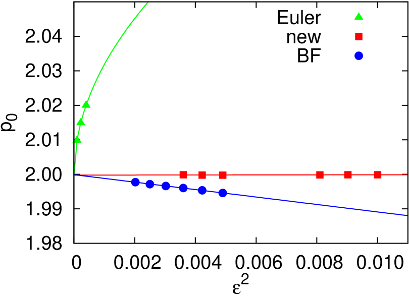
Figure 1: The one-loop plaquette coefficient $p_{0}$ vs. $\epsilon^{2}$ for $N^{4}=10^{4}$: Euler integrator, BF scheme and the new second order integrator.

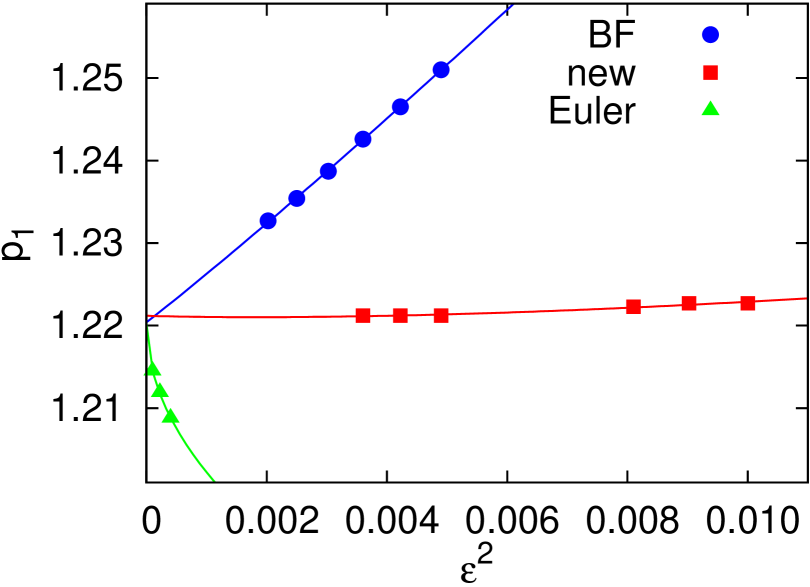
Figure 2: The two-loop plaquette coefficient $p_{1}$ vs. $\epsilon^{2}$ for $N^{4}=10^{4}$: Euler integrator, BF scheme and the new second order integrator.

Figures 1 and 2 illustrate the finite-$\epsilon$ plaquette results for the three integrators: while all sets extrapolate to the same limit within error bars, the ones corresponding to the new second-order scheme are clearly much flatter than the others. In particular, the $\epsilon^{2}$-dependence of the new second-order integrator is greatly reduced compared to the BF scheme of Eqs. (19) and (20). Note that we allowed for cubic terms in the curves drawn for the second order integrators. We will see in Sec. IV below that for the observables of interest in this work extrapolations in $\epsilon^{2}$ are so flat that in most cases a non-trivial slope cannot be resolved within statistical errors.

II.3 Twisted Boundary Conditions

Instead of PBC, one can also impose twisted boundary conditions (TBC) tHooft79 ; Parisi83 ; Luscher86 ; Arroyo88

$$U_{\mu}(n+N_{S}\hat{\nu}) =\Omega_{\nu}U_{\mu}(n)\Omega_{\nu}^{\dagger}\,,$$ (30)

$$U_{\mu}(n-N_{S}\hat{\nu}) =\Omega_{\nu}^{\dagger}U_{\mu}(n)\Omega_{\nu}\,,$$ (31)

where the links that pierce a lattice boundary of a twisted (spatial) direction $\hat{\nu}$ are multiplied by so-called twist matrices $\Omega_{\nu}$ that must satisfy

$$\Omega_{\mu}\Omega_{\nu} =z\,\Omega_{\nu}\Omega_{\mu},$$ (32)

$$\Omega_{\nu}^{3} =\left(-1\right)^{N-1}\mathds{1}\,.$$ (33)

Here $z\in\{\mathds{1},e^{i2\pi/3}\mathds{1},e^{i4\pi/3}\mathds{1}\}$ is an element of the center of $\mathrm{SU}(3)$. The condition Eq. (32) guarantees that the value of the transported link $U_{\mu}\left(n+N_{S}\hat{\mu}+N_{S}\hat{\nu}\right)$ is independent of the order with which two twisted boundaries $\mu,\nu$ are transversed. Gauge transformations $\Lambda(n)$, which rotate the link variables according to

$$U_{\mu}(n)\mapsto\Lambda(n)U_{\mu}(n)\Lambda^{\dagger}(n+\hat{\mu})$$ (34)

must obey the same TBC Eq. (30).

The measure as well as Wilson loops without net winding numbers across boundaries (such as the elementary plaquette within the action) are invariant under the transformation

$$U_{\mu}(n)\to zU_{\mu}(n)\,,\quad\forall\,n\in\{n:n\cdot\hat{\mu}=\mbox{const.}\}\,.$$ (35)

TBC rely on this center symmetry of the $\mathrm{SU}(3)$ gauge action and measure, and can be implemented for the link update either by multiplying the plaquettes in corners of twisted hyper-planes with suitable center elements, or by imposing Eq. (30) with an explicit choice of $\Omega_{\nu}$. We implemented the latter using

$$\Omega_{1}=\left(\begin{array}[]{ccc}0&1&0\\ 0&0&1\\ 1&0&0\end{array}\right)\,,\quad\Omega_{2}=\left(\begin{array}[]{ccc}\zeta^{*}&0&0\\ 0&1&0\\ 0&0&\zeta\end{array}\right)\,,\quad\Omega_{3}=\Omega_{2}\Omega_{1}^{2}=\left(\begin{array}[]{ccc}0&0&\zeta^{*}\\ 1&0&0\\ 0&\zeta&0\end{array}\right)\,,$$ (36)

where $\zeta=e^{2i\pi/3}$, $\zeta^{*}=1/\zeta$. This choice is arbitrary up to global unitary transformations: as long as Eq. (32) is satisfied, the resulting physical amplitudes will not depend on the explicit choice of $\Omega_{\nu}$. As the subscripts indicate, we impose the twist for all spatial directions. Twists in two directions have a non-trivial effect too, while twisting only one direction can be absorbed into a re-definition of the link variables. The effect of twist is twofold: TBC eliminate zero modes which otherwise require an explicit subtraction DR0 . Furthermore, at least at low orders in perturbation theory, TBC reduce finite size effects as the possible gluon momenta are restricted to integer multiples Luscher86 of

$$p_{\nu}=\left\{\begin{array}[]{cl}\frac{2\pi}{3N_{\nu}}\,,&\nu=\mbox{twisted direction}\,,\\ \frac{2\pi}{N_{\nu}}\,,&\nu=\mbox{periodic direction}\,.\end{array}\right.$$ (37)

This means that gluon momenta in twisted spatial directions reach values as low as ${2\pi}/{(3N_{S})}$, compared to ${2\pi}/{N_{S}}$ in periodic directions. So, roughly speaking, the modes in a twisted direction behave as if the corresponding lattice extent was $3N_{S}$ instead of $N_{S}$. We refer to the cases of twists applied to two and three directions as TBCxy and TBCxyz, respectively.

Table 3: Plaquette coefficients. $4^{4}$ PBC: DLPT (first two orders) and NSPT (remaining orders Perlt:privat ). $4^{4}$ TBCxy and TBCxyz: DLPT (first order) and NSPT (remaining orders). $32^{4}$ PBC: DLPT (first two orders) and NSPT ($\mathcal{O}(\beta^{-3})$ DR0 ). Infinite volume: DLPT from Ref. Alles:1998is , using the lattice integrals of Ref. Luscher:1995np . For all NSPT data, the $\epsilon\rightarrow 0$ extrapolation was carried out.

order	$4^{4}$ PBC	$4^{4}$ TBCxy	$4^{4}$ TBCxyz	$32^{4}$ PBC	$\infty^{4}$
$\beta^{-1}$	1.9921875	2	2	1.9999981	2
$\beta^{-2}$	1.2037037	1.2184(5)	1.2200(3)	1.2207904	1.2279575
$\beta^{-3}$	2.887(3)	2.955(2)	2.957(2)	2.957(3)	2.9605(1)
$\beta^{-4}$	-9.05(1)	-9.41(1)	-9.40(1)
$\beta^{-5}$	-32.49(6)	-34.51(9)	-34.34(5)

The effect of TBC is noticeable in particular on small lattice volumes, as Table 3 illustrates for the average plaquette. The two- and three-loop TBCxy and TBCxyz data obtained on $4^{4}$ volumes are close to the infinite volume (as well as to $32^{4}$ PBC) results at two and three loops. This clearly is not the case for $4^{4}$ PBC data. Note that both analytical one-loop TBC coefficients happen to be volume-independent on symmetric lattices, due to cancellations between different plaquette orientations.

The situation is different for the Polyakov loop $L$ defined in Eq. (63) below. First of all, for this observable it matters whether it is obtained in an untwisted or a twisted direction. We calculate $L$ in untwisted directions, for which no modification is necessary with respect to PBC, and extract the static energy $\delta m$ via Eqs. (64)–(65). As it was shown in Ref. Nobes:2001tf for this observable, TBC significantly reduce FSE, resulting in a much flatter extrapolation towards infinite volume. If this flatness at low orders was taken as the only criterion, TBCxy would be the boundary condition of choice. However, it turns out that TBCxy has a draw-back compared to TBCxyz: in non-perturbative simulations only the latter prevents tunneling between different Z(3) phases while TBCxy merely leads to a reduction compared to PBC Trottier:2001vj . As a consequence, small volume TBCxy simulations were found to fluctuate more and to return noisier signals than their TBCxyz counterparts. Regarding the statistical fluctuations we made a similar observation, even though tunneling between Z(3) sectors is not an issue in our NSPT simulations since $U^{(0)}=\mathds{1}$. Fig. 3 shows stochastic time histories obtained on $16^{4}$ volumes at fixed $\epsilon=0.05$ for TBCxy and TBCxyz of the one-loop and 12-loop coefficients of the Polyakov loop. While the trajectories of the one-loop coefficient $L_{0}$ show a similar behavior for TBCxy as for TBCxyz, we observe a peak in the twelve loop $L_{11}$ TBCxy measurement history, which is symptomatic for TBCxy simulations. The enhanced numerical stability and smaller fluctuations, in particular at large orders of expansions, motivated us to choose TBCxyz for this work. A better understanding of the origin of these differences between TBCxy and TBCxyz would be desirable.

 

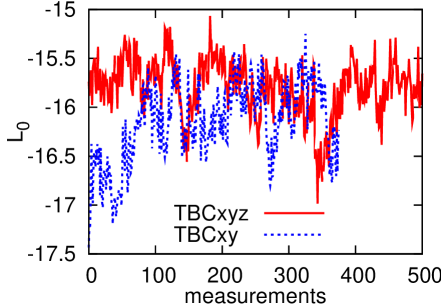
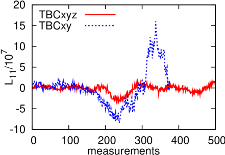
Figure 3: Stochastic time series of one-loop ($L_{0}$, left) and 12-loop ($L_{11}$, right) Polyakov loop coefficients for TBCxyz (blue) and TBCxy (red) on $16^{4}$ lattices for $\epsilon=0.05$.

II.4 Link smearing

The lattice discretization of observables and action is not unique. For instance one can construct Wilson loops and Polyakov loops, replacing the link variables $U_{\mu}(n)$ by fat or “smeared” links. In the context of a lattice determination of static potentials and of static-light meson masses this was for instance done in Ref. Bali:2005fu , to reduce the self-energy, enabling an improved signal to noise ratio at large Euclidean times. As long as the smearing is an ultra-local procedure, defined on the scale of a few lattice spacings, making this replacement in a Polyakov loop corresponds to a different choice of discretization of the static action. Smearing is sometimes also used within the definition of fermionic actions, see, e.g., Refs. Blum:1996uf ; Zanotti:2001yb ; Capitani:2006ni .

Several smearing methods are available, one of which is known as analytic or “stout” smearing Morningstar:2003gk . Stout links are automatically elements of the $\mathrm{SU}(3)$ group, without a numerically delicate projection into the group. Therefore, implementing stout smearing within a perturbative expansion is straightforward. Stout smeared links are obtained by the replacement

$$U_{\mu}(n)\mapsto U_{\mu}^{\mathrm{stout}}(n)=\exp(iQ_{\mu}(n))U_{\mu}(n),$$ (38)

where $Q_{\mu}(n)$ is Hermitian and traceless and hence in the algebra by design:

$$Q_{\mu}(n) =\frac{i}{2}\left[R_{\mu}^{\dagger}(n)-R_{\mu}(n)-\frac{1}{3}\mathrm{tr}\left(R_{\mu}^{\dagger}(n)-R_{\mu}(n)\right)\mathds{1}\right]\,\ ,$$ (39)

$$R_{\mu}(n) =C_{\mu}(n)U^{\dagger}_{\mu}(n)\,\ ,$$ (40)

$$C_{\mu}(n) =\sum_{\nu\neq\mu}\rho_{\mu\nu}(U_{\nu}(n)U_{\mu}(n+\hat{\nu})U^{\dagger}_{\nu}(n+\hat{\mu})+U^{\dagger}_{\nu}(n-\hat{\nu})U_{\mu}(n-\hat{\nu})U_{\nu}(n-\hat{\nu}+\hat{\mu}))\,.$$ (41)

Note that within the sum of staples $C_{\mu}(n)$, surrounding the link $U_{\mu}(n)$, the sum convention is not implied and $\rho_{\mu\nu}$ are weights that can be set at will. In our case, we choose $\rho_{i\nu}=0$ and $\rho_{4i}\equiv\rho=1/6$ otherwise. The value of the weight was chosen to minimize the one-loop static self-energy after one smearing iteration. We remark that this is not necessarily the best possible choice, e.g., in a non-perturbative setting. We apply only one smearing step to keep the static action local.

III Self-energy of a static source

In this section we introduce our conventions, relate self-energies of static sources to heavy quark and heavy gluino pole masses, and discuss the expected renormalon structure.

The triplet and octet self-energies are defined as the lowest energy eigenvalues of the effective Hamilton operator in temporal gauge of the sector of Hilbert space of gauge triplet and octet states with respect to gauge transformations, applied to a fixed position. It is impossible to obtain the continuum limit for these self-energies (irrespectively of the representation), as these will diverge linearly with the ultraviolet cut-off. Therefore, the value of the static self-energy depends on the chosen regulator. Yet, any hard-cut-off regularization scheme is suitable for the following discussion. In this article we use lattice regularization and write the self-energies in the fundamental and adjoint representation in the following way:

$$\delta m=\frac{1}{a}\sum_{n=0}^{\infty}c^{(3,\rho)}_{n}\alpha^{n+1}(1/a)\,\mathrm{(fundamental)},\qquad\delta m_{\tilde{g}}=\frac{1}{a}\sum_{n=0}^{\infty}c^{(8,\rho)}_{n}\alpha^{n+1}(1/a)\,\mathrm{(adjoint)}\,,$$ (42)

where $a^{-1}$, the inverse lattice spacing, provides the ultraviolet cut-off. The coefficients $c_{n}$ depend on the details of the regularization, i.e., on the action used and the specific definition of the static propagator. We only consider the Wilson action Wilson:1974sk but we explore two different definitions of the static propagator, with smeared ($\rho=1/6$) and with the original ($\rho=0$) temporal links. We label this dependence with a generic $\rho\in\{0,1/6\}$, see Sec. II.4 above.

One may suspect that the dependence on the regulator might turn this object uninteresting from the theoretical point of view. This is actually not the case since, for large $n$, $c_{n}$ becomes regulator independent, universal and equal to $r_{n}/\nu$, the $n+1$ order coefficient of the perturbative expansion of the pole mass

$$m_{\mathrm{OS}}=m_{\overline{\mathrm{MS}}}(\nu)+\sum_{n=0}^{\infty}r_{n}\alpha_{\mathrm{s}}^{n+1}(\nu)\,\ ,$$ (43)

up to $\mathcal{O}[\exp(-1/n)]$-terms (due to subleading renormalons). On an intuitive level this is clear, as the static energy and pole mass share exactly the same infrared behavior (up to $\mathcal{O}(1/m)$ corrections), which should cancel in the difference.

The asymptotic behavior of $r_{n}$ can be determined assuming that the perturbative series is asymptotic and the validity of the OPE. The running of $\alpha(\nu)$ is governed by the $\beta$-function

$$\beta(\alpha)=\frac{d\alpha}{d\ln\nu}=-2\alpha\left[\beta_{0}\frac{\alpha}{4\pi}+\beta_{1}\left(\frac{\alpha}{4\pi}\right)^{2}+\beta_{2}\left(\frac{\alpha}{4\pi}\right)^{3}+\ldots\right]\ ,$$ (44)

where in our normalization

$$\beta_{0}=11\,,\quad\beta_{1}=102\,,\quad\beta_{2}^{\overline{\mathrm{MS}}}=\frac{2857}{2}\,,\quad\beta_{2}^{\mathrm{latt}}=-6299.8999(6)\,.$$ (45)

From $\beta_{2}$ onwards the coefficients depend on the scheme. While $\beta_{3}^{\overline{\mathrm{MS}}}$ is known vanRitbergen:1997va , in the lattice scheme only $\beta_{2}^{\mathrm{latt}}$ has been computed Luscher:1995np ; Christou:1998ws ; Bode:2001uz . For convenience we define the constants

$$b =\frac{\beta_{1}}{2\beta_{0}^{2}}\,,$$ (46)

$$s_{1} =\frac{\beta_{1}^{2}-\beta_{0}\beta_{2}}{4b\beta_{0}^{4}}\,,$$ (47)

$$s_{2} =\frac{\beta_{1}^{4}+4\beta_{0}^{3}\beta_{1}\beta_{2}-2\beta_{0}\beta_{1}^{2}\beta_{2}+\beta_{0}^{2}(-2\beta_{1}^{3}+\beta_{2}^{2})-2\beta_{0}^{4}\beta_{3}}{32b(b-1)\beta_{0}^{8}}\,,$$ (48)

where only $b$ is scheme-independent. In a given scheme, the $\Lambda$ parameter is defined as

$$\Lambda =\lim_{\nu\rightarrow\infty}\nu e^{-\left[b\ln\left(\frac{\beta_{0}}{4\pi}\right)+\int^{\alpha(\nu)}\!\frac{d\alpha^{\prime}}{\beta(\alpha^{\prime})}\right]}$$ (49)

$$=\nu e^{-\frac{2\pi}{\beta_{0}\alpha(\nu)}}\left(\frac{\beta_{0}\alpha(\nu)}{4\pi}\right)^{-b}\left[1+s_{1}b\frac{\beta_{0}\alpha(\nu)}{2\pi}+s_{2}b(b-1)\left(\frac{\beta_{0}\alpha(\nu)}{2\pi}\right)^{2}+\cdots\right]\,,$$

and we use $\Lambda_{\mathrm{QCD}}\sim\Lambda_{\overline{\mathrm{MS}}}$ synonymously with the size of a typical non-perturbative binding energy.

A simple scheme- and scale-independent observable is the $B$ meson mass. In the heavy quark limit this can be decomposed into the $b$-quark pole mass $m_{\mathrm{OS}}$ and the remaining energy from the light quark and gluon dynamics $\Lambda_{B}=c_{B}\Lambda_{\mathrm{QCD}}$:

$$m_{B}=m_{\mathrm{OS}}+\Lambda_{B}+\mathcal{O}\left(\frac{1}{m_{\mathrm{OS}}}\right)\,.$$ (50)

This relates to the fundamental representation. For the adjoint representation we can think of a heavy gluino attached to gluons:

$$m_{\tilde{G}}=m_{{\tilde{g}},\mathrm{OS}}+\Lambda_{H}+\mathcal{O}\left(\frac{1}{m_{{\tilde{g}},\mathrm{OS}}}\right)\,,$$ (51)

where $\Lambda_{H}$ denotes the dynamical contribution of the gluons (and sea quarks) to the gluinonium mass. For both representations the uncertainty of the perturbative series of the pole mass will be of $\mathcal{O}(\Lambda_{\mathrm{QCD}})$, the next term in the OPE, since only the sum of the pole mass and the binding energy has a physical meaning. This ambiguity results in the successive contributions $r_{n}\alpha^{n+1}$ to decrease for small orders $n$ down to a minimum at $n_{0}\sim 1/(|a_{d}|\alpha)$, where $a_{d}=\beta_{0}/(2\pi d)$ with $d=1$. After this order the series starts to diverge, so one neglects the higher order contributions and estimates the error by the size of this minimum term, $r_{n_{0}}\alpha^{n_{0}+1}\sim\exp[-1/(a_{d}\alpha)]\sim\Lambda_{\mathrm{QCD}}/m$. If the perturbative expansion has an ambiguity of order $\Lambda_{\mathrm{QCD}}^{n}$ then $d=n$. To quantify this behavior it is convenient to consider the Borel transform of the above perturbative series

$$m_{\mathrm{OS}}=m_{\overline{\mathrm{MS}}}+\int\limits_{0}^{\infty}\!dt\,e^{-t/\alpha_{\mathrm{s}}}\,B[m_{\mathrm{OS}}](t)\,,\quad B[m_{\mathrm{OS}}](t)\equiv\sum_{n=0}^{\infty}r_{n}\frac{t^{n}}{n!}\,.$$ (52)

The behavior of the expansion Eq. (43) at large orders is dictated by the closest singularity to the origin of its Borel transform, which, for the pole mass, is located at $t=2\pi/\beta_{0}$, i.e., at $u=1/2$, defining $u=\frac{\beta_{0}t}{4\pi}$. More precisely, the behavior of the Borel transform near the closest singularity at the origin reads

$$B[m_{\mathrm{OS}}](t(u))=N_{m}\nu\frac{1}{(1-2u)^{1+b}}\left(1+s_{1}(1-2u)+s_{2}(1-2u)^{2}+\cdots\right)+(\mathrm{analytic\;term}),$$ (53)

where by analytic term we mean contributions that are expected to be analytic up to the next renormalon ($u=1$). This dictates the behavior of the perturbative expansion at large orders to be

$$r_{n}\stackrel{{\scriptstyle n\rightarrow\infty}}{{=}}N_{m}\,\nu\,\left(\frac{\beta_{0}}{2\pi}\right)^{n}\,\frac{\Gamma(n+1+b)}{\Gamma(1+b)}\left(1+\frac{b}{(n+b)}s_{1}+\frac{b(b-1)}{(n+b)(n+b-1)}s_{2}+\cdots\right).$$ (54)

This expression can be obtained from the procedure employed in Ref. Beneke:1994rs . The $s_{1}$-term was computed in Ref. Beneke:1994rs , and the $s_{2}$-term in Refs. Pineda:2001zq ; Beneke:1998ui .

As we mentioned, the large-$n$ behavior of $c^{(3,\rho)}_{n}$ is the same as that of $r_{n}$ up to $\mathcal{O}(e^{-1/n})$-terms (due to subleading renormalons). Therefore, using the same scheme for the expansion parameter $\alpha$, we obtain

$$c^{(3,\rho)}_{n}\stackrel{{\scriptstyle n\rightarrow\infty}}{{=}}N_{m}\,\left(\frac{\beta_{0}}{2\pi}\right)^{n}\,\frac{\Gamma(n+1+b)}{\Gamma(1+b)}\left(1+\frac{b}{(n+b)}s_{1}+\frac{b(b-1)}{(n+b)(n+b-1)}s_{2}+\cdots\right).$$ (55)

Note that all the dependence on the regularization details (and in particular on $\rho$) vanishes. The normalization constant $N_{m}$ also determines the strength of the renormalon of the singlet static potential, through the relation

$$2N_{m}+N_{V_{s}}=0\,,$$ (56)

since these contributions cancel from the energy $E(r)=2m+V_{s}(r)$ Pineda:1998id ; Hoang:1998nz ; Beneke:1998rk .

For adjoint sources we have

$$c^{(8,\rho)}_{n}\stackrel{{\scriptstyle n\rightarrow\infty}}{{=}}N_{m_{\tilde{g}}}\,\left(\frac{\beta_{0}}{2\pi}\right)^{n}\,\frac{\Gamma(n+1+b)}{\Gamma(1+b)}\left(1+\frac{b}{(n+b)}s_{1}+\frac{b(b-1)}{(n+b)(n+b-1)}s_{2}+\cdots\right)\,.$$ (57)

Again, the dependence on the regularization details (e.g. on $\rho$) vanishes, however, the octet normalization is different: $N_{m_{\tilde{g}}}\neq N_{m}$. Eq. (57) corresponds to the renormalon of gluelump masses (actually $N_{m_{\tilde{g}}}=-N_{\Lambda}$, where $N_{\Lambda}$ is the strength of the gluelump renormalon associated to $\Lambda_{H}$) and can be related to the pole mass and adjoint static potential renormalons through the relation

$$2N_{m}+N_{V_{0}}+N_{\Lambda}=0\,,$$ (58)

since the energy $E(r)=2m+V_{o}(r)+\Lambda_{H}$ is renormalon free Bali:2003jq .

To eliminate the unknown normalization constants, we may consider ratios. In a strict $1/n$ expansion we have

$$\frac{c^{(3,\rho)}_{n}}{c^{(3,\rho)}_{n-1}}\frac{1}{n}=\frac{c^{(8,\rho)}_{n}}{c^{(8,\rho)}_{n-1}}\frac{1}{n}$$ (59)

$$\quad=\frac{\beta_{0}}{2\pi}\left\{1+\frac{b}{n}-\frac{bs_{1}}{n^{2}}+\frac{1}{n^{3}}\left[b^{2}s_{1}^{2}+b(b-1)(s_{1}-2s_{2})\right]+\mathcal{O}\left(\frac{1}{n^{4}}\right)\right\}\,\ .$$

This expression holds in any representation. It is also independent of the renormalization scheme used for $\alpha$. Keep in mind though that the explicit expression does depend on the scheme, starting from $\beta_{2}$. Here we will mainly use $\alpha_{\mathrm{latt}}$, where $s_{2}$ is unknown and $\beta_{2}=\beta_{2}^{\mathrm{latt}}$, but we will also consider the behavior of the perturbative series in the $\overline{\mathrm{MS}}$ scheme.

Assuming that the coefficients are dominated by the renormalon behavior, we can determine the order $n_{0}+1$ that corresponds to the minimal term within the pole mass perturbative series. Minimizing $r_{n}\alpha^{n+1}$ results in

$$(n_{0}+b)\frac{\beta_{0}\alpha}{2\pi}=\exp\left\{-\frac{1}{2(n_{0}+b)}+\mathcal{O}\left[\frac{1}{(n_{0}+b)^{2}}\right]\right\}\,.$$ (60)

This yields the minimal term

$$r_{n_{0}}\alpha^{n_{0}+1}(\nu)=\frac{2^{1-b}\pi}{\Gamma{(1+b)}}\sqrt{\frac{\alpha(\nu)}{\beta_{0}}}N_{m}\Lambda\left[1+\mathcal{O}(\alpha)\right]\,.$$ (61)

While it is evident to most readers, we wish to emphasize that the perturbative series that defines the pole mass cannot be resummed (not even in a Borel way). Therefore, it does not exist in a mathematical sense and no rigorous numerical value or error can be assigned to this object. The most one could do is to define a pole mass to a given (finite) order $N+1$, $m_{\mathrm{OS}}^{(N)}\equiv\sum_{n=0}^{N}r_{n}\alpha^{n+1}$, which will then depend on $N$. By taking $N\sim n_{0}$ we minimize this dependence. One can then estimate the uncertainty of the sum to be (see, for instance, the discussion in Ref. Sumino:2005cq )

$$\sqrt{n_{0}}\,|r_{n_{0}}|\alpha^{n_{0}+1}(\nu)=\frac{2^{3/2-b}\pi^{3/2}}{\Gamma{(1+b)}}\frac{|N_{m}|\Lambda}{\beta_{0}}\,.$$ (62)

Note that this object is scheme and scale independent (to the $1/n$-precision that we employed in the derivation) because, even though the normalizations $N_{m}$ and $N_{m_{\tilde{g}}}$ depend on the scheme, the products $N_{m}\Lambda$ and $N_{m_{\tilde{g}}}\Lambda$ are scheme-independent.

IV The Polyakov loop

We obtain the coefficients $c_{n}$ from the temporal Polyakov loop on hyper-cubic lattices. We investigate volumes of $N_{T}$ lattice points in the time direction and spatial extents of $N_{S}$ points. We choose PBC in time and TBC in all spatial directions (TBCxyz, see Sec. II.3), eliminating zero modes and improving the numerical stability. For test purposes, we have performed additional simulations with PBC in all spatial directions to $\mathcal{O}(\alpha^{32})$ for a $4^{3}\times 8$ volume and to lower orders for the specific volumes listed in the second row of Table 4.

Table 4: The $N_{S}(N_{T})$ values of the PBC and TBC runs. The different geometries are grouped in terms of the orders of the respective expansions $\mathcal{O}(\alpha^{{n_{\mathrm{max}}}+1})$.

	$\mathcal{O}(\alpha^{3})$	$\mathcal{O}(\alpha^{4})$	$\mathcal{O}(\alpha^{12})$	$\mathcal{O}(\alpha^{20})$
PBC		4 (4)		8 (8,10,12,14)
TBC	5 (5,6,7,8,10)	4 (5,6,7,8,10,12,16,20,24)	6 (6,8,10,12,16)	7 (7,8)
			8 (12,16)	8 (8,10), 9 (12)
			10 (8,12,16,20)	10 (10), 11 (16)
		12 (16,20)	16 (12,16,20)	12 (12), 14(14)

The Polyakov loop is defined as

$$L^{(R)}(N_{S},N_{T})=\frac{1}{N_{S}^{3}}\sum_{\mathbf{n}}\frac{1}{d_{R}}\mathrm{tr}\left[\prod_{n_{4}=0}^{N_{T}-1}U^{R}_{4}(n)\right]\,,$$ (63)

where $U^{R}_{\mu}(n)\approx e^{iA^{R}_{\mu}[(n+1/2)a]}\in\mathrm{SU(3)}$ denotes a gauge link in representation $R$, connecting the sites $n$ and $n+\hat{\mu}$, $n_{i}\in\{0,\ldots,N_{S}-1\}$, $n_{4}\in\{0,\ldots,N_{T}-1\}$. We implement triplet and octet representations $R$ of dimensions $d_{R}=3$ and 8. The link $U_{4}(n)$ appears within the covariant derivative of the static action $\bar{\psi}D_{4}\psi$, acting in the following way on a scalar lattice field $f(n)$: $D_{4}f(n)=[U_{4}(n)f(n+\hat{4})-U_{4}^{\dagger}(n-\hat{4})f(n-\hat{4})]/(2a)$. This discretization is not unique and we may substitute $U_{4}$ by another gauge covariant connection. We use singly stout-smeared Morningstar:2003gk covariant transporters (smearing parameter $\rho=1/6$, see Sec. II.4) instead of $U_{4}(n)$ as a second, alternative choice, to verify the universality of our findings.

We perturbatively expand the logarithm of the Polyakov loop

$$P^{(R,\rho)}(N_{S},N_{T})=-\frac{\ln\langle L^{(R,\rho)}(N_{S},N_{T})\rangle}{aN_{T}}=\sum_{n=0}^{\infty}c^{(R,\rho)}_{n}(N_{S},N_{T})\alpha^{n+1}\,,$$ (64)

in order to obtain the static triplet and octet self-energies in the infinite volume limit:

$$\delta m=\lim_{N_{S},N_{T}\rightarrow\infty}P^{(3,\rho)}(N_{S},N_{T})\,,\qquad\delta m_{\tilde{g}}=\lim_{N_{S},N_{T}\rightarrow\infty}P^{(8,\rho)}(N_{S},N_{T})\ ,$$ (65)

where (see Eq. (42))

$$c^{(R,\rho)}_{n}=\lim_{N_{S},N_{T}\rightarrow\infty}c_{n}^{(R,\rho)}(N_{S},N_{T})\,.$$ (66)

The primary objects that we compute are the coefficients $c_{n}(N_{S},N_{T})$. The sets of $c_{n}(N_{S},N_{T})$ obtained on different geometries are statistically independent of one another. However, for a given volume, different orders $n$ will be correlated. In computations of ratios $c_{n}(N_{S},N_{T})/c_{n-1}(N_{S},N_{T})$, as well as in fits, we take these correlations into account. NSPT enables us to calculate the coefficients directly, i.e., that neither the lattice spacing nor the strong coupling parameter $\alpha$ enter the simulation. We have realized a large variety of TBC geometries, listed in Table 4, in addition to the PBC test runs. Each coefficient $c_{n}$ depends on $N_{S}$ and $N_{T}$ but also on the time step $\epsilon$ of the Langevin evolution (see below). In this paper we employ the variant of the Langevin algorithm introduced in Ref. Torrero:08 and explained in Sec. II.2, which only quadratically depends on $\epsilon$. The time series were analyzed following Ref. Wolff:2003sm , allowing us to process either single runs or to evaluate sets of “farmed out” Monte Carlo branches. Special care was taken to ensure that every individual history for each order was sufficiently long relative to the respective autocorrelation time to guarantee a safe error analysis. Branches that failed this test were removed from the data analysis.

Very high statistics runs were performed up to $\mathcal{O}(\alpha^{3})$ and $\mathcal{O}(\alpha^{4})$, to check if the coefficients of logs extracted from the data are in agreement with our theoretical expectations, to detect signs of ultrasoft $\ln(N_{T}/N_{S})$-terms (see Secs. V and VI below), and to compare with results from diagrammatic perturbation theory.

The bulk of data are obtained up to $\mathcal{O}(\alpha^{12})$ and $\mathcal{O}(\alpha^{20})$. We have kept the Langevin time between two successive measurements fixed, adjusting $n_{\mathrm{upd}}\approx 56/\epsilon$ where $n_{\mathrm{upd}}$ is the number of updates performed in between two measurements. For the $\alpha^{12}$ and $\alpha^{20}$ runs between 35000 and 80000 measurements were taken, corresponding (for $\epsilon=0.050$) to $4\times 10^{7}$ – $9\times 10^{7}$ updates. The integrated autocorrelation times increase with the order of the expansion and with the lattice volume. For instance, the integrated autocorrelation time of $c_{0}$ varied from 2.4 ($6^{4}$) to 15 ($16^{4}$), while that of $c_{11}$ from $9$ to $30$, in units of $n_{\mathrm{upd}}$. For our highest order coefficient $c_{19}$ we found the values $\tau_{\mathrm{int}}\approx 18$ and 29 for $11^{3}\times 16$ and $12^{4}$ lattices respectively. Since the $\epsilon=0.050$ measurements are separated by 1120 Langevin updates, our largest $\tau_{\mathrm{int}}=30$ value corresponds to more than 33000 such updates, still leaving us with a few hundred effectively statistically independent measurements.

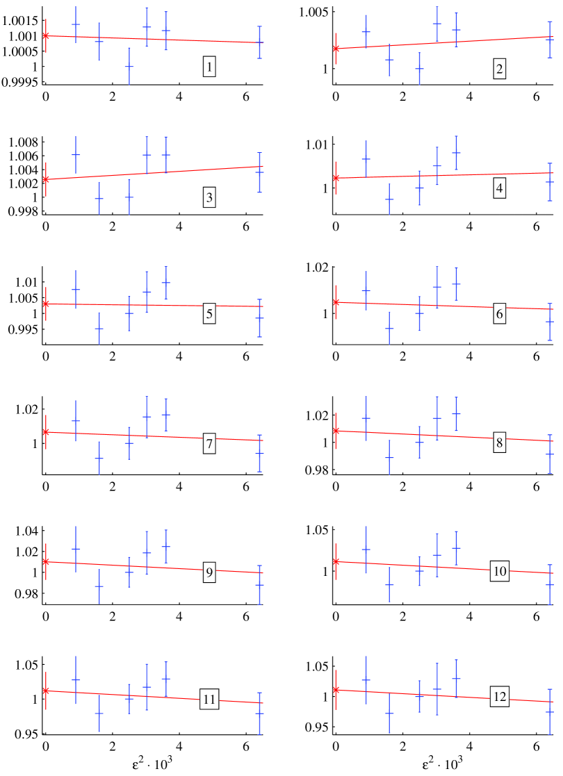
Figure 4: Time step extrapolations of ratios $c^{(3,0)}_{n}(16,16;\epsilon)/c^{(3,0)}_{n}(16,16;0.05)$ (blue symbols) for $\epsilon\in\{0.03,0.04,0.05,0.055,0.06,0.08\}$ at different orders $n+1=1,\ldots,12$. The left-most red symbols are the extrapolated values.

Quadratic extrapolations in the Langevin time step to $\epsilon=0$ on a $16^{4}$ lattice (based on 6 $\epsilon$-values) and on a $6^{4}$ lattice (4 $\epsilon$-values) were performed up to $\mathcal{O}(\alpha^{12})$. The $16^{4}$ extrapolation, normalized to the value obtained at $\epsilon=0.05$ ($10^{3}\epsilon^{2}=2.5$) is shown for the unsmeared triplet coefficients $c_{n}^{(3,0)}(16,16)$ in Fig. 4, up to $n=11$. A similar picture arises for the $6^{4}$ volume: within two standard deviations the extrapolated values are all found to agree with the results obtained at $\epsilon=0.05$. We remark that for both volumes the fit functions are quite flat, with very small slopes in $\epsilon^{2}$. The same was observed for the smeared and the octet coefficients. Based on this experience, the remaining volumes are only simulated for $\epsilon=0.05$. However, the time step scaling was only tested within certain errors that are similar in size as (and in some cases larger than) the statistical errors obtained for the various geometries. We obtain a relative systematic error for each order by adding the statistical error of the extrapolation and the difference of the extrapolated value from unity in quadrature. For the other geometries this (multiplied by the $\epsilon=0.05$ coefficient) is then added in quadrature to the respective statistical error. For orders larger than $n+1=12$, we linearly extrapolate in $n$ the systematics found for orders $n+1\leq 12$, to obtain an estimate. This procedure is performed not only for the coefficients themselves but also for ratios of coefficients. While the systematic time step error is assumed to be uncorrelated, we keep track of the correlation between the statistical part of the errors for different orders $n$, obtained on the same volume.

V Finite size effects for $N_{T}\rightarrow\infty$

The finite size effects of $P(N_{S},N_{T})$ [Eq. (64)] are well suited to a theoretical analysis in the limit $N_{T}\rightarrow\infty$ (actually $N_{T}\geq N_{S}$ for most of the geometries that we simulate). In this limit the self-energy of a static source in a finite spatial volume is obtained:

$$\delta m(N_{S})=\lim_{N_{T}\rightarrow\infty}P(N_{S},N_{T})\qquad\mathrm{and}\qquad c_{n}(N_{S})=\lim_{N_{T}\rightarrow\infty}c_{n}(N_{S},N_{T})\,.$$ (67)

For large $N_{S}$, we write

$$c_{n}(N_{S})=c_{n}-\frac{f_{n}(N_{S})}{N_{S}}+\mathcal{O}{\left(\frac{1}{N_{S}^{2}}\right)}\ .$$ (68)

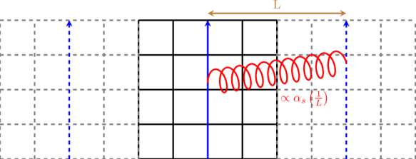
Figure 5: Self-interactions with replicas producing $1/L=1/(aN_{S})$ Coulomb terms.

The $\mathcal{O}(1/N_{S})$ correction originates from interactions with mirror images at distances $aN_{S}$, $\sqrt{2}aN_{S}$, $\sqrt{3}aN_{S}$, $2aN_{S}$, $\ldots$, see also Ref. Trottier:2001vj . This effectively produces a static potential between charges separated at distances $aN_{S}$, but without self-energies (the self-energies are included in $\delta m$). As illustrated in Fig. 5, the scale of such interactions is of order $aN_{S}$ and one may write

$$\delta m(N_{S})=\delta m-\frac{1}{aN_{S}}\sum_{n=0}^{\infty}f_{n}\alpha^{n+1}\!\!\left(\left(aN_{S}\right)^{-1}\right)+\mathcal{O}{\left(\frac{1}{N_{S}^{2}}\right)}\,.$$ (69)

Therefore, the coefficient $f_{n}(N_{S})$ is a polynomial of $\ln(N_{S})$:

$$f_{n}(N_{S})=\sum_{i=0}^{n}f_{n}^{(i)}\ln^{i}(N_{S})\,,$$ (70)

where $f_{n}^{(0)}=f_{n}$ and the coefficients $f_{n}^{(i)}$ for $i>0$ are entirely determined by $f_{m}$ with $m<n$ and $\beta_{j}$ (see Eq. (44)), with $j\leq n-1$. For instance,

$$f_{1}(N_{S}) =f_{1}+f_{0}\frac{\beta_{0}}{2\pi}\ln(N_{S})\,,$$ (71)

$$f_{2}(N_{S}) =f_{2}+\left[2f_{1}\frac{\beta_{0}}{2\pi}+f_{0}\frac{\beta_{1}}{8\pi^{2}}\right]\ln(N_{S})+f_{0}\left(\frac{\beta_{0}}{2\pi}\right)^{\!\!2}\!\ln^{2}(N_{S})\,,$$ (72)

and so on.

Starting at $\mathcal{O}(\alpha^{4})$, one may expect additional $\mathcal{O}(1/N_{S})$ finite size terms. These would arise from infrared singularities of certain types of diagrams. The source of these infrared singularities is similar to the one that results in infrared divergences of the static potential Appelquist:1977es starting at $\mathcal{O}(\alpha^{4})$. In that case these are due to the static triplet and antitriplet sources, which can arrange themselves into a singlet or into an octet representation at short distances in the pNRQCD Brambilla:1999qa multipole expansion, giving rise to terms like $\alpha_{\mathrm{s}}^{4}\ln(aN_{S}\mu_{\mathrm{IR}})/(aN_{S})$. In our case, pairs of triplet static sources can be arranged into antitriplet and sextet representations with their mixing mediated through gluons. At higher orders different representations can arise, as several mirror images will interact. Nevertheless, in the limit $N_{T}\rightarrow\infty$ in a finite spatial volume, we do not expect these ultrasoft logarithms to show up. The reason is that $aN_{S}$, besides being the typical momentum transfer between the mirror images, is also the infrared cut-off of the gluon momenta so that only logarithmic terms $\sim\ln(N_{S}/N_{S})$ can appear. Indeed we do not detect any indication of these logs in our numerical data.

Eq. (69) can be interpreted in terms of renormalons. The fact that we can link the $\mathcal{O}(1/N_{S})$-term to a static potential leads to the expectation that the high order behaviors of $f_{n}$ and $c_{n}$ are dominated by one and the very same renormalon. This can, e.g., be illustrated considering the leading dressed gluon propagator $D(k)\propto 1/k^{2}$, where $k_{4}=0$. With the (formal) ultraviolet cut-off $1/a$ and an infrared cut-off $1/(aN_{S})$ this can be written as (ignoring lattice corrections),

$$P \propto\int_{1/(aN_{S})}^{1/a}\!\!\!\!dk\,k^{2}D(k)\sim\frac{1}{a}\sum_{n}c_{n}\alpha^{n+1}\!\left(a^{-1}\right)-\frac{1}{aN_{S}}\sum_{n}c_{n}\alpha^{n+1}\!\left((aN_{S})^{-1}\right)\,,$$ (73)

after perturbatively expanding $D(k)$. When re-expressing $\alpha((aN_{S})^{-1})$ in terms of $\alpha(a^{-1})$ we may consider two situations:
(a) $N_{S}>e^{n}$. In this limit the last term of Eq. (73) is exponentially suppressed in $n$ and the renormalon can directly be obtained from a large order expansion of $aP$ in powers of $\alpha$.
(b) $N_{S}<e^{n}$. The last term of Eq. (73) is important and the renormalon cancels order-by-order in $n$. It is easy to visualize the importance of this term in the large-$\beta_{0}$ limit (see the discussion in Ref. Pineda:2005kv ). In this limit one obtains

$$\alpha\left(\frac{1}{aN_{S}}\right) =\sum_{n\geq 0}\frac{\ln^{n}(N_{S})}{n!}\left(\frac{d\alpha}{d\ln a}\right)^{n}$$

$$\stackrel{{\scriptstyle\mathrm{large}\,\beta_{0}}}{{\quad=\quad}}\sum_{n\geq 0}\left(\frac{\beta_{0}}{2\pi}\right)^{n}\ln^{n}(N_{S})\,\alpha^{n+1}\left(a^{-1}\right)\ ,$$ (74)

and therefore the large-$n$ behaviors of $c_{n}$ and $f^{(i)}_{n}(N_{S})$ read

$$c_{n}\simeq N_{m}\left(\frac{\beta_{0}}{2\pi}\right)^{n}n!\,,\qquad f^{(i)}_{n}(N_{S})\simeq N_{m}\left(\frac{\beta_{0}}{2\pi}\right)^{n}\frac{n!}{i!}\,.$$ (75)

This results in the logarithms of Eq. (70) to exponentiate and to cancel the $1/N_{S}$ suppression. Therefore, at large $n$, the $f_{n}/N_{S}$ terms become numerically as important as the $c_{n}$-terms so that

$$c_{n}-\frac{f_{n}(N_{S})}{N_{S}} \simeq N_{m}\left(\frac{\beta_{0}}{2\pi}\right)^{n}n!\left(1-\frac{e^{\ln N_{S}}}{N_{S}}+\frac{1}{N_{S}}\sum_{i=n+1}^{\infty}\frac{1}{i!}\ln^{i}N_{S}\right)$$

$$=\frac{1}{N_{S}}N_{m}\left(\frac{\beta_{0}}{2\pi}\right)^{n}n!\sum_{i=n+1}^{\infty}\frac{1}{i!}\ln^{i}(N_{S})\,.$$ (76)

Note that the renormalon ($n!$ behavior) actually cancels in the difference and that the infinite sum above is a convergent series ($N_{S}$ minus a finite sum).

In present-day numerical simulations, including ours, $N_{S}<e^{n}$, and the term $f_{n}(N_{S})/N_{S}$ needs to be taken into account, in combination with $c_{n}$. A similar phenomenon was numerically observed for the static singlet energy $E(r)=2m+V(r)$ Pineda:2002se ; Bali:2003jq . This teaches us that to correctly identify the renormalon structure of $\delta m$, it is compulsory to incorporate the $1/N_{S}$ corrections. So far, in studies of high order perturbative expansions of the plaquette the corresponding finite size terms have been neglected. As we will see, our fits indeed yield $f_{n}\simeq c_{n}$ for large $n$, in clear support of the renormalon dominance picture.

In the $N_{T}\rightarrow\infty$ limit, and up to $\mathcal{O}(1/N_{S}^{2})$ effects, the fit function for $c_{n}(N_{S})$ depends on $c_{n}$, $f_{n}$ and the $\beta$-function coefficients $\beta_{i}$ with $i<n$. In the lattice scheme only $\beta_{0}$, $\beta_{1}$ and $\beta_{2}$ are known. The effects of higher $\beta_{j}$ start at $\mathcal{O}(\alpha^{5})$. One may try to fit these, together with the $c_{n}$ and $f_{n}$ but their contribution cannot be resolved by the present precision of the data. This produces some uncertainty in our parametrization that we will add to the error. The reason we can neglect higher $\beta_{j}$ in a controlled way is because the associated uncertainty quickly becomes negligible at high orders, once the behavior of the coefficients $f_{n}$ starts to be governed by the $d=1$ renormalon. This statement can be quantified, since we know the large-$n$ behavior of the $f^{(j)}_{n}$. Let us first consider the large-$\beta_{0}$ limit. Assuming renormalon dominance for the coefficients $f_{n}$, we would have (see Eqs. (75) and (V))

$$f_{n}(N_{S})=N_{m}\left(\frac{\beta_{0}}{2\pi}\right)^{n}n!\sum_{i=0}^{n}\frac{1}{i!}\ln^{i}(N_{S})\,.$$ (77)

Note that terms containing higher powers of $\ln(N_{S})$ (with $i\lesssim n$) are suppressed by factors $\sim 1/n!$ and can be neglected at large $n$. Therefore, for large $n$, the $n!$ factorial overcomes the large logs. This suppression also holds beyond the large-$\beta_{0}$ limit. However, we may worry about terms with small powers of $\ln(N_{S})$ ($i\sim 1$ in Eq. (77)). In this case there is no factorial suppression, but the inclusion of $\beta_{1}$ and $\beta_{2}$ can still be done in a controlled way. Including the running associated to $\beta_{1}$ produces $1/n$ suppressed corrections to Eq. (75) while $\beta_{2}$ results in $1/n^{2}$ suppression and so on. For instance in the case of $f_{n}^{(1)}$ we have

$$f_{n}^{(1)}=N_{m}\,\nu\,\left(\frac{\beta_{0}}{2\pi}\right)^{n}\,\frac{\Gamma(n+1+b)}{\Gamma(1+b)}\left[1+\frac{b}{(n+b)}\frac{n-1}{(n-1+b)}+\mathcal{O}\left(1/n^{2}\right)\right]\,.$$ (78)

To check this assumption and to justify the truncation at $\beta_{2}$ we have performed separate fits including $\beta_{j}$ for $j\leq 0,1$ and 2 (see Sec. VII).

Finally note that the validity of the above discussion is unaffected by any renormalon (or other singularity) related to the $\beta$-function coefficients, as this would correspond to a higher dimension, i.e., $u>1/2$ (if it existed at all).

VI $1/N_{T}$- and subleading $1/N_{S}$-corrections

While most of our geometries satisfy $N_{T}\geq N_{S}$, the $N_{T}$ dependence may still be sizable and cannot completely be neglected a priori. This may necessitate a combined expansion in powers of $1/N_{S}$ and $1/N_{T}$. The leading order (LO) correction in $1/N_{S}$ has been discussed in the previous section. Incorporating finite $1/N_{T}$ effects does not affect the renormalon structure nor the main conclusions of that section. The only subtlety that we need to revisit are the ultrasoft effects. In principle, a dependence on $N_{T}$ may appear, starting at $\mathcal{O}(\alpha^{4})$. Nevertheless, only in the limit $N_{T}\ll N_{S}$ do we expect large logs of the type $\ln(N_{S}/N_{T})$, as in this limit $1/(aN_{T})$ may act as the infrared regulator. Still our geometries are far off this limit. One may consider an interpolating phenomenological function like $\ln[N_{S}/(N_{T}+N_{S})]$ between the $N_{T}\ll N_{S}$ and $N_{S}\ll N_{T}$ limits, yet the data do not seem to require these terms. We also stress that these terms are subleading from the renormalon point of view ($d=3$). Therefore, in our final fit function we will not introduce them.

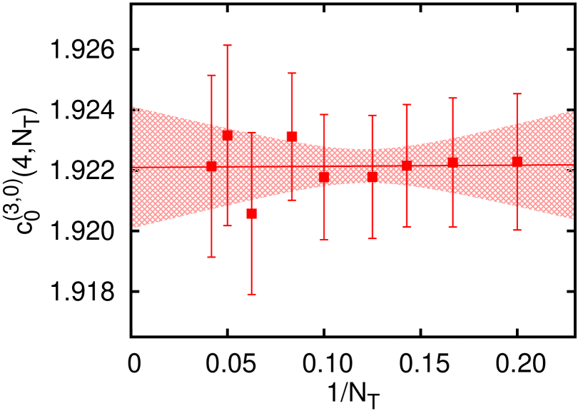
Figure 6: $c^{(3,0)}_{0}(4,N_{T})$ as a function of $1/N_{T}$ compared to a linear fit. The linear term is clearly zero within errors. The fit gives $c^{(3,0)}_{0}(4)=1.9221(20)$, to be compared to $1.92253$ from DLPT, Eqs. (79)–(82).

We now study possible power-suppressed $1/N_{T}$ effects. First we consider the low orders in perturbation theory. At $\mathcal{O}(\alpha)$ the fit function with finite (but large) $N_{T}$ can be obtained with DLPT. No dependence on $N_{T}$ is found. This is also confirmed by our explicit computation of $c_{0}$ with NSPT. We illustrate this for $N_{S}=4$ in Fig. 6. A similar picture applies to the other values of $N_{S}$. The leading terms in $1/N_{S}$ can also be determined using DLPT. Writing

$$c^{(3,0)}_{0}(N_{S},N_{T})=c^{(3,0)}_{0}(N_{S})=c^{(3,0)}_{0}-\frac{f^{(3,0)}_{0}}{N_{S}}-\frac{v^{(3,0)}_{0}}{N^{3}_{S}}+\mathcal{O}\left(\frac{1}{N_{S}^{4}}\right)\,,$$ (79)

we obtain for unsmeared coefficients and TBCxyz boundary conditions

$$c^{(3,0)}_{0,\mathrm{DLPT}} =2.1172743570834807985970\ldots\,,$$ (80)

$$f^{(3,0)}_{0,\mathrm{DLPT}} =0.76962563284(2)\,,$$ (81)

$$v^{(3,0)}_{0,\mathrm{DLPT}} =0.14932(3)\,.$$ (82)

Note that DLPT predicts the absence of an $\mathcal{O}(1/N_{S}^{2})$ term at this order. The above result also applies to the adjoint source, substituting $c^{(8,\rho)}_{0}(N_{S},N_{T})=C_{A}/C_{F}\,c^{(3,\rho)}_{0}(N_{S},N_{T})$, where $C_{A}/C_{F}=2N_{c}^{2}/(N_{c}^{2}-1)=9/4$. We remark that $f_{0}$ and $v_{0}$ depend on the boundary conditions, whereas $c_{0}$ does not.

As we already mentioned, the finite volume $c^{(3,0)}_{0}(N_{S})=c^{(3,0)}_{0}(N_{S},N_{T})$ depend on the boundary conditions. It has previously been computed with PBC, originally in Ref. Heller:1984hx , where intermediate semi-analytic expressions can be found, and in Refs. Nobes:2001tf ; Trottier:2001vj where also TBCxyz and TBCxy boundary conditions were analyzed. No time dependence was found in either case. This absence of a time dependence at $\mathcal{O}(\alpha)$ fits with the spectral picture. The infinite volume coefficient was most precisely computed in Ref. Necco:2001xg . Our determination of $c_{0}$ agrees with the previous results.

At $\mathcal{O}(\alpha^{2})$ we start to encounter a dependence on $N_{T}$. DLPT also gives us information on the coefficient $c_{1}(N_{S},N_{T})$. In this case we have only computed the infinite volume limit for the unsmeared coefficient using the code of Ref. Bali:2002wf in DLPT:

$$c^{(3,0)}_{1,\mathrm{DLPT}}=C_{F}/C_{A}\,c^{(8,0)}_{1,\mathrm{DLPT}}=11.1425(25)\,.$$ (83)

$c^{(3,0)}_{1}$ has been computed previously in a less controlled way using finite Wilson loops Martinelli:1998vt , resulting in the value $c^{(3,0)}_{1}=11.152$. In Ref. Nobes:2001tf agreement with this value was reported. Beyond $\mathcal{O}(\alpha^{2})$ there exist no DLPT results.

 

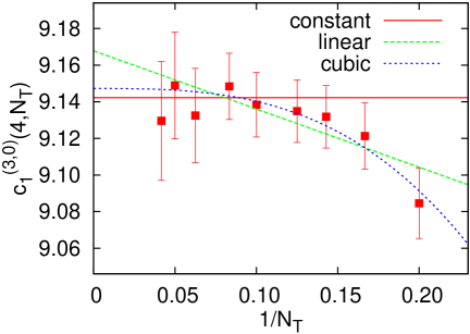
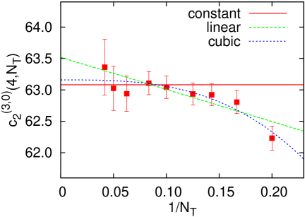
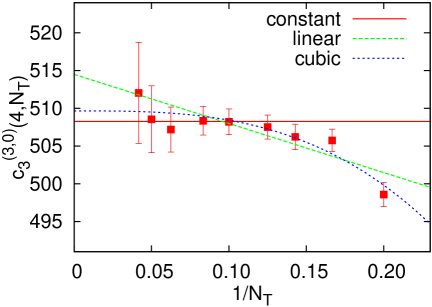
Figure 7: $c^{(3,0)}_{1,2,3}(4,N_{T})$ as a function of $1/N_{T}$, in comparison to a constant plus linear fit, a constant plus cubic fit, and a constant fitted only to the $N_{T}>10$ points.

Next we address NSPT data for $n\geq 1$. We wish to understand the $N_{T}$ dependence for $N_{T}>N_{S}$. For this analysis the simulations to $\mathcal{O}(\alpha^{4})$ at $N_{S}=4$ up to the very high $N_{T}=24$ turn out to be particularly useful. The results are shown in Fig. 7. Note that in these cases the error bars are dominated by the finite Langevin timestep systematics. The $n=1,2,3$ results all show the same qualitative behavior. For $N_{T}\geq 10$ the data are constant within errors, and linear fits result in slopes that are compatible with zero within two standard deviations. For $N_{T}$ smaller than 10 we start to see a bending in $1/N_{T}$, which we parameterize by a $1/N_{T}^{d}$ function. Large powers of $d$ are favored by the fit. The specific power is difficult to determine. We find a $1/N_{T}^{5}$ fit to best describe the data, though only marginally better than a $1/N_{T}^{3}$ fit. Linear $1/N_{T}$ fits, however, are unsatisfactory as we can see in Fig. 7. We can compare the $c^{(3,0)}_{1,2,3}(4,\infty)$-values obtained averaging $N_{T}>10$ data vs. performing $1/N_{T}^{3}$ fits: $9.142\pm 0.012$ vs. $9.147\pm 0.010$, $63.08\pm 0.13$ vs. $63.16\pm 0.10$ and $508.3\pm 1.5$ vs. $509.7\pm 1.0$. Indeed, within our present accuracy, the large-$N_{T}$ data are in agreement with the extrapolation. The same also holds for the smeared and octet data sets.

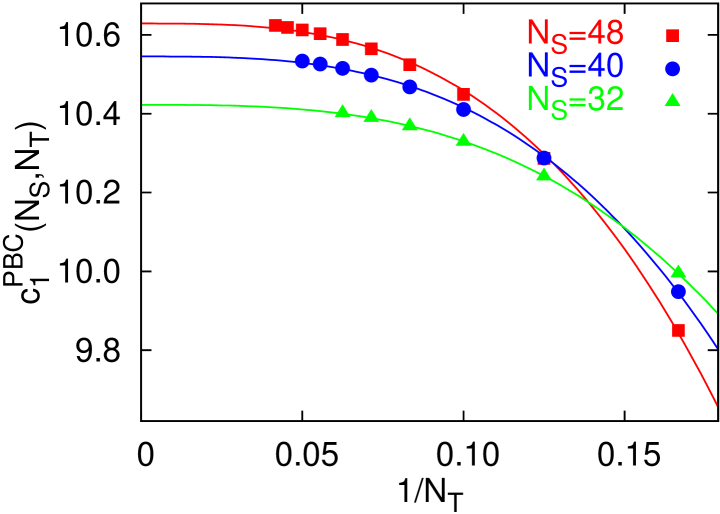
Figure 8: $c^{(3,0)}_{1}(N_{S},N_{T})$ from DLPT obtained on volumes with PBC. The fitted curves are constant plus cubic ($1/N_{T}^{3}$).

We found $1/N_{T}^{5}$ and $1/N_{T}^{3}$ fits to also work well for other $N_{S}$-values (though in these cases we have less data points and therefore less conclusive results). Irrespectively of the power $d$, we observe the coefficient of the $1/N_{T}^{d}$-term to increase roughly linearly with $N_{S}$. From this phenomenological analysis we conclude that the $1/N_{T}$ effects effectively count as $N_{S}/N_{T}^{3}\sim 1/N_{T}^{2}$. Moreover, we find the coefficients of these terms to be numerically small. In order to confirm this phenomenological counting, we have also explored the region $N_{T}\leq N_{S}/2$ for $n=1$ using the PBC DLPT formulae of Ref. Heller:1984hx that only apply to $N_{T}<N_{S}$. In this case for very large volumes ($N_{S}\geq 32$), we indeed found a $(a+bN_{S})/N_{T}^{3}$ parametrization to work well, see Fig. 8. This means that the $1/N_{T}$ effects are clearly subleading, compared to the $1/N_{S}$ effects that we incorporate in our fit and also subleading relative to the unknown $1/N_{S}$ effects starting at $\mathcal{O}(\alpha^{5})$, due to $\beta_{3}$.

While these analyses strongly indicate that the $1/N_{T}$ effects decay rapidly with $N_{T}$, the specific functional form is not exactly known. Therefore, our analysis strategy will be to take $N_{T}\geq\max(N_{S},11)$ so that the $1/N_{T}$ effects can safely be neglected. In this way we loose data and statistics but avoid any bias from assuming a particular functional form. To estimate the cut-off systematics we then vary $N_{T}$ and also consider different trial fit functions. We discuss this issue further in the next section.

Subleading effects of $\mathcal{O}(1/N_{S}^{2})$ would be obscured by the unknown (logarithmically modulated) $1/N_{S}$ effects from higher $\beta$-function coefficients. Therefore we will not consider these.

We conclude with a discussion of lattice artifacts. Formally, we may introduce an anisotropy $a_{t}\neq a_{s}$. In this case the lattice action, that is invariant under time or parity reversal, agrees with the continuum action up to $\mathcal{O}(a_{t}^{2},a_{s}^{2})$-terms. The temporal and spatial lattice extents in physical units are given by $a_{t}N_{T}$ and $a_{s}N_{S}$, respectively, so that the only dimensionless combinations consistent with the leading order lattice artifacts are $a_{t}^{2}/(a_{t}N_{T})^{2}=1/N_{T}^{2}$ and $1/N_{S}^{2}$. Therefore, within perturbation theory, where we cannot dynamically generate additional scales, the LO lattice artifacts are indistinguishable from $\mathcal{O}(1/N_{T}^{2},1/N_{S}^{2})$ finite size effects which, as discussed above, are beyond our present level of precision.

VII Simulation Results

In this section we obtain the infinite volume coefficients of the expansions of four different self-energies: for fundamental and adjoint sources and using static actions with smeared and unsmeared time derivatives. We compare their large order behavior with theoretical expectations, and determine the leading renormalon normalizations $N_{m}$ and $N_{m_{\tilde{g}}}$. We then convert the results into the $\overline{\mathrm{MS}}$ scheme, using different methods, and estimate $\beta_{3}^{\mathrm{latt}}$.

VII.1 Infinite volume coefficients

Below we determine the infinite volume coefficients $c_{n}^{(R,\rho)}$ defined in Eq. (42). Our default fit function for $c^{(R,\rho)}_{n}(N_{S},N_{T})$ (see Eq. (64)) is defined in Eqs. (68)–(70), and depends on the fit parameters $c^{(R,\rho)}_{n}$ and $f^{(R,\rho)}_{j}$ with $j\leq n$. This last dependence introduces a correlation between different $n$-valued coefficients, which we take into account by simultaneously fitting all $c_{n}(N_{S},N_{T})$ to data up to a given order $\mathcal{O}(\alpha^{{n_{\mathrm{max}}}+1})$. By default ${n_{\mathrm{max}}}+1=20$. As a sanity check, we have also fitted each order $n$ independently with two fit parameters $c_{n}$ and $f_{n}$, keeping the $f_{j}$-values that were obtained at previous orders $j<n$ fixed. Since this iterative method does not take account of all correlations, the resulting statistical errors and $\chi^{2}$-values are not reliable. Nevertheless, these fits yield similar central values, illustrating that the low order coefficients are only mildly affected by higher order data. In the following we will only use the results of the global fits.

To ensure that $1/N_{T}$ effects can be neglected we restrict our fits to $N_{T}\geq\max(N_{S},\nu_{T})$ with $\nu_{T}=11$. In addition we restrict $N_{S}\geq\nu_{S}$, varying $\nu_{S}$ to explore the validity range of Eq. (68). Our “thermometer” for this will be to obtain acceptable $\chi^{2}/N_{\mathrm{DF}}$-values and good agreement with $c_{1}^{(3,0)}$ and $c_{1}^{(8,0)}$ from DLPT, Eq. (83). We find that including small volumes improves the quality of the fits: the values of $c_{1}^{(R,0)}$ tend towards the expectations, and $\chi^{2}/N_{\mathrm{DF}}$, as well as the errors, are reduced. We illustrate this behavior in Table 5. We have observed the same behavior for different values of $\nu_{T}$ around 11, and also for the octet and/or smeared perturbative series. Therefore, our default setting will be $\nu_{S}=4$.

Table 5: $\chi^{2}/N_{\mathrm{DF}}$, $c_{1}^{(3,0)}$ and $c_{19}^{(3,0)}$ for different values of $\nu_{S}\leq N_{S}$ ($N_{T}\geq\max(N_{S},11)$). The $n=0$ values were fixed to the DLPT result. Otherwise the $\chi^{2}/N_{\mathrm{DF}}$-values come out even smaller: 1.570, 1.322, 1.209 and 1.152 respectively, whereas the coefficients barely change. The DLPT expectation is $c_{1}^{(3,0)}=11.1425(25)$.

$\nu_{S}$	9	7	6	4
$\chi^{2}/{N_{\mathrm{DF}}}$	1.701	1.431	1.309	1.263
$c_{1}^{(3,0)}$	11.120(33)	11.124(25)	11.122(17)	11.136(11)
$c_{19}^{(3,0)}/10^{23}$	3.919(73)	3.995(55)	4.108(36)	4.118(36)

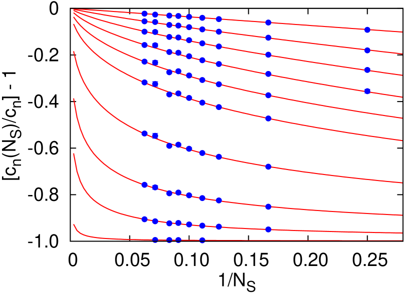
Figure 9: $c^{(3,0)}_{n}(N_{S})/c^{(3,0)}_{n}-1$ for $n\in\{0,1,2,3,4,5,7,9,11,15\}$ (top to bottom). For each value of $N_{S}$ we have plotted the data point with the maximum value of $N_{T}$. The error bars are invisible on the scale of the figure. The curves represent the global fit. For $n=0$ the DLPT prediction $-(1/N_{S})f^{(3,0)}_{0,\mathrm{DLPT}}/c^{(3,0)}_{0,\mathrm{DLPT}}$ of Eqs. (80) and (81) is shown (straight line).

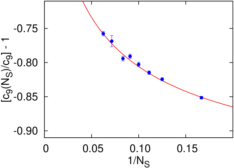
Figure 10: Zoom of Fig. 9 for $n=9$.

The leading parametrical uncertainty stems from the unknown $1/N_{S}$ effects associated to higher order terms in the $\beta$-function: $\beta_{3}$, $\beta_{4}$ etc., which will start affecting the fit at orders $n+1\geq 5$. As long as all singularities of the lattice $\beta$-function in the Borel plane are further away than $u=d/2=1/2$ from the origin (which is the case), these higher $\beta_{i}$ coefficients will not affect the leading renormalon behavior. Nevertheless, there can be an impact at intermediate orders. To study this, for each $c_{n}^{(R,\rho)}(N_{S},N_{T})$ we perform three different fits, setting $\beta_{1}=\beta_{2}=0$ ($\beta_{0}$), setting only $\beta_{2}=0$ ($\beta_{0,1}$), and using all the known coefficients ($\beta_{0,1,2}$). The resulting $c_{n}^{(3,0)}$ are displayed in Table 6 of the Appendix. The results between the $\beta_{0}$ and $\beta_{0,1}$ fits start to deviate from each other significantly at $n=4$ while $\beta_{0,1,2}$ becomes statistically distinguishable from $\beta_{0,1}$ starting around $n=9$. At $n=19$ there is a 25 % variance between the $\beta_{0}$ and $\beta_{0,1,2}$-fits. The convergence pattern is sign alternating. The picture is similar for the smeared and the octet results. We will take the difference between the $\beta_{0,1}$ and $\beta_{0,1,2}$ results as an estimate of the error from subleading terms in the $\beta$-expansion. This is our dominant source of systematic error, by far exceeding, e.g., our statistical errors. We remark that switching off the running altogether ($\beta_{i}=0$) yields a bad $\chi^{2}/N_{\mathrm{DF}}=3.167$ (with $n=0$ fixed from DLPT) and a value of $c^{(3,0)}_{1}$ that is by about 20 standard deviations away from the DLPT result. Once the running is introduced into the parametrization of the finite size effects, these quickly and unavoidably (see Sec. V) grow in size, resulting in large cancellations with the coefficients $c_{n}$. We illustrate the importance of this effect in Fig. 9, where we compare the fitted parametrization to the unsmeared triplet data on $c_{n}(N_{S})/c_{n}-1$ for various $n$ (this also illustrates the quality of the fit). Note that the curvatures, i.e. the deviations from straight lines, are due to the renormalization group running of the $1/N_{S}$ coefficients. The data clearly show the expected curvature. To illustrate this better, we enlarge the $n=9$ curve in Fig. 10.

Next, we estimate the error associated to the $N_{T}$-range dependence that we have not accounted for in our fits. Our data run over a large variety of lattice volumes with different $N_{T}$-values. Our cut-off $N_{T}\geq 11$ eliminates a significant fraction of lattice geometries. However, we can still benefit from these discarded volumes, as they allow us to estimate the systematics associated with our choice of cut-off. We follow two strategies: i) we vary the cut-off $\nu_{T}$. We display $\nu_{T}=9$ results in Table 7. Reducing the cut-off increases the $\chi^{2}/N_{\mathrm{DF}}$-values, since the $1/N_{T}$ curvature is not built into our parametrization. Other than this there is good agreement with our $\nu_{T}=11$ $\beta_{0,1,2}$ fits of Table 6. ii) We introduce a $N_{T}$-dependent term into the fit function in the following way

$$c_{n}(N_{S},N_{T})=c_{n}-\frac{f_{n}(N_{S})}{N_{S}}+\frac{v_{n}(N_{S})}{N_{T}^{d}}\,,$$ (84)

and fit to all our volumes ($\nu_{T}=5$). We have explored different values of $d$ and different parametrizations of $v_{n}(N_{S})$. In Sec. VI the low $n$ $v_{n}(N_{S})$ coefficients were found to increase with $N_{S}$. Global fits also favor this behavior. Therefore, we consider two fit functions: ii.a) $v_{n}(N_{S})/N_{T}^{d}$ where we construct $v_{n}(N_{S})$ in analogy to the $f_{n}(N_{S})$-term, using the renormalization group running of previous orders with just one new fit parameter $v_{n}=v_{n}^{(0)}$ at each order. ii.b) $\tilde{v}_{n}N_{S}/N_{T}^{d}$, assuming a linear dependence of this term on $N_{S}$. We now vary $d$. We take $d=2$ for the ii.a) fit, as we obtain a good $\chi^{2}/N_{\mathrm{DF}}$-value and agreement with $c_{1,\mathrm{DLPT}}$ within one standard deviation. Varying $d$ increases $\chi^{2}/N_{\mathrm{DF}}$ and deteriorates this agreement. We take $d=3$ for the ii.b) fit, as it yields a good $\chi^{2}/N_{\mathrm{DF}}$-value and also perfect agreement with $c_{1,\mathrm{DLPT}}$. $d=2$ results in a difference between the fitted value of $c_{1}$ and $c_{1,\mathrm{DLPT}}$ of several standard deviations, while $d=4$ and $d=5$ reduce the quality of the global fit in terms of the $\chi^{2}$-values.

The $1/N_{T}$ effects are much less constrained by theoretical arguments than the $1/N_{S}$ effects. This could have resulted in a substantial increase of the number of fit parameters necessary to obtain acceptable $\chi^{2}/N_{\mathrm{\mathrm{DF}}}$-values. Fortunately, the $N_{T}$-dependence of the data is much smaller than the $N_{S}$-dependence. We find it remarkable that, with just one additional parameter per order, we can accommodate the complete $N_{T}$ dependence down to $N_{T}=5$. Note that fitting without such an $N_{T}$-term to all volumes $(\nu_{T}=5,\nu_{S}=4)$ we obtain an unacceptable $\chi^{2}/N_{\mathrm{DF}}=3.923$, whereas both choices (ii.a and ii.b) yield good reduced $\chi^{2}$-values, see Table 7. Ansatz ii.b) gives results in perfect agreement with our $\nu_{T}=11$ strategy, while ansatz ii.a) agrees within 1.5 standard deviations. In both cases we fixed the $n=0$ terms from DLPT. We notice that the coefficients $v_{n}$ and $\tilde{v}_{n}$ are small in size and tend to vanish for large $n$, relative to the divergent $c_{n}$ and $f_{n}$.

In spite of this success, we opt for the more conservative strategy of discarding data with $N_{T}<N_{S}$ or $N_{T}<11$, since our $1/N_{T}$-fit ansätze are phenomenological and not fully understood theoretically. For the errors associated to the $N_{T}$-cut, we take the differences between the first columns of Tables 6 and 7, as this choice is completely unbiased regarding the functional form of the $N_{T}$-dependence. We stress that the by far most dominant systematics are the unknown $N_{S}^{-1}\ln^{i}(N_{S})$ terms. Therefore, alternative estimates of the $1/N_{T}$ effect would only marginally affect the final errors.

We have completed the exploration of potential sources of systematic uncertainties. The other perturbative series (smeared, octet and octet smeared) were analyzed analogously, with similar conclusions and precision. In particular similar $\chi^{2}$-values were obtained. The only exception was the octet case, for which we obtained a somewhat reduced precision and the $\chi^{2}$-values were smaller by factors of approximately two. This could be traced to some geometries where the individual errors turned out much bigger. This effect then propagated into the final data set.

We list the final numbers for all the infinite volume coefficients $c_{n}^{(R,\rho)}$ in Table 8. The central values are taken from the first column of Table 6. The quoted errors result from summing statistical and theoretical uncertainties in quadrature. Schematically, we have at each order $n$

$$\sigma_{\mathrm{final}}=\sqrt{\sigma^{2}_{\mathrm{stat.}}+\sigma^{2}_{\beta}+\sigma^{2}_{T}}\,,$$ (85)

where $\sigma_{\beta}$ is the difference between the first and second columns of Table 6, and $\sigma_{T}$ is the difference between the first columns of Tables 6 and 7. We find $\sigma_{\beta}\gg\sigma_{T},\sigma_{\mathrm{stat.}}$, so that the dominant error comes from logarithmic $N_{S}^{-1}\ln^{i}(N_{S})$-corrections, due to our lack of knowledge of $\beta_{3}^{\mathrm{latt}}$ etc.. In comparison to these unknown $1/N_{S}$-terms and the $1/N_{T}^{d}$ corrections addressed above, $1/N_{S}^{2}$ effects are negligible.

In Table 8 we have chosen to multiply the octet coefficients by factors $C_{F}/C_{A}$. In this normalization these will agree with the triplet coefficients for $n=0$ and $n=1$ but at higher orders in general they will differ by $1/N_{c}^{2}$-terms. Within our uncertainties, however, we are unable to resolve these differences.

Our NSPT value $c_{1}^{(3,0)}=11.136(11)$ is in good agreement with the DLPT expectation Eq. (83). $c_{2}^{(3,0)}$ was calculated previously by two groups. One group determined the static energy, singling out the residual mass of the potential using large Wilson loops. Employing NSPT they obtained $c_{2}^{(3,0)}=86.2(0.6)(1.0)$ DiRenzo:2000nd . The second group fitted a polynomial in $\alpha$ to results of non-perturbative simulations of the Polyakov loop at various large values of the inverse lattice coupling $\beta$. They obtained $c_{2}^{(3,0)}=86.6(5)$ Trottier:2001vj . Our result $c_{2}^{(3,0)}=86.10(13)$ confirms these studies, while results for $n>2$ were not known previously, e.g., $c_{3}^{(3,0)}=794.5(1.6)$.

The same analysis also yields the $1/N_{S}$ correction coefficients $f_{n}^{(R,\rho)}$, where we determine the systematic error in the same way as for the $c_{n}^{(R,\rho)}$. We display the results in Table 9.

For large orders the perturbative expansion should be dominated by infrared physics, whereas different smearings correspond to different regularizations of the high energy behavior of the Polyakov loop. Therefore, we expect the smeared and unsmeared coefficients to converge to the same values for large $n$. This is indeed the case for the coefficients $c_{n}$ and $f_{n}$ of both the triplet and octet representations. Actually, the differences between smeared and unsmeared coefficients vanish quite rapidly, around $n=6$ for the $c_{n}$ and already at $n=1$ for the $f_{n}$. Indeed, all smeared and unsmeared values of $f_{n}$ are equal within errors for both representations. This is to be expected, as the coefficients $f_{n}$ are related to finite size effects and know nothing about the specific regularization prescription for the ultraviolet behavior of the Polyakov loop. It is tempting to consider global fits, constraining the smeared and unsmeared $f_{n}$ values to be equal, to increase the accuracy of the results. However, to avoid any bias we will not explore this possibility in this article.

We now move on to determinate the infinite volume $c_{n}/c_{n-1}$-ratios. These are obtained from the same fits, since we have also computed the correlation matrix. Actually, we find strong correlations both of the statistical and systematic errors between consecutive expansion coefficients. Due to these correlations, the infinite volume $c_{n}/c_{n-1}$-ratios can be determined more precisely than the coefficients themselves. The results are displayed in Table 10. Up to $n=11$ the errors increase. For higher orders this tendency is reversed, since the relative impact of the $\beta_{2}$-value (and hence also of the unknown $\beta$-function coefficients) diminishes and so do the effects of finite $N_{T}$-corrections.

As a cross-check we have also determined the coefficients $c_{n}$ by a direct fit to the ratio data

$$\frac{c_{n}}{c_{n-1}}(N_{S},N_{T})\Bigg{|}_{\mathrm{latt.}}=\frac{c_{n}-{f_{n}(N_{S})}/{N_{S}}\quad\left[+{v_{n}(N_{S})}/{N_{T}^{d}}\right]}{c_{n-1}-{f_{n-1}(N_{S})}/{N_{S}}\quad\left[+{v_{n-1}(N_{S})}/{N_{T}^{d}}\right]}\,\,,$$ (86)

using the $f_{0,\mathrm{DLPT}}^{(R,0)}$-value for the non-smeared case and $f_{0,\mathrm{DLPT}}^{(R,1/6)}$, obtained in the previous fit, for the smeared case. For the central values and error estimates we proceed in the same way as we did before. Doing this, overall consistent results and errors for the individual coefficients are found (with slightly bigger $\chi^{2}$-values). The only exception is the unsmeared octet case, where the problems of stability that we already encountered for the $c_{n}$ data become magnified in the ratios, further reducing the precision. Subsequent $c_{n}$-values are statistically correlated and direct fits to the ratio data take these correlations into account. We obtain similar errors and central values as in the previous analysis. This indicates that the statistical correlations of the lattice data do not significantly affect the errors of the infinite volume coefficients, which are dominated by the systematics. As another related cross-check, we have computed the infinite volume $c_{n}/c_{n-1}$ ratios using the ratio data with fit parameters $c_{n}/c_{n-1}$, $f_{n}$ (and $v_{n}$ or $\tilde{v}_{n}$, see the discussion after Eq. (84)), proceeding analogously as above. From this we obtain very similar results to those quoted in Table 10.

Finally, we remark that at the very high orders dominated by the renormalon behavior, TBC cannot and do not reduce finite volume effects, relative to PBC. However, the $v_{n}$- and, at low orders, the $f_{n}$-values are significantly reduced, considerably increasing the robustness of the $c_{n}$- and $f_{n}$-determinations at intermediate and large orders. The effect is twofold. First, the impact of different parametrizations and of the low-$N_{T}$ cut-off value on the $1/N_{T}$-extrapolation is reduced. Second, the low-order $f_{n}$ times $\beta_{3}$ and higher unknown $\beta$-function coefficients that contribute to the $N_{S}^{-1}\ln^{i}(N_{S})$-terms are smaller. Therefore, the uncertainty due to the lack of knowledge of $\beta_{i}$, $i\geq 3$, becomes reduced at intermediate orders (for large $n$ these effects will be small anyhow due to the renormalon dominance, see the discussion around Eq. (77)).

VII.2 Renormalon dominance and the determination of $N_{m}$ and $N_{m_{\tilde{g}}}$

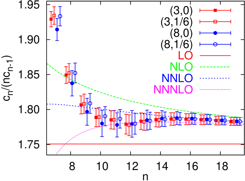
Figure 11: The ratios $c_{n}/(nc_{n-1})$ for the smeared and unsmeared, triplet and octet fundamental static self-energies, compared to the prediction Eq. (59) for the LO, next-to-leading order (NLO), NNLO and NNNLO of the $1/n$ expansion. For clarity, the data sets are slightly shifted horizontally by different off-sets.

In the following we investigate whether the large-$n$ behavior of the four different sets of $c_{n}$ and $f_{n}$ complies with the renormalon expectation and determine the triplet and octet normalizations $N_{m}$ and $N_{m_{\tilde{g}}}$.

In Fig. 11 we compare the $c_{n}/(nc_{n-1})$-ratios summarized in Table 10 to Eq. (59) at different orders in the $1/n$ expansion. The LO and NLO expectations are scheme independent, whereas the NNLO expression depends on the scheme through $\beta_{2}^{\mathrm{latt}}$. For $n\gtrsim 8$ the ratios clearly converge to Eq. (59), and they are within the right ball park of the NNLO prediction, as Fig. 11 illustrates. This is so irrespectively of the representation and smearing, confirming the existence of the renormalon at $d=1$. For completeness, we also plot the NNNLO $\mathcal{O}(1/n^{3})$ expectation, using the $\beta_{3}^{\mathrm{latt}}$ estimate of Eq. (103).

The renormalon picture predicts that $c_{n}\simeq f_{n}$ for large $n$. This equality is achieved with a high degree of accuracy from $n=9$ onwards in all four cases (compare Tables 8 and 9). For the values of $N_{S}$ we explore, the renormalon picture also predicts a strong cancellation between $c_{n}$ and $f_{n}(N_{S})/N_{S}$ for large $n$. We obtain this behavior, which we show in Fig. 9, with an excellent fit to the data (see, for instance, Fig. 10, which is already at an order where renormalon dominance has set in).

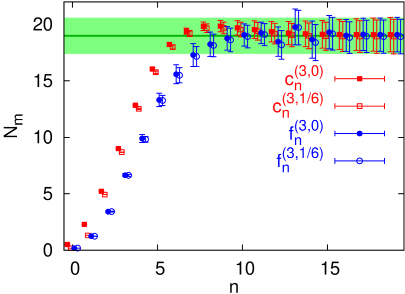
Figure 12: $N_{m}$, determined via Eq. (55), truncated at NNLO, from the coefficients $c_{n}^{(3,0)},c_{n}^{(3,1/6)},f_{n}^{(3,0)}$ and $f_{n}^{(3,1/6)}$. The horizontal band is our final result quoted in Eq. (89).

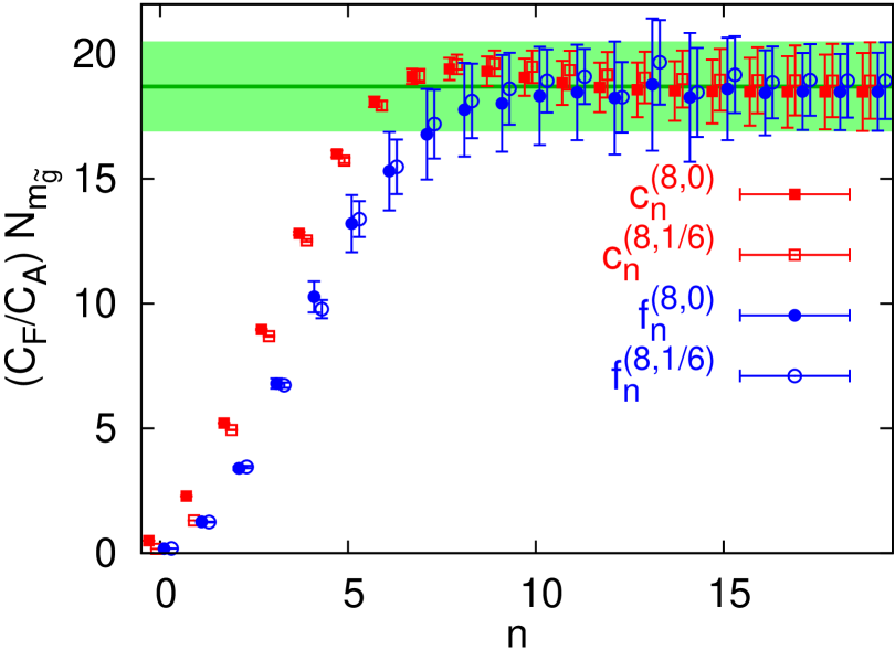
Figure 13: $N_{m_{\tilde{g}}}=-N_{\Lambda}$, determined via Eq. (57), truncated at NNLO, from the coefficients $c_{n}^{(8,0)},c_{n}^{(8,1/6)},f_{n}^{(8,0)}$ and $f_{n}^{(8,1/6)}$. The horizontal band is our final result quoted in Eq. (89). To enable comparison with Fig. 12, we multiply $N_{m_{\tilde{g}}}$ by $C_{F}/C_{A}$.

For each representation $R$ we have four different sequences: $c_{n}^{(R,0)}$, $c_{n}^{(R,1/6)}$, $f_{n}^{(R,0)}$ and $f_{n}^{(R,1/6)}$ that we may use to determine the normalizations $N_{m}$ ($R=3$) and $N_{m_{\tilde{g}}}$ ($R=8$). To obtain the normalizations we divide the large $n$ expectations Eqs. (55) and (57) for the triplet and octet representations by the coefficients obtained in Tables 8 and 9, respectively. We truncate the equations at $\mathcal{O}(1/(n+b))$ precision (NNLO), since resolving the $\mathcal{O}(1/(n+b)^{2})$ correction term requires the knowledge of $\beta_{3}^{\mathrm{latt}}$. For large $n$ these ratios should tend to constants, allowing us to extract $N_{m}$ and $N_{m_{\tilde{g}}}$. This is depicted in Figs. 12 and 13 for triplet and octet sources, respectively. We use the $n=19$ coefficients $c_{19}^{(R,0)}$ and $c_{19}^{(R,1/6)}$, and their associated errors, to obtain the normalizations (recalling that $N_{m_{\tilde{g}}}=-N_{\Lambda}$)

$$N^{\mathrm{latt}}_{m}(\rho=0) =19.1(15)\,,\quad C_{F}/C_{A}\,N^{\mathrm{latt}}_{m_{\tilde{g}}}(\rho=0)=18.5(16)\ ,$$ (87)

$$N^{\mathrm{latt}}_{m}(\rho=1/6) =18.9(15)\,,\quad C_{F}/C_{A}\,N^{\mathrm{latt}}_{m_{\tilde{g}}}(\rho=1/6)=18.9(15)\,.$$ (88)

The errors are much bigger than the differences between the four possible determinations: with or without smearing, using $c_{19}$ or using $f_{19}$. This is not too surprising since these parameters are obtained from one and the same global fit to the same data and hence highly correlated. Moreover, the errors are dominated by the systematics of varying the subleading terms of the finite volume fit function. We obtain our final result by averaging the above central values, with errors that accommodate both the original error bars:

$$N^{\mathrm{latt}}_{m}=19.0\pm 1.6\,,\quad C_{F}/C_{A}\,N^{\mathrm{latt}}_{m_{\tilde{g}}}=18.7\pm 1.8\,.$$ (89)

These numbers are included as error bands into Figs. 12 and 13, respectively. The bands contain all values of the $n\geq 8$ coefficients, lending credibility to our normalization estimates. Note that, on general grounds, we would expect the ratio $N_{\tilde{m}}/N_{m}$ to differ from the Casimir scaling factor $C_{A}/C_{F}$ by an $\mathcal{O}(1/N_{c}^{2})$-term, which naively amounts to 10%, roughly the level of our accuracy. We discuss this issue further in the next subsection.

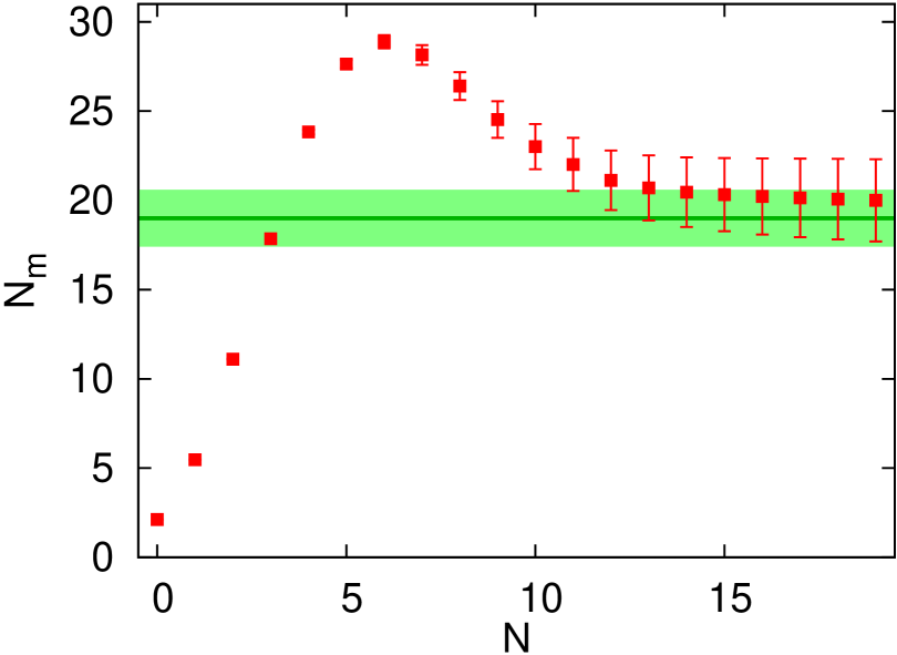
Figure 14: $N_{m}$, determined from the coefficients $c_{n}^{(3,0)}$, $n\leq N$, using Eq. (92). The error band corresponds to the result Eq. (89).

As a cross-check we also estimate the normalization from the Borel transform of the static energy perturbative series

$$B^{(N)}[\delta m](t(u))=\sum_{n=0}^{N}\frac{c_{n}}{n!}\left(\frac{4\pi}{\beta_{0}}u\right)^{n}\,,$$ (90)

using the function

$$D^{(N)}_{m}(u) =\sum_{n=0}^{N}D_{m}^{(n)}u^{n}=(1-2u)^{1+b}B^{(N)}[\delta m](t(u))$$ (91)

$$=N_{m}\frac{1}{a}\left(1+c_{1}(1-2u)+c_{2}(1-2u)^{2}+\cdots\right)+(1-2u)^{1+b}({\rm analytic\;term})\,,$$

as it was first done in Ref. Pineda:2001zq for the pole mass, using ideas developed in Refs. Lee:1996yk ; Lee:1999ws . $D^{(N)}_{m}(u)$ is singular but bounded at the first IR renormalon. Therefore, we can estimate $N_{m}$ from the first coefficients of the series in $u$, using

$$N^{(N)}_{m}\frac{1}{a}=D^{(N)}_{m}(u=1/2)\,.$$ (92)

We plot the predictions for different orders $N$ in Fig. 14. The error is propagated from the error of the coefficient. Within one standard deviation the result is consistent with Eq. (89) (error band), though less precise.

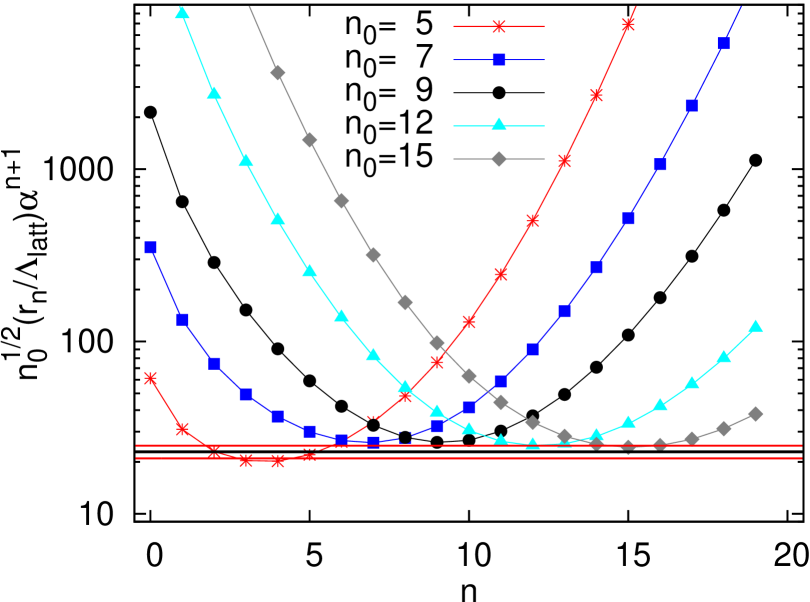
Figure 15: Eq. (93) times $\sqrt{n_{0}}$, for five different values of the lattice scheme coupling constant $\alpha$, ranging from $\alpha(\nu)\approx 0.096$ ($n_{0}=5$) to $\alpha(\nu)\approx 0.036$ ($n_{0}=15$). The error band corresponds to the estimate of Eq. (62), where we have used the value $N_{m}=19.0\pm 1.6$ [Eq. (89)].

Finally, we show in Fig. 15 the divergent behavior of the perturbative expansion of the pole mass, Eq. (43). We use the fact that $r_{n}=\nu c_{n}^{(3,0)}$ for large $n$ and the coefficients listed in Table 8. We compute

$$\frac{r_{n}}{\Lambda_{\mathrm{latt}}}\alpha^{n+1}(\nu)=c_{n}\alpha^{n+1}(\nu)\exp\!\left(\frac{2\pi}{\beta_{0}\alpha(\nu)}\right)\left(\frac{\beta_{0}\alpha(\nu)}{4\pi}\right)^{\!\!b}+\cdots\,,$$ (93)

where we truncate Eq. (49) at two-loop order. In Fig. 15 we plot Eq. (93) times $\sqrt{n_{0}}$ (see Eq. (62)) as a function of $n$ for $\alpha\approx 0.096,0.072,0.057,0.044$ and 0.036. These values are chosen so that the minimal term in the two-loop approximation of Eq. (60) corresponds to $n_{0}=5,7,9,12$ and 15, respectively. In terms of the inverse lattice coupling parameter $\beta=3/(2\pi\alpha)$ this covers the range $4.97\lesssim\beta\lesssim 13.32$. Orders $n_{0}=6,7$ ($\beta\approx 5.8,6.6$) are typical for present-day non-perturbative lattice simulations, with inverse lattice spacings $1.5\,\mathrm{GeV}\lesssim a^{-1}\lesssim 5.2\,\mathrm{GeV}$ Necco:2001xg , while the $n_{0}=5$ value is in the strong coupling regime. As expected, the contributions to the sum decrease monotonously down to an order $\sim\alpha^{n_{0}+1}$, before starting to diverge exponentially. The horizontal error band corresponds to the uncertainty, estimated in Eq. (62), of the sum truncated at order $n_{0}$

$$\sqrt{n_{0}}\frac{|r_{n_{0}}|}{\Lambda_{\mathrm{latt}}}\alpha^{n_{0}+1}(\nu)=\frac{2^{3/2-b}\pi^{3/2}}{\beta_{0}\Gamma{(1+b)}}|N_{m}|\approx 1.206\,|N_{m}|\,,$$ (94)

where we used the value $N_{m}=19.0\pm 1.6$ [Eq. (89)]. Using $\Lambda_{\mathrm{latt}}\approx 8.2~{}\mathrm{MeV}$ Capitani:1998mq , this horizontal line corresponds to about 190 MeV. The data are very consistent with expectations, the only difference being that at the largest coupling (lowest scale $\nu$) the order of the minimal term is somewhat lower than expected ($n_{0}=3,4$ instead of $n_{0}=5$). We obtain very similar results from the smeared and the octet data.

At smaller $\alpha$, i.e. at higher $\nu$, the minimal term $c_{n_{0}}\alpha^{n_{0}+1}(\nu)$ is numerically smaller than at lower scales. However, this is compensated for by the linear divergence of $r_{n}=\nu c_{n}$, resulting in a similar overall uncertainty. The only difference is that to achieve this accuracy, at higher scales one has to expand to higher orders.

VII.3 Conversion to the $\overline{\mathrm{MS}}$ scheme and determination of $\beta_{3}^{\mathrm{latt}}$

The results of the infinite volume coefficients $c_{n}^{(R,\rho)}$, $N_{m}$ and $N_{m_{\tilde{g}}}$ presented above have been obtained in the (Wilson) lattice scheme. Translating a coefficient $c_{n}^{(R,\rho)}$ to a different scheme would require the knowledge of the conversion to order $\alpha^{n+1}$. This is completely beyond reach. For the case of $\overline{\mathrm{MS}}$, the conversion

$$\alpha_{\overline{\mathrm{MS}}}(\mu)=\alpha_{\mathrm{latt}}(\mu)\left(1+d_{1}\alpha_{\mathrm{latt}}(\mu)+d_{2}\alpha^{2}_{\mathrm{latt}}(\mu)+d_{3}\alpha^{3}_{\mathrm{latt}}(\mu)+\mathcal{O}(\alpha_{\mathrm{latt}}^{4})\right)\,,$$ (95)

is known to two loops with Hasenfratz:1980kn ; Weisz:1980pu ; Luscher:1995np $d_{1}=5.88359144663707(1)$ and Luscher:1995np ; Christou:1998ws ; Bode:2001uz $d_{2}=43.4073028(2)$. Fortunately, only $d_{1}$ is needed to determine the ratio of $\Lambda$-parameters, and $N^{\overline{\mathrm{MS}}}_{m}$ and $N^{\overline{\mathrm{MS}}}_{m_{\tilde{g}}}$, since (exactly!)

$$N^{\overline{\mathrm{MS}}}_{m,m_{\tilde{g}}}=N^{\mathrm{latt}}_{m,m_{\tilde{g}}}\Lambda_{\mathrm{latt}}/\Lambda_{\overline{\mathrm{MS}}}\,,\quad\mbox{where}\quad\Lambda_{\overline{\mathrm{MS}}}=e^{\frac{2\pi d_{1}}{\beta_{0}}}\Lambda_{\mathrm{latt}}\approx 28.809338139488\,\Lambda_{\mathrm{latt}}\,.$$ (96)

This yields the numerical values

$$N^{\overline{\mathrm{MS}}}_{m}=0.660(56)\,,\quad C_{F}/C_{A}\,N^{\overline{\mathrm{MS}}}_{m_{\tilde{g}}}=-C_{F}/C_{A}\,N^{\overline{\mathrm{MS}}}_{\Lambda}=0.649(62)\,.$$ (97)

Other combinations of interest are (see Eqs. (56) and (58))

$$N^{\overline{\mathrm{MS}}}_{V_{s}}=-1.32(11)\,,\quad N^{\overline{\mathrm{MS}}}_{V_{o}}=0.14(18)\,.$$ (98)

These results can be compared to previous determinations from continuum computations in the $\overline{\mathrm{MS}}$ scheme Pineda:2002se ; Lee:2002sn ; Bali:2003jq ; Brambilla:2010pp . The agreement is remarkably good, which is highly nontrivial given the factor $\simeq 29$ between the values of $N_{m}$ and $N_{\Lambda}$ in both schemes, due to the big difference between the $\Lambda_{\overline{\mathrm{MS}}}$- and $\Lambda_{\mathrm{latt}}$-parameters, i.e., the large value of $d_{1}$. Moreover, in the $\overline{\mathrm{MS}}$ scheme the normalization was determined from the first few terms of the perturbative series only, while in the lattice scheme $n\geq 9$ was required. As expected, the onset of the renormalon dominated behavior depends on the scheme. Nowadays, several diagrammatic continuum perturbation theory computations in heavy quark physics have reached a level of precision where they become sensitive to the leading renormalon. We remark that there has always been some doubt about the reliability of determinations of $N^{\overline{\mathrm{MS}}}_{m}$ and $N^{\overline{\mathrm{MS}}}_{\Lambda}$ from just very few orders of perturbation theory. We have now provided an entirely independent determination of these objects based on many orders of the expansion that can systematically be improved upon. Our quenched result presented here goes beyond the present state-of-the-art. An analogous un-quenched determination could give similarly precise values for $N^{\overline{\mathrm{MS}}}_{m}$ and $N^{\overline{\mathrm{MS}}}_{\Lambda}$, with direct consequences to heavy quark physics, e.g., if using the $\mathrm{RS}$ scheme Pineda:2001zq .

To further support our conclusions, we convert the $c_{n}(N_{S},N_{T})$ lattice coefficients, and their ratios, into the $\overline{\mathrm{MS}}$ scheme. As we have already mentioned, we can only exactly perform this conversion up to $n=2$. For $n>2$ the $\overline{\mathrm{MS}}$ coefficients and ratios will depend on the approximation used. If the renormalon picture is correct, the large-$n$ ratios should be dominated by the renormalon behavior and all ”$\overline{\mathrm{MS}}$-like” conversions should yield similar results. However, coefficients and ratios at intermediate orders will depend on the approximation used. We consider two different $\overline{\mathrm{MS}}$-like conversion schemes:
(a) $\overline{\mathrm{MS}}_{a}$

$$\alpha_{\mathrm{latt}}(\mu)=\alpha_{\overline{\mathrm{MS}}}(\mu)\frac{1}{1+d_{1}\alpha_{\overline{\mathrm{MS}}}(\mu)+(d_{2}-d_{1}^{2})\alpha^{2}_{\overline{\mathrm{MS}}}(\mu)}\ ,$$ (99)

(b) $\overline{\mathrm{MS}}_{b}$

$$\alpha_{\mathrm{latt}}(\mu)=\alpha_{\overline{\mathrm{MS}}}(\mu)\left(1-d_{1}\alpha_{\overline{\mathrm{MS}}}(\mu)+(2d_{1}^{2}-d_{2})\alpha^{2}_{\overline{\mathrm{MS}}}(\mu)\right)\ .$$ (100)

We suspect the scheme $\overline{\mathrm{MS}}_{a}$ to be superior, since the translation of $1/\alpha$ rather than of $\alpha$ from one scheme to another generates a renormalization group-like resummation.

Our statistical data analysis Wolff:2003sm allows for the direct evaluation of derived/secondary observables. The expansion of the logarithm of the Polyakov loop is the most obvious secondary observable and produces the coefficients $c_{n}(N_{S},N_{T})$, but we can also intertwine the logarithm with other functions, such as the change from the lattice to a $\overline{\mathrm{MS}}$-like scheme. We do so using Eqs. (99) and (100). In addition, we employ DLPT to obtain $c^{(3,0)}_{1,\overline{\mathrm{MS}}}=C_{F}/C_{A}\,c^{(8,0)}_{1,\overline{\mathrm{MS}}}=-1.3147(25)$, whereas the first coefficient $c_{0}$ is scheme independent.

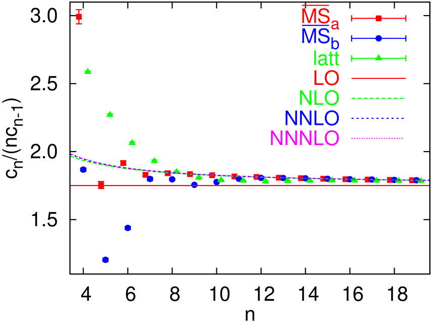
Figure 16: The ratio $c^{(3,0)}_{n}/(nc^{(3,0)}_{n-1})$ in the lattice and $\overline{\mathrm{MS}}$-like schemes, compared to the prediction Eq. (59). NNLO and NNNLO refer to the respective $\overline{\mathrm{MS}}$ scheme expectations.

In Fig. 16 we show our determination of $c^{(3,0)}_{n}/(nc^{(3,0)}_{n-1})$ using the two $\overline{\mathrm{MS}}$-like conversions (a) and (b). We only display the statistical errors associated to the fit. We have not performed a complete error analysis, as the $\overline{\mathrm{MS}}$-like conversions introduce unknown systematics. As anticipated, both $\overline{\mathrm{MS}}$-like schemes converge to the renormalon expectation. Actually, leaving aside systematic errors, it converges to the $\overline{\mathrm{MS}}$ NNLO expectation rather than the lattice one. For the more stable $\overline{\mathrm{MS}}_{a}$ scheme, renormalon dominance sets in already at orders $n\sim 5,6$, significantly earlier than in the lattice scheme.

Following the analysis of the Sec. VII.2, we can determine the normalization of the renormalon from the coefficient $c_{19}$, obtaining the estimates

$$N_{m}^{\overline{\mathrm{MS}}_{a}}\simeq 0.51\ ,\qquad N_{m}^{\overline{\mathrm{MS}}_{b}}\simeq 1.53\,,$$ (101)

to be compared to the correct value $N_{m}^{\overline{\mathrm{MS}}}=0.66(6)$ of Eq. (97). Of course, due to the mismatch at intermediate orders, these numbers are not trustworthy. However, considering the $\mathcal{O}(10^{22})$ size of $c_{19}$, the numbers certainly are within the right ball park. As expected, the scheme $\overline{\mathrm{MS}}_{a}$ is superior, both in terms of an earlier onset of the asymptotic behavior and the extracted value of the normalization $N_{m}^{\overline{\mathrm{MS}}_{a}}\simeq N_{m}^{\overline{\mathrm{MS}}}$. A similar picture is obtained for all the other sequences except for the unsmeared octet. In this latter case the data become too noisy to obtain stable results.

Since we know $\beta_{3}^{\overline{\mathrm{MS}}}$ vanRitbergen:1997va , we can go one order higher in $1/n$ in the prediction for the ratios and coefficients of the $\overline{\mathrm{MS}}$-like schemes. Incorporating the running to this higher order into the fit function produces very small shifts of the predicted ratios and coefficients. This confirms that introducing consecutive orders of the $\beta$-function into the fit leads to a convergent parametrization of the $c_{n}$ coefficients and associated ratios.

The previous fits indicate that the asymptotic behavior of the ratios is not very sensitive to their values at intermediate orders. However, the normalization $N_{m}$ is, as the value of a high order coefficient $c_{n}$, obtained from a global fit will, through the running of the $1/N_{S}$ finite size effect, also depend on $n$-intermediate orders. This is also so if one tries to obtain the coefficients $c_{n}$ through the ratios. The reason is that these are determined from the relation $c_{n}=c_{0}\Pi_{j=1}^{n}\frac{c_{j}}{c_{j-1}}$, which is sensitive to the intermediate values of $\frac{c_{j}}{c_{j-1}}$. In spite of these caveats the results are encouraging and perfectly compatible with expectations.

We expect that the renormalon dominance of the static energy expansion sets in at much lower orders in the $\overline{\mathrm{MS}}$ scheme than in the lattice scheme. This is supported by the consistency of our $N_{m}$-determination with continuum estimates that are based on only a few orders. Also the earlier onset of the asymptotics in the $\overline{\mathrm{MS}}$-like schemes is coherent with this assumption. We can turn this argument around to estimate $d_{3}$ [cf. Eq. (95)] and $\beta_{3}^{\mathrm{latt}}$, assuming that

$$c_{3,\overline{\mathrm{MS}}}\simeq N^{\overline{\mathrm{MS}}}_{m}\,\left(\frac{\beta_{0}}{2\pi}\right)^{3}\,\frac{\Gamma(4+b)}{\Gamma(1+b)}\left(1+\frac{b}{(3+b)}s_{1}+\frac{b(b-1)}{(3+b)(2+b)}s_{2}+\cdots\right).$$ (102)

Using our central value $c_{3,\mathrm{latt}}^{(3,0)}=794.5$, we obtain

$$d_{3}\simeq 365\,,\qquad\beta_{3}^{\mathrm{latt}}\simeq-1.7\times 10^{6}\,.$$ (103)

Eq. (102) introduces a systematic error that is difficult to estimate. Nevertheless, we have checked that the value of $d_{3}$ varies at the few per mille level when considering the uncertainties of $N_{m}$, $c_{3,\mathrm{latt}}^{(3,0)}$, or when truncating Eq. (102) at a lower order in $1/n$. This translates into variations at the level of a few per cent for $\beta_{3}^{\mathrm{latt}}$. We have also checked that introducing this estimate of $\beta_{3}^{\mathrm{latt}}$ in our fit function of Sec. VII.1 yields a convergent pattern (in the number of $\beta$-coefficients included) for $c_{n}$ and $c_{n}/(nc_{n-1})$. In this case $c_{n}/(nc_{n-1})$ converges to Eq. (59) with NNNLO precision. The fit produces a somewhat smaller value of $N_{m}$ that agrees within one standard deviation with the result stated in Eq. (89).

VIII Conclusions

We have determined the infinite volume coefficients of the perturbative expansions of the self-energies of static sources in the fundamental and adjoint representations to $\mathcal{O}(\alpha^{20})$ in gluodynamics. We have employed lattice regularization with the Wilson action and two different discretizations of the covariant time derivative of the Polyakov loop. The computation was performed using NSPT. Overall, we have obtained the infinite volume coefficients of four different perturbative series, which we show in Table 8. At high orders all series display the factorial growth predicted by the conjectured renormalon picture based on the operator product expansion. This can also nicely be seen from the normalized ratios of subsequent coefficients $c_{n}/(nc_{n-1})$, which converge to Eq. (59) for large $n$, as can be read off from Table 10. The coefficients that govern spatial finite size effects, $f_{n}$, also grow factorially, as predicted by the renormalon dominance picture, see Table 9.

Furthermore, we have determined the normalization constant of the first infrared renormalon of a heavy quark pole mass and of the gluelump mass:

$$N^{\mathrm{latt}}_{m} =19.0\pm 1.6\,,\quad C_{F}/C_{A}\,N^{\mathrm{latt}}_{\Lambda}=-18.7\pm 1.8\,,$$ (104)

$$N^{\overline{\mathrm{MS}}}_{m} =0.660\pm 0.056\,,\quad C_{F}/C_{A}\,N^{\overline{\mathrm{MS}}}_{\Lambda}=-0.649\pm 0.062\,.$$ (105)

We stress that the $N_{m}$-value is more than ten standard deviations different from zero, proving, with this significance, the existence of the $d=1$ renormalon in gluodynamics. We also find it remarkable that we can obtain a result in a continuum scheme directly (and exactly) from a computation in lattice regularization, with no error in the conversion.

The above numbers are in agreement, within errors, with determinations from continuum-like computations, but they have been obtained using completely independent methods. In particular, for the first time, it was possible to follow the factorial growth of the coefficients over many orders, from around $\alpha^{9}$ up to $\alpha^{20}$, vastly increasing the credibility of the prediction. The results of this article can be used to predict higher order terms of the heavy quark pole mass, of the static singlet and hybrid potentials and of the heavy gluino pole mass (gluelump) expansions. Unfortunately, at present, for the latter we do not have sufficient precision to discriminate Casimir scaling violation effects, suppressed by $1/N_{c}^{2}$ in the number of colors.

Our precision is mainly limited by our knowledge of the fit function, and in particular of $\beta_{3}^{\mathrm{latt}}$. We have been able to estimate its value, $\beta_{3}^{\mathrm{latt}}\simeq-1.7\times 10^{6}$, assuming that the renormalon dominance in the $\overline{\mathrm{MS}}$ scheme sets in around $\mathcal{O}(\alpha^{4})$. However, an independent precise determination would further decrease the errors of the infinite volume coefficients and of the normalizations $N_{m}$ and $N_{m_{\tilde{g}}}$. Performing simulations on larger lattice volumes would also be desirable, to further improve the control of finite size effects. However, the statistical noise increases substantially with the length of the Polyakov loop $N_{T}$ and we find simulations to become unstable for asymmetries $N_{S}\gg N_{T}$. This behavior deserves further study.

While the addition of a small number of quark flavors will neither affect any of the qualitative conclusions presented here nor the renormalon structure of the theory, a similar un-quenched analysis would be very important. This would provide a reliable, independent determination of $N^{\overline{\mathrm{MS}}}_{m}$, including the effect of light flavors, with major impact on renormalon analyses in heavy quark physics and, in particular, enabling more accurate determinations of the heavy quark masses, including that of the top quark.

Appendix A Tables

Table 6: Fit of $c_{n}^{(3,0)}$ with different approximations to the $\beta$-function. $c^{(3,0)}_{0}$ and $f^{(3,0)}_{0}$ were fixed to the DLPT result. Leaving these parameters free slightly decreases the $\chi^{2}/N_{\mathrm{DF}}$-values to 1.111,1.152,1.177 respectively, without significant changes in any of the fit parameters.

	$\beta_{0,1,2}$	$\beta_{0,1}$	$\beta_{0}$
$\chi^{2}/N_{\mathrm{DF}}$	1.263	1.290	1.218
$c_{1}/10$	1.1136(11)	1.1136(11)	1.1136(11)
$c_{2}/10$	8.610(13)	8.610(13)	8.597(13)
$c_{3}/10^{2}$	7.945(14)	7.951(14)	7.914(14)
$c_{4}/10^{3}$	8.215(26)	8.232(26)	8.156(26)
$c_{5}/10^{4}$	9.322(40)	9.361(40)	9.203(40)
$c_{6}/10^{6}$	1.1533(61)	1.1619(61)	1.1292(61)
$c_{7}/10^{7}$	1.5576(96)	1.5760(96)	1.5067(94)
$c_{8}/10^{8}$	2.304(16)	2.345(16)	2.194(15)
$c_{9}/10^{9}$	3.747(27)	3.837(27)	3.499(25)
$c_{10}/10^{10}$	6.702(49)	6.913(50)	6.121(46)
$c_{11}/10^{12}$	1.3160(98)	1.367(10)	1.1740(89)
$c_{12}/10^{13}$	2.809(24)	2.939(24)	2.446(21)
$c_{13}/10^{14}$	6.513(56)	6.855(58)	5.537(51)
$c_{14}/10^{16}$	1.628(14)	1.723(15)	1.353(13)
$c_{15}/10^{17}$	4.363(38)	4.641(40)	3.546(33)
$c_{16}/10^{19}$	1.247(11)	1.332(11)	0.9925(92)
$c_{17}/10^{20}$	3.785(33)	4.059(35)	2.953(28)
$c_{18}/10^{22}$	1.215(11)	1.308(11)	0.930(09)
$c_{19}/10^{23}$	4.118(36)	4.446(38)	3.094(29)

Table 7: Determination of $c_{n}^{(3,0)}$ using the methods i), ii.a), and ii.b) explained around Eq. (84) of Sec. VII.1. The first column is the result of a fit with two parameters per order [Eq. (68)] to the $N_{T}\geq\max(N_{S},9)$ geometries. The analogous $N_{T}\geq\max(N_{S},11)$ results are displayed in the first column of Table 6. The second and third columns are from fits of Eq. (84) to all volumes, with one extra fit parameter per order: in the second column we set $d=2$ and obtain $v_{n}(N_{S})$ from the renormalization group running using $\beta_{0},\beta_{1},\beta_{2}$ and results from previous orders $v_{n-1}^{(0)}$ etc.. In the last column we set $d=3$ and $v_{n}(N_{S})=\tilde{v}_{n}N_{S}$.

	$\nu_{T}=9$	$v_{n}(N_{S})/N_{T}^{2}$	$\tilde{v}_{n}N_{S}/N_{T}^{3}$
$\chi^{2}/N_{\mathrm{DF}}$	1.666	0.940	1.033
$c_{1}/10$	1.1133(10)	1.11360(89)	1.11442(89)
$c_{2}/10$	8.607(12)	8.612(10)	8.619(10)
$c_{3}/10^{2}$	7.940(12)	7.944(10)	7.947(10)
$c_{4}/10^{3}$	8.201(24)	8.233(22)	8.231(22)
$c_{5}/10^{4}$	9.305(37)	9.361(34)	9.340(35)
$c_{6}/10^{6}$	1.1512(56)	1.1606(52)	1.1551(53)
$c_{7}/10^{7}$	1.5549(88)	1.5706(81)	1.5589(83)
$c_{8}/10^{8}$	2.301(14)	2.328(13)	2.305(13)
$c_{9}/10^{9}$	3.742(24)	3.791(23)	3.745(23)
$c_{10}/10^{10}$	6.695(45)	6.790(41)	6.695(43)
$c_{11}/10^{12}$	1.3144(89)	1.3341(82)	1.3137(85)
$c_{12}/10^{13}$	2.812(20)	2.850(19)	2.805(19)
$c_{13}/10^{14}$	6.526(48)	6.607(44)	6.490(45)
$c_{14}/10^{16}$	1.632(12)	1.652(11)	1.620(11)
$c_{15}/10^{17}$	4.375(33)	4.426(30)	4.340(31)
$c_{16}/10^{19}$	1.2506(94)	1.2650(85)	1.2401(88)
$c_{17}/10^{20}$	3.796(28)	3.839(26)	3.764(27)
$c_{18}/10^{22}$	1.2192(92)	1.2331(83)	1.2087(86)
$c_{19}/10^{23}$	4.130(31)	4.177(28)	4.094(29)

Table 8: The infinite volume coefficients $c_{n}^{(R,\rho)}$, including all systematic errors. The unsmeared $c_{0}$-values are fixed using DLPT.

	$c_{n}^{(3,0)}$	$c_{n}^{(3,1/6)}$	$c_{n}^{(8,0)}C_{F}/C_{A}$	$c_{n}^{(8,1/6)}C_{F}/C_{A}$
$c_{0}$	2.117274357	0.72181(99)	2.117274357	0.72181(99)
$c_{1}$	11.136(11)	6.385(10)	11.140(12)	6.387(10)
$c_{2}/10$	8.610(13)	8.124(12)	8.587(14)	8.129(12)
$c_{3}/10^{2}$	7.945(16)	7.670(13)	7.917(20)	7.682(15)
$c_{4}/10^{3}$	8.215(34)	8.017(33)	8.197(42)	8.017(36)
$c_{5}/10^{4}$	9.322(59)	9.160(59)	9.295(76)	9.139(64)
$c_{6}/10^{6}$	1.153(11)	1.138(11)	1.144(13)	1.134(12)
$c_{7}/10^{7}$	1.558(21)	1.541(22)	1.533(25)	1.535(22)
$c_{8}/10^{8}$	2.304(43)	2.284(45)	2.254(51)	2.275(45)
$c_{9}/10^{9}$	3.747(95)	3.717(97)	3.64(11)	3.703(98)
$c_{10}/10^{10}$	6.70(22)	6.65(22)	6.49(25)	6.63(22)
$c_{11}/10^{12}$	1.316(52)	1.306(53)	1.269(59)	1.303(53)
$c_{12}/10^{13}$	2.81(13)	2.79(13)	2.71(14)	2.78(13)
$c_{13}/10^{14}$	6.51(35)	6.46(35)	6.29(37)	6.45(35)
$c_{14}/10^{16}$	1.628(96)	1.613(97)	1.57(10)	1.614(97)
$c_{15}/10^{17}$	4.36(28)	4.32(28)	4.22(29)	4.33(28)
$c_{16}/10^{19}$	1.247(86)	1.235(86)	1.206(89)	1.236(86)
$c_{17}/10^{20}$	3.78(28)	3.75(28)	3.66(28)	3.75(28)
$c_{18}/10^{22}$	1.215(93)	1.204(94)	1.176(95)	1.205(94)
$c_{19}/10^{23}$	4.12(33)	4.08(33)	3.99(34)	4.08(33)

Table 9: The $1/N_{S}$ correction coefficients $f_{n}^{(R,\rho)}$, including all systematic errors. The unsmeared $f_{0}$-values are fixed using DLPT.

	$f_{n}^{(3,0)}$	$f_{n}^{(3,1/6)}$	$f_{n}^{(8,0)}C_{F}/C_{A}$	$f_{n}^{(8,1/6)}C_{F}/C_{A}$
$f_{0}$	0.7696256328	0.7810(59)	0.7696256328	0.7810(69)
$f_{1}$	6.075(78)	6.046(58)	6.124(87)	6.063(68)
$f_{2}/10$	5.628(91)	5.644(62)	5.60(11)	5.691(78)
$f_{3}/10^{2}$	5.87(11)	5.858(76)	6.00(18)	5.946(91)
$f_{4}/10^{3}$	6.33(22)	6.29(17)	6.57(40)	6.26(23)
$f_{5}/10^{4}$	7.73(35)	7.71(26)	7.67(66)	7.78(42)
$f_{6}/10^{5}$	9.86(53)	9.80(42)	9.68(99)	9.79(69)
$f_{7}/10^{7}$	1.388(81)	1.378(71)	1.35(15)	1.38(11)
$f_{8}/10^{8}$	2.12(12)	2.11(12)	2.06(22)	2.10(17)
$f_{9}/10^{9}$	3.54(20)	3.52(20)	3.40(37)	3.51(27)
$f_{10}/10^{10}$	6.49(33)	6.44(34)	6.23(67)	6.44(43)
$f_{11}/10^{12}$	1.296(64)	1.286(66)	1.24(13)	1.286(74)
$f_{12}/10^{13}$	2.68(19)	2.64(18)	2.65(33)	2.65(21)
$f_{13}/10^{14}$	6.70(54)	6.68(52)	6.36(90)	6.66(57)
$f_{14}/10^{16}$	1.58(14)	1.56(14)	1.55(22)	1.57(15)
$f_{15}/10^{17}$	4.41(34)	4.37(33)	4.24(47)	4.37(35)
$f_{16}/10^{19}$	1.241(92)	1.230(91)	1.20(11)	1.231(94)
$f_{17}/10^{20}$	3.79(28)	3.75(28)	3.67(30)	3.76(28)
$f_{18}/10^{22}$	1.215(94)	1.204(94)	1.176(97)	1.205(94)
$f_{19}/10^{23}$	4.12(33)	4.08(33)	3.99(34)	4.08(33)

Table 10: The infinite volume ratios $c_{n}^{(R,\rho)}/\left(nc_{n-1}^{(R,\rho)}\right)$, including all systematic errors. Note that $\beta_{0}/(2\pi)\approx 1.7507$.

$n$	$c_{n}^{(3,0)}/\left(nc_{n-1}^{(3,0)}\right)$	$c_{n}^{(3,1/6)}/\left(nc_{n-1}^{(3,1/6)}\right)$	$c_{n}^{(8,0)}/\left(nc_{n-1}^{(8,0)}\right)$	$c_{n}^{(8,1/6)}/\left(nc_{n-1}^{(8,1/6)}\right)$
1	5.2594(47)	8.8462(60)	5.2616(56)	8.8480(61)
2	3.8662(30)	6.3613(39)	3.8539(36)	6.3641(41)
3	3.0756(41)	3.1474(42)	3.0735(53)	3.1500(45)
4	2.5850(69)	2.6129(76)	2.5884(94)	2.6091(79)
5	2.2695(81)	2.2851(90)	2.268(13)	2.280(11)
6	2.0621(96)	2.071(11)	2.051(15)	2.069(13)
7	1.929(11)	1.934(13)	1.914(16)	1.933(14)
8	1.849(12)	1.852(13)	1.838(18)	1.852(14)
9	1.807(13)	1.808(14)	1.797(19)	1.809(14)
10	1.789(13)	1.789(14)	1.780(19)	1.790(14)
11	1.785(13)	1.785(13)	1.778(17)	1.787(13)
12	1.779(14)	1.778(15)	1.780(19)	1.780(15)
13	1.783(12)	1.782(12)	1.785(14)	1.784(12)
14	1.786(10)	1.785(10)	1.787(11)	1.786(10)
15	1.7865(90)	1.7863(90)	1.7879(92)	1.7868(90)
16	1.7863(79)	1.7862(79)	1.7871(79)	1.7865(79)
17	1.7854(70)	1.7854(70)	1.7859(70)	1.7855(70)
18	1.7842(63)	1.7842(63)	1.7845(62)	1.7843(63)
19	1.7830(56)	1.7830(56)	1.7831(56)	1.7830(56)

References

- (1) G. ’t Hooft, in Proc. Int. School: The whys of subnuclear physics, Erice 1977, ed. A. Zichichi (Plenum, New York, 1978).
- (2) F. David, Nucl. Phys. B 209, 433 (1982).
- (3) I. M. Suslov, Zh. Eksp. Teor. Fiz. 127, 1350 (2005) [arXiv:hep-ph/0510142].
- (4) V. Zakharov, Nucl. Phys. Proc. Suppl. 207-208, 306 (2010) [arXiv:1010.4482].
- (5) F. Di Renzo, E. Onofri and G. Marchesini, Nucl. Phys. B 457, 202 (1995) [arXiv:hep-th/9502095].
- (6) G. Burgio, F. Di Renzo, G. Marchesini and E. Onofri, Phys. Lett. B 422, 219 (1998) [arXiv:hep-ph/9706209].
- (7) R. Horsley, P. E. L. Rakow and G. Schierholz, Nucl. Phys. Proc. Suppl. 106-107, 870 (2002) [arXiv:hep-lat/0110210].
- (8) P. E. L. Rakow, Proc. Sci. LAT2005, 284 (2006) [arXiv:hep-lat/0510046].
- (9) R. Horsley, G. Hotzel, E. M. Ilgenfritz, R. Millo, H. Perlt, P. E. L. Rakow, Y. Nakamura G. Schierholz and A. Schiller, Phys. Rev. D 86, 054502 (2012) [arXiv:1205.1659].
- (10) C. Bauer, G. S. Bali and A. Pineda, Phys. Rev. Lett. 108, 242002 (2012) [arXiv:1111.3946].
- (11) G. Parisi and W.S. Wu, Sci. Sin. 24, 483 (1981).
- (12) B. Svetitsky, Phys. Rev. D 37, 2484 (1988).
- (13) G. Aarts, Phys. Rev. Lett. 102, 131601 (2009) [arXiv:0810.2089].
- (14) M. Cristoforetti, F. Di Renzo and L. Scorzato [AuroraScience Collaboration], Phys. Rev. D 86, 074506 (2012) [arXiv:1205.3996 [hep-lat]].
- (15) J. Ambjorn, R. Loll, W. Westra and S. Zohren, Phys. Lett. B 680, 359 (2009) [arXiv:0908.4224].
- (16) E. Floratos and J. Iliopoulos, Nucl. Phys. B 214, 392 (1983).
- (17) F. Di Renzo, G. Marchesini, P. Marenzoni and E. Onofri, Nucl. Phys. B Proc. Suppl. 34, 795 (1994).
- (18) F. Di Renzo, E. Onofri, G. Marchesini and P. Marenzoni, Nucl. Phys. B 426, 675 (1994) [arXiv:hep-lat/9405019].
- (19) F. Di Renzo and L. Scorzato, J. High Energy Phys. 0410, 073 (2004) [arXiv:hep-lat/0410010].
- (20) I. T. Drummond, S. Duane and R. R. Horgan, Nucl. Phys. B 220, 119 (1983).
- (21) C. Torrero and G. S. Bali, Proc. Sci. LATTICE2008, 215 (2008) [arXiv:0812.1680].
- (22) E. Helfand, Bell. Syst. Tech. J. 58, 2289 (1979)
- (23) E. Helfand and H. S. Greenside, Bell. Syst. Tech. J. 60, 1927 (1981).
- (24) G. G. Batrouni, G. R. Katz, A. S. Kronfeld, G. P. Lepage, B. Svetitsky and K. G. Wilson, Phys. Rev. D 32, 2736 (1985).
- (25) A. Ukawa and M. Fukugita, Phys. Rev. Lett. 55, 1927 (1985).
- (26) G. ’t Hooft, Nucl. Phys. B 153, 141 (1979).
- (27) G. Parisi, in Proceedings of Progress in Gauge Field Theory, Cargese 1983, ed. G. ’t Hooft et al., 531 (Plenum Press, New York, 1984).
- (28) M. Lüscher and P. Weisz, Nucl. Phys. B 266, 309 (1986).
- (29) A. González-Arroyo and C. P. Korthals Altes, Nucl. Phys. B 311, 433 (1988).
- (30) H. Perlt and A. Schiller, private communication.
- (31) B. Allés, A. Feo and H. Panagopoulos, Phys. Lett. B 426, 361 (1998) [Erratum-ibid. B 553, 337 (2003)] [arXiv:hep-lat/9801003].
- (32) M. Lüscher and P. Weisz, Nucl. Phys. B 452, 234 (1995) [arXiv:hep-lat/9505011].
- (33) M. A. Nobes, H. D. Trottier, G. P. Lepage and Q. Mason, Nucl. Phys. Proc. Suppl. 106-107, 838 (2002) [arXiv:hep-lat/0110051].
- (34) H. D. Trottier, N. H. Shakespeare, G. P. Lepage and P. B. Mackenzie, Phys. Rev. D 65, 094502 (2002) [arXiv:hep-lat/0111028].
- (35) G. S. Bali, H. Neff, T. Düssel, T. Lippert and K. Schilling [SESAM Collaboration], Phys. Rev. D 71, 114513 (2005) [arXiv:hep-lat/0505012].
- (36) T. Blum, C. E. Detar, S. A. Gottlieb, K. Rummukainen, U. M. Heller, J. E. Hetrick, D. Toussaint, R. L. Sugar and M. Wingate, Phys. Rev. D 55, 1133 (1997) [arXiv:hep-lat/9609036].
- (37) J. M. Zanotti, S. O. Bilson-Thompson, F. D. R. Bonnet, P. D. Coddington, D. B. Leinweber, J. B. Zhang, W. Melnitchouk and F. X. Lee [CSSM Lattice Collaboration], Phys. Rev. D 65, 074507 (2002) [arXiv:hep-lat/0110216].
- (38) S. Capitani, S. Dürr and C. Hölbling, J. High Energy Phys. 0611, 028 (2006) [arXiv:hep-lat/0607006].
- (39) C. Morningstar and M. J. Peardon, Phys. Rev. D 69, 054501 (2004) [arXiv:hep-lat/0311018].
- (40) K. G. Wilson, Phys. Rev. D 10, 2445 (1974).
- (41) T. van Ritbergen, J. A. M. Vermaseren and S. A. Larin, Phys. Lett. B 400, 379 (1997) [arXiv:hep-ph/9701390].
- (42) C. Christou, A. Feo, H. Panagopoulos and E. Vicari, Nucl. Phys. B 525, 387 (1998) [Erratum-ibid. B 608, 479 (2001)] [arXiv:hep-lat/9801007].
- (43) A. Bode and H. Panagopoulos, Nucl. Phys. B 625, 198 (2002) [arXiv:hep-lat/0110211].
- (44) M. Beneke, Phys. Lett. B 344, 341 (1995) [arXiv:hep-ph/9408380].
- (45) A. Pineda, J. High Energy Phys. 0106, 022 (2001) [arXiv:hep-ph/0105008].
- (46) M. Beneke, Phys. Rept. 317, 1 (1999) [arXiv:hep-ph/9807443].
- (47) A. Pineda, PhD. thesis (1998), “Heavy quarkonium and nonrelativistic effective field theories”.
- (48) A. H. Hoang, M. C. Smith, T. Stelzer and S. Willenbrock, Phys. Rev. D 59, 114014 (1999) [arXiv:hep-ph/9804227].
- (49) M. Beneke, Phys. Lett. B 434, 115 (1998) [arXiv:hep-ph/9804241].
- (50) G. S. Bali and A. Pineda, Phys. Rev. D 69, 094001 (2004) [arXiv:hep-ph/0310130].
- (51) Y. Sumino, Phys. Rev. D 76, 114009 (2007) [hep-ph/0505034].
- (52) U. Wolff [ALPHA Collaboration], Comput. Phys. Commun. 156, 143 (2004) [Erratum-ibid. 176, 383 (2007)] [arXiv:hep-lat/0306017].
- (53) T. Appelquist, M. Dine and I. J. Muzinich, Phys. Rev. D 17, 2074 (1978).
- (54) N. Brambilla, A. Pineda, J. Soto and A. Vairo, Phys. Rev. D 60, 091502 (1999) [arXiv:hep-ph/9903355].
- (55) A. Pineda, Proc. Sci. LAT2005, 227 (2006) [arXiv:hep-lat/0509022].
- (56) A. Pineda, J. Phys. G 29, 371 (2003) [arXiv:hep-ph/0208031].
- (57) U. M. Heller and F. Karsch, Nucl. Phys. B 251, 254 (1985).
- (58) S. Necco and R. Sommer, Nucl. Phys. B 622, 328 (2002) [arXiv:hep-lat/0108008].
- (59) G. S. Bali and P. Boyle, arXiv:hep-lat/0210033.
- (60) G. Martinelli and C. T. Sachrajda, Nucl. Phys. B 559, 429 (1999) [arXiv:hep-lat/9812001].
- (61) F. Di Renzo and L. Scorzato, J. High Energy Phys. 0102, 020 (2001) [arXiv:hep-lat/0012011].
- (62) T. Lee, Phys. Rev. D 56, 1091 (1997) [hep-th/9611010].
- (63) T. Lee, Phys. Lett. B 462, 1 (1999) [hep-ph/9908225].
- (64) S. Capitani, M. Lüscher, R. Sommer and H. Wittig [ALPHA Collaboration], Nucl. Phys. B 544, 669 (1999) [hep-lat/9810063].
- (65) A. Hasenfratz and P. Hasenfratz, Phys. Lett. B 93, 165 (1980).
- (66) P. Weisz, Phys. Lett. B 100, 331 (1981).
- (67) T. Lee, Phys. Rev. D 67, 014020 (2003) [arXiv:hep-ph/0210032].
- (68) N. Brambilla, X. Garcia i Tormo, J. Soto and A. Vairo, Phys. Rev. Lett. 105, 212001 (2010) [Erratum-ibid. 108, 269903 (2012)] [arXiv:1006.2066 [hep-ph]].